


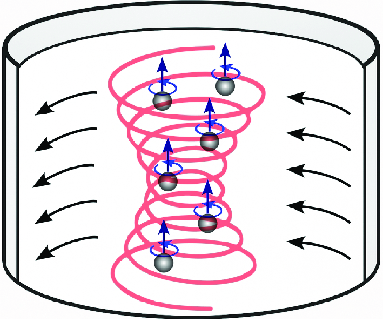

1. Introduction
The control of acoustic waves within confined geometries has led to remarkable advancements across various scientific and technological domains. Cylindrical resonator cavities, characterised by their closed, rigid walls and fluid-filled interiors, serve as fundamental platforms for exploring intricate acoustic phenomena. Kundt (Reference Kundt1866) was the first to describe the use of acoustic standing waves to gather initially uniformly distributed particles at specific planes of acoustic pressure, either nodal or antinodal. More recently, a renewed interest in studying wave dynamics within cylindrical resonators has grown significantly due to their potential to manipulate microparticles and cells within acoustofluidic microcavities (Coakley Reference Coakley1997; Spengler et al. Reference Spengler, Jekel, Christensen, Adrian, Hawkes and Coakley2000; Goddard & Kaduchak Reference Goddard and Kaduchak2005; Lenshof et al. Reference Lenshof, Evander, Laurell and Nilsson2012; Wang et al. Reference Wang, Castro, Hoyos and Mallouk2012; Gralinski et al. Reference Gralinski, Raymond, Alan and Neild2014; Gutiérrez-Ramos et al. Reference Gutiérrez-Ramos, Hoyos and Ruiz-Suárez2018; Pavlic & Dual Reference Pavlic and Dual2021; Santos et al. Reference Santos2021; Rocha et al. Reference Rocha, Silva, Sales, D’Amato, Leite and Silva2023; Fuchsluger et al. Reference Fuchsluger, Pastina, Ecker, Mitteramskogler, Voglhuber-Brunnmaier, Andrianov, Cselyuszka and Jakoby2024). In turn, acoustofluidics uses the forces of ultrasonic waves to manipulate and control cells or micro/nanoparticles within microfluidic structures.
One of the earliest theoretical explorations into cylindrical resonators can be credited to Rayleigh (Reference Rayleigh1945, pp. 49–68). This seminal work later became a fundamental part of textbooks, as seen in Morse (Reference Morse1948, pp. 381–431). These studies extensively employed the classical wave equation, formulated in terms of acoustic pressure only, and its time-harmonic equivalent, the Helmholtz equation. However, these existing models have overlooked the impact of losses within the viscous boundary layer adjacent to the cylindrical cavity walls. The wave dynamics, incorporating viscous boundary layer effects under the isentropic hypothesis (where entropy remains constant with heat transfer being negligible), encompasses two distinct spatial scales: the acoustic wavelength (
 $\lambda$
) and the viscous boundary layer thickness (
 $\delta$
), where
 $\lambda \gg \delta$
. Some recent efforts have been dedicated to deriving boundary conditions for acoustic pressure in cavities with curved boundaries, where the radius of curvature is much larger than the thickness of the viscous boundary layer, primarily motivated by numerical simulation purposes (Bach & Bruus Reference Bach and Bruus2018; Berggren, Bernland & Noreland Reference Berggren, Bernland and Noreland2018).
We focus our investigation on cylindrical cavity resonators similar to those used in acoustofluidic applications for manipulating cells and microparticles. This manipulation is driven by ultrasonic forces and torques, namely, the acoustic radiation force (Doinikov Reference Doinikov2003; Baudoin & Thomas Reference Baudoin and Thomas2019) and torque (Zhang & Marston Reference Zhang and Marston2011a
,Reference Zhang and Marston
b
; Silva, Lobo & Mitri Reference Silva, Lobo and Mitri2012; Gong, Marston & Li Reference Gong, Marston and Li2019), and Stokes’ drag by acoustic streaming (Rednikov & Sadhal Reference Rednikov and Sadhal2011; Baasch, Pavlic & Dual Reference Baasch, Pavlic and Dual2019). The acoustic radiation force can concentrate suspended particles at either pressure nodes or antinodes of a standing wave, depending on their density and compressibility relative to the surrounding fluid (Gor’kov Reference Gor’kov1962). Additionally, negative radiation forces, such as those arising from acoustic Bessel beams, have also been investigated (Zhang & Marston Reference Zhang and Marston2011c
). The acoustic radiation torque may induce rotation around the particle principal axis due to spin angular momentum transfer from the wave to the particle, which is referred to as the spin-torque effect (Silva Reference Silva2014; Toftul et al. Reference Toftul, Bliokh, Petrov and Nori2019; Lopes et al. Reference Lopes, Lima, Leão Neto and Silva2020). Drag forces can be caused by acoustic streaming, represented by sustained flow rolls. However, polystyrene particles with a diameter larger than
 ${1.4}\, {{\mu} \textrm{m}}$
in water, under the action of a
 ${2}\, {\mathrm{MHz}}$
ultrasonic wave, are more responsive to the acoustic radiation force (Barnkob et al. Reference Barnkob, Augustsson, Laurell and Bruus2012). In this study, the critical diameter is expected to be of the same order of magnitude as reported by Barnkob et al. (Reference Barnkob, Augustsson, Laurell and Bruus2012), which considers similar cavity dimensions and operational frequencies. Both studies assume no-slip boundary conditions at the walls and account for viscous effects as the primary dissipation mechanism. However, differences in cavity geometry may influence the balance between acoustic radiation and streaming forces, potentially leading to a difference in the critical particle diameter in cylindrical systems.
Given the focus on micro-sized particles and cells above this critical diameter, our analysis is solely devoted to scenarios involving acoustic radiation force and spin angular momentum.
To investigate the mentioned acoustofluidic phenomena in rigid cylindrical cavities, we employ a perturbation method in the fluid conservation equations with the adiabatic assumption to obtain the Helmholtz equation for the linear acoustic pressure. The boundary conditions at the walls deviate from the conventional Neumann condition, typically used to describe lossless wave phenomena, by a perturbation of the order of the viscous boundary layer thickness divided by the wavelength,
 $\delta /\lambda$
. The resultant boundary-value problem for the acoustic pressure is solved for a vortex excitation applied at the cavity’s base, giving rise to either a single- or dual-frequency mode (the occurrence of two single modes simultaneously) configuration in the resonator. While the single modes depend only on frequency selection, the dual modes are also related to the cavity’s aspect ratio.
The developed theory is showcased for an acoustofluidic microcavity resonator excited by sinusoidal vibration at the bottom. We found that near resonance, the amplitude of the nonlinear effects for decoupled axial and vortex modes scales with the square of the shear wave number (Tijdeman Reference Tijdeman1975),
 $\textit{Sh}^2=(R/\delta )^2$
, where
 $R$
is the cavity radius. Moreover, the findings show that single-vortex modes produce spin angular momentum only in the axial direction, whereas dual modes create an additional transverse spin component as a result of the nonlinear interaction between axial and transverse ultrasonic waves, even without vortex excitation. Finally, the obtained results are compared with those computed with the finite element method using the linear thermoviscous model with rigid and adiabatic walls. Excellent agreement is found between the computational simulations and proposed theory. To conclude, by incorporating effects of the viscous boundary layer and offering a detailed examination of the nonlinear acoustic phenomena within cylindrical resonators, our work extends the existing lossless theory (Barmatz & Collas Reference Barmatz and Collas1985; Xu et al. Reference Xu, Cai, Chen, Li, Wang, Meng, Xu, Wang, Wu and Zheng2019; Leão-Neto et al. Reference Leão-Neto, Hoyos, Aider and Silva2021) and provides a robust basis for future numerical and experimental studies.
2. Physical model
2.1. Fluid dynamics equations
Consider a cylindrical microcavity resonator of radius
 $R$
and height
 $H$
filled with a quiescent viscous liquid. The rigid boundary walls that enclose the cavity are represented by
 $\mathcal{S}=S_{{T}}\cup S_{{B}}\cup S_{{L}}$
, with
 $S_{{T}}$
,
 $S_{{B}}$
and
 $S_{{L}}$
denoting the top, bottom and lateral boundary, respectively. The Eulerian reference frame is placed in the centre of
 $S_{{B}}$
at rest. The fluid flow is described by a mass density
 $\rho$
, pressure
 $p$
and fluid velocity
 $\tilde {\boldsymbol{v}}$
as a function of position
 $\boldsymbol{r}$
and time
 $t$
. To take advantage of the cavity’s shape, cylindrical coordinates are adopted
 $(\varrho , \varphi ,z)$
, with position vector
 $\boldsymbol{r} = \varrho \, \boldsymbol{e}_\varrho + \varphi \, \boldsymbol{e}_\varphi + z\, \boldsymbol{e}_z$
, in which
 $\boldsymbol{e}_i$
 $(i=\varrho ,\varphi ,z)$
represents the transverse radial, azimuthal and axial unit vectors. The origin of the coordinate system is set at the centre of the bottom of the cavity.
The unperturbed state of the liquid is described by an ambient density
 $\rho _0$
, pressure
 $p_0$
, adiabatic speed of sound
 $c_0$
, isentropic compressibility
 $\kappa _0=1/\rho _0 c_0^2$
, and dynamic
 $\eta _0$
and bulk
 $\zeta _0$
viscosity. These parameters remain constant for the analysis under consideration. The physical parameters of water are listed in table 1.
Physical properties of water at
 ${25}\,{^{\circ }\mathrm{C}}$
(Holmes, Parker & Povey Reference Holmes, Parker and Povey2011).

In the investigation of acoustic wave propagation within the enclosed cavity, the process is assumed to be isentropic, with both internal heat generation and conduction effects being considered negligible. This assumption allows for a simplification in complex interactions between thermodynamic and acoustic phenomena. A detailed analysis of adopting the isentropic hypothesis is presented in Appendix A.
The fluid dynamics equations are described by the mass and linear momentum conservation equations along with the density-pressure constitutive relation,
 \begin{align} \partial _t \rho + \boldsymbol{\nabla } \cdot (\rho {\boldsymbol{v}}) &= 0, \end{align}
 \begin{align} \partial _t (\rho {\boldsymbol{v}}) -\boldsymbol{\nabla } \cdot \left (\boldsymbol{\sigma } - \rho {\boldsymbol{v}}{\boldsymbol{v}} \right ) &= \boldsymbol{0}, \end{align}
 \begin{align} p &= c_0^2 \rho . \end{align}
The stress tensor is given by
 \begin{equation} \boldsymbol{\sigma } = \left [- p + \left ( \zeta _0 -\dfrac {2}{3}\eta _0 \right ) (\boldsymbol{\nabla } \cdot {\boldsymbol{v}})\right ] \unicode{x1D644} + \eta _0\! \left [\boldsymbol{\nabla } {\boldsymbol{v}} + \left (\boldsymbol{\nabla } {\boldsymbol{v}}\right )^{\text{T}} \right ], \end{equation}
where
 $\unicode{x1D644}$
is the unit tensor and the superscript
 $^{\text{T}}$
denotes the transpose of a tensor. The energy conservation equation is not needed to describe acoustic phenomenon within the isentropic hypothesis.
2.2. Perturbation expansion
An acoustic wave can be injected into the microcavity through a time-harmonic oscillation with angular frequency
 $\omega$
, at the bottom surface
 $S_{{B}}$
at
 $z=0$
. By considering that
 $S_{{B}}$
moves back and forth along the
 $z$
axis, we express the surface displacement as
 \begin{equation} S(\varrho , \varphi ; t) = d(\varrho , \varphi )\, \textrm {e}^{-\textrm {i} \omega t + \textrm {i} \frac {\pi }{2}}, \quad \varrho \lt R, \end{equation}
where
 $d$
is the displacement function. The phase
 $\pi /2$
is added here for convenience. Note that no lateral motion of
 $S_{{B}}$
will be taken into account in our analysis. The corresponding excitation velocity is
 \begin{equation} v_{{ex}}(\varrho ,\varphi ; t) =\partial _t{S} = \omega \, d(\varrho ,\varphi )\, \textrm {e}^{-\textrm {i} \omega t}. \end{equation}
In the present analysis, the peak velocity of
 $S_{{B}}$
is assumed to be much smaller than the speed of sound in the medium. In terms of the Mach number, this implies
 $\textit{Ma}= \omega d_0/c_0\ll 1$
, in which
 $d_0$
is the given peak displacement at
 $S_{{B}}$
. To solve the fluid dynamics equations given in (2.1) in this approximation, the fields are conveniently expanded as
 \begin{align} \rho (\boldsymbol{r},t) &= \rho _0[1 + \textit{Ma} \,\tilde {\rho }_1(\boldsymbol{r}) \textrm {e}^{-\textrm {i} \omega t}], \end{align}
 \begin{align} p(\boldsymbol{r},t) &= p_0 + \textit{Ma} \kappa _0^{-1}\, \tilde {p}_1(\boldsymbol{r}) \textrm {e}^{-\textrm {i} \omega t}, \end{align}
 \begin{align} {\boldsymbol{v}}(\boldsymbol{r},t) &= \boldsymbol{0} + \textit{Ma} c_0 \,\tilde {\boldsymbol{v}}_1(\boldsymbol{r}) \textrm {e}^{-\textrm {i} \omega t}. \end{align}
The dimensionless amplitude functions
 $\tilde {p}_1$
,
 $\tilde {\rho }_1$
and
 $\tilde {\boldsymbol{v}}_1$
represent respectively the pressure, density and fluid velocity in the linear approximation. Hereafter, a variable with a tilde accent is a dimensionless quantity. It is convenient to express the excitation in terms of a dimensionless function
 $\tilde {v}_{{b}}$
,
 \begin{equation} v_{{ex}} = \textit{Ma} c_0 \tilde {v}_{{b}}\,\textrm {e}^{-\textrm {i} \omega t},\quad \text{with} \ \tilde {v}_{{b}} = \frac {d(\varrho ,\varphi )}{d_0} . \end{equation}
In acoustofluidic cavities based on piezoelectric ceramics, the peak displacement at the bottom is generally
 $d_0\approx {1}\, {\mathrm{nm}}$
in the low-megahertz range (Tran-Huu-Hue et al. Reference Tran-Huu-Hue, Levassort, Felix, Damjanovic, Wolny and Lethiecq2000). Hence, the expected Mach number for a water-filled cavity at
 ${1}\, {\mathrm{MHz}}$
is
 $\textit{Ma}\sim 10^{-6}$
.
2.3. Linear acoustics equations
A viscous fluid supports both compressional and shear flows. So we introduce a decomposition of the fluid velocity as a compressional part (
 $\tilde {\boldsymbol{v}}^{\textit{c}}$
) plus a shear part (
 $\tilde {\boldsymbol{v}}^{\textit{s}}$
),
 \begin{equation} \tilde {\boldsymbol{v}}_1 = \tilde {\boldsymbol{v}}_{{c}} + \tilde {\boldsymbol{v}}_{{s}}. \end{equation}
The compressional component is irrotational, while the shear part is incompressible,
 \begin{equation} \boldsymbol{\nabla } \times \tilde {\boldsymbol{v}}_{{c}} = \boldsymbol{0} \quad \text{and}\quad \boldsymbol{\nabla } \cdot \tilde {\boldsymbol{v}}_{{s}} =0. \end{equation}
Replacing (2.5a
), (2.5c
) and (2.7) into (2.1a
), while expressing the dimensionless mass density with (2.1c
) as
 $\tilde {\rho }_1=\tilde {p}_1$
, we obtain the first-order dimensionless pressure as
 \begin{equation} \tilde {p}_1 = - \frac {\textrm {i} c_0}{\omega } \boldsymbol{\nabla } \cdot \tilde {\boldsymbol{v}}_{{c}}. \end{equation}
Inserting (2.5c
) with (2.7) into (2.1b
) and using (2.9) followed by the vector operator identity
 $\boldsymbol{\nabla }(\boldsymbol{\nabla }\cdot \square ) = \nabla ^2\square + \boldsymbol{\nabla }\times \boldsymbol{\nabla }\times \square$
, we arrive at the compressional and shear velocities, respectively
 \begin{align} \tilde {\boldsymbol{v}}_{{c}} &= - \frac {\textrm {i} c_0 }{\omega } \left (1- \textrm {i} \Gamma _{{c}}\right ) \boldsymbol{\nabla } \tilde {p}_1, \end{align}
 \begin{align} \tilde {\boldsymbol{v}}_{{s}} &= \frac {\textrm {i} \eta _0 }{\omega \rho _0}\nabla ^2 \tilde {\boldsymbol{v}}_{{s}}. \end{align}
The compressional damping factor (in the fluid bulk) is given by
 \begin{equation} \Gamma _{{c}} =\kappa _0 \omega \left (\zeta _0 + \frac {4}{3}\eta _0 \right ). \end{equation}
Taking the divergence of (2.10a ) and using (2.9) yields the Helmhotz equation for pressure:
 \begin{align} \big (\nabla ^2 + k_{{c}}^2\big) \tilde {p}_1 = 0, \quad \text{with} \ k_{{c}} = \left ( 1 + \frac {\textrm {i}}{2}\Gamma _{{c}}\right )k. \end{align}
The real part of the compressional wavenumber is
 $k=\omega /c_0$
, with the associated acoustic wavelength being
 $\lambda = 2\pi /k$
. Equation (2.10b
) can be recast in the form
 \begin{align} \big(\nabla ^2 + k_{{s}}^2\big) \tilde {\boldsymbol{v}}_{{s}} = \boldsymbol{0},\quad k_{{s}} =\frac {1+\textrm {i}}{\delta }, \end{align}
where
 \begin{equation} \delta =\sqrt {\frac {2 \eta _0}{\rho _0 \omega }} \end{equation}
is the thickness of the viscous boundary layer. According to table 1, this thickness is
 $\delta ={0.53}\, {{\mu} \textrm{m}}$
for water at room temperature (
 ${25}\,{^{\circ }\mathrm{C}}$
) and
 ${1}\, {\mathrm{MHz}}$
.
3. Compressional normal modes
3.1. Eigenfunctions of the Helmholtz equation
The regular eigenfunctions, i.e. independent solutions to (2.12) in cylindrical coordinates, for a rigid cavity resonator can be expressed by (Morse Reference Morse1948, p. 398)
 \begin{equation} \tilde {p}_1 = J_n (k_\varrho \varrho ) \big[a_1\cos \!\left (k_z z\right ) + a_2 \sin (k_z z)\big] \big(b_1\textrm {e}^{\textrm {i} n \varphi } + b_2 \textrm {e}^{-\textrm {i} n \varphi }\big), \end{equation}
where
 $J_n$
represents the
 $n$
th-order Bessel function with
 $n\in \mathbb{Z}$
. The coefficients
 $a_i$
and
 $b_i$
(
 $i=1,2$
) will be determined from the boundary conditions (4.2). Furthermore, from (2.12), we find that the axial (
 $k_z$
) and circular (
 $k_\varrho$
) wavenumbers are related by
 \begin{equation} k_z^2 + k_\varrho ^2 = (1+\textrm {i} \Gamma _{{c}})\, k^2. \end{equation}
Roots of equation
 $\textrm {d} J_n(x)/\textrm {d} x =0$
for
 $n,m\leqslant 4$
.

3.2. Natural frequency modes
Prior to commencing the analysis of a viscous fluid-filled cavity resonator, it is beneficial to present the natural frequency of the system. For a rigid cavity with boundary surface denoted by
 $S$
, the pressure satisfies the Neumann boundary condition at the walls,
 \begin{equation} \boldsymbol{n}\cdot \boldsymbol{\nabla } \tilde {p}_1{\kern-3pt}\left |_{\boldsymbol{r}\in S } = 0,\right . \end{equation}
where
 $\boldsymbol{n}$
is the normal unit vector of the surface
 $S$
pointing outwardly. In this case, the axial and circular wavenumbers become
 \begin{equation} k_{z}^l = \frac {l \pi }{H}, \quad k_{\varrho }^{nm} = \frac {j_{nm}'}{R}, \end{equation}
with
 $n,m,l=0, 1, 2, \ldots$
The function
 $j_{nm}'$
represents a root of equation
 $\textrm {d} J_n(x)/\textrm {d} x =0$
. Note that
 $k_\varrho ^{nm}$
is the eigenvalue of both natural modes with a positive or negative
 $n$
. Table 2 shows the roots considering mode numbers in the interval
 $0\leqslant n,m\leqslant 5$
. According to (3.2), the compression wavenumber followed by the angular frequency of the natural mode
 $(n\,m\,l)$
are given by
 \begin{align} k^{nml}_0 &= \sqrt {\left (k_{z}^l\right )^2 + \big(k_{\varrho }^{nm}\big)^2}, \end{align}
 \begin{align} \omega ^{nml}_0 &= c_0 k^{nml}_0. \end{align}
Purely radial waves of mode
 $(0\,m\,0)$
appear along the radial vector
 $\boldsymbol{e}_\varrho$
. Likewise, waves aligned with the
 $z$
axis are present in mode
 $(0\,0\,l)$
. Waves corresponding to displacement along the azimuthal direction, represented by
 $\boldsymbol{e}_\varphi$
, manifest in mode
 $(n\,0\,0)$
. Finally, modes characterised by
 $(n\,m\,0)$
are designated as circular modes.
3.3. Scaling parameter
Viscous effects near solid boundaries are significant due to the steep velocity gradients imposed by the no-slip condition. For acoustofluidic experimental settings in the megahertz range and above, the following condition involving the viscous boundary layer thickness is assumed to hold:
 \begin{equation} \delta \ll R, H, \lambda . \end{equation}
We define the scaling parameter for the viscous-boundary thickness as
 \begin{equation} \epsilon \equiv \frac { 2\pi \delta }{\lambda } = k \delta \ll 1. \end{equation}
Note that this parameter scales with frequency as
 $\epsilon \sim \sqrt {\omega }$
. At a frequency of
 ${1}\,{\mathrm{MHz}}$
, the scaling parameter for water is
 $\epsilon =0.0022$
, whereas at
 ${1}\,{\mathrm{GHz}}$
, it increases to
 $\epsilon =0.069$
. It is further assume that the peak displacement at the bottom is much smaller than the thickness of the viscous boundary layer,
 $d_0\ll \delta$
.
The compressional damping factor
 $\Gamma _{{c}}$
can also be expressed in terms of
 $\epsilon$
by using (2.11),
 \begin{equation} \Gamma _{{c}} = \left (\frac {2}{3} + \frac {\zeta _0}{2\eta _0}\right )\epsilon ^2. \end{equation}
Again, for water at the same conditions, we have
 $\Gamma _{{c}} = {5.06 \times 10^{-6}}$
. Equation (3.8) reveals that damping in the cavity bulk is generally very small.
4. No-slip boundary conditions
The core of establishing pressure boundary conditions lies in enforcing the no-slip condition on the cavity walls, expressed as
 \begin{equation} \tilde {\boldsymbol{v}}_{{c}}(\boldsymbol{r}) + \tilde {\boldsymbol{v}}_{{s}}(\boldsymbol{r}) = \begin{cases} \tilde {v}_{{b}}\boldsymbol{e}_z, \quad & \boldsymbol{r}\in S_{{b}},\\ \boldsymbol{0}, \quad & \boldsymbol{r}\in S_{{t}} \cup S_{{w}}. \end{cases} \end{equation}
Here, the ultrasonic actuation with velocity
 $\tilde{v}_{{b}}$
is exclusively applied at the bottom of the resonator cavity. In Appendix B, we derive the boundary conditions for the linear pressure based on (4.1). The pressure should adhere to the following conditions:
 \begin{align} \left [\partial _z + \epsilon\! \left . \frac {1+\textrm {i}}{2k}\big(\partial _{z}^2 + k^2\big)\right ] \tilde {p}_1\right |_{z=0}\; =\;& \textrm {i} k {\tilde v}_b, \end{align}
 \begin{align} \left [\partial _z - \epsilon\! \left . \frac {1+\textrm {i}}{2k}\big(\partial _{z}^2 + k^2\big )\right ] \tilde {p}_1\right |_{z=H} \;=\;& 0, \end{align}
 \begin{align} \left \{ \partial _\varrho - \epsilon\! \left . \frac {1+\textrm {i}}{2k} \left [\frac {1}{\varrho }\partial _\varrho (\varrho \partial _\varrho ) + k^2\right ] \right \}\tilde {p}_1\right |_{\varrho =R} \;=\;& 0. \end{align}
The boundary conditions stated in (4.2) can be interpreted as an impedance boundary condition, specifically incorporating a second-order derivative of pressure. This result is in agreement with that obtained by Bach & Bruus (Reference Bach and Bruus2018, (25)) for cavities with arbitrary curved geometry.
Figure 1 presents a schematic representation summarising the boundary value problem for the pressure field within a cylindrical acoustic cavity. A time-harmonic excitation is applied at the cavity’s base.
Sketch of the acoustic cavity with rigid walls. The yellow area represents the viscous boundary layer, with a thickness
 $\delta$
. The pressure
 $\tilde {p}_1$
obeys the Helmholtz equation, shown in light blue. The fluid velocity behaviour within the boundary layer is represented at the top
 $z=H$
and wall
 $\varrho =R$
. The red arrows denote the shear velocity
 $\tilde {\boldsymbol{v}}_s$
, while the blue and green arrows represent the tangential components of the compressional velocity
 $\tilde {\boldsymbol{v}}_{{c}} - \tilde {v}_{{c},z}\boldsymbol{e}_z$
and
 $\tilde {\boldsymbol{v}}_{{c}} - \tilde {v}_{{c},\varrho }\boldsymbol{e}_\varrho$
. The axial velocity excitation
 $\tilde {v}_{{b}}\boldsymbol{e}_z$
is denoted by black arrows at the bottom. The coordinate system is set at the centre of the cavity’s bottom.

5. Resonance states
The presence of viscous boundary layers near the cavity walls modifies the resonance frequency (
 $\omega ^{nml}$
) from its natural (lossless) value. This frequency shift has been analysed in rectangular acoustics (Bach & Bruus Reference Bach and Bruus2018). To quantify this effect, we conveniently introduce a correction under the assumption of small damping, expressed as
 \begin{equation} \omega ^{nml} = \left (1 - \frac {1}{2}\Gamma ^{nml}_\delta \right ) \omega _0^{nml}, \end{equation}
where
 $\omega _0^{nml}$
represents the natural resonance frequency in the absence of dissipation and
 $\Gamma ^{nml}_\delta$
is the boundary-layer damping factor. The approximation
 $\Gamma _\delta ^{nml} \ll 1$
holds for fluids with low to moderate viscosity, such as water and vegetable oils, where boundary-layer losses remain small compared with the overall resonance behaviour. The explicit derivation of
 $\Gamma _\delta ^{nml}$
is provided in Appendix D, following the boundary condition formulation.
The associated wavenumber at resonance is
 $k^{nml} = \omega ^{nml}/c_0$
. As the system operates near a resonance state
 $(n\,m\,l)$
, the axial and circular wavenumber are expected to slightly deviate from those of the natural modes:
 \begin{align} k_\varrho ^{nml} &= k_{\varrho }^{nm} + \Delta {k}_{\varrho }^{nml}, \quad \big |\Delta {k}_{\varrho }^{nml} R \big |\ll 1, \end{align}
 \begin{align} k_z^{nml} &= k_{z}^l + \Delta {k}_{z}^{nml}, \quad \big |\Delta {k}_z^{nml} H \big |\ll 1. \end{align}
The deviation term in (5.2a
) will be determined from the boundary condition (4.2c
). The obtained result is then used in (3.2) to derive the axial deviation
 $\Delta k_z^{nml}$
.
In Appendix C, we derive
 $\Delta k_\varrho ^{nml}$
by solving the boundary condition (4.2c
). Accordingly, we have
 \begin{equation} \Delta {k}_{\varrho }^{nml} = \begin{cases} \pm \textrm {i} \sqrt {\left (1 + \textrm {i}\right )\dfrac {\epsilon ^{00l}}{k_0^{00l} R}} k_0^{00l},\quad &n,m=0,\\[9pt] (1+\textrm {i})\dfrac {\epsilon ^{nml} }{2k_0^{nml}R} \dfrac {n^2 + \big(k_{z}^l R\big)^2 }{n^2-\big(k_{\varrho }^{nm} R\big)^2} k_{\varrho }^{nm}, \quad &\text{otherwise}. \end{cases} \end{equation}
Here, we have introduced the damping parameter
 $\epsilon ^{nml}$
evaluated at the natural frequency
 $\omega _0^{nml}$
:
 \begin{align}&\, \epsilon ^{nml} = k_0^{nml}\delta ^{nml}, \end{align}
 \begin{align}& \delta ^{nml}= \sqrt {\frac {2 \eta _0}{\rho _0 \omega _0^{nml}}}. \end{align}
We now proceed to obtain the axial wavenumber at resonance. Using (3.2), we find
 \begin{equation} \big [k_z^{nml}(k)\big ]^2 = \big (1+\textrm {i} \Gamma _{{c}}^{nml}\big )k^2 - \big (k_\varrho ^{nml}\big )^2, \end{equation}
where the compressional damping factor at the natural frequency values
 $\Gamma _{{c}}^{nml} |_{\epsilon =\epsilon ^{nml}}$
. We replace (5.2a
) into (5.5), use
 $k=\omega /c_0$
and expand the result around the resonance frequency
 $\omega =\omega ^{nml}$
, while keeping the result to its lowest-order,
 \begin{align} \nonumber \big [k_z^{nml}(\omega )\big ]^2&= \big (k_{z}^l\big )^2 + \frac {2 k_0^{nml}}{c_0}\big(\omega -\omega ^{nml}\big) + \big(\textrm {i} \Gamma _{{c}}^{nml} -\Gamma _\delta ^{nml}\big) \big (k_0^{nml}\big )^2 - 2 k_{\varrho }^{nm} \Delta k_\varrho ^{nml}\\ &\quad -\delta _{n,0}\delta _{m,0} \big (\Delta k_\varrho ^{00l}\big )^2, \end{align}
where
 $\delta _{ij}$
is the Kronecker delta function. Note that
 $(\Delta k_\varrho ^{00l})^2$
varies linearly with
 $\epsilon _{nml}$
. If the axial mode is suppressed (
 $l=0$
), we have
 \begin{align} \big [k_z^{nm0}(\omega )\big ]^2 = \frac {2 k_0^{nm0}}{c_0}\big(\omega -\omega ^{nm0}\big) + \big (\textrm {i} \Gamma _{{c}}^{nm0}-\Gamma _\delta ^{nm0}\big )\big(k_0^{nm0}\big)^2 - 2 k_{\varrho }^{nm}\Delta k_\varrho ^{nm0}. \end{align}
6. Single-mode configuration
6.1. Vortex excitation
In accordance with (2.4), the velocity excitation required to generate a mode with positive vorticity in the cavity is described as
 \begin{equation} \tilde {v}_{{b}} = J_{n}\big(k_{\varrho }^{nm}\varrho \big) \textrm {e}^{ \textrm {i} n \varphi }. \end{equation}
The induced pressure amplitude rotates counterclockwise when observed from above the
 $x{-}y$
plane – see figure 1. In this case, the azimuthal coefficients in (3.1) become
 $b_1=1$
and
 $b_2=0$
. Conversely, when the angular factor is
 $\textrm {e}^{-\textrm {i} n\varphi }$
, the induced pressure rotates clockwise from the same viewpoint, and
 $b_1=0$
and
 $b_2=1$
. For the case where
 $n=0$
, the excitation produces a non-vortex mode within the resonator, with
 $b_1=b_2=1/2$
.
6.2. Pressure coefficients
Substituting (3.1) and (6.1) into (4.2a
) and (4.2b
), we arrive at a system of linear equations for the pressure coefficients
 $a_1$
and
 $a_2$
:
 \begin{align} \boldsymbol{A} \left ( \begin{matrix} a_1 \\ a_2 \end{matrix} \right ) &= \left ( \begin{matrix} \textrm {i} (k H)^2 \\ 0 \end{matrix} \right ), \end{align}
 \begin{align} \boldsymbol{A} &= \left ( \begin{matrix} \epsilon \chi & k_z k H^2 \\[4pt] k_z k H^2 \sin (k_z H) + \epsilon \chi \cos (k_z H)& - k k_z H^2 \cos (k_z H)+ \epsilon \chi \sin ( k_z H) \end{matrix} \right ), \end{align}
with
 $\chi = (1+\textrm {i}) (k^2-k_z^2 ) H^2/2$
. Terms of order
 $\epsilon \Gamma _{{c}}$
were discarded. Also, we have taken the approximation
 $J_n(k_\varrho ^{nml} \varrho )\approx J_n(k_{\varrho }^{nm} \varrho )$
. According to Cramer’s rule, the solution of (6.2) is given by
 \begin{align} a_1 &= \frac {\textrm {i} k}{k_z} \frac { k k_z H^2 \cos (k_z H) - \epsilon \chi \sin (k_z H)} { k k_z H^2 \sin (k_z H) + 2 \epsilon \chi \cos (k_z H)},\\[-11pt] \nonumber \end{align}
 \begin{align} a_2 &= \frac {\textrm {i} k}{k_z} \frac {k k_z H^2 \sin (k_z H) + \epsilon \chi \cos (k_z H)} {k k_z H^2 \sin (k_z H) + 2 \epsilon \chi \cos (k_z H)}. \end{align}
It is important to compare the magnitude of the pressure coefficients. Referring to (5.2b
), we observe that
 $\cos (k_z z) \approx \cos (k_z^l z)$
and
 $\sin (k_z z) \approx \sin (k_z^l z)$
. This implies that
 $a_2/a_1 \sim \epsilon$
, allowing us to safely neglect the term
 $a_2 \sin (k_z z)$
in (3.1). Therefore, the pressure near the resonance is assumed to be
 \begin{equation} \tilde {p}_1^{nml}(\boldsymbol{r}) = a_1 J_n\big(k_\varrho ^{nm} \varrho \big) \cos \big (k_z^l z\big) \textrm {e}^{\textrm {i} n \varphi }. \end{equation}
The amplitude coefficient
 $a_1$
and the boundary-layer factor
 $\Gamma _\delta ^{nml}$
are determined in Appendix D. Gathering the result, we have
 \begin{align} a_1 &= \frac {\textrm {i} (2-\delta _{l,0})}{k_0^{nml}H} \frac {\dfrac {1}{2}\omega ^{nml}}{\omega - \omega ^{n m l} + \dfrac {1}{2} \textrm {i}\,\omega ^{nml} \Gamma ^{n m l} }, \end{align}
 \begin{align} \Gamma ^{nml} &= \Gamma _\delta ^{nml} + \Gamma _{{c}}^{nml}, \end{align}
 \begin{align} \Gamma _\delta ^{nml} &= \epsilon ^{nml} \left \{ \left [\frac {2-\delta _{l,0}}{k_0^{nml} H} + \frac {1}{k_0^{nml} R} \frac {\big(k_{z}^l R\big)^2 + n^2 }{\big(k_{\varrho }^{nm} R\big)^2-n^2} \right ] \left (\frac {k_{\varrho }^{nm}}{k_0^{nml}}\right )^2 + \frac { \delta _{n,0} \delta _{m,0}}{ k_0^{nml} R} \left (\frac {k_{z}^{l}}{k_0^{nml}}\right )^2 \right \}. \end{align}
The total damping factor
 $\Gamma ^{nml}$
is determined by using the wavenumbers related to the natural frequency
 $\omega _0^{nml}$
.
6.3. Pressure field
We now replace (6.5a
) into (6.4) to obtain the pressure amplitude of the single-vortex mode
 $(n\,m\,l)$
,
 \begin{align} {p}_1^{nml} &= {A}^{nml} R^{nml} \Psi ^{nml},\quad (n,m,l=0, 1, 2, \ldots ), \end{align}
 \begin{align} {A}^{nml} &= \frac {2-\delta _{l,0}}{\Gamma ^{nml} k_0^{nml}H}, \end{align}
 \begin{align} {R}^{nml} &=\frac {1}{2}\frac { \omega ^{nml}\Gamma ^{nml} } { \omega - \omega ^{nml}\left (1 + \frac {1}{2}\textrm {i} \, \Gamma ^{nml}\right )}, \end{align}
 \begin{align} \Psi ^{nml} &= J_n\big (k_\varrho ^{nm} \varrho \big) \cos \big(k_z^l z\big) \textrm {e}^{\textrm {i} \left (n \varphi +\frac {\pi }{2}\right )}. \end{align}
where
 ${A}^{nml}$
is the pressure amplitude,
 ${R}^{nml}$
is the resonance function and
 $\Psi ^{nml}$
is the cavity’s wavefunction. The pressure amplitude scales inversely with the total damping factor
 $(\Gamma ^{nml})^{-1}$
and the height-to-wavelength ratio
 $(k_0^{nml} H)$
. At the resonance frequency, we have
 $ R^{nml}|_{\omega =\omega ^{nml}} = -\textrm {i}$
. Hence, the pressure becomes
 \begin{equation} p_1^{nml}|_{\omega =\omega ^{nml}}= -\textrm {i} {A}^{nml} \Psi ^{nml}. \end{equation}
We note also that the pressure phase is composed of three components, namely, the resonance
 $(\varphi _{{r}}^{nml})$
, spatial (
 $\varphi _{{s}} ^{nml}$
) and vortex
 $(n\varphi )$
phase:
 \begin{equation} \varphi ^{nml} = \varphi _{{r}}^{nml} + \varphi _{{s}}^{nml}+ n\varphi + \frac {\pi }{2}. \end{equation}
6.4. Fluid velocity fields
We can determine the fluid velocity in the fluid bulk by using (2.10a ),
 \begin{equation} \tilde {\boldsymbol{v}}_{{c}}^{nml} = -\textrm {i} {A}^{nml} {R}^{nml}\, \tilde {\boldsymbol{\nabla }}\Psi ^{nml}, \end{equation}
where
 $\tilde {\boldsymbol{\nabla }}=(k_0^{nml})^{-1}\boldsymbol{\nabla }$
is the scaled gradient to the natural wavenumber. Simultaneously, the shear velocity near the boundaries can be calculated by applying (6.9) in combination with (B1) and (B7),
 \begin{equation} \tilde {\boldsymbol{v}}_{{s}}^{nml} = -\textrm {i} {A}^{nml} {R}^{nml} \Big[ \Big ( \textrm {e}^{\textrm {i} k_{{s}} z} + (-1)^l \textrm {e}^{\textrm {i} k_{{s}} (H-z)} \Big) \tilde {\boldsymbol{\nabla }}_{\!\boldsymbol{e}_z} + \textrm {e}^{\textrm {i} k_{{s}} (R-\varrho )} \tilde {\boldsymbol{\nabla }}_{\!\boldsymbol{e}_\varrho } \Big]\Psi ^{nml}, \end{equation}
with
 $\tilde {\boldsymbol{\nabla }}_{\!\boldsymbol{n}}= (\unicode{x1D644} - \boldsymbol{n}\boldsymbol{n} )\cdot \tilde {\boldsymbol{\nabla }}$
being the scaled surface gradient. The shear velocity is confined in the viscous boundary as it decays exponentially away from the cavity walls.
7. Dual-mode configuration
Thus far, our focus has been on single-mode resonances. Nevertheless, it is possible to use multimode excitation inside the cavity. Multimode excitation refers to the simultaneous activation of two or more modes with the same eigenfrequency. Consider the natural frequency
 $\omega _0^{nml}$
associated with the single mode
 $(n\,m\,l)$
, which is excited through the applied vibration at the resonator’s bottom, as described by (6.1). This natural frequency can also be linked to two other modes,
 $(n_1\,m_1\,l_1)$
and
 $(-n_1\,m_1\,l_1)$
, through the relation
 $\omega _0^{nml} = \omega _0^{n_1 ml}$
. The superposition of these modes represents a dual-mode configuration, denoted by
 $ ( n\,m\,l ) + ( n_1\,m_1\,l_1 )$
. Since
 $\omega _0^{n_1 ml} = \omega _0^{(-n_1) ml}$
, the formation of triple modes is also possible, which is the superposition of
 $ ( n\,m\,l )$
,
 $ ( n_1\,m_1\,l_1 )$
, and
 $ ( -n_1\,m_1\,l_1 )$
. For clarity, the analysis proceeds with the dual-mode configuration. Although triple modes may introduce intriguing possibilities, their analysis is left to future work.
When the single-mode natural frequencies are equal, we have the wavenumber relation
 \begin{equation} k_0^{nml} = k_0^{n_1m_1l_1}. \end{equation}
Using (3.4), we find that this configuration can only occur when the cavity’s aspect ratio satisfies the condition
 \begin{equation} \frac {R}{H} = \frac {1}{\pi }\sqrt {\frac {\big(j_{n_1 m_1}^{\prime}\big)^2 - \big(j_{n m}^{\prime}\big)^2}{l^2 - l_1^2}}. \end{equation}
Using this relation, we can induce the dual-mode configuration in a cavity by changing the excitation velocity in (6.1) to
 \begin{equation} \tilde {v}_{{b}} = J_{n}\big(k_{\varrho }^{nm}\varrho \big) \textrm {e}^{ \textrm {i} n \varphi } + J_{n_1}\big (k_{\varrho }^{n_1m_1}\varrho \big) \textrm {e}^{ \textrm {i} n_1 \varphi }. \end{equation}
Note that the velocity excitation applied at the base of the cavity is a single-frequency excitation
 $\omega$
, as highlighted in (2.6). The pressure inside the cavity is given by
 \begin{equation} \tilde {p}_1=\tilde {p}_{n ml}^{n_1 m_1l_1} =\tilde {p}_1^{n ml} + \tilde {p}_1^{n_1 m_1l_1}. \end{equation}
From (6.6a ), we can express (7.4) by
 \begin{equation} \tilde {p}_{n ml}^{ n_1 m_1 l_1} = A^{n m l} R^{n m l} \Psi ^{n m l} + {A}^{n_1m_1 l_1}R^{n_1 m_1 l_1} \Psi ^{ n_1 m_1l_1}. \end{equation}
8. Nonlinear acoustic phenomena
We present important phenomena governed by acoustic fields of the magnitude
 $\textrm {O}(\textit{Ma}^2)$
, which include considerations of energy density, radiation force and spin angular momentum. These effects are described by time-averaged quantities derived from the product of first-order pressure and velocity fields. It can be demonstrated that the time average of the product of two linear complex-amplitude fields
 $f(\boldsymbol{r})\,\textrm{e}^{-\textrm {i} \omega t}$
and
 $g(\boldsymbol{r})\,\textrm{e}^{-\textrm {i} \omega t}$
is given by
 \begin{align} \overline {f(\boldsymbol{r})\,\textrm {e}^{-\textrm {i} \omega t} g(\boldsymbol{r})\,\textrm {e}^{-\textrm {i} \omega t}} = \frac {\omega }{2\pi } \int _{-\frac {\pi }{\omega }}^{\frac {\pi }{\omega }} {\mathrm{Re}}\big[f(\boldsymbol{r})\,\textrm {e}^{-\textrm {i} \omega t}\big] {\mathrm{Re}}\big[g(\boldsymbol{r})\,\textrm {e}^{-\textrm {i} \omega t}\big] \,\textrm {d} t = \frac {1}{2} {\mathrm{Re}}\!\left [f(\boldsymbol{r}) g^*(\boldsymbol{r})\right ], \nonumber\\[-6pt]\end{align}
where the asterisk
 $^*$
denotes complex conjugation. To facilitate the upcoming analysis, the second-order fields will be expressed in terms of the pressure amplitude squared
 $|\tilde {p}_1|^2$
. Moreover, given the disparity in dimensions between the viscous boundary layer thickness and the microcavity size, the predominant velocity component of second-order acoustic fields analysed here arises from the compressional fluid velocity.
8.1. Acoustic energy density
The time-averaged acoustic energy density, often referred to as the energy landscape, offers a spatial representation of energy distribution within the cavity. This provides valuable insights into the system’s behaviour and performance. The energy landscape (
 $E$
) arises from the contributions of both kinetic (
 $E_{{k}}$
) and potential (
 $E_{{p}}$
) acoustic energy densities,
 \begin{align} {E} &= {E}_{{k}} +{E}_{{p}}, \end{align}
 \begin{align} {E}_{{k}}&= E_0\left |\tilde {\boldsymbol{v}}_{{c}}\right |^2, \end{align}
 \begin{align} {E}_{{p}}&=E_0 \left |\tilde {p}_1\right |^2, \end{align}
where
 $E_0 = \textit{Ma}^2 \rho _0 c_0^2/4$
is the characteristic energy density of the cavity. Using (2.10a
) allows us to express the kinetic energy density as
 \begin{equation} {E}_{{k}}= \frac {E_0}{k^2} \boldsymbol{\nabla }\! \tilde {p}_1 \cdot \boldsymbol{\nabla }\! \tilde {p}_1^*= \frac {E_0}{k^2}\left (\frac {1}{2}\nabla ^2|\tilde {p}_1|^2-{\mathrm{Re}}\big[\tilde {p}_1^*\nabla ^2 \tilde {p}_1\big]\right )= E_0\left (\frac {1}{2k^2}\nabla ^2 + 1\right ) |\tilde {p}_1|^2. \end{equation}
Here, we have used (2.12). Hence, the energy density reads
 \begin{align} {E} = {E}_{{k}} + {E}_{{p}} = 2 E_0 \left (\frac {1}{4k^2}\nabla ^2 + 1\right ) |\tilde {p}_1|^2. \end{align}
We define the dimensionless energy density as
 $\tilde {E}=E/E_0$
. Using (6.6a
) and (7.5), we obtain the single-mode energy density as
 \begin{equation} \tilde {E}^{nml} = 2\big|A^{nml}R^{nml} \big |^2 \left (\frac {1}{4}\tilde {\nabla }^2 + 1\right ) \big|\Psi ^{nml}\big|^2, \end{equation}
where
 $\tilde {\nabla }^2=k^{-2}\nabla ^2$
is the scaled Laplacian. Inserting (7.5) into (8.4), we obtain the energy density of the dual mode as
 \begin{equation} \tilde {E}^{n_1 m_1l_1}_{nml} = \tilde {E}^{nml} + \tilde {E}^{ n_1 m_1l_1} + \tilde {E}_{{cross}}. \end{equation}
The cross term of the energy density is given by
 \begin{equation} \tilde {E}_{{cross}}= 4 A^{nml} A^{n_1m_1 l_1} {\mathrm{Re}} \left[ \big (R^{nml}\big)^* R^{n_1m_1 l_1} \left (\frac {1}{4}\tilde {\nabla }^2 + 1\right ) \big({\Psi ^{nml}}\big)^* \Psi ^{n_1 m_1l_1}\right ]. \end{equation}
While the single-mode energy density does not depend on the azimuthal angle
 $\varphi$
, the crossed energy does.
8.2. Dissipated power
The time-averaged dissipated power
 $P^{nml}$
for a specific mode
 $(n\,m\,l)$
is linked with the energy stored in the cavity
 $(E_{{stored}})$
through the concept of the cavity’s quality factor, or
 $Q$
factor. As discussed by Hahn et al. (Reference Hahn, Leibacher, Baasch and Dual2015), this relationship is expressed as
 \begin{equation} Q = \frac {\omega ^{nml}}{P^{nml}} \int _{V_0} E^{nml} \, \textrm {d} V = \frac {\omega ^{n m l}}{\Delta \omega ^{n m l}}. \end{equation}
Here, the stored energy is derived from the integration of the energy density over the cavity volume
 $V_0$
. The term
 $\Delta \omega ^{n ml}$
represents the
 ${-3}\,{\rm dB}$
bandwidth of the resonance line, which is determined by solving the equation
 $|R^{n m l}(\omega )|^2 = ({1}/{2})$
, subsequently leading to
 $\Delta \omega ^{n m l} = \omega ^{n m l} \Gamma ^{n m l}.$
Replacing the bandwidth into (8.8) gives the
 $Q$
factor as
 \begin{equation} Q =\frac {1}{\Gamma ^{nml}}. \end{equation}
Consequently, the dissipated power by the cavity is
 \begin{equation} P^{nml}= \Gamma ^{nml}\omega ^{nml}\int _{V_0} E^{nml} \, \textrm {d} V. \end{equation}
8.3. Acoustic radiation force on a small particle
An important application of acoustofluidic microcavities is the contactless manipulations of small particles. We consider a spherical particle of volume
 $V_{{p}}$
, isentropic compressibility
 $\kappa _{{p}}$
and density
 $\rho _{{p}}$
. Moreover, the particle in consideration is assumed to be much smaller than the wavelength. In this case, the acoustic radiation force exerted on a particle at position
 $\boldsymbol{r}$
is given by (Gor’kov Reference Gor’kov1962)
 \begin{align} \boldsymbol{F}&= -V_{{p}}\boldsymbol{\nabla } U, \end{align}
 \begin{align} U &= f_\kappa {E}_{{p}} -\frac {3}{2}f_\rho {E}_{{k}}, \end{align}
 \begin{align} f_\kappa &= 1 - \frac {\kappa _{{p}}}{\kappa _0}, \quad f_\rho = 2 \frac {\rho _{{p}} - \rho _0}{2\rho _{{p}}+ \rho _0}, \end{align}
where
 $U$
is the Gor’kov potential density, and
 $f_\kappa$
and
 $f_\rho$
are respectively the compressional and density contrast factors. After inserting the kinetic (8.2b
) and potential (8.2c
) energy densities into (8.11b
), we find the dimensionless Gor’kov potential density
 $(\tilde {U}=U/E_0)$
as
 \begin{equation} \tilde {U} = \left [ f_\kappa - \frac {3}{2} f_\rho \left ( \frac {1 }{2 } \tilde {\nabla }^2 +1 \right )\right ] \left |\tilde {p}_1\right |^2. \end{equation}
Substituting (6.6a ) into this equation yields the single-mode Gor’kov potential
 \begin{equation} \tilde {U}^{nml} = \big |A^{nml} R^{nml} \big|^2 \left [ f_\kappa - \frac {3}{2} f_\rho \left (\frac {1 }{2 } \tilde {\nabla }^2+1 \right )\right ] \big|\Psi ^{nml}\big|^2. \end{equation}
The Gor’kov potential of a dual mode is obtained by replacing (7.4) into (8.12),
 \begin{equation} \tilde {U}^{n_1 m_1l_1}_{nml} = \tilde {U}^{nml} + \tilde {U}^{ n_1 m_1 l_1} + \tilde {U}_{{cross}}. \end{equation}
The cross term of the dual-mode potential is
 \begin{align} \tilde {U}_{{cross}} = 2 A^{nml} A^{n_1m_1 l_1} {\mathrm{Re}} \! \left \{\big (R^{nml}\big )^* R^{n_1m_1 l_1} \left [ f_\kappa - \frac {3}{2} f_\rho \left ( \frac {1 }{2 } \tilde {\nabla }^2 +1 \right )\right ] {\Psi ^{nml}}^* \Psi ^{n_1 m_1l_1}\right \}. \end{align}
8.4. Spin angular momentum
The spin angular momentum density of an acoustic wave can be expressed by (Bliokh & Nori Reference Bliokh and Nori2019; Lopes et al. Reference Lopes, Lima, Leão Neto and Silva2020)
 \begin{equation} \boldsymbol{S} = \frac {\rho _0}{2 \omega }{\mathrm{Im}}\!\left [{\boldsymbol{v}}_{{c}}^* \times {\boldsymbol{v}}_{{c}}\right ], \end{equation}
which is given in the SI units of
 $\mathrm{J\,s\,m^{-3}}$
. Substituting (2.10a
) into (8.16) allows us to express the acoustic spin as
 \begin{align} \boldsymbol{{S}} &=\frac {1}{2\rho _0\omega ^3}{\mathrm{Im}} \!\left [ \boldsymbol{\nabla }\! {p}_1^* \times \boldsymbol{\nabla }\! {p}_1\right ]= \frac {1}{2\rho _0\omega ^3}{\mathrm{Im}} \!\left [\boldsymbol{\nabla } \times \left ({p}_1^*\boldsymbol{\nabla } \!{p}_1\right ) \right ]= \frac {1}{\omega ^2}\boldsymbol{\nabla } \times \dfrac {1}{2}\mathrm{Re}\! \left [ {p}_1^* {\boldsymbol{v}}_c\right ]\nonumber\\&= \frac {1}{\omega ^2}\boldsymbol{\nabla } \times \boldsymbol{I}. \end{align}
It is important to note that the spin angular momentum is a measure of the circulation of acoustic intensity, defined as
 $\boldsymbol{I} = ({1}/{2}) \text{Re} [ {p}_1^* \boldsymbol{v}_c ]$
. The acoustic spin density forms a solenoidal field, meaning
 $\nabla \cdot \boldsymbol{S} = 0$
.
We define the dimensionless acoustic spin density as
 $\tilde {\boldsymbol{S}}= \omega \boldsymbol{S}/E_0$
. To obtain the spin of a single-vortex mode at the resonance,
 $\omega =\omega ^{nml}$
, we substitute (6.6a
) into (8.17),
 \begin{equation} \tilde {\boldsymbol{S}}^{nml} = 2 \big|{A}^{nml}R^{nml} \big |^2{\mathrm{Im}}\! \left [ \tilde {\boldsymbol{\nabla }} \times \big( {\Psi ^{nml} }^* \tilde {\boldsymbol{\nabla }}\Psi ^{nml} \big) \right ]. \end{equation}
For the dual-mode configuration, one has
 \begin{align} \tilde {\boldsymbol{S}}_{nml}^{n_1m_1l_1} = \tilde {\boldsymbol{S}}^{nml} + \tilde {\boldsymbol{S}}^{ n_1 m_1l_1} + \tilde {\boldsymbol{S}}_{{cross}}, \end{align}
with the spin cross term being
 \begin{align} \nonumber \tilde {\boldsymbol{S}}_{{cross}} &= 2 A^{nml} A^{n_1m_1l_1} {\mathrm{Im}}\big \{ \tilde {\boldsymbol{\nabla }} \times \big [ \big (R^{nml}\big )^* R^{n_1m_1 l_1} \big (\Psi ^{nml} \big )^* \tilde {\boldsymbol{\nabla }}\Psi ^{n_1m_1l_1}\big . \big .\\ &\quad \big . \big .+ \big (R^{n_1m_1l_1}\big )^* R^{nm l}\big (\Psi ^{n_1 m_1l_1}\big )^* \tilde {\boldsymbol{\nabla }}{\Psi ^{nml} } \big ]\big \}. \end{align}
8.5. Acoustic spin and radiation torque connection
When a particle is immersed in an acoustic field, it may experience a radiation torque resulting from the transfer of angular momentum from the field to the particle. In the long-wavelength scattering regime, the acoustic radiation torque
 $\boldsymbol{\tau }$
exerted on an absorptive spherical particle (by a vortex beam or vortex standing wave) is connected to the spin density
 $\boldsymbol{S}$
through the relation (Silva Reference Silva2014, (29))
 \begin{align} \boldsymbol{\tau } &= \gamma \boldsymbol{S}, \end{align}
 \begin{align} \gamma &= -\frac {12 \pi c_0}{k^2} \big( {\mathrm{Re}}\!\left [s_1\right ]+ \left |s_1\right |^2{\kern-2pt} \big ), \end{align}
where
 $\gamma$
is the gyroacoustic factor and
 $s_1$
is the dipole scattering coefficient, which depends on energy dissipation by the particle. The derivation of (8.21a
) is based on the angular momentum flux formalism (Maidanik Reference Maidanik1958).
Using (8.21a
), we recover the expression for the axial radiation torque exerted by a Bessel vortex beam on a spherical particle of radius
 $ a$
, located at position
 $ \boldsymbol{r}$
, as previously derived by Zhang (Reference Zhang2018) and on-axis by Zhang & Marston (Reference Zhang and Marston2011
b). In the notation of Zhang (Reference Zhang2018), the dipole scattering coefficient is given by
 $ s_1 = 1 + \textrm {i} (ka)^3 (f_{2\textit{r}} + \textrm {i} f_{2\textit{i}})/6,$
where
 $ f_{2\textit{r}} = f_\kappa$
– as defined in (8.11c
) – and
 $ f_{2\textit{i}} = (3 \delta _{\textit{p}}/2a) f_\kappa ^2$
, with
 $ \delta _{\mathrm{p}}$
denoting the thickness of the viscous boundary layer surrounding the particle. This leads to the expression
 $ \gamma = 2\pi a^3 \omega f_{2\textit{i}}$
. The axial spin density
 $ S_z$
of an
 $ n$
th-order Bessel vortex beam is given by Lopes et al. (Reference Lopes, Lima, Leão Neto and Silva2020) as
 $S_z = 2 n (I_0/c_0) \sin \beta \, J_n(k \varrho \sin \beta ) J_n'(k \varrho \sin \beta ) / \omega k \varrho$
, where
 $ I_0 = p_0^2/2\rho _0 c_0$
is the time-averaged beam intensity,
 $ p_0$
is the pressure amplitude,
 $ \beta$
is the conical angle of the beam’s wave vector, and the prime symbol denotes differentiation with respect to the function’s argument. Substituting
 $ \gamma$
and
 $ S_z$
into (8.21a
), we obtain the axial radiation torque,
 \begin{equation} \tau _z = 6\pi n f_\kappa ^2 \delta _{{p}} a^2 \frac {I_0}{c_0} \sin ^2\beta \, J_n'(k \varrho \sin \beta ) \frac {J_n(k \varrho \sin \beta )}{k \varrho \sin \beta }. \end{equation}
This expression exactly matches the axial radiation torque derived by Zhang (Reference Zhang2018, (14a)) and Zhang & Marston (Reference Zhang and Marston2011b , (10)). We thus confirm the general validity of the spin-torque relation (8.21a ), which applies to spherical particles undergoing power absorption due to either internal dissipation or viscous losses in the surrounding fluid.
It is also important to mention that the radiation torque exerted by an acoustic wave (acoustic beam or standing wave) on a spherical particle of arbitrary size has also been derived using the angular momentum flux formalism (Zhang & Marston Reference Zhang and Marston2011 b; Silva et al. Reference Silva, Lobo and Mitri2012; Zhang & Marston Reference Zhang and Marston2014). These works demonstrate that torque arises from energy dissipation during scattering, which can occur either within the particle itself or in the surrounding viscous boundary layer. In the on-axis case, the proportionality of torque on power absorption for spheres in standing waves or beams (Zhang & Marston Reference Zhang and Marston2011 b, (10)) is not limited to the case of absorption associated with the dipole response emphasised in (8.22).
Recently, Bliokh & Nori (Reference Bliokh and Nori2019) formulated the concept of acoustic spin density within the framework of canonical field theory, drawing parallels with its electromagnetic analogue. Building on this formalism, Toftul et al. (Reference Toftul, Bliokh, Petrov and Nori2019) derived the spin-torque relationship given in (8.21a ) for isotropic particles. Subsequently, Lima et al. (Reference Lima, Leão-Neto, Marques, Silva, Lopes and Silva2020)and Lopes et al. (Reference Lopes, Lima, Leão Neto and Silva2020) extended the spin-torque relation to encompass small axisymmetric particles, such as spheroids, thereby broadening its applicability to more complex geometries.
9. Acoustofluidic cylindrical resonators
The use of acoustofluidic cylindrical resonators stands as a pivotal technique in processes such as cell/particle focusing (Goddard & Kaduchak Reference Goddard and Kaduchak2005) and precise patterning (Rocha et al. Reference Rocha, Silva, Sales, D’Amato, Leite and Silva2023). Cylindrical resonators excited at the bottom serve to adeptly form particle aggregates within a defined levitation plane. The number of levitation planes is determined by the axial mode number
 $l$
.
9.1. Acoustic single modes
Two modes of particular interest are the axial and the transverse modes. The energy landscape of these modes near the resonance frequency
 $(\omega \approx \omega ^{nml})$
are derived by substituting (6.6) into (8.5). The result yields respectively
 \begin{align} \tilde {E}^{l} &= \big |A^l R^{l} \big|^2, \end{align}
 \begin{align} \tilde {E}^{nm} &= \left |A^{nm} R^{nm} \right |^2 \left [J_n\!\left (\tilde {\varrho }^{nm} \right )\left [\frac {J_n^{\prime}\!\left (\tilde {\varrho }^{nm}\right )}{\tilde {\varrho }^{nm}} + J_n^{\prime\prime}\!\left (\tilde {\varrho }^{nm}\right )\right ] +\left [J_n'\!\left (\tilde {\varrho }^{nm}\right )\right ]^2 + 2 J_n^2\!\left (\tilde {\varrho }^{nm}\right ) \right ], \end{align}
where
 $A^l=A^{00l}$
,
 $A^{nm}=A^{nm0}$
,
 $R^{l}=R^{00l}$
and
 $R^{nm}=R^{nm0}$
, and
 $\tilde {\varrho }^{nm}=k_\varrho ^{nm}\varrho$
. Note that the energy density of the vortex mode exhibits circular symmetry, while it remains spatially constant for the axial mode.
Now, we turn our analysis to the Gor’kov potential near the resonance frequency. For the axial mode
 $(0\,0\,l)$
, this potential is obtained from (8.13). Accordingly, we have
 \begin{equation} \tilde {U}^{l} = \tfrac {1}{2} \big |A^l R^l\big |^2 \big [\big (2f_\kappa + 3f_\rho \big ) \cos ^2 \! \tilde {z}^l - 3f_\rho \big ], \end{equation}
where
 $\tilde {z}^l=k_z^l z$
. The particles will be trapped at the Gor’kov potential minimum by the action of the acoustic radiation force. When
 $2f_\kappa + 3f_\rho \gt 0$
, the potential minima is in the axial pressure nodes at
 $z_{{min}}=(2\ell +1)H/2l$
, with
 $\ell =0,1,\ldots ,l-1$
. If
 $2f_\kappa + 3f_\rho \lt 0$
, the minima is at the pressure antinodes in
 $z_{{min}} = \ell H/l$
, where
 $\ell =0,1,\ldots ,l$
. The axial radiation force per unit length is obtained by taking the negative gradient of (9.2):
 \begin{equation} {F}_z^l =\frac {E_0 V_{{p}}}{2} \big |A^l R^l\big |^2 \big (2f_\kappa + 3f_\rho \big ) \sin \!\big ( 2\tilde {z}^l \big ). \end{equation}
Considering the transverse mode
 $(n\,m\,0)$
, we find from (8.13) that the Gor’kov potential is
 \begin{align} \nonumber \tilde {U}^{nm} &= \frac {1}{2} \left |A^{nm} R^{nm} \right |^2 \left \{ \left (2f_\kappa - 3f_\rho \right ) \left [J_n\!\left (\tilde {\varrho }^{nm}\right )\right ]^2 \vphantom{\frac {J_n'\!\left (\tilde {\varrho }^{nm}\right )}{\tilde {\varrho }^{nm}}} \right .\\ &\quad\left . - 3 f_\rho \left [J_n'\!\left (\tilde {\varrho }^{nm}\right )\right ]^2 - 3 f_\rho J_n\!\left (\tilde {\varrho }^{nm} \right ) \left [ J_n^{\prime\prime}\!\left (\tilde {\varrho }^{nm} \right ) + \frac {J_n'\!\left (\tilde {\varrho }^{nm}\right )}{\tilde {\varrho }^{nm}} \right ]\right \}. \end{align}
The Gor’kov potential here has no azimuthal dependence on
 $\varphi$
. For the sake of brevity, we will analyse the radial trapping around the symmetry axis of the cavity only. To do so, we use the asymptotic form of the Bessel function for small arguments,
 $J_n(x) \approx 2^{-n} x^n ( 1/n! - 1/4[(n+1)!])$
, with
 $x \rightarrow 0$
. The radial radiation force of the non-vortex and first vortex mode (
 $n=0,1$
) are given by
 \begin{align} {F}_\varrho ^{0m} &= f_\kappa E_0 V_{{p}}\big |A^{0m} R^{0m} \big |^2 k_\varrho ^{0m} \varrho + \textrm {O}\big (\varrho ^3\big ), \end{align}
 \begin{align} {F}^{1m}_\varrho &= -\big ( 2f_\kappa + 3f_\rho \big ) E_0 V_{{p}} \big |A^{1m} R^{1m} \big |^2 \varrho + \textrm {O}\big (\varrho ^3\big ). \end{align}
Some conclusions can be drawn from the analysis here. Particles in the non-vortex mode
 $(0\,m)$
can either be repelled from
 $(f_\kappa \gt 0)$
or attracted to
 $(f_\kappa \lt 0)$
the cavity axis. In the first-vortex mode
 $(1\,m)$
, particles will be trapped at the cavity axis if
 $2f_\kappa + 3f_\rho \gt 0$
. Conversely, they will be repelled if
 $2f_\kappa + 3f_\rho \lt 0$
.
We proceed with the derivation of the spin angular momentum for modes with
 $|n|\gt 0$
. Substituting (6.6d
) into (8.18), we find the only non-zero spin component is the axial one, which is given by
 \begin{align} \tilde {S}_z^{nm} = 2n \big|A^{nm}R^{nm} \big|^2 \frac { \big[J_n^2\!\big (k_\varrho ^{nm} \varrho \big )\big]^{\prime}}{k_\varrho ^{nm}\varrho }. \end{align}
Modes with no vorticity (
 $n=0$
) lack spin. Note that the acoustic radiation torque exerted on a small spherical particle by a Bessel vortex wave beam or standing wave) derived by Zhang (Reference Zhang2018, (12)) is proportional to the axial spin given in (9.6). Moreover, a detailed examination of (9.6), using the expression
 $\lim _{x \rightarrow 0} [{J_n^2(x)} ]'/x = {\delta _{n,\pm 1}}/{2}$
, indicates that only the
 $(\pm 1\,m)$
mode exhibits spin along the
 $z$
axis. Hence,
 \begin{equation} \lim _{\varrho \rightarrow 0}\tilde {S}_z^{\pm 1m} = \pm \big |A^{1m}R^{1m} \big|^2. \end{equation}
The amplitudes of the energy density and Gor’kov potential as well as the spin density can be obtained using (5.4b ), (6.5b ) and (6.6b ). It can be shown that
 \begin{equation} \big|A^l\big|^2, \big|A^{nm}\big|^2 \sim \textit{Sh}^2= \left (R/\delta \right )^2. \end{equation}
The parameter
 $\textit{Sh}=R/\delta$
is known as the shear wave number of the cavity (Tijdeman Reference Tijdeman1975). This suggests that for decoupled axial and vortex resonant modes, increasing the shear wave number (
 $\textit{Sh}$
) reduces the relative influence of boundary-layer-induced viscous dissipation on the bulk resonance response.
9.2. Acoustic dual modes
One potential application of dual modes in cylindrical cavities is to levitate cells or microparticles, providing an additional degree of freedom: rotation around an axis of symmetry. The dual mode, composed of an axial mode
 $(0\,0\,l)$
, ensures the formation of
 $l$
levitation planes at the mid-height of the cavity, while circular modes
 $(n\,m\,0)$
are responsible for clustering particles and inducing a spin-torque on the trapped particles. From (7.2), we note that the cavity’s aspect ratio to host the dual mode
 $ (0\,0\,l) + ( n\, m\, 0)$
is
 \begin{equation} \frac {R}{H} = \frac {j^{\prime}_{nm}}{l \pi }. \end{equation}
Moreover, according to (8.14) and (8.19), the Gor’kov potential and spin density of this mode near the resonance
 $(\omega \approx \omega ^{l}\approx \omega ^{nm0})$
can be expressed by
 \begin{align}& \tilde {U}_{l}^{nm} = \tilde {U}^{l} + \tilde {U}^{nm}+ \tilde {U}_{{cross}}, \end{align}
 \begin{align}&\quad \tilde {\boldsymbol{S}}_{l}^{nm} = \tilde {{S}}^{nm}_z \boldsymbol{e}_z + \tilde {\boldsymbol{S}}_{{cross}}. \end{align}
The cross terms are calculated with (8.15) and (8.20). Accordingly, we have
 \begin{align} \nonumber \tilde {U}_{{cross}}&= A^lA^{nm}\big|R^{l}R^{nm}\big | J_{n_1}\big(\tilde {\varrho }^{nm}\big) \bigg [\big(2f_\kappa - 3 f_\rho \big) \cos \!\left (n\varphi - \Delta \varphi _l^{nm}\right )\vphantom{\frac {k_z^l}{k}} \\ &\quad + \;3f_\rho \bigg(\frac {k_z^l}{k}\bigg)^2\cos \!\left (n\varphi + \Delta \varphi _l^{nm}\right ) \bigg ]\cos \tilde {z}^l, \end{align}
 \begin{align} \nonumber \tilde {\boldsymbol{S}}_{{cross}} &= 4 A^l A^{nm} \big|R^{l}R^{nm} \big| \bigg[ n \cos \big(n \varphi +\Delta \varphi _l^{nm}\big) \frac {J_{n}\big(\tilde {\varrho }^{nm}\big)}{\tilde {\varrho }^{nm}} \boldsymbol{e}_\varrho \\ & \quad -\sin\!\big(n \varphi +\Delta \varphi _l^{nm}\big) \, J_{n}'\big(\tilde {\varrho }^{nm}\big) \,\boldsymbol{e}_\varphi \bigg]\sin ^2 \tilde {z}^l, \end{align}
where the additional phase is
 $\Delta \varphi _l^{nm}=\angle (R^l)^*R^{n m}$
.
The spin component in (9.11b
) arises from the nonlinear interaction between two orthogonal modes,
 $(0\,0\,l)$
and
 $(n\,m\,0)$
. This component can be transferred to a suspended particle much smaller than the wavelength, resulting in an acoustic radiation torque on the particle (Zhang & Marston Reference Zhang and Marston2014). Consequently, the particle may rotate around one of its principal axes. Notably, even when
 $n=0$
, a spin component is still present, which is given by
 \begin{align} \tilde {\boldsymbol{S}}_{{cross}} &= 4 A^l A^{0m}\big|R^{l}R^{0m}\big| \sin \!\big(\Delta \varphi _l^{0m}\big) \, J_{1}\big(\tilde {\varrho }^{0m}\big) \sin ^2 \tilde {z}^l \,\boldsymbol{e}_\varphi . \end{align}
This result demonstrates that, even in the absence of vortex excitation, the spin angular momentum can still be generated in acoustofluidic resonators. It is also worth noting that metallic nanorods have been observed to rotate in acoustofluidic cylindrical cavities with a non-vortex excitation at the base (Wang et al. Reference Wang, Castro, Hoyos and Mallouk2012; Balk et al. Reference Balk, Mair, Mathai, Patrone, Wang, Ahmed, Mallouk, Liddle and Stavis2014). This rotational behaviour can be attributed to the spin-torque generated by the nonlinear interaction of orthogonal modes within the cavity.
Finally, we note that the cross terms also scale as
 $A^l A^{nm}\sim \textit{Sh}^2$
. We thus conclude that the amplitude of the Gor’kov potential and spin density of a dual mode also scales with shear wave number squared.
10. Theoretical versus numerical results
The theoretical results are now compared with finite element simulations conducted in Comsol Multiphysics 6.1 (Comsol AB, Sweden). Figure 2 illustrates the geometry set-up and mesh used in the simulations. Panel (a) depicts the lateral cross-sectional view of the model mesh, while panel (b) provides a cross-sectional view perpendicular to the cavity axis. The mesh in the fluid bulk (in blue) is characterised by a tetrahedral unstructured pattern with less dense elements. Near the walls, the viscous boundary layer (in yellow) is delineated by a finer structured mesh designed to capture the short-range variation of fluid flow. To compute the pressure and velocity field within the fluid inside the resonator, the Thermoviscous Acoustics, Frequency Domain Interface is employed. The simulations are executed using the physical parameters given in table 1 and under the adiabatic hypothesis, as discussed in Appendix A. The excitation velocity at the cavity bottom has a value of
 $|v_{{ex}}| ={1}\,{\textrm{mm}\, s^{-1}}$
. The radiation force is obtained for a polystyrene probe particle with acoustophoretic parameters
 $f_\kappa =0.3128$
and
 $f_\rho =0.0342$
. Finally, the simulations were conducted on a workstation featuring an Intel Xeon (R) E5–2690 processor with a
 ${3}\,{\mathrm{GHz}}$
clock, and equipped with
 ${384}\,{\mathrm{GB}}$
of memory. To compare the theoretical to numerical results, we use the coefficient of determination
 $\mathcal{R}^2$
, which measures how well a theoretical model explains the variability in a numerical data. A value of
 $\mathcal{R}^2=1$
indicates that the theoretical model perfectly matches the data, whereas
 $\mathcal{R}^2=0$
suggests that the theoretical model does no better than predicting the mean of the numerical data. The coefficient
 $\mathcal{R}^2$
is computed using the RSquared function in Mathematica software (ver. 10, Wolfram Inc, USA).
Visualisation of the finite element simulation mesh. (a) Lateral and (b) transverse cross-sectional view of the cavity. The mesh features the bulk region (blue) with a tetrahedral unstructured element and the viscous boundary layer (yellow) near the walls. The illustrated meshes are not to scale.

10.1. Single modes
In the results for single modes, a water-filled microcavity with dimensions
 $H=R={250}\, {{\mu} \textrm{m}}$
and a volume of
 $V_0={49}\, {\mathrm{nL}}$
is considered, representing a typical cavity in acoustofluidics devices (Rocha et al. Reference Rocha, Silva, Sales, D’Amato, Leite and Silva2023).
Here and in the subsequent figures, the
 $(n\, m\, l)$
notation is defined in (6.6). The
 $(0\,0\,1)$
and
 $(0\,1\,0)$
mode induced in a microcavity with
 $H=R={250}\, {{\mu} \textrm{m}}$
. (a,c) The pressure-frequency plot (magnitude and phase in blue and red line) using (6.6a
), and the corresponding resonance frequency and
 $Q$
factor. Blue and red dots indicate numerical results. (b) Gor’kov potential in the
 $x{-}z$
plane (background image) obtained from (9.2), with the related radiation force field (white arrows) acting on a
 ${10}\, {{\mu} \textrm{m}}$
-polystyrene probe particle. (d) The energy density computed with (9.1b) and (e) the Gor’kov potential for the probe particle calculate with (9.4). All fields are obtained at the corresponding resonance frequency. The vertical white lines delimit the theoretical (left) and numerical (right) results.

Figure 3 presents the
 $(0\,0\,1)$
and
 $(0\,1\,0)$
mode induced in the microcavity. The physical parameters of water used in this analysis are given in table 1, while panels (a) and (c) plot pressure versus frequency as given in (6.6a
), with
 $Q=796.10$
and
 $622.01$
, respectively. The resonance frequencies are
 ${2.9917}\, {\mathrm{MHz}}$
and
 ${3.6494}\, {\mathrm{MHz}}$
. Solid lines denote the theoretical result, while dots represent numerical data. Panel (b) depicts the Gor’kov potential density (background image) of the
 $(0\,0\,1)$
mode at the
 $xz$
plane, with white arrows illustrating the radiation force field. Probe particles will collect in the pressure node at the cavity’s midheight. Panels (d) and (e) show the energy density and Gor’kov potential of the
 $(0\,1\,0)$
mode. The related radiation force will trap particles in an annular region (in dark brown) in panel (e). The vertical white lines separate the theoretical (left) and numerical (right) results. The numerical data and the theoretical predictions show excellent agreement with
 $\mathcal{R}^2\sim 1$
. It is important to mention that in the numerical simulations, the degrees of freedom (DOFs) for the two-dimensional axisymmetric model used for the
 $(0\,0\,1)$
and
 $(0\,1\,0)$
modes is
 $288\,045$
. Larger numbers of DOF typically require more computational resources, both in terms of memory and processing power.
In figure 3(e), we note that the radiation force is zero in a ring with radius, denoted by
 $\varrho _{{r}}$
, which is a solution of the transcendent equation derived by inserting (9.4) into (8.11a
):
 \begin{equation} 3 f_\rho J_2\big(k_\varrho ^{01} \varrho _{{r}}\big )- (4 f_\kappa + 3 f_\rho ) J_0\big(k_\varrho ^{01} \varrho _{{r}}\big ) = 0. \end{equation}
The numerical solution to this equation yields
 $\varrho _{{r}} = 0.6117 R$
or
 $\varrho _{{r}}={152}\,{{\mu \textrm{m}}}$
, which is compatible with the particle trap region seen in panel (e).
Pure vortex mode
 $(1\,0\,0)$
and
 $(2\,0\,0)$
cases are considered here for the cavity described in figure 3. (a,e) Acoustic pressure plotted against frequency (magnitude and phase in blue and red line) using (6.6a
), along with the associated
 $Q$
factor and resonance frequency. The dots represent the numerical data. (b,f) Energy density calculated with (9.1b
). (c,g) Illustration of the Gor’kov potential for a
 ${10}\,{{\mu \textrm{m}}}$
polystyrene probe particle using (9.4). (d,h) Spin angular momentum according to (9.6). These fields are computed at the corresponding resonance frequency of each mode. The vertical white lines separate the theoretical (left) and numerical (right) results.

In figure 4, we illustrate the
 $(1\,0\,0)$
and
 $(2\,0\,0)$
mode within the same cavity introduced in figure 3. Panels (a) and (c) present the pressure plotted against frequency using (6.6a
). The associated
 $Q$
factor and resonance frequency are
 $436.97$
and
 ${1.7523}\,{\mathrm{MHz}}$
, and
 $453.37$
and
 ${2.9070}\,{\mathrm{MHz}}$
, respectively. The energy density given in (9.1b
) is shown in panels (b) and (f), while the Gor’kov potential from (9.4) for a
 ${10}\,{{\mu \textrm{m}}}$
polystyrene particle are seen in panels (c) and (g). The spin angular momentum, as given by (9.6), is shown in panels (d) and (h). These modes exhibit no levitation plane, indicating their purely vortex nature. Notably, the inward radiation force field is responsible for concentrating particles in the central portion of the resonator without levitation. The spatial pattern of the axial spin differs significantly between these modes. In the
 $(1\,0\,0)$
mode, collected particles experience a positive spin along the
 $z$
axis, peaking at
 $\varrho =0$
. Conversely, for the
 $(2\,0\,0)$
mode, the maximum axial spin, according to (9.6), occurs in a ring of radius
 $\varrho _{{s}}$
, which is determined by the solution of
 \begin{equation} \big [J_2^2\big(k_\varrho ^{20} \varrho _{{s}}\big )\big ]^{\prime\prime} =0 . \end{equation}
We find
 $\varrho _{{s}}={0.6759}R$
, yielding
 $\varrho _{{s}} = {169}\,{{\mu} \textrm{m}}$
. The axial spin potentially may induce a counterclockwise rotation on particles mostly depending on their geometric asymmetry. Note that the spin vanishes at
 $\varrho =0$
. In the numerical simulations, it was observed that the DOF of the three-dimensional model for the
 $(1\,0\,0)$
mode was
 $2\,705\,168$
. However, the DOF for the
 $(2\,0\,0)$
mode is
 $2\,475\,000$
. According to the coefficient of determination,
 $\mathcal{R}^2\sim 1$
, and visual inspection, the theoretical and numerical data show excellent agreement.
10.2. Dual modes
Here we consider the
 $(0\,1\,0)+(0\,0\,1)$
,
 $(1\,0\,0)+(0\,0\,1)$
and
 $(2\,0\,0)+(0\,0\,1)$
modes, as they correspond to the simplest modes for trapping and inducing torque on suspended particles. To develop these modes, the cavity’s aspect ratio should be respectively
 $R/H={1.2197}, {0.5860}$
,
 $0.9721$
. The height of all cavities is fixed to
 $H={250}\, {{\mu} \textrm{m}}$
. Also, the cavities are filled with water.
The
 $(0\,1\,0)+(0\,0\,1)$
mode for a cavity with aspect ratio
 $R/H={1.2197}$
. Panel (a) shows the magnitude (in blue) and phase (in red) of the acoustic pressure around the resonance frequency
 ${2.992}\, {\mathrm{MHz}}$
, plotted using (6.6a
). The numerical data are represented by dots. Panel (b) presents the Gor’kov potential density for the probe particle, with white arrows depicting the corresponding acoustic radiation force. The theoretical part of the potential is calculated using (9.10a
). Panel (c) exhibits the Gor’kov potential at the cavity mid-height, while panel (d) illustrates the magnitude of the transverse spin density, with white arrows denoting the related vector field. The theoretical part of the spin is computed with (9.10b
). The acoustic fields in panels (b), (c) and (d) are computed at the resonance frequency. The vertical white lines separate the theoretical (left) and numerical (right) results.

The
 $(1\,0\,0)+(0\,0\,1)$
mode for a cavity with
 $R/H={0.5860}$
and
 $R={250}\,{{\mu} \textrm{m}}$
. Panel (a) show the acoustic pressure (magnitude in blue and phase in red) around the resonance frequency
 ${2.991}\, {\mathrm{MHz}}$
, and plotted against frequency using (6.6a
). The dots represent the numerical data. Panel (b) presents the background map of the Gor’kov potential density for the probe particle. The theoretical part is computed using (9.10a
). Panel (c) exhibit the Gor’kov potential at the mid-height, while panels (d) and (e) illustrate the magnitude of the transverse and axial components of the spin density at the mid-height, respectively. The theoretical part of these components are calculated with (9.10b
). The white arrows in panel (d) correspond to the spin vector field. The acoustic fields are computed at the resonance frequency. The vertical white lines separate theoretical (left) and numerical (right) results.

The
 $(2\,0\,0)+(0\,0\,1)$
mode for a cavity with an aspect ratio of
 $R/H = {0.9721}$
and radius
 $ R = {250}\,{{\mu} \textrm{m}}$
. Panels (a) and (e) display the acoustic pressure around the resonance at
 ${2.992}\,{\mathrm{MHz}}$
, plotted as a function of frequency using (6.6a
), with numerical data shown as dots. Panel (b) depicts the Gor’kov potential density for a probe particle, calculated using (9.10a
). Panel (c) shows this potential at mid-height with the corresponding radiation force (white arrows), while panels (d) and (e) present the transverse and axial spin density magnitudes, calculated via (9.10b
). White arrows in panel (d) represent the spin vector field. The presented acoustic fields are computed at resonance, with vertical white lines dividing the theoretical (left) and numerical (right) results.

Figure 5(a) displays the acoustic pressure for the
 $(0\,1\,0)+(0\,0\,1)$
mode near the resonance frequency of
 ${2.992}\, {\mathrm{MHz}}$
, based on numerical simulations with 331 164 DOF. Panel (b) depicts the Gor’kov potential density in the
 $xz$
plane, along with the radiation force field shown by the white arrows. This potential is axisymmetric. Panel (c) shows the Gor’kov potential in the
 $x{-}y$
plane at the mid-height of the cavity, where the radiation force field (white arrows) traps particles in an annular region around the cavity central axis. Panel (d) presents the transverse spin component, with white arrows representing the related vector field. This spin arises due to the interaction between the transverse and axial velocity fields in the fluid. The spin exhibits characteristics of a solenoidal field (circulation). The theoretical and numerical results are in excellent agreement, with
 $\mathcal{R}^2 \sim 1$
, as seen by visual inspection.
Figure 6(a) shows the acoustic pressure for the
 $(1\,0\,0)+(0\,0\,1)$
mode around the resonance frequency of
 ${2.991}\,{\mathrm{MHz}}$
. A significant increase in the DOF (1 900 422) is noted, since this simulation requires a three-dimensional (3-D) mesh. Panel (b) presents the Gor’kov potential density in the
 $x{-}z$
plane, along with the radiation force field (white arrows). The potential in this plane is asymmetric due to the cross term in (9.11a
), which depends on the azimuthal angle
 $\varphi$
. In contrast, panel (c) shows a symmetric Gor’kov potential (with
 $U_{{cross}}=0)$
in the mid-height plane, where the radiation force field directs particles towards the cavity’s central axis. Panels (d) and (e) illustrate the transverse and axial spin components, respectively. The white arrows in panel (d) indicate the transverse spin field at mid-height, which results from the interaction between the transverse and axial fluid velocity fields. The axial spin component is most pronounced in the central region of the cavity, but diminishes near the lateral walls, while the transverse spin is predominantly oriented left-to-right and is approximately four times stronger than the axial spin. A circulating pattern is observed in the transverse spin field, consistent with the behaviour expected of a solenoidal field. We see that theoretical and numerical results show excellent agreement, with
 $\mathcal{R}^2 \sim 1$
, confirmed by visual inspection.
Figure 7(a) displays the acoustic pressure for the
 $(2\,0\,0)+(0\,0\,1)$
mode near the resonance frequency of
 ${2.992}\, {\mathrm{MHz}}$
, with 1 900 422 DOF in the numerical simulations. Panel (b) shows the Gor’kov potential density and radiation force field (white arrows) in the
 $x{-}z$
plane. Conversely, panel (c) illustrates the Gor’kov potential in the
 $x{-}y$
plane at mid-height, with the radiation force (white arrows) pointing towards the cavity’s axis of symmetry. The potential well is more shallow compared with the one in figure 6. Moreover, the simulation results exhibit some numerical fluctuations in the computed radiation force field. These fluctuations can, in principle, be mitigated by increasing the mesh resolution, though this would require greater computational memory. Panels (d) and (e) depict the transverse and axial spin components, respectively, with white arrows in panel (d) representing the transverse spin field at mid-height. The axial spin is more dominant in the annular region around the central axis. The transverse spin shows a circulating pattern around the dark spots at the edge of the cavity. Finally, theoretical and numerical results align closely, with
 $\mathcal{R}^2 \sim 1$
.
11. Discussion and conclusions
This study develops a detailed theoretical framework for understanding acoustic vortex modes in cylindrical resonator cavities, with particular attention to the role of viscous boundary layers. We employed the isentropic hypothesis to simplify the thermodynamic treatment by assuming negligible heat transfer within the fluid medium. This assumption is justified for acoustofluidic cavities with a low-amplitude excitation, where the induced temperature rise is expected to be much smaller than
 ${1}\,{\mathrm{K}}$
– see Appendix A.
Our investigation explored both single- and dual-mode configurations in microcavity resonators. The single modes analysed consisted of pure axial or pure transverse modes, while dual modes involved a simultaneous combination of axial and transverse modes. Dual modes are particularly noteworthy because they can exhibit spin angular momentum in both axial and transverse directions, offering new degrees of freedom for advanced manipulation of microparticles in acoustofluidic systems. Xu et al. (Reference Xu, Cai, Chen, Li, Wang, Meng, Xu, Wang, Wu and Zheng2019) experimentally observed the dual mode
 $(0\,2\,0)+(0\,0\,1)$
in a cavity made of silicon walls and glass plates, at
 ${4}\,{\mathrm{MHz}}$
. Notably, the cavity aspect ratio of
 $2.2526$
aligns with the theoretical prediction of (7.2).
Interestingly, even in the absence of vortex excitation, a transverse spin angular momentum can still be generated in acoustofluidic cylindrical resonators due to the nonlinear interaction between two orthogonal waves in the cavity. This result may provide an explanation for the observed rotation of metallic nanorods in acoustofluidic cavities (Wang et al. Reference Wang, Castro, Hoyos and Mallouk2012; Balk et al. Reference Balk, Mair, Mathai, Patrone, Wang, Ahmed, Mallouk, Liddle and Stavis2014), with a non-vortex excitation at the base.
We observed that nonlinear acoustic fields near resonance scale with the square of the shear wave number,
 $ \textit{Sh}^2 = (R/\delta )^2$
. Additionally, the theoretical results show excellent agreement with finite element simulations, as indicated by the coefficient of determination
 $ \mathcal{R}^2 \sim 1$
and visual inspection of the results. This consistency validates the accuracy of the theoretical approach and its potential for practical applications in describing acoustofluidic systems.
It is important to note that the rigid nature of the cavity ensures maximal efficiency by preventing energy leakage. In this case, the acoustic energy is dissipated primarily through viscous and thermal losses within the fluid rather than through boundary losses. In contrast, non-rigid cavities, such as those with elastic walls, allow energy to escape, reducing efficiency. The rigid cavity design, therefore, provides an optimal, though idealised, configuration. The hard-wall model for acoustofluidic cavity resonators establishes a theoretical benchmark for evaluating the performance limits of energy storage and particle manipulation efficiency in cavities constructed from practical materials such as glass and silicon.
The position of the acoustic excitation source can significantly influence the efficiency of the resonator. For example, side actuation has been shown to enhance the acoustic energy density in rectangular chambers compared with conventional bottom actuation (Qiu, Baasch & Laurell Reference Qiu, Baasch and Laurell2022). Baasch, Qiu & Laurell (Reference Baasch, Qiu and Laurell2024) later introduced a dimensionless acoustophoretic efficiency parameter and developed an in-flow focusing method to experimentally map the acoustic energy distribution across the entire channel. In addition to excitation position, the choice of piezoelectric material also affects energy transfer efficiency. Recent work demonstrated that lead-free transducers can achieve comparable or even superior performance to traditional lead zirconate titanate (PZT) transducers by facilitating efficient longitudinal mode coupling and suppressing transverse vibrational modes (Qiu Reference Qiu2024). Extending these strategies to cylindrical geometries may provide valuable pathways for improving chamber design and optimising transducer integration.
The numerical simulations of acoustic vortex modes in cylindrical resonators require a relatively high number of DOFs, typically in the low-million range. With this level of complexity, simulations demand significant computational resources, including increased memory capacity and processing power. Given the computational challenges, the development of accurate and efficient theoretical models is crucial for advancing the field of acoustofluidic resonators. Moreover, simplified computational models can also be employed, such as the one developed by Bach & Bruus (Reference Bach and Bruus2018), which uses effective boundary conditions that account for viscous boundary layer effects without requiring full resolution of these layers in numerical simulations. This computational approach can also be used as a validation tool for the present study.
Experimental verification of the predicted spin angular momentum in cavity resonators is important to validate the theoretical results presented in this study. Vortex acoustic waves can be excited in cylindrical resonators, constructed with materials such as silicon, glass and hard metals, by using a helicoidal transducer (Hefner & Marston Reference Hefner and Marston1999) at the bottom. Experiments can focus on detecting the induced rotations in a probe particle due to the transfer of the spin angular momentum to the particle. While the theoretical model provides robust insights into the behaviour of spin angular momentum in acoustofluidic systems, experimental confirmation is essential to bridge the gap between theory and applications.
Supplementary material.
Supplementary material is available at https://doi.org/10.1017/jfm.2025.10349.
Funding.
G.T.S. would like to thank the Brazilian National Council for Scientific and Technological Development–CNPq (grant number 173511/2023-6, 302485/2023-6, 444099/2023-9), and the Coordination for the Improvement of Higher Education Personnel–CAPES (program CAPES/COFECUB, grant number 88881.711904/2022-01).
Declaration of interests.
The author reports no conflict of interest.
Appendix A. Isentropic hypothesis and heat generation
To investigate the hypothesis that no heat is diffused throughout the fluid medium, we consider the fluid dynamic equation for entropy per unit mass
 $(s)$
,
 \begin{equation} \rho T \frac {\textrm {d} s}{\textrm {d} t} = \left (\boldsymbol{\sigma } + p \unicode{x1D644} {\kern2pt}\right ) : \boldsymbol{\nabla } {\boldsymbol{v}} + \nabla \cdot (\kappa \nabla T), \end{equation}
where
 $\textrm {d}/\textrm {d} t$
is the material derivative, the symbol: denotes the double-dot product. In the first-order approximation, this equation simplifies to
 \begin{equation} \rho _0 T_0 \partial _t s_1 = k_{{th,0}} \nabla ^2 T_1, \end{equation}
where
 $k_{{th,0}}$
represents the thermal conductivity. The subindex
 $0$
indicates the parameter does not depend on other thermodynamic variables, i.e. it is constant. Expressing entropy as a function of pressure and temperature,
 $s = s(p,T)$
, we have the entropy differential
 \begin{equation} \textrm {d} s = \left (\frac {\partial s}{\partial p}\right )_{T} \textrm {d} p + \left (\frac {\partial s}{\partial T}\right )_{p} \textrm {d} T. \end{equation}
This leads to the introduction of the isothermal compressibility
 $\kappa _{T}$
, the isobaric thermal expansion coefficient
 $\alpha _{p}$
and the specific heat capacity at constant pressure
 $c_{p}$
,
 \begin{equation} \kappa _{T} = \frac {1}{\rho } \left (\frac {\partial \rho }{\partial p}\right )_{T}, \quad \alpha _{p} = -\frac {1}{\rho } \left (\frac {\partial \rho }{\partial T}\right )_{p}, \quad c_{p} = T \left (\frac {\partial s}{\partial T}\right )_{p}. \end{equation}
The quantity
 $({\partial s}/{\partial p})_{T}$
follows from the differential of the Gibbs potential,
 \begin{equation} \textrm {d} \left (u - Ts + \frac {p}{\rho }\right ) = \frac {\textrm {d} p}{\rho } - s \,\textrm {d} T, \end{equation}
which implies the Maxwell relation
 \begin{equation} \left (\frac {\partial s}{\partial p}\right )_{T} = - \left (\frac {\partial }{\partial T}\frac {1}{\rho }\right )_{p} = \frac {1}{\rho ^{2}} \left (\frac {\partial \rho }{\partial T}\right )_{p} = -\frac {\alpha _p}{\rho }. \end{equation}
In the first-order approximation, the entropy differential in (A3) becomes
 \begin{equation} \textrm {d} s_1 = -\frac {\alpha _{p,0}}{\rho _0} \, \textrm {d} {p}_1 + \frac {c_{p,0}}{T_0}\, \textrm {d} T_1. \end{equation}
In the linear approximation,
 $\textrm {d}/\textrm {d} t=\partial _t$
, which immediately implies
 \begin{equation} \partial _t s_1 = -\frac {\alpha _{p,0}}{\rho _0}\, \partial _t {p}_1 + \frac {c_{p,0}}{T_0}\,\partial _t T_1. \end{equation}
Substituting this result into the expression for (A2), we obtain
 \begin{equation} \partial _t T_1 = D_{{th},0} \, \nabla ^2 T_1 + \frac {\alpha _{p,0} T_0 }{\rho _0 c_{p,0}} \, \partial _t {p}_1, \end{equation}
where
 $D_{{th},0} = k_{{th,0}}/\rho _0 c_{p,0}$
is the thermal diffusivity. For water at
 ${25}\,{^{\circ }\mathrm{C}}$
, the thermal diffusivity is
 $D_{{th},0} = {1.4548\times 10^{-7}}\,{\mathrm{m^2 s^{-1}}}$
.
In the presence of a harmonic wave, the time scale for temperature and pressure variation is governed by the wave period
 $\omega ^{-1}$
. Therefore, the Laplacian of the temperature in the cavity bulk follows
 $\nabla ^2 T_1 \sim k^{2} T_1$
. Incorporating this approximation into (A9), we derive the isentropic condition as
 $ k D_{{th},0}/c_0 \ll 1$
. This condition dictates that the acoustic wavelength should satisfy
 \begin{equation} \lambda \gg \frac {2 \pi D_{{th},0}}{c_0}. \end{equation}
For water at
 ${25}\,{^{\circ }\mathrm{C}}$
, the acoustic wavelength must satisfy
 $\lambda \gg {0.1}\,{\mathrm{nm}}$
, a condition typically met in acoustofluidic settings. Consequently, we can infer that the first-order temperature is primarily dependent on pressure in the fluid bulk:
 \begin{equation} \partial _t T_1 \approx \frac {\alpha _{p,0} T_0}{\rho _0 c_{p,0}} \partial _t {p}_1. \end{equation}
This implies that the acoustic phenomena in the bulk follows an isentropic process, where
 $T_1 = T_1(\tilde {p}_1, s_0)$
and
 $s_0$
represents a constant reference entropy. Additionally, the pressure-density relation in (2.1c
) can be reliably assumed within the acoustofluidic cavity under examination.
Referring to (A1), it is noted that the predominant mechanism for heat generation (or power loss density) within the viscous boundary layer arises from the mechanical work of viscous stress forces, represented by
 $\eta _0 [\boldsymbol{\nabla } {\boldsymbol{v}} + (\boldsymbol{\nabla } {\boldsymbol{v}} )^{\text{T}}]\!:\!\boldsymbol{\nabla } {\boldsymbol{v}}$
. This phenomenon, a second-order effect, contributes to the thermal changes of the system. Referring to (2.5c
), the time average of the total power dissipated corresponds to the mean power loss density times the cavity volume,
 $P_{{loss}}=\ ({1}/{2})\pi R^2 H \eta _0 \mathrm{Re} [\boldsymbol{\nabla } {\tilde {\boldsymbol{v}}_1} + (\boldsymbol{\nabla } {\tilde {\boldsymbol{v}}_1} )^{\text{T}}]\!:\!\boldsymbol{\nabla } {\tilde {\boldsymbol{v}}_1^*}$
. Using (6.9) and (6.10), we find
 $P_{{loss}} \sim \pi R^2 H\eta _0\textit{Ma}^2 c_0^2 |A^{nml}R^{nml}|^2\sim \pi R^2 H\eta _0\textit{Ma}^2 c_0^2/(\delta \Gamma k H)^2$
, where
 $|\boldsymbol{\nabla }|\sim 1/\delta$
within the boundary layer. We have dropped super-indexes
 $nml$
for simplicity. In a stationary regime, this dissipated power is counterbalanced by the power conducted through the cavity walls. When considering dissipation across the boundaries, the dissipated power,
 $P_{{diss}}$
, can be approximated by
 $P_{{diss}}\approx - 2\pi R^2 (1+H/R) k_{{th,0}} \nabla T$
, but
 $ \nabla T \approx \Delta T /\delta$
(across the boundaries). Hence, from the relation
 $P_{{diss}} = P_{{loss}}$
, we find the resultant temperature change
 $\Delta T \approx\textit{Ma}^2 H\eta _0 c_0^2/[4\delta k_{{th,0}} (1+H/R)]$
. For water at
 ${25}\,{^{\circ }\mathrm{C}}$
, we have a temperature change
 $ \Delta T \approx ({821.81}\,{\mathrm{K}})\,\textit{Ma}^2 (\Gamma k_0 H)^{-2} (1+H/R)^{-1} (H/\delta )$
. In typical acoustofluidic settings at
 ${3}\,{\mathrm{MHz}}$
(Rocha et al. Reference Rocha, Silva, Sales, D’Amato, Leite and Silva2023),
 $H/\delta \sim 816$
,
 $H/R\sim 0.125$
,
 $k_0 H\sim \pi$
and
 $\Gamma \sim 0.0038$
. Hence, the temperature change of approximately
 ${1}\,{\mathrm{K}}$
requires a high-amplitude excitation of the order of
 $\textit{Ma}\sim 0.1$
. The excitation used in acoustofluidic cavities is much smaller than this one
 $(\textit{Ma}\sim 10^{-4})$
. So one expects that the temperature rise in the cavity will be much smaller than
 ${1}\,{\mathrm{K}}$
. We should note that such a temperature variation can induce up to a
 $3\,\%$
alteration in shear and bulk viscosity at
 ${25}\,{^{\circ }\mathrm{C}}$
(Hahn & Dual Reference Hahn and Dual2015), with negligible effects on other physical parameters.
An additional consideration is the attenuation of acoustic waves in the vicinity of walls due to the presence of a thermal boundary layer, which arises from the oscillating temperature field. As delineated by Hahn & Dual (Reference Hahn and Dual2015), the thermal damping in cavities with silicon walls – a representative hard material – is approximately
 $250$
times less significant than its viscous counterpart. Finally, the modest impact caused by a small temperature rise suggests that the simplification of the model, omitting detailed thermal conduction analysis, remains viable within the context of the current analysis.
Appendix B. Derivation of boundary conditions
We assume the linear shear velocity
 $\tilde {\boldsymbol{v}}_{{s}}$
is highly attenuated with distance to a wall. This velocity is then decomposed as
 \begin{equation} \tilde {\boldsymbol{v}}_{{s}} = \begin{cases} A(z)\tilde {\boldsymbol{v}}^{\text{b}}_{{s}}(\varrho ,\varphi ), \quad & 0\leqslant z \lesssim \delta ,\\[3pt] B(z)\tilde {\boldsymbol{v}}^{\text{t}}_{{s}}(\varrho ,\varphi ), \quad & H-\delta \lesssim z \leqslant H,\\[3pt] C(\varrho )\tilde {\boldsymbol{v}}^{\text{w}}_{{s}}(\varphi ,z), \quad & R-\delta \lesssim \varrho \leqslant R. \end{cases} \end{equation}
This vector has components
 $\tilde {\boldsymbol{v}}_{{s}}=(\tilde {v}_{{s},\varrho },\tilde {v}_{{s},\varphi },\tilde {v}_{{s},z})$
. The functions
 $A$
,
 $B$
and
 $C$
are the dimensionless velocity amplitudes, whereas
 $\tilde {\boldsymbol{v}}^{\text{b}}_{{s}}$
,
 $\tilde {\boldsymbol{v}}^{\text{t}}_{{s}}$
and
 $\tilde {\boldsymbol{v}}^{\text{w}}_{{s}}$
describe the shear velocity field respectively near the bottom, top and lateral wall of the microcavity. We assume that the amplitude variation along the perpendicular direction is much stronger than in the transverse counterpart. As a consequence, we have
 \begin{equation} \nabla ^2 \tilde {\boldsymbol{v}}_{{s}} \approx \begin{cases} \left (\partial _z^2 A_z\right )\tilde {\boldsymbol{v}}^{\text{b}}_{{s}}(\varrho ,\varphi ), \quad &0\leqslant z \lesssim \delta ,\\[3pt] \left (\partial _z^2 B_z\right )\tilde {\boldsymbol{v}}^{\text{t}}_{{s}}(\varrho ,\varphi ), \quad &H-\delta \lesssim z \leqslant H,\\[3pt] \left (\partial _\varrho ^2 A_\varrho \right )\tilde {\boldsymbol{v}}^{\text{w}}_{{s}}(\varphi ,z), \quad & R-\delta \lesssim \varrho \leqslant R. \end{cases} \end{equation}
The boundary condition for the perpendicular amplitude functions is
 \begin{equation} A_z(0)= B_z(H)= A_\varrho (R)= 1. \end{equation}
We also require the shear amplitude functions decrease away from the walls. Hence, substituting (B2) into (2.13) gives
 \begin{equation} A_z = \textrm {e}^{\textrm {i} k_{{s}} z}, \quad B_z = \textrm {e}^{\textrm {i} k_{{s}} (H-z)}, \quad A_\varrho = \textrm {e}^{\textrm {i} k_{{s}}(R-\varrho )}. \end{equation}
Since the shear flow is incompressible,
 $\boldsymbol{\nabla }\cdot {\tilde {\boldsymbol{v}}_{{s}}} = 0$
, we see from (B1) and (B4) that
 \begin{align} \tilde {v}_{{s},z}|_{z=0} &= \frac {\textrm {i}}{k_s} \boldsymbol{\nabla }\cdot \tilde {\boldsymbol{v}}^{\text{b}}_{{s}}, \end{align}
 \begin{align} \tilde {v}_{{s},z}|_{z=H} &= -\frac {\textrm {i}}{k_s} \boldsymbol{\nabla }\cdot \tilde {\boldsymbol{v}}^{\text{t}}_{{s}}, \end{align}
 \begin{align} \tilde {v}_{{s},\varrho }|_{\varrho =R} &= -\frac {R}{1- \textrm {i} k_s R} \boldsymbol{\nabla }\cdot \tilde {\boldsymbol{v}}^{\text{w}}_{{s}}. \end{align}
This means the incompressibility ties the axial shear velocity to what diverges from the transverse shear velocity fields. Referring to the no-slip boundary condition in (4.1) and noting that
 $\tilde {\boldsymbol{v}}_{{c}}=(\tilde {v}_{{c},\varrho },\tilde {v}_{{c},\varphi }, \tilde {v}_{{c},z})$
, we find
 \begin{align} \tilde {v}_{{c},z}|_{z=0} &= \tilde {v}_{{b}}-\tilde {v}_{{s},z}|_{z=0} = \tilde {v}_{{b}}- \frac {\textrm {i}}{k_s} \boldsymbol{\nabla }\cdot \tilde {\boldsymbol{v}}^{\text{b}}_{{s}}, \end{align}
 \begin{align} \tilde {v}_{{c},z}|_{z=H} &= -\tilde {v}_{{s},z}|_{z=H}=\frac {\textrm {i}}{k_s} \boldsymbol{\nabla }\cdot \tilde {\boldsymbol{v}}^{\text{t}}_{{s}}, \end{align}
 \begin{align} \tilde {v}_{{c},\varrho }|_{\varrho =R} &=-\tilde {v}_{{s},\varrho }|_{\varrho =R}= \frac {R}{1- \textrm {i} k_s R} \boldsymbol{\nabla }\cdot \tilde {\boldsymbol{v}}^{\text{w}}_{{s}} \approx \frac {\textrm {i}}{k_s} \boldsymbol{\nabla }\cdot \tilde {\boldsymbol{v}}^{\text{w}}_{{s}}. \end{align}
The last equation here requires
 $\delta /R\ll 1$
. Because there is no shear movement on the cavity’s boundaries, we have
 \begin{align}&\,\,\, \tilde {\boldsymbol{v}}^{\text{b}}_{{s}} + \left .\left (\tilde {\boldsymbol{v}}_{{c}}-\tilde {v}_{{c},z} \boldsymbol{e}_z\right ) \right |_{z=0} = \boldsymbol{0}, \end{align}
 \begin{align}&\, \left . \tilde {\boldsymbol{v}}^{\text{t}}_{{s}} + \left (\tilde {\boldsymbol{v}}_{{c}} - \tilde {v}_{{c},z} \boldsymbol{e}_z\right )\right |_{z=H} = \boldsymbol{0} , \end{align}
 \begin{align}& \left .\tilde {\boldsymbol{v}}^{\text{w}}_{{s}} +\left (\tilde {\boldsymbol{v}}_{{c}} - \tilde {v}_{{c},\varrho } \boldsymbol{e}_\varrho \right )\right |_{\varrho =R} = \boldsymbol{0}. \end{align}
Taking the divergence
 $\boldsymbol{\nabla }\cdot {}$
of these equations brings us to
 \begin{align} \boldsymbol{\nabla }\cdot {\tilde {\boldsymbol{v}}}^{\text{b}}_{{s}} &=- \boldsymbol{\nabla }\cdot {\big [\left .\left (\tilde {\boldsymbol{v}}_{{c}} - \tilde {v}_{{c},z} \boldsymbol{e}_z\right )\right |_{z=0} \big]}= -\left .\left (\boldsymbol{\nabla }\cdot {\tilde {\boldsymbol{v}}}_{{c}} -\partial _z\tilde {v}_{{c},z}\right )\right |_{z=0} , \end{align}
 \begin{align} \boldsymbol{\nabla }\cdot {\tilde {\boldsymbol{v}}}^{\text{t}}_{{s}} &=- \boldsymbol{\nabla }\cdot {\big [\left .\left (\tilde {\boldsymbol{v}}_{{c}} - \tilde {v}_{{c},z} \boldsymbol{e}_z\right )\right |_{z=H} \big ]}= -\left .\left (\boldsymbol{\nabla }\cdot {\tilde {\boldsymbol{v}}}_{{c}} -\partial _z \tilde {v}_{{c},z}\right )\right |_{z=H}, \end{align}
 \begin{align} \boldsymbol{\nabla }\cdot {\tilde {\boldsymbol{v}}}^{\text{w}}_{{s}} &= -\boldsymbol{\nabla }\cdot {\big [\left .\left (\tilde {\boldsymbol{v}}_{{c}} - \tilde {v}_{{c},\varrho } \boldsymbol{e}_\varrho \right )\right |_{\varrho =R}\big ]} = -\left .\left [\boldsymbol{\nabla }\cdot {\tilde {\boldsymbol{v}}}_{{c}} -\frac {1}{\varrho }\partial _\varrho (\varrho \tilde {v}_{{c},\varrho })\right ]\right |_{\varrho =R}. \end{align}
Replacing these equations into (B6) leads to
 \begin{align} \tilde {v}_{{c},z}|_{z=0} &= \tilde {v}_{{b}} + \frac {\textrm {i}}{k_s} \left .\left (\boldsymbol{\nabla }\cdot {\tilde {\boldsymbol{v}}}_{{c}} -\partial _z\tilde {v}_{{c},z}\right )\right |_{z=0}, \end{align}
 \begin{align} \tilde {v}_{{c},z}|_{z=H} &= -\frac {\textrm {i}}{k_s} \left .\left (\boldsymbol{\nabla }\cdot {\tilde {\boldsymbol{v}}}_{{c}} -\partial _z\tilde {v}_{{c},z}\right )\right |_{z=H}, \end{align}
 \begin{align} \tilde {v}_{{c},\varrho }|_{\varrho =R} &=- \frac {\textrm {i}}{k_s}\left .\left [\boldsymbol{\nabla }\cdot {\tilde {\boldsymbol{v}}}_{{c}} -\frac {1}{\varrho }\partial _\varrho (\varrho \tilde {v}_{{c},\varrho })\right ]\right |_{\varrho =R}. \end{align}
Finally, we find the boundary conditions for the linear pressure using
 $\boldsymbol{\nabla }\cdot {\tilde {\boldsymbol{v}}_{{c}}} = \textrm {i} k \tilde {p}_1$
and
 $\tilde {\boldsymbol{v}}_{{c}}\approx -\textrm {i} k^{-1}\tilde {p}_1$
,
 \begin{align} \partial _z \tilde {p}_1 &= \textrm {i} k \tilde {v}_{{b}} - \frac {\textrm {i}}{k_{{s}}} \big(\partial _z^2 + k^2\big) \tilde {p}_1, \quad z=0, \end{align}
 \begin{align} \partial _z \tilde {p}_1 &= \frac {\textrm {i}}{k_{{s}}} \big(\partial _z^2 + k^2\big) \tilde {p}_1, \quad z=H, \end{align}
 \begin{align} \partial _\varrho \tilde {p}_1 &= \frac {\textrm {i}}{k_{{s}}} \left [\frac {1}{\varrho }\partial _\varrho (\varrho \partial _\varrho ) + k^2\right ] \tilde {p}_1, \quad \varrho =R. \end{align}
Here, terms of order
 $\textrm {O}\! (\Gamma _{{c}} )=\textrm {O}(\epsilon ^2)$
are neglected. By noting that
 $\textrm {i} k_{{s}}^{-1}=(1+\textrm {i}) \epsilon k^{-1}$
, we can write the boundary conditions as
 \begin{align} \left [\partial _z + \epsilon \left .\frac {1+\textrm {i}}{2k}\big(\partial _{z}^2 + k^2\big)\right ] \tilde {p}_1\right |_{z=0} &= \textrm {i} k \tilde {v}_{{b}}, \end{align}
 \begin{align} \left [\partial _z - \epsilon \left .\frac {1+\textrm {i}}{2k}\big(\partial _{z}^2 + k^2\big)\right ] \tilde {p}_1\right |_{z=H} &= 0, \end{align}
 \begin{align} \left \{ \partial _\varrho - \epsilon \frac {1+\textrm {i}}{2k} \left .\left [\frac {1}{\varrho }\partial _\varrho (\varrho \partial _\varrho ) + k^2\right ] \right \}\tilde {p}_1\right |_{\varrho =R} &= 0. \end{align}
Appendix C. Circular wavenumber
By replacing the pressure in (3.1) into the boundary condition (4.2c), we obtain the equation satisfied by the circular wavenumber
 $k_\varrho$
,
 \begin{equation} k_\varrho R\, J_n'(k_\varrho R) - \frac {(1+\textrm {i}) \epsilon }{2k R} \big[(k_\varrho R)^2 J_n^{\prime\prime}(k_\varrho R) + k_\varrho R\, J'_n(k_\varrho R)+(k R)^2 J_n(k_\varrho R) \big]=0. \end{equation}
The prime symbol means differentiation with respect to the function’s argument. Using the Bessel differential equation
 $x^2J^{\prime\prime}_n(x)+xJ'_n(x)+(x^2-n^2)J_n(x)=0$
, we reduce (C1) to
 \begin{equation} J_n'(k_\varrho R)= \left (1+\textrm {i}\right ) \frac {\epsilon }{2k R} \frac {n^2 + (k R)^2-(k_\varrho R)^2}{ k_\varrho R} J_n(k_\varrho R). \end{equation}
Thus, we may keep our analysis to a weak deviation from the inviscid Neumann boundary condition,
 $J_n'(k_\varrho R) =0$
. So for a given
 $(n\,m\,l)$
resonance mode, we can expand the circular wavenumber as the sum of the inviscid part plus a small deviation term
 $\Delta {k}_{\varrho }^{nml}$
,
 \begin{equation} k_\varrho ^{nml} = k_{\varrho }^{nm} + \Delta {k}_{\varrho }^{nml}, \quad \text{with}\quad \big | \Delta {k}_{\varrho }^{nml}R \big | \ll 1. \end{equation}
After inserting
 $k_\varrho =k_\varrho ^{nml}$
and
 $k = k_0^{nml}$
into (C2), expanding the result around
 $\Delta {k}_{\varrho }^{nml} R = 0$
, and keeping terms of order
 $\epsilon$
, we obtain
 \begin{align} \Delta {k}_{\varrho }^{nml} =(1+\textrm {i}) \frac {\epsilon ^{nml}}{2 k R} \big [n^2 + \big (k_{z}^l R\big )^2 \big ] \frac {J_n\big(k_{\varrho }^{nm}R\big)}{\big(k_{\varrho }^{nm} R\big)^2\,J_n^{\prime\prime}\big(k_{\varrho }^{nm} R\big)} k_{\varrho }^{nm}. \end{align}
We have used the fact that
 $J_n'(k_\varrho ^{nm}R) = 0$
. Inserting
 $(k_\varrho ^{nm}R)^2J^{\prime\prime}_n(k_\varrho ^{nm}R)=[n^2 -(k_\varrho ^{nm}R)^2]J_n(k_\varrho ^{nm}R)$
,
 $k^2-(k_\varrho ^{nm})^2\approx (k_z^l)^2$
into (C4), we arrive at
 \begin{equation} \Delta {k}_{\varrho }^{nml} = (1+\textrm {i})\frac {\epsilon ^{nml}}{2k_0^{nml} R} \frac {n^2 + \big(k_{z}^l R\big)^2}{n^2-\big(k_{\varrho }^{nm} R\big)^2} k_{\varrho }^{nm}. \end{equation}
The
 $(0\,0\,l)$
mode corresponds to the absence of the radial and vortex modes, e.g.
 $k_\varrho ^{00}=0$
. Only the axial mode is present. Importantly, the no-slip boundary condition on the lateral wall
 $\varrho = R$
, as given in (B6c
), implies that the axial shear mode
 $\tilde {\boldsymbol{v}}^{\text{s}}_{{w}}(\varphi ,z)$
is converted into the compressional radial mode
 $v_{1,\varrho }^{\text{c}}$
, which propagates in the microcavity with a small amplitude. So, we assume that
 \begin{equation} k_\varrho = \Delta k_\varrho ^{00l}. \end{equation}
Inserting this wavenumber into (C2), expanding it around
 $\Delta k_\varrho ^{00l} R=0$
to the second-order along with
 $J_0(0)=1$
,
 $J_0'(0)=0$
,
 $J_0^{\prime\prime}(0)=-1/2$
,
 $(\Delta k_\varrho ^{00l})^2\epsilon \approx 0$
,
 $k_{{c}}^2 \epsilon \approx (k_0^{00l})^2\epsilon$
, we obtain, to the order
 $\epsilon$
,
 \begin{equation} \Delta k_\varrho ^{00l}=\pm \textrm {i} \sqrt {\left (1 + \textrm {i}\right )\frac {\epsilon ^{00l}}{k_0^{00l} R}} k_0^{00l}. \end{equation}
In the end, we can write the circular wave number combining (C5) and (C7),
 \begin{equation} \Delta {k}_{\varrho }^{nml} = \begin{cases} \pm \textrm {i} \sqrt {\left (1 + \textrm {i}\right )\dfrac {\epsilon ^{00l}}{k_0^{00l} R}} k_0^{00l},\quad &n,m=0,\\[12pt] (1+\textrm {i})\dfrac {\epsilon ^{nml} }{2k_0^{nml}R} \dfrac {n^2 + \big(k_{z}^l R\big)^2 }{n^2-\big(k_{\varrho }^{nm} R\big)^2} k_{\varrho }^{nm}, \quad &\text{otherwise}. \end{cases} \end{equation}
Appendix D. Pressure coefficient
Let us consider the case
 $l=0$
which leads to
 $k_{z}^0=0$
. So, expanding (6.3a
) around
 $ k_z H = \Delta k_z^{nm0} H=0$
to the lowest order, we find
 \begin{equation} a_1^{nm0} = \frac {\textrm {i} k_0^{nm0}} { (\Delta k_z^{nm0})^2 H + (1+\textrm {i})\, \epsilon ^{nm0} k_0^{nm0} }. \end{equation}
We can replace (5.7) into (D1) and use
 $c_0 = \omega ^{0ml}/k_0^{0ml}$
to obtain
 \begin{equation} a_1^{nm0} = \frac {\textrm {i} c_0}{2H} \frac {1}{ \omega -\omega ^{nm0} - \left [ \Gamma _\delta ^{nm0} - \frac {\epsilon ^{nm0}}{k_0^{nm0} H} + \frac { 2\Delta k_\varrho ^{nm0}}{k_0^{nm0}} -\textrm {i} \left ( \frac {\epsilon ^{nm0}}{k_0^{nm0} H} + \Gamma _{{c}}^{nm0}\right )\right ] \frac {\omega ^{nm0}_0}{2} }. \end{equation}
At the resonance
 $\omega =\omega ^{nm0}$
, the pressure amplitude reaches its maximum value, which implies that the real part of the denominator of
 $a_1^{nm0}$
should vanish. Hence, one obtains the relation
 \begin{equation} \Gamma _\delta ^{nm0} +\frac {2{\mathrm{Re}}\big[ \Delta k_\varrho ^{nm0}\big]}{k_{0}^{nm0}} - \frac {\epsilon ^{nm0}}{k_{0}^{nm0} H} = 0. \end{equation}
By noticing that
 $k_{0}^{nm0}=k_\varrho ^{nm}$
, we can re-write this for later convenience as
 \begin{equation} \Gamma _\delta ^{nm0} +\frac {2k_\varrho ^{nm}{\mathrm{Re}}\big[ \Delta k_\varrho ^{nm0}\big]}{\left (k_{0}^{nm0}\right )^2} - \frac {\epsilon ^{nm0} \big(k_\varrho ^{nm}\big)^2} {\big(k_0^{nm0}\big)^3H} = 0. \end{equation}
From (5.3), we note that
 ${\mathrm{Re}}[ \Delta k_\varrho ^{nm0}] = {\mathrm{Im}}[ \Delta k_\varrho ^{nm0}]$
, which allows us to write (D2) as
 \begin{align} \nonumber &a_1^{nm0} =\frac {\textrm {i} c_0}{2H}\\ &\times \frac {1}{ \omega -\omega ^{nm0} - \left [ \Gamma _\delta ^{nm0} - \frac {\epsilon ^{nm0}}{k_0^{nm0} H} + \frac { 2{\mathrm{Re}}\big[\Delta k_\varrho ^{nm0}\big]_{_{_{\!}}}}{k_\varrho ^{nm}} -\textrm {i} \left ( \frac {\epsilon ^{nm0}}{k_0^{nm0} H} -\frac { 2{\mathrm{Re}}\big[\Delta k_\varrho ^{nm0}\big]_{_{_{\!}}}}{k_\varrho ^{nm}} + \Gamma _{{c}}^{nm0}\right )\right ] \frac {\omega ^{nm0}_0}{2}} \end{align}
Considering
 $\omega _0^{nm0}\approx \omega ^{nm0}$
and
 $k_0^{nm0}\approx k^{nm0}$
, and using (D4), we obtain
 \begin{align} a_1^{nm0} &= \frac {\textrm {i} }{2k^{0ml}H} \frac { \omega ^{nm0}}{\omega -\omega ^{nm0} + \dfrac {1}{2}\textrm {i}\,\omega ^{nm0} \left ( \Gamma _\delta ^{nm0} + \Gamma _{{c}}^{nm0}\right )}. \end{align}
Now, we turn to the case
 $l\neq 0$
. After expanding the square root of (5.6) for a small argument, the axial wavenumber becomes
 \begin{align} k_z^{nml} (\omega ) &= k_{z}^{l} + \Delta k_z^{nml}(\omega ), \end{align}
 \begin{align} \nonumber \Delta k_z^{nml}(\omega ) &= \frac {k_0^{nml}\,(\omega -\omega ^{nml})}{c_0 k_{z}^l} -\frac {\left (k_0^{nml}\right )^2}{2k_{z}^l}\big (\Gamma _\delta ^{nml}-\textrm {i} \Gamma _{{c}}^{nml}\big) - \frac {k_{\varrho }^{nm} }{k_{z}^l} \Delta k_\varrho ^{nml} \\ &\phantom {=} - \delta _{n,0}\delta _{m,1} \frac {\big(\Delta k_\varrho ^{01l}\big)^2}{2k_{z}^l}. \end{align}
To derive the
 $a_1^{nml}$
coefficient, we replace (3.5a
) and (D7a
) into (6.3a
), and expand the result around
 $\Delta k_z^{nml}H=0$
to the linear approximation,
 \begin{equation} a_1^{nml} = \frac {\textrm {i}\left (k_0^{nml}\right )^2}{ k_0^{nml}k_{z}^{l} \Delta k_z^{nml} H + (1+\textrm {i})\,\epsilon ^{nml}\, (k_{\varrho }^{nm})^2 }. \end{equation}
Substituting (D7b) into (D8), we arrive at
 \begin{align} \nonumber &a_1^{nml} = \\ &\frac {\textrm {i} c_0/H}{\omega -\omega ^{nml} - \frac {\omega ^{nml}}{2} \!\left [ \!\Gamma _\delta + \frac {2 k_\varrho ^{nm} \Delta k_\varrho ^{nml} }{ (k_0^{nml})^2 } + \frac {\delta _{n,0}\delta _{m,0}(\Delta k_\varrho ^{00l})^2}{(k_0^{nml})^2} - \frac {2\epsilon ^{nml} (k_\varrho ^{nm})^2}{(k_0^{nml})^3H} \!-\textrm {i} \left [ \!\Gamma _{{c}}^{nml} + \frac {2\epsilon ^{nml} (k_\varrho ^{nm})^2}{(k_0^{nml})^3H} \!\right ] \right ] }. \end{align}
At the resonance (
 $\omega =\omega ^{nml}$
), the real part of the denominator of
 $a_1^{nml}$
is zero. Thus, we obtain the relation
 \begin{equation} \Gamma _\delta + {\mathrm{Re}}\!\left [\frac {2 k_\varrho ^{nm} \Delta k_\varrho ^{nml} }{ \big(k_0^{nml}\big)^2 } + \frac {\delta _{n,0}\delta _{m,0}\big (\Delta k_\varrho ^{00l}\big)^2}{\big(k_0^{nml}\big)^2}\right ] - \frac {2\epsilon ^{nml} \big(k_\varrho ^{nm}\big)^2}{\big(k_0^{nml}\big)^3H} = 0. \end{equation}
Revisiting (5.3), we note that
 ${\mathrm{Re}}[\Delta k_\varrho ^{nml}] = {\mathrm{Im}}[\Delta k_\varrho ^{nml}]$
and
 ${\mathrm{Re}}[(\Delta k_\varrho ^{00l})^2] = {\mathrm{Im}}[(\Delta k_\varrho ^{00l})^2]$
. Therefore, we can express (D9) using (D10) as
 \begin{equation} a_1^{nml} = \frac {\textrm {i} }{k^{nml}H} \frac {\omega ^{nml}}{\omega -\omega ^{nml} + \tfrac {1}{2}\textrm {i}\,\omega ^{nml} \left ( \Gamma _\delta ^{nml} + \Gamma _{{c}}^{nml}\right )}, \quad l\neq 0. \end{equation}
We proceed to determine the boundary-layer damping factor
 $\Gamma _\delta ^{nml}$
at the resonance. By combining (D4) and (D10), we obtain
 \begin{equation} \Gamma _\delta ^{nml} = \frac {1}{\left (k_0^{nml}\right )^2}\left ( \frac {A^l\epsilon ^{nml} \big (k_{\varrho }^{nm}\big)^2}{k_0^{nml}H} - {\mathrm{Re}}\Big[ 2 k_{\varrho }^{nm} \Delta k_\varrho ^{nml} + \delta _{n,0}\delta _{m,0} \big (\Delta k_\varrho ^{00l}\big )^2 \Big] \right ), \end{equation}
where
 $A^0=1$
and
 $A^l=2$
for
 $l\neq 0$
. Inserting (5.3) into this equation results in
 \begin{equation} \Gamma _\delta ^{nml} = \frac {\epsilon ^{nml}}{\left (k_0^{nml}\right )^2} \left \{ \left [\frac {A^l}{k_0^{nml} H} + \frac {1}{k_0^{nml} R} \frac {\big(k_{z}^l R\big)^2 + n^2 }{\big(k_{\varrho }^{nm} R\big)^2-n^2} \right ] \big(k_{\varrho }^{nm}\big)^2 + \frac { \delta _{n,0} \delta _{m,0}}{ k_0^{nml} R} \big (k_{z}^{l}\big)^2 \right \}. \end{equation}



