







1. Introduction
Fluid flows are often characterized by dynamic behaviours of intricate spatial patterns. Notable examples include bacteria-induced active matter chaos (Urzay, Doostmohammadi & Yeomans Reference Urzay, Doostmohammadi and Yeomans2017; Ran et al. Reference Ran, Brosseau, Blackwell, Qin, Winter and Arratia2021), a forest of vigorous turbulent eddies in wing boundary layers (Goc et al. Reference Goc, Lehmkuhl, Park, Bose and Moin2021), and the great red spot of Jupiter (Marcus Reference Marcus1993). While visually captivating, the complex interaction among these spatial patterns can sometimes obscure straightforward comprehension of the dynamically important mechanisms governing them. The concept of coherent structures has proven integral to identifying these organized features and furthering the analysis and modelling of their dynamical impact on the flow. Coherent structures, broadly defined, represent persistent patterns or organized motions that stand out against the background flow. In a more specific sense, Hussain (Reference Hussain1986) defined coherent structures in turbulent flows as ‘a connected turbulent fluid mass with instantaneously phase-correlated vorticity over its spatial extent’. Meanwhile, Haller (Reference Haller2015) offered a definition strongly rooted in Lagrangian/material kinematics and dynamical systems theory, describing them as ‘special surfaces of fluid trajectories that organize the rest of the flow into ordered patterns’. Despite differences in the perspectives and approaches taken to define them, it is perhaps unanimously agreed that coherent structures serve as the engines driving the complex interplay of momentum, heat and scalar transport at various regimes.
Recognizing the crucial role that coherent structures play in fluid dynamics, the fluids community has dedicated considerable attention to developing methods for elucidating and understanding these organized features. A widely used class of Eulerian methods, particularly within the turbulence community, involves vortex identification schemes based on the invariants of the velocity gradient tensor or its symmetric/antisymmetric decomposition. The well-known  $Q$-criterion (Hunt, Wray & Moin Reference Hunt, Wray and Moin1988) extracts vortical structures from the second invariant of the velocity gradient tensor
 $\boldsymbol {\nabla } u$, defined as
 \begin{equation} Q ={-}\frac{1}{2}\,\frac{\partial u_i}{\partial x_j}\,\frac{\partial u_j}{\partial x_i} = \frac{1}{2}\,(\|\varOmega\|^2 - \|S\|^2), \end{equation}
where  $\varOmega$ and
 $S$ are the rate-of-rotation and rate-of-strain tensors, respectively. Here,
 $Q$ is regarded as the strength of the rotational component of the velocity field relative to the shear, and isosurfaces of
 $Q$ at a selected positive threshold value are used as candidate coherent structures. In response to potential inaccuracies of the
 $Q$-criterion when vortices are subjected to strong external strain, Jeong & Hussain (Reference Jeong and Hussain1995) proposed the
 $\lambda _2$-criterion. The
 $\lambda _2$-criterion imposes the condition that
 $\lambda _2 < 0$, where
 $\lambda _2$ is the median of three eigenvalues of
 $S^2 + \varOmega ^2$. This requirement is based on the principles of Galilean invariance and the presence of net vorticity, which is correlated with a local pressure minimum at the vortex core. Zhou et al. (Reference Zhou, Adrian, Balachandar and Kendall1999) proposed a detection scheme based on complex eigenvalues of
 $\boldsymbol {\nabla } u$. From the conjugate pair of the complex eigenvalues
 $\lambda _{cr} \pm {\rm i}\lambda _{ci}$ of
 $\boldsymbol {\nabla } u$, the imaginary part
 $\lambda _{ci}$ was shown to represent the local swirling strength of the vortex. In an extension of this work, Chakraborty, Balachandar & Adrian (Reference Chakraborty, Balachandar and Adrian2005) suggested an additional constraint
 $\lambda _{cr}/\lambda _{ci} < \delta$ to ensure the compactness of the spiral material orbits. The aforementioned detection methods are computed from the instantaneous Eulerian velocity/tensor fields, making their application to spatial velocity data obtained from numerical simulations or experiments straightforward. They have proven effective in excluding regions of strong shear without net swirling motion. These methods necessitate users prescribing arbitrary thresholds for isosurface detection. As demonstrated by Pierce, Moin & Sayadi (Reference Pierce, Moin and Sayadi2013), all the aforementioned schemes produce nearly identical landscapes of turbulent eddies with an appropriate selection of threshold values for each scheme.
In contrast to the Eulerian methods described in the previous paragraph, Lagrangian coherent structures (LCSs) offer an alternative approach to coherent structure detection with an emphasis on coherence at the material (Lagrangian) level and objectivity. Haller (Reference Haller2005) demonstrated that the previously mentioned Eulerian diagnostics, while Galilean-invariant, fail the test of objectivity, where the coherent structures identified should be invariant under Euclidean coordinate changes, including time-dependent frame rotation and translation. It is essential to note that this does not diminish the utility of Eulerian diagnostics altogether. These approaches effectively reveal coherent patterns in the instantaneous velocity field, aiding in understanding vortex interaction/formation and momentum transport in wall-bounded flows (Jeong & Hussain Reference Jeong and Hussain1995; Chong et al. Reference Chong, Soria, Perry, Chacin, Cantwell and Na1998; Zhou et al. Reference Zhou, Adrian, Balachandar and Kendall1999; Duguet et al. Reference Duguet, Schlatter, Henningson and Eckhardt2012; Motoori & Goto Reference Motoori and Goto2019; Yao & Hussain Reference Yao and Hussain2020). However, limitations may arise in the presence of frame rotation, and structural models built from the detected patterns may have constraints concerning objectivity. Haller recognized that objectivity can be ensured by basing coherent structure detection on fluid particle trajectories, which are fundamentally invariant Lagrangian features of a given flow. The representation of trajectories may vary in different reference frames, but the trajectories themselves remain invariant. The spatial patterns created by passively advected tracers then naturally embody the candidates for LCSs. Haller (Reference Haller2015) explains LCSs as ‘the most repelling, attracting, and shearing material surfaces that form the skeleton of Lagrangian particle dynamics’. As such, the LCS is expected to have a direct connection to the motion of Lagrangian fluid elements.
A widely used diagnostic tool for LCS is the finite-time Lyapunov exponent (FTLE) field. The FTLE characterizes the largest average stretching of an infinitesimal material line over a finite time interval. The extremizing surfaces of the FTLE field (commonly known as ridges) contain the candidates for LCSs, which are indicators of locally most repelling or attracting material surfaces. The direction of time is important in this context; repelling LCSs at a given time are computed from future data, while attracting LCSs require past data. Attracting LCSs often correspond to structures seen in flow visualization, such as near-wall turbulent eddies (Green, Rowley & Haller Reference Green, Rowley and Haller2007) or von Kármán vortex streets behind a cylinder (Kasten et al. Reference Kasten, Petz, Hotz, Hege, Noack and Tadmor2010). However, FTLE ridges are a necessary condition marking LCS candidates and may fail to differentiate between attracting/repelling and shearing effects (Huang, Borthwick & Lin Reference Huang, Borthwick and Lin2022). Sufficient and necessary conditions for hyperbolic LCSs have been proposed in terms of invariants of the Cauchy–Green strain tensor field and variational algorithms (Haller & Sapsis Reference Haller and Sapsis2011; Farazmand & Haller Reference Farazmand and Haller2012, Reference Farazmand and Haller2013; Haller & Beron-Vera Reference Haller and Beron-Vera2012). Although more rigorous and complete, calculating LCSs satisfying the full conditions poses algorithmic and computational challenges (especially in three dimensions), and FTLE ridges continue to be used frequently for visual diagnostics of LCSs.
The calculation of the FTLE field can be computationally expensive due to the necessity of accurately reconstructing a large number of particle trajectories. Typically, tracers, initially placed surrounding the fluid grid points, evolve by integrating in time their Lagrangian equation of motion. This integration is performed using the available Eulerian velocity data interpolated to the tracer locations. Subsequently, these trajectories are utilized to calculate the deformation gradient through finite difference methods, where the current tracer positions are differentiated with respect to their respective take-off positions. For two-dimensional (2-D) flows, Onu, Huhn & Haller (Reference Onu, Huhn and Haller2015) suggests using more than 1.25 million tracers for a fluid grid comprised of 0.25 million points. Huang et al. (Reference Huang, Borthwick and Lin2022) employed 80 000 tracer particles to investigate LCSs in the flow past a backward-facing step, where the 2-D flow simulation required 48 900 grid cells. In the study by Green et al. (Reference Green, Rowley and Haller2007) focusing on turbulent channel flow, the particle grid resolution was six times greater in all three dimensions compared to the direct numerical simulations (DNS) grid resolution.
The application of LCSs to three-dimensional (3-D) turbulent flows is rare compared to a large volume of studies routinely applying Eulerian methods for coherent structure detection. Green et al. (Reference Green, Rowley and Haller2007) and Rockwood, Huang & Green (Reference Rockwood, Huang and Green2018) visualized a hairpin vortex in turbulent channel flow at  $Re_{\tau } = 180$, and tracked individual coherent structure motion using Lagrangian saddle points. Pan, Wang & Zhang (Reference Pan, Wang and Zhang2009) investigated orientation angle and convection velocity of LCSs from a time-resolved 2-D particle image velocimetry (PIV) measurement of a turbulent boundary layer. Bettencourt, López & Hernández-García (Reference Bettencourt, López and Hernández-García2013) used the finite-size Lyapunov exponent to characterize LCSs in a turbulent channel flow. Wilson, Tutkun & Cal (Reference Wilson, Tutkun and Cal2013) highlighted LCSs of a flat-plate boundary layer (FPBL) for
 $Re_\theta = 9800$ at
 $y^+ = 50$ from stereo PIV measurements on a wall-parallel plane. He et al. (Reference He, Pan, Feng, Gao and Wang2016) detailed evolution of LCSs in an FPBL transition induced by the wake of a circular cylinder using 2-D PIV measurements. Neamtu-Halic et al. (Reference Neamtu-Halic, Krug, Haller and Holzner2019) studied Lagrangian vortical coherent structures in a gravity current, and their influence on the turbulent/non-turbulent interface and entrainment using 3-D particle tracking velocimetry. Thomas & David (Reference Thomas and David2022) studied spatio-temporal evolution of LCSs in a positive surge at Froude number 1.5, using 2-D stereo PIV in a streamwise/free-surface-normal plane. All of the aforementioned studies used Lagrangian tracers as a basis for LCS computation. Half of them reported volumetric LCSs from full 3-D flow data (Green et al. Reference Green, Rowley and Haller2007; Bettencourt et al. Reference Bettencourt, López and Hernández-García2013; Rockwood et al. Reference Rockwood, Huang and Green2018; Neamtu-Halic et al. Reference Neamtu-Halic, Krug, Haller and Holzner2019), whereas the rest focused on LCSs restricted to 2-D test planes. This might be due to the high cost of tracer trajectories calculations.
The purpose of this paper is to explore an alternative, particle-free approach for detecting LCSs in turbulent flows. Specifically, the reference map technique, originally developed for Eulerian treatment of solid mechanics or fluid–structure interaction, will be adapted for the fluid, and the steps for computing the FTLE field from the reference map will be delineated. In our exposition, we arrive at the same update equation for the inverse flow map as in Leung (Reference Leung2011) (see equation (14)) for simple 2-D flows. Our new contributions include: (1) numerical methods pertinent to turbulent flows (conservative and low-dissipation discretization of the equation as compared to dissipative schemes (e.g. WENO) utilized by previous work; Leung Reference Leung2011, Reference Leung2013) and special treatment of periodic boundary conditions; (2) material surface tracking; and (3) the first application to 3-D turbulent flows. To the best of the authors’ knowledge, the Eulerian approach for computing LCSs has been applied predominantly to simple flow applications (Leung Reference Leung2013; You & Leung Reference You and Leung2014, Reference You and Leung2018a,Reference You and Leungb, Reference You and Leung2020, Reference You and Leung2021). Here, we apply the method to complex 3-D turbulent flow for the first time, and investigate flow structures and momentum transport in a wall-bounded example. We consider a 3-D turbulent channel flow at a low Reynolds number  $Re_\tau = 180$.
2. Theoretical background
The discussion of the FTLE, LCS and the reference map naturally necessitates using tools from (Lagrangian) continuum mechanics. The use of these tools in the fluid mechanics community is currently not uniformly widespread. In this section, we begin by reviewing definitions and concepts that are fundamental to describing the motion and deformation of continuum bodies from a Lagrangian perspective.
First, the flow map (also referred to as deformation mapping or motion map)  $\boldsymbol {x} = \boldsymbol {\chi }^{t}_{t_0}(\boldsymbol {X},t)$ maps a fluid particle (tracer) located at
 $\boldsymbol {X}$ in the reference (or initial) configuration at the initial time
 $t_0$,
 $\mathcal {B}(t_0)$, to a point
 $\boldsymbol {x}$ in the current configuration of the continuum body at time
 $t$,
 $\mathcal {B}(t)$ (see figure 1). The deformation gradient (or Jacobian of the flow map)
 $\boldsymbol {F}^{t}_{t_0} (\boldsymbol {X},t)$ is defined as
 \begin{equation} \boldsymbol{F}^{t}_{t_0}(\boldsymbol{X},t) \equiv \frac{\partial \boldsymbol{\chi}^{t}_{t_0}(\boldsymbol{X},t)}{\partial \boldsymbol{X}} = \frac{\partial \boldsymbol{x}}{\partial \boldsymbol{X}}, \end{equation}
which is an important kinematic quantity for the Lagrangian description of motion and constitutive modelling of solid materials. For instance,  $\boldsymbol {F}^{t}_{t_0}(\boldsymbol {X},t)$ fully characterizes changes in volume, area and length of the infinitesimal material volume/area/line elements initially placed at
 $\boldsymbol {X}$. Additionally, Cauchy stress for hyperelastic materials undergoing finite deformations is determined by the deformation gradient.
Motion map  $\boldsymbol {\chi }^{t}_{t_0}(\boldsymbol {X},t)$ from the reference configuration
 $\mathcal {B}(t_0)$ to the current configuration
 $\mathcal {B}(t)$, and inverse motion map (or reference map)
 $\boldsymbol {\xi }(\boldsymbol {x},t)$ from the current configuration to the reference configuration.

A basic continuum mechanics hypothesis is that the flow map is one-to-one (Gurtin, Fried & Anand Reference Gurtin, Fried and Anand2010). Thus at each time  $t$, the flow map has an inverse,
 \begin{equation} \boldsymbol{\xi}(\boldsymbol{x},t) = \boldsymbol{\chi}^{t_0}_{t}(\boldsymbol{x},t) = \boldsymbol{X}, \end{equation}
which maps a material point  $\boldsymbol {x}$ in the current configuration at time
 $t$ to its initial position
 $\boldsymbol {X}$ in the reference configuration. Hereinafter, this inverse flow map
 $\boldsymbol {\xi }$ is referred to as the reference map, following Gurtin et al. (Reference Gurtin, Fried and Anand2010). The deformation gradient
 $\boldsymbol {F}^{t}_{t_0}(\boldsymbol {X},t)$, which is the Jacobian of the forward motion map at the initial position
 $\boldsymbol {X}$, i.e.
 \begin{equation} \left. \boldsymbol{F}^{t}_{t_0} (\boldsymbol{X},t) \right\vert_{\boldsymbol{X} = \boldsymbol{\xi}(\boldsymbol{x},t)} = \left(\frac{\partial\boldsymbol{\xi}(\boldsymbol{x},t)}{\partial \boldsymbol{x}}\right)^{{-}1}, \end{equation}
can be determined from the reference map. Analogously, the inverse deformation gradient (or the Jacobian of the backward motion map at the current position  $\boldsymbol {x}$) is defined as
 \begin{equation} \boldsymbol{F}^{t_0}_{t}(\boldsymbol{x}) \equiv \frac{\partial\boldsymbol{\xi}(\boldsymbol{x},t)}{\partial \boldsymbol{x}} = \frac{\partial \boldsymbol{X}}{\partial \boldsymbol{x}}. \end{equation}
The reference map framework was developed originally in the context of isothermal compressible and incompressible fluid–structure interaction (Kamrin, Rycroft & Nave Reference Kamrin, Rycroft and Nave2012; Valkov, Rycroft & Kamrin Reference Valkov, Rycroft and Kamrin2015; Jain, Kamrin & Mani Reference Jain, Kamrin and Mani2019; Rycroft et al. Reference Rycroft, Wu, Yu and Kamrin2020; Wang, Kamrin & Rycroft Reference Wang, Kamrin and Rycroft2022). Additionally, it has been employed in computational solid mechanics with non-trivial hyperelastic constitutive models undergoing inhomogeneous deformation (Kamrin et al. Reference Kamrin, Rycroft and Nave2012). In this line of work, the Lagrangian solid equation recast in the Eulerian form, which resembles the Navier–Stokes equations, was solved using finite difference methods. The deformation gradient, determining the solid stress, was updated from the reference map. The key starting point was to identify  $\boldsymbol {x}$, the current position of material points, as the fixed grid points in Eulerian simulations or measurements. Then
 $\boldsymbol {\xi }(\boldsymbol {x},t)$ returns the initial position
 $\boldsymbol {X}$ of a Lagrangian material point that is arriving at the grid point
 $\boldsymbol {x}$ at time
 $t$. Since a material point labelled by
 $\boldsymbol {X}$ preserves its identity during the motion, the Lagrangian time derivative of the reference map is the zero vector, i.e.
 \begin{equation} \frac{{\rm D}\boldsymbol{\xi}}{{\rm D} t} = \frac{\partial\boldsymbol{\xi}}{\partial t} + \boldsymbol{v}\boldsymbol{\cdot}\boldsymbol{\nabla}\boldsymbol{\xi} = \boldsymbol{0}, \end{equation}
where  $\boldsymbol {v} = \boldsymbol {v}(\boldsymbol {x},t)$ represents the spatial (Eulerian) velocity field, ensuring that the Lagrangian velocity of a material particle is equal to the Eulerian velocity taken at the instantaneous particle position. The gradient is taken with respect to
 $\boldsymbol {x}$. Eulerian updates of the reference map (2.5) and conservation laws then enabled purely Eulerian simulations of solid mechanics and fluid–structure interaction using a fixed grid. Note this non-conservative form of (2.5) is equivalent to the Liouville equation of Leung (Reference Leung2011) (equation (14) therein), where a level-set-based interpretation of the reference map was adopted for an Eulerian formulation to compute FTLE fields in simple 2-D flows. It is worth noting that there is no explicit notion of tracking particles with fixed identities forward in time in the reference map approach. This is in clear contrast to the particle-tracking-based method. Instead, the reference map approach assumes that particles (tracers) with different identities are arriving at the grid points at each time, and it endeavours to accurately remember where they took off from. In this sense, the reference map tracks particles backwards in time but in an implicit manner.
In the present study, we employ the reference map to compute the Lagrangian kinematics of a fluid, where the reference map is updated through (2.5) in an Eulerian manner. That is, the reference map is passively advected on the same fixed Eulerian grid utilized in fluid dynamics simulations or from experimental velocity measurements. The deformation gradient is then determined entirely from the reference map, which can be further processed to compute LCSs. Additionally, the reference map provides a natural means for material surface tracking. Details of these two tasks are provided in the following subsections. Computational details associated with the discretization of (2.5) and initial/boundary conditions for the reference map are provided in § 3.
2.1. Computation of LCSs
Identification of coherent structures is a crucial tool for assessing and characterizing fluid flows. In the LCS approach, the flow field is partitioned based on material surfaces, allowing for the objective identification of ordered flow patterns. In this work, we adopt the definition of LCSs using the FTLE fields, which characterize the rate of stretching between two neighbouring fluid particles over a finite time interval (Haller & Yuan Reference Haller and Yuan2000; Shadden, Lekien & Marsden Reference Shadden, Lekien and Marsden2005). According to this definition, LCSs are identified as ridges (extremizing surfaces) of the FTLE field. The LCSs can be further categorized into repelling and attracting LCSs, corresponding to ridges of the forward-time and backward-time FTLE that repel or attract nearby fluid particle trajectories, respectively (Haller & Sapsis Reference Haller and Sapsis2011). For a more detailed explanation of LCSs and their relation to FTLE, we refer the reader to Haller (Reference Haller2015) and Shadden et al. (Reference Shadden, Lekien and Marsden2005).
The largest forward-time FTLE at position  $\boldsymbol {X}$ is defined as
 \begin{equation} \varLambda^{t}_{t_0}(\boldsymbol{X}) = \frac{1}{|t - t_0|}\ln\sqrt{\lambda_{{max}}(\boldsymbol{C}^{t}_{t_0}(\boldsymbol{X}))}, \end{equation}
while the smallest forward-time FTLE at position  $\boldsymbol {X}$ is defined as
 \begin{equation} \varGamma^{t}_{t_0}(\boldsymbol{X}) = \frac{1}{|t - t_0|}\ln\sqrt{\lambda_{{min}}(\boldsymbol{C}^{t}_{t_0}(\boldsymbol{X}))}, \end{equation}
where  $\boldsymbol {C}^{t}_{t_0}(\boldsymbol {X}) = (\boldsymbol {F}^{t}_{t_0}(\boldsymbol {X}))^{\rm T}\boldsymbol {F}^{t}_{t_0}(\boldsymbol {X})$ is the (forward) right Cauchy–Green deformation tensor, superscript
 ${\rm T}$ denotes the transpose, and
 $\lambda _{{max}}(\boldsymbol {C}^{t}_{t_0}(\boldsymbol {X}))$ and
 $\lambda _{{min}}(\boldsymbol {C}^{t}_{t_0}(\boldsymbol {X}))$ denote the largest and smallest eigenvalues of
 $\boldsymbol {C}^{t}_{t_0}(\boldsymbol {X})$, respectively. Note that the eigenvalues of
 $\boldsymbol {C}^{t}_{t_0}(\boldsymbol {X})$ are always real and positive, since
 $\boldsymbol {C}^{t}_{t_0}(\boldsymbol {X})$ is a symmetric positive definite tensor. Thus the key quantity necessary for computing the FTLE fields is the deformation gradient or Jacobian of the flow map.
In Lagrangian approaches to compute the FTLE fields, a particle tracking procedure is typically adopted Onu et al. (Reference Onu, Huhn and Haller2015). In this approach, particles are seeded at mesh positions, and their Lagrangian equation of motion
 \begin{equation} \left.\frac{\partial \boldsymbol{x}(\boldsymbol{X}, t)}{\partial t} \right|_{\boldsymbol{X}} = \boldsymbol{v}(\boldsymbol{x}(\boldsymbol{X}, t),t) \end{equation}
is integrated in time to move particles to their final positions at time  $t$ that may not coincide with a grid point. To follow the particle trajectories, a velocity interpolation algorithm is required to define the right-hand side of the above equation from the Eulerian velocity field. The deformation gradient is then computed typically at the initial particle position
 $\boldsymbol {X}$ (that coincides with the mesh) from which the largest FTLE field – or simply the FTLE field – is computed using (2.6). Note that the forward or backward FTLE fields are obtained by integrating the equation forwards or backwards in time, respectively.
Alternatively, the deformation gradient or Jacobian of the flow map can be obtained using only Eulerian quantities through the reference map technique discussed previously. In such approaches, the current locations of fluid particles (tracers)  $\boldsymbol {x}$ are always regarded as the coordinates of the mesh points. Then
 $\boldsymbol {\xi }(\boldsymbol {x},t)$ returns the take-off position
 $\boldsymbol {X}$ of the tracer that has arrived at
 $\boldsymbol {x}$ at time
 $t$. As
 $\boldsymbol {X} = \boldsymbol {\xi } (\boldsymbol {x}, t)$ is treated as continuous variables transported through the advection equation,
 $\boldsymbol {\xi } (\boldsymbol {x}, t)$ does not produce exact mesh coordinates even if the tracers took off from the mesh points. Note that in this Eulerian approach, the velocity field is required only at the existing fixed Eulerian grid points (or flux points), and no additional velocity interpolation to particle locations is needed.
In this study, our focus is on analysing the backward-time FTLE only, the ridges of which are identified as candidates for attracting LCSs. Attracting LCSs typically correspond to the coherent structures observed in flow visualization or identified with Eulerian diagnostics (Green et al. Reference Green, Rowley and Haller2007; Kasten et al. Reference Kasten, Petz, Hotz, Hege, Noack and Tadmor2010). The backward-time FTLE field is computed in the same manner as the forward-time one, but now using the inverse flow map (reference map), as described below.
(i) Initialize the reference map variable
 $\boldsymbol {\xi }(\boldsymbol {x},t=t_0) = \boldsymbol {X}$ in the region of interest.
(ii) Advect the reference map variable using the flow field and (2.5) to the final time
$t$. Now the reference map variable describes the backward flow map $\boldsymbol {\xi }(\boldsymbol {x},t) = \boldsymbol {X}$.(iii) Compute the Jacobian of the backward flow map using the reference map:
(2.9)\begin{equation} \boldsymbol{F}^{t_0}_{t}(\boldsymbol{x}) = \frac{\partial \boldsymbol{\xi}(\boldsymbol{x},t)}{\partial \boldsymbol{x}}. \end{equation}(iv) Compute the (backward) right Cauchy–Green deformation tensor:
(2.10)\begin{equation} \boldsymbol{C}^{t_0}_{t}(\boldsymbol{x}) = ( \boldsymbol{F}^{t_0}_{t}(\boldsymbol{x}) )^{\rm T} \boldsymbol{F}^{t_0}_{t}(\boldsymbol{x}). \end{equation}(v) Compute the largest backward-time FTLE
$\varLambda ^{t_0}_t (\boldsymbol {x})$ in the current configuration:
(2.11)\begin{equation} \varLambda^{t_0}_{t}(\boldsymbol{x}) = \frac{1}{|t - t_0|}\ln\sqrt{\lambda_{{max}}(\boldsymbol{C}^{t_0}_{t}(\boldsymbol{x}))}. \end{equation}


Remark Note that the backward-time FTLE is defined in the current configuration ( $\boldsymbol {x}$), which can be computed directly at the current position (grid points) using the reference map technique. Conversely, the forward-time FTLE is, in principle, defined in the reference configuration
 $\boldsymbol {X}$, which can be computed directly using a Lagrangian particle approach. However, the reference map technique can be used to compute the image, under the forward flow map, of the FTLE field in the current configuration. This can be shown by inverting Proposition 1 from Haller & Sapsis (Reference Haller and Sapsis2011) to find
 \begin{equation} \varLambda^{t}_{t_0}(\boldsymbol{X}) ={-} \varGamma^{t_0}_t(\boldsymbol{\chi}^{t}_{t_0}(\boldsymbol{X})), \end{equation}
which shows that the largest forward-time FTLE can be obtained from the smallest backward-time FTLE defined at the current position  $\boldsymbol {x}$. Proof of this equation is provided in Appendix A.
2.2. Lagrangian tracking of the material surface
In the original work by Kamrin et al. (Reference Kamrin, Rycroft and Nave2012) that introduced the reference map technique for fluid–structure interaction, the reference map was used primarily for computing the solid stress tensor, and the material interface was tracked separately by integrating the level-set equation. Later, Valkov et al. (Reference Valkov, Rycroft and Kamrin2015) observed that a level-set field for the interface could be constructed directly from the reference map. Jain et al. (Reference Jain, Kamrin and Mani2019) and Rycroft et al. (Reference Rycroft, Wu, Yu and Kamrin2020) used this to eliminate the need for separately integrating the level-set equation, observing that the reference map provides a direct mapping to the initial positions of the advected particles. This feature allows for convenient updates of the level-set function or material interface directly from the reference map. Adopting this concept, particularly from equation (25) in Jain et al. (Reference Jain, Kamrin and Mani2019), the reference map can be demonstrated to offer basic capabilities for Lagrangian tracking of material surfaces in purely fluid flows. For instance, in 2-D flows, consider a scalar field constructed from the reference map
 \begin{equation} F(x,y, t) = \xi_1(x,y, t)^2 + \xi_2(x,y, t)^2. \end{equation}
Then the isocontour of  $F(x, y, t) = R^2$ represents a material line that formed a circle at the initial time
 $(t=t_0)$, centred at the origin with radius
 $R$. The evolution of the material points on this circle obeys the advection equation for the reference map: each Lagrangian particle initially on the circle travels while keeping its identity fixed (or remembering where it came from), the information for which can be retrieved from the reference map. The isocontour of
 $F = R^2$ at a later time
 $t$ is then the collection of points that belonged to the circle at
 $t=0$, i.e. the Lagrangian map of the initially circular material line to its current configuration. Similarly, in 3-D flows, an isosurface
 $\xi _1^2 + \xi _2^2$ represents the Lagrangian evolution of the material surface that formed a cylinder (tube) (whose axis is along the
 $x_3$ direction) at
 $t=0$. Other initial shapes placed at arbitrary locations are possible (e.g. plane, sphere, ellipsoid or torus) by considering different contour functions in the form
 $F(\xi _1, \xi _2, \xi _3) = \text {constant}$. This property of the reference map allows for a relatively simple way to track the Lagrangian evolution of material lines or surfaces with specified initial shapes. This may be useful, for instance, for improved understanding of the Lagrangian process of vortex formation or interaction.
Note that a similar idea of computing the passive scalar field at the current time from a direct mapping of the initial condition was explored in Yang, Pullin & Bermejo-Moreno (Reference Yang, Pullin and Bermejo-Moreno2010) to conduct a multi-scale geometric analysis of Lagrangian structures in isotropic turbulence. However, the mapping was based on explicit integration of tracer particles backwards in time (reminiscent of the conventional approach for computing attracting LCSs) rather than carrying the Eulerian mapping to the tracers’ initial positions (the reference map) forwards in time.
3. Numerical details
We turn our attention to the implementation of (2.5), the passive scalar advection equation for the reference map  $\boldsymbol {\xi }$ (or strictly, its components
 $\xi _{1}$,
 $\xi _{2}$ and
 $\xi _{3}$, which are scalar quantities). We choose to solve the conservative form of (2.5) following Kamrin et al. (Reference Kamrin, Rycroft and Nave2012),
 \begin{equation} \frac{\partial}{\partial t}(\rho\boldsymbol{\xi}) + \boldsymbol{\nabla}\boldsymbol{\cdot}(\rho\boldsymbol{\xi}\otimes\boldsymbol{v}) = \boldsymbol{0}, \end{equation}
which can be shown to be valid for both incompressible and compressible flows thanks to the continuity equation. For the 2-D incompressible Taylor–Green vortex examined in § 4.1, where the velocity field is defined analytically, the above equation (with  $\rho$ omitted) is discretized in space with the finite-volume method, using a second-order accurate central scheme for reconstruction of the surface flux terms. A hand-coded third-order Runge–Kutta (RK3) method is used for time integration. For the turbulent channel case in § 4.3 where the velocity and reference map are integrated simultaneously, a cell-centred unstructured finite-volume compressible flow solver is used. As in Jain et al. (Reference Jain, Kamrin and Mani2019), (3.1) was discretized with the second-order central scheme and RK3 for time integration, consistent with the discretization of the continuity and momentum equations for the fluid. For a detailed description of the solver and the numerical methods used therein, the reader is referred to Park & Moin (Reference Park and Moin2016). The flow solver was used extensively for scale-resolving simulation of low Mach number wall-bounded turbulent flows (Park & Moin Reference Park and Moin2014; Park Reference Park2017; Hayat & Park Reference Hayat and Park2023, Reference Hayat and Park2024; Hu, Hayat & Park Reference Hu, Hayat and Park2023).
Equation (3.1) must be paired with proper initial and boundary conditions. A natural choice for the initial condition consistent with the typical choice made in the particle-based approach is to seed the tracer particles at the mesh points (or cell centres):
 \begin{equation} \boldsymbol{\xi}(\boldsymbol{x},t=t_0) = \boldsymbol{x}. \end{equation}
Note that the choice of the initial condition for  $\boldsymbol {\xi }$ can have significant implications in the Eulerian simulation of solid, where the equations for the momentum and reference map are two-way coupled. The above condition corresponds to an undeformed condition, whereas different choices could be made to assume a pre-strain/stress condition at
 $t=t_0$ (Kamrin et al. Reference Kamrin, Rycroft and Nave2012; Jain et al. Reference Jain, Kamrin and Mani2019). This context does not apply to the one-way coupled situation in the present study, where (3.1) is regarded as the tracer equation not affecting the flow in any sense.
In this study, we consider solid walls, symmetry planes and periodic boundary conditions. On the boundaries where  $u_n = 0$ is expected (here,
 $u_n$ is the boundary-normal velocity), such as the solid wall or symmetry planes, the advective flux of
 $\boldsymbol {\xi }$ can be set to zero (
 $\xi _i u_n = 0$,
 $i=1,2,3$). The periodic boundary condition, which is straightforward to implement for the flow variables, is problematic for the reference map, especially for
 $\xi _1$, where
 $x_1$ corresponds to the main flow direction. When (3.2) is used for the initial condition, the reference map variables are linear functions of
 $\boldsymbol {x}$, and periodicity cannot be enforced inherently.
Advection of such discontinuous data with central schemes can be problematic, because the dispersion error may lead to the formation of wiggles and their spread along or opposite to the flow direction, as shown in figure 2 for a  $Re_\tau = 180$ turbulent channel. This is often accompanied with violation of the boundedness for passively advected scalars, where the reference map at all times must be bounded by its range from the initial condition. This can be remedied by rewriting (3.1) in terms of the displacement map
 \begin{equation} \boldsymbol{g}(\boldsymbol{x}, t) \equiv \boldsymbol{x} - \boldsymbol{X}(\boldsymbol{x}, t) = \boldsymbol{x} - \boldsymbol{\xi}(\boldsymbol{x}, t), \end{equation}
which is the difference between the current position of a particle arriving at the grid point ( $\boldsymbol {x}$) and its initial position (
 $\boldsymbol {X}$). The equations for the displacement map in the conservative and material forms are
 \begin{equation} \frac{\partial}{\partial t}(\rho\boldsymbol{g}) + \boldsymbol{\nabla}\boldsymbol{\cdot}(\rho\boldsymbol{g}\otimes\boldsymbol{v}) = \rho \boldsymbol{v} \quad \text{and} \quad \frac{{\rm D}\boldsymbol{g}}{{\rm D} t} = \frac{\partial\boldsymbol{g}}{\partial t} + \boldsymbol{v}\boldsymbol{\cdot}\boldsymbol{\nabla}\boldsymbol{g} = \boldsymbol{v}. \end{equation}
Note that, unlike the reference map, periodicity of the displacement map is guaranteed, provided that its initial condition and the velocity field are periodic. Fortunately, from (3.2), the initial condition for the displacement map is a zero field, which is periodic. Advection of the displacement field therefore does not suffer from the dispersion error. The strategy for periodic boundary conditions then will be to update the displacement field via (3.4), and to recover the reference map via (3.3). Note that  $\boldsymbol {g}$, especially its streamwise component, will in general grow/decay in time due to the right-hand side of (3.4), and the reference map obtained from (3.3) may indicate initial particle locations outside the computational domain. In the spirit of periodicity, this can be corrected by continually adding/subtracting the spatial period to/from the reference map until it falls within the domain. While the reference map so obtained is free from oscillations, it does exhibit a discontinuity front that is advected in the flow, potentially impacting the computation of derived quantities, such as the FTLE field shown in figure 2(b). Note that it is still easy to identify extensive regions of the flow that do not contain the discontinuity.


Although not explored in the present study, on the outflow boundary zone where the flow is expected to exit normal to the boundary, one may choose to treat the boundary data as unknown, and implement a one-dimensional convective outflow boundary condition in the boundary-normal direction (Schlüter, Pitsch & Moin Reference Schlüter, Pitsch and Moin2005), which highly resembles the equation for  $\boldsymbol {\xi }$.
In concluding remarks on computational cost, it is noted that the integration of the reference map equations on the fly, along with the Navier–Stokes equations, incurs a 40 % increase in wall clock time compared to stand-alone flow computations. However, we note that the integration of reference map variables is necessary only for a limited time interval, usually after the velocity field reaches a statistically steady state. For the computation of the FTLE field and material surface tracking in channel flow at  $Re_\tau = 180$ (§ 4.3), we find that a time duration of 20 in viscous wall units and a small fraction of the large-eddy turnover time (
 $\delta /u_\tau$) are sufficient, respectively, to obtain the converged results (30–40 viscous time units were suggested for the same flow by Green et al. Reference Green, Rowley and Haller2007; Rockwood et al. Reference Rockwood, Huang and Green2018). Nevertheless, it is acknowledged that the additional overhead is considerably higher compared to Eulerian diagnostics, such as the
 $Q$ or
 $\lambda _2$ criteria, for coherent structure detection. When the velocity field is pre-computed or accessible analytically, the cost of the present approach for FTLE computation only (without solving the Navier–Stokes equations) can be compared to that of the standard particle approach. Figure 3 presents this comparison for the test case in § 4.1. With a fixed time step, the cost of the reference map technique scales linearly with the number of grid points, as expected. The standard particle approach (LCS Tool; Onu et al. Reference Onu, Huhn and Haller2015), employing a vectorized explicit high-order adaptive ordinary differential equation solver with variable time steps, likely uses the maximum time steps allowed for stable time integration. Under a similar constraint, the reference map approach appears to be considerably faster than the particle approach up to
 $10^5$ grid points. Beyond this point, the particle approach is observed to be more efficient, presumably due to the substantial speed-up brought by optimal memory access patterns in vectorized codes.
Comparison of the FTLE computation cost on MATLAB for the 2-D Taylor–Green vortex (§ 4.1). The blue solid line indicates the particle-based approach (LCS Tool); the red circles indicate the asymptote for linear scaling; the black solid line indicates the reference map approach where the time step was fixed to  ${\rm d}t=2\times 10^{-2}$, corresponding to the maximum CFL condition on the finest grid; the black dashed line indicates the reference map approach with the fixed CFL number (1.6). The effect of the time step on the computed FTLE field was seen to be negligible in this test case. LCS Tool is a vectorized code, whereas the reference map code is not.

4. Results and discussions
4.1. The 2-D Taylor–Green vortex
We consider the incompressible 2-D steady (inviscid) Taylor–Green vortex to examine the accuracy of FTLE calculation based on the reference map. We will also elucidate the idea of using the reference map for material line tracking. The flow is defined in a doubly periodic domain between 0 and 2 ${\rm \pi}$, where the velocity field is given by
 $u(x,y) = \sin x \cos y$ and
 $v(x,y) = -\cos x \sin y$. Note that for this example, we consider non-dimensional units. At
 $t=0$, the reference map variables are initialized with the coordinates of grid collocation points, corresponding to the initial seeding of tracer particles on the grid points. Note that the velocity component normal to the computational boundaries is 0, and the boundaries are effectively non-penetrating walls.
Figure 4 shows the time evolution of the colour contour of  $\xi _2(x,y,t)$ from
 $t=0$ to
 $t=22$ computed on a
 $512\times 512$ uniformly spaced grid . Note that the initial condition for
 $\xi _2$ is the
 $y$ coordinates of the tracers placed on the grid points at
 $t=0$. Therefore, the line (or region, approximately) with identical colour can be identified as a timeline (or material/Lagrangian area). The roll-up of the initially horizontal material lines/surfaces into spiral ones due to the background vortical flows is observed. While the background flow is steady, the contour of
 $\xi _2$ does not reach the steady state, because the tracers’ current position keeps varying in time. Figure 5 shows evolution of two material lines, which form circles at
 $t=0$ separated by a distance 0.6
 ${\rm \pi}$ along the vertical centreline at
 $x = {\rm \pi}$. Consistent with the background vortices and the evolution of
 $\xi _2$ from figure 4, each circular material line first migrates to the centre of the domain and deforms into a Hershey's Kisses shape, then squeezes into a pancake shape by the background shear, eventually rotating in a spiral pattern in each quadrant.
The 2-D steady Taylor–Green vortex. Time evolution of contours of the  $x_2$-component of the reference map (
 $\xi _2(x,y,t)/(2{\rm \pi} )$) on the periodic domain
 $[0,2{\rm \pi} ]^2$: (a–f) from
 $t=0$ to
 $t = 10$, and (g–l) from
 $t=12$ to
 $t=22$ (with time interval 2).

The 2-D steady Taylor–Green vortex. Time evolution of two initially circular material lines from (a)  $t=0$ to ( j)
 $t=9$ (with time interval 1). Material lines are tracked from iso-level lines of two scalar functions defined from the reference map:
 $F_1(x,y,t) = (\xi _1(x,y,t) - {\rm \pi})^2 + (\xi _2(x,y,t) - 1.5{\rm \pi} )^2$ and
 $F_2(x,y,t) = (\xi _1(x,y,t) - {\rm \pi})^2 + (\xi _2(x,y,t) - 0.5{\rm \pi} )^2$. The circles are tracked with
 $F_1 = 1.5^2$ and
 $F_2 = 1.5^2$.

Figure 6 compares the backward-time FTLE ( $\varLambda ^{t_0}_{t}(\boldsymbol {x})$) obtained with the reference map to that obtained with a direct particle-based approach. For LCS Tool, the main particle grid for Lagrangian particle tracking is identical to the grid for the reference map (a
 $512\times 512$ uniformly spaced grid). However, LCS Tool utilizes an auxiliary particle grid (four points surrounding each main grid point) with spacing 1–10 % of the main grid spacing to approximate the deformation gradient accurately with finite difference (Onu et al. Reference Onu, Huhn and Haller2015). It is readily confirmed from figures 6(a,b) that the FTLE fields produced by the particle-based method and the reference map approach are indistinguishable, which serves as validation of the current approach. As ridges (local maximizing lines/surfaces) of the backward-time FTLE are candidates for attracting material lines or attracting LCSs (Haller & Yuan Reference Haller and Yuan2000), we further attempt to locate the FTLE ridges through the zero-gradient contours of the FTLE that satisfy a second-derivative condition in the
 $x$ direction:
 \begin{equation} \text{attracting LCS:}\quad | \boldsymbol{\nabla} \varLambda^{t_0}_t | = 0\quad \text{and}\quad \frac{\partial^2 }{\partial x^2} \left( \varLambda^{t_0}_t (\boldsymbol{x}) \right)< 0. \end{equation}
For visualization purposes only, this can be done simply by assigning a large negative value to the computed FTLE gradient magnitude field when  $({\partial ^2 }/{\partial x^2})( \varLambda ^{t_0}_t )$ is found locally positive (masking out potential local minima/troughs). We find that (4.1) produces a reasonable representation of the FTLE ridges (figure 6c), which were identical to those obtained with the full Hessian test.
The 2-D steady Taylor–Green vortex. Comparison of colour contours of the largest backward-time FTLE ( $\varLambda ^{t_0}_t$) obtained from
 $t=10$ to
 $t_0=0$: (a) from LCS Tool (particle-based approach); (b) from the reference map (present study); (c) as in (b), but the solid lines are the FTLE ridges as identified from (4.1). Grid/particle resolutions are the same in all cases (
 $512\times 512$).

Additionally, we perform a convergence study of the reference map based approach under grid refinement, and take the backward-time FTLE field computed on a fine grid ( $1024 \times 1024$) using the reference map approach as a reference solution. Specifically, we consider the uniform grids
 $64\times 64$,
 $128\times 128$,
 $256\times 256$,
 $512\times 512$, and compute relative
 $L^2$ errors against the fine grid result. Figure 7(a) plots these errors as a function of uniform grid spacing, demonstrating that the reference map backward-time FTLE field converges at rate approximately 0.7. Next, we assess the difference between the backward-time FTLE fields computed on the same grid using the reference map approach and LCS Tool. The difference, albeit small, is concentrated most in the boundaries between the neighbouring spiral vortices where rapid variations in the strain rate and FTLE are observed, as seen in the normalized absolute difference plot in figure 7(b). As noted earlier, the use of the auxiliary particle grid results in extra accuracy in LCS Tool, which is absent in the current reference map approach. Nevertheless, we observed that the difference decreases under grid refinement.
The 2-D steady Taylor–Green vortex. (a) Relative  $L^2$ error between a fine grid (
 $1024 \times 1024$) reference backward-time FTLE field computed using the reference map technique (RMT) approach and a sequence of successively refined grids, where we obtain convergence rate approximately
 $h^{0.7}$. (b) Normalized absolute difference between the backward-time FTLE fields computed using the particle-based LCS Tool and the reference map approaches on a
 $512\times 512$ grid.

4.2. The 2-D lid-driven cavity
The next case that we consider for the validation of reference-map-based FTLE calculation is an incompressible 2-D steady lid-driven cavity at Reynolds number 100. The geometry is a square cavity with unit edge length, consisting of three rigid walls with no-slip conditions and the top wall moving along positive  $x$ with a tangential unit velocity, inducing the flow inside the cavity. At
 $t=0$ where the flow has reached the steady state, the reference map variables are initialized with the coordinates of grid collocation points. Similar to the 2-D Taylor–Green vortex, the velocity component normal to all the walls is 0, simplifying the boundary closure of the reference map as discussed in § 3.
In figure 8, the steady velocity profiles at the mid-sectional lines  $x=0.5$ and
 $y=0.5$ from a simulation using a
 $512\times 512$ grid are validated against the profiles from Ghia, Ghia & Shin (Reference Ghia, Ghia and Shin1982). The profiles of both horizontal and vertical velocity show good agreement with the reference data. Figure 9 shows the comparison of the backward-time FTLE (
 $\varLambda ^{t_0}_{t}(\boldsymbol {x})$) from the present reference map approach and that from a direct particle-based approach using LCS Tool, described in the previous subsection, both computed on a
 $512\times 512$ uniformly spaced grid. For the Lagrangian tracking in LCS Tool, a fine auxiliary grid is used, with grid spacing equal to 1 % of the main grid spacing. A visual inspection of the FTLE fields produced by LCS Tool and the reference map approach in figure 9 shows reasonable overall agreement between the two fields, except for some localized regions of high
 $\varLambda ^{t_0}_{t}(\boldsymbol {x})$ towards the bottom right of figure 9(b). These localized regions appear to be originating from the singularity of the boundary condition at the top right corner (Bouffanais, Deville & Leriche Reference Bouffanais, Deville and Leriche2007; Sousa et al. Reference Sousa, Poole, Afonso, Pinho, Oliveira, Morozov and Alves2016; Kuhlmann & Romanò Reference Kuhlmann and Romanò2019). This effect is not observed in the velocity field. Note that the scalar advection equation (which the reference map obeys) is more prone to the dispersion error due to such discontinuous data. However, we find that the local nature of these artefacts prevents them from significantly polluting most of the FTLE field, even after a long-time integration of 11 time units.
Validation of velocity profiles in the 2-D lid-driven cavity at  $Re=100$: (a) horizontal velocity at
 $x=0.5$, and (b) vertical velocity at
 $y=0.5$. Squares indicate reference data from Ghia et al. (Reference Ghia, Ghia and Shin1982); solid lines indicate the present simulation on a
 $512\times 512$ grid.

The 2-D lid-driven cavity at  $Re=100$. Comparison of colour contours of the largest backward-time FTLE (
 $\varLambda ^{t_0}_t$) obtained from
 $t=11.24$ to
 $t_0=0$: (a) from LCS Tool (particle-based approach); (b) from the reference map (present study).

4.3. Turbulent channel flow
The DNS of turbulent channel flow at  $Re_{\tau } = 180$ were performed, where
 $Re_{\tau }$ is the friction Reynolds number based on the channel half-height (
 $\delta$), friction velocity (
 $u_{\tau }$) and kinematic viscosity (
 $\nu$). A minimal channel with dimensions
 $x/\delta \in [0,2{\rm \pi} ]$ in the streamwise direction,
 $y/\delta \in [-1,1]$ in the wall-normal direction, and
 $z/\delta \in [0,{\rm \pi} ]$ in the spanwise direction, was used, where
 $x$,
 $y$ and
 $z$ represent the streamwise, wall-normal and spanwise directions, respectively. Periodicity was imposed in the streamwise and spanwise directions. A uniform grid was used in the streamwise and spanwise directions, whereas a stretched grid was employed in the wall-normal direction, with the number of grid points in each direction given by
 $(N_{x},N_{y},N_{z}) = (200,260,160)$. The wall-normal spacing is given by the geometric progression
 $\Delta y_{i} = r^{i - 1}\,\Delta y_{1}$,
 $i = 1,2,\ldots,N_{y}/2$, where
 $r=1.035$ and
 $\Delta y_{1}/\delta = 4.04 \times 10^{-4}$. The resulting grid spacings in wall units are
 $(\Delta x^{+},\Delta y_{min}^{+},\Delta y_{max}^{+},\Delta z^{+}) \approx (6,0.07,6,4)$. Note that the superscript ‘
 $+$’ denotes quantities non-dimensionalized by viscous wall units, where the non-dimensionalized distance
 $l^+$ and time
 $t^+$ are given by
 $l^+ = l u_{\tau } / \nu$ and
 $t^{+} = t u^{2}_{\tau }/\nu$, respectively. After the simulation reached statistical stationarity (which is verified through the convergence of integrated wall forces and bulk velocity), statistics were collected over a non-dimensional time period
 $T^{+} = t u^{2}_{\tau }/\nu \approx 9500$ (
 $t U_{b}/\delta \approx 822$ , where
 $U_b$ is the bulk velocity). Profiles of the mean velocity and the Reynolds stresses from the present DNS were validated against the channel flow DNS of Kim, Moin & Moser (Reference Kim, Moin and Moser1987). After the flow was fully developed, computation of the FTLE field was started at an arbitrary time
 $t=t_0$, where the reference map variable was set to be the coordinates of cell centres.
Using the procedure described in § 2.1, the backward-time FTLE field is evaluated at  $t^{+} = 12 + t_0^{+}$. At this time instance, figures 10(a–d) compare the backward-time FTLE with the
 $Q$-criterion by visualizing a couple of hairpin structures at the wall. As the potential attracting LCSs are identified with the ridges (local maxima) of the backward-time FTLE, they are commonly visualized through 2-D planes rather than 3-D isosurfaces (Green et al. Reference Green, Rowley and Haller2007). Nonetheless, we first look at isosurfaces of the backward-time FTLE to get a global picture of the FTLE field. Figure 10(a) shows that the isosurfaces of
 $\varLambda ^{t_0}_{t} \delta /u_{\tau }=20$ approximately coincide with the hairpin vortices identified by the isosurface of the
 $Q$-criterion. However, a single FTLE isosurface does not faithfully depict the boundaries of Lagrangian structures, and it is more appropriate to visualize a range of constant-FTLE surfaces (or volume) above a prescribed high value as in Green et al. (Reference Green, Rowley and Haller2007). Conversely, the negative volume etched by plotting constant-FTLE surfaces below a prescribed FTLE limit can be visualized and compared with the
 $Q$-criterion structures. Figure 10(b) utilizes this visualization technique by plotting the volume of the region with
 $\varLambda ^{t_0}_{t} \delta /u_{\tau } \leq 15$. It is observed (from multiple view angles, although not all are shown here) that the hairpin vortices from the
 $Q$-criterion fill up the negative region created by this volume, showing that the boundaries of coherent structures can indeed be delineated using the FTLE. In figures 10(c,d), FTLE is plotted in streamwise and spanwise cut-planes, respectively, to illustrate the 2-D skeleton of the LCS. It is clear that the regions of high FTLE correlate closely with the vortical structures given by the isosurfaces of the
 $Q$-criterion. The ‘mushroom’ structure in figure 10(e), and the roll-up structure in figure 10( f), are indeed reminiscent of LCSs computed from a particle approach in Green et al. (Reference Green, Rowley and Haller2007) for the same flow, as shown in the insets of these plots. Further evidence of the correlation between the FTLE and
 $Q$-criterion structures is provided by figure 10(g), where the vortices indicated by the swirling velocity vectors (also corresponding to the regions of high
 $Q$) tend to be bounded by regions of locally high
 $\varLambda ^{t}_{t_0}$, consistent with the finding of Green et al. (Reference Green, Rowley and Haller2007).
Comparison of the backward-time FTLE with the  $Q$-criterion structures at
 $t^{+} = 12 + t_0^{+}$. In each plot, where available, the isosurfaces coloured by instantaneous streamwise velocity are those of
 $Q^+=350$, which are shown along with (a) isosurfaces of
 $\varLambda ^{t_0}_{t} \delta /u_{\tau }=20$, (b) isosurfaces of
 $\varLambda ^{t_0}_{t} \delta /u_{\tau } \leq 15$, (c) backward-time FTLE in a constant streamwise cut at
 $x/\delta =6$, (d) backward-time FTLE in a constant spanwise cut at
 $z/\delta =1.5$. Also, (e,g) show
 $\varLambda ^{t_0}_{t}$ in the same constant streamwise cut as (c); and ( f) shows
 $\varLambda ^{t_0}_{t}$ in the same constant spanwise cut as (d). In (e, f), the red boxes identify structures to be compared with those from Green et al. (Reference Green, Rowley and Haller2007) shown in the insets. Note that Green et al. (Reference Green, Rowley and Haller2007) used a particle-tracking (auxiliary) grid for the FTLE calculation that was six times finer in all directions than the flow grid for DNS. In (g), the coloured arrows indicate the directions of in-plane instantaneous velocity vectors (coloured by the
 $Q$-criterion).

Specifically, for the ‘mushroom’ structure in figure 10(g), the head of the mushroom closely wraps around the pair of counter-rotating vortices corresponding to the legs of the hairpin structure. Closer to the wall (to the bottom left and right of the mushroom), we observe more counter-rotating vortices likely related to the formation of low-speed streaks. This will be further evidenced through the visualization of material surfaces in figure 13.
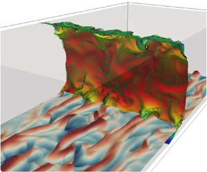
A rather rudimentary but insightful way to visualize fluid element deformation at a macroscopic level is through the evolution of initially planar material surfaces (Yeung Reference Yeung2002), which is provided directly by the reference map  $\boldsymbol {\xi }$. Specifically, we track how the tracers that form a constant streamwise and a constant wall-normal plane at
 $t=0$ evolve in response to the background turbulent flow. Note that this is essentially the 3-D counterpart of material-line tracking in figure 5. Figure 11 shows the time evolution of the plane identified by
 $\xi _1(x,y,z,t=0) = 1.5\delta$ from
 $t^{+}=0$ to
 $t^{+}=4$. It is interesting to note that the structures visible from the instantaneous velocity at
 $t^{+}=0$ leave a mark on the material surface as it evolves in time. Specifically, a mushroom structure indicative of a hairpin vortex is observed towards the top right of the plane. The regions of lower velocity within this structure lag behind the higher-velocity fluid particles outside it, leaving an imprint of the background turbulent flow structures on the material surface at
 $t^{+}=4$. In figure 11(c), the backward-time FTLE is plotted on the deformed
 $\xi _1(x,y,z,t)$ surface, showing that the imprinted structures correspond to regions of high FTLE.
Time evolution of the material surface corresponding to the constant streamwise plane  $x/\delta =1.5$ at
 $t^{+}=0$. The surface is evolved from (a)
 $t^{+}=0$ to (b)
 $t^{+}=4$, coloured by the instantaneous streamwise velocity. (c) shows the same material surface at
 $t^{+}=4$ coloured by the backward-time FTLE.

Figure 12 shows three material surfaces at  $t^{+}=8$ identified by the isosurfaces of
 $\xi _2$. Note that at
 $t=0$, these three material surfaces coincide with constant wall-normal planes at
 $y/\delta =-0.95$ (
 $y^{+}=10$),
 $y/\delta =-0.85$ (
 $y^{+}=30$) and
 $y/\delta =-0.61$ (
 $y^{+}=70$). These locations approximately lie in the viscous sublayer, buffer layer and log layer, respectively. The tracking of a material surface initialized at a constant wall-normal distance is particularly helpful in identifying flow structures that cause significant vertical motion of the fluid particles such as sweep and ejection events. Figures 12(a,d,g) show that the wall-normal deformation of the material surfaces gets stronger with increasing distance from the wall, which is perhaps an indication of the increasing eddy sizes away from the wall as per the attached-eddy hypothesis. Figures 12(b,e,h) show the same deformed surfaces now coloured with the streamwise velocity fluctuations. It is observed that the elevations and depressions of the material surfaces (in figures 12a,d,g) tend to correspond respectively with the regions of negative and positive
 $u'$ (in figures 12b,e,h), indicating the presence of ejection and sweep events. This becomes evident in figures 12(c, f,i), where
 $u'v'$ is plotted onto the deformed material surface. The strongly deformed regions (in figures 12a,d,g) are seen to correspond to regions of large negative
 $u'v'$ values (in figures 12c, f,i). Furthermore, the regions of negative
 $u'v'$ dominate all three layers next to the wall, but the buffer layer is most active in terms of these sweep and ejection events.
Identification of ejection and sweep events through the time-evolved material surfaces of constant  $\xi _2(x,y,z,t=0)$ at
 $t^{+}=8$. Each row corresponds to a different wall-normal plane from which
 $\xi _2(x,y,z,t=0)$ is initialized: (a–c)
 $y^{+}=10$, (d–f)
 $y^{+}=30$, (g–i)
 $y^{+}=70$. Plots in (a,d,g), (b,e,h) and (c, f,i) are coloured by
 $y/\delta$,
 $u'^+$ and
 $u'^+v'^+$, respectively.

To get a more holistic and consolidated picture of the flow structures identified individually from the  $x$- and
 $y$-plane tracking, in figure 13 we superimpose at
 $t^{+}=8$ the constant
 $\xi _1$ and constant
 $\xi _2$ surfaces initially at
 $x/\delta =2.4$ and
 $y/\delta =-0.85$, respectively. Furthermore, to show the relation of these structures to those from the
 $Q$-criterion, the velocity vectors coloured by the
 $Q$-criterion are plotted onto the deformed
 $\xi _1$ surface. We focus on one particular instance of a structure shown in the black box in figure 13(a). Here, the
 $\xi _2$ surface indicates the presence of an elongated low-speed streak through elevation in the material surface. Consistent with the well-studied mechanism for the low-speed streaks, this streak lies exactly between a pair of counter-rotating vortices depicted by the velocity vectors and the regions of high
 $Q$. The velocity vectors clearly show the ejection of fluid away from the wall between the two vortices. Furthermore, the lagging region of the
 $\xi _1$ surface (described above in relation to figure 11) also coincides with the low-speed streak, and is located between the counter-rotating vortex pair. The
 $\xi _1$ material surface exhibits twisting that is consistent with the direction of each of the counter-rotating vortices.
Time-evolved material surfaces at  $t^{+}=8$ corresponding to the initially constant streamwise plane
 $x/\delta =1.5$ and the initially constant wall-normal plane
 $y/\delta =-0.85$ (
 $y^{+}=30$) at
 $t^{+}=0$. The streamwise material surface is coloured by the instantaneous streamwise velocity, superimposed with the velocity vectors (coloured by
 $Q$). The wall-normal material surface is coloured with the wall-normal coordinate (
 $y/\delta$).

In summary, the tracking of material surfaces over short durations of time presents a simple but natural way of identifying instantaneous Lagrangian structures. It is noted that material surfaces are found to retain the initial topologically connected surface for considerable times commensurate with local-flow time scales. For instance, the time scale of eddies in the logarithmic region according to Lozano-Durán & Bae (Reference Lozano-Durán and Bae2019) is  $\kappa y^+$ (
 $\kappa \approx 0.4$). Consistent with this, the material surface in figure 14 initialized at
 $y^{+}=100$ in the log layer remains topologically connected up to approximately
 $t^{+} = 40$, implying that the current material surface tracking can be utilized usefully to study the Lagrangian dynamics of eddies therein.
Time evolution of the material surface initially corresponding to the constant  $y$-plane at
 $y^{+}=100$: (a)
 $t^{+}=8$, (b)
 $t^{+}=20$, (c)
 $t^{+}=40$, (d)
 $t^{+}=60$.

5. Discussion and conclusion
In this study, we have explored the application of the reference map technique, originally developed for the computation of solid stress in an Eulerian manner, to fluid mechanics within the context of Lagrangian kinematics. This approach is mathematically equivalent to the work of Leung (Reference Leung2011), who computed the flow map of simple two-dimensional (2-D) flows using an Eulerian approach. We discuss important modifications necessary for its application to complex three-dimensional (3-D) turbulent flows, including the conservative, low-dissipation update of the reference map, and treatment of periodic boundary conditions. Traditional methods for computing Lagrangian kinematics involve the explicit tracking of tracer particles forwards or backwards in time, allowing for the calculation of the flow map and its gradient on an auxiliary background grid. The reference map offers an alternative by enabling the calculation of these quantities without the use of particles. This is accomplished through the Eulerian update of the advection equation governing the evolution in time of the spatial distribution of the reference map. The reference map records the take-off positions of tracers arriving at fixed mesh points, effectively tracking tracer particles backwards in time, but in an implicit manner.
The reference map approach for Lagrangian kinematics offers enhanced flexibility and efficiency compared to the particle approach, particularly when the flow is derived through numerical simulation. The particle approach often necessitates seeding a substantial number of particles to reliably capture fluid particle trajectories across the flow domain seamlessly. The clustering of particles may result in the flow map (or its inverse) becoming a non-injective function, potentially leading to the ill-conditioning of the deformation gradient (Kafiabad Reference Kafiabad2022). Overall, the effective particle resolution surpasses that of the flow grid. When tracer trajectories are calculated on the fly with Navier–Stokes integration, this can result in a significant increase in computational cost, as well as additional overhead for large memory allocation. Achieving parallel load balancing of particles across processors can also pose challenges, especially when particle distribution in the processor space becomes highly irregular, as is often the case in inhomogeneous flows. The choice of an interpolation scheme to approximate particle velocity at non-mesh points is recognized to significantly impact the clarity of the Lagrangian structure (Kafiabad & Vanneste Reference Kafiabad and Vanneste2023). High-order schemes, recommended to be at least fourth-order accurate and twice continuously differentiable (e.g. cubic spline; Yeung Reference Yeung2002), play a crucial role in this regard. In contrast, the grid resolution for the reference map is inherently identical to that of the velocity and can be increased as needed. Load balancing is easily achieved with the standard domain decomposition already implemented for the flow solution. Velocity (or flux) data are consistently available at locations required by the reference map, eliminating the necessity for interpolation. The cost of the finite-time Lyapunov exponent (FTLE) field calculation appears to be competitively comparable to the particle-based approach, as demonstrated in figure 3.
The information implicitly embedded in the reference map regarding fluid particle trajectories provides a means to calculate measures of Lagrangian fluid element deformation solely from Eulerian data. These measures encompass displacement, deformation gradient tensor, and (left/right) Cauchy–Green tensor. They can be further leveraged to compute the backward-time FTLE field, with its ridges identified as candidates for the attracting Lagrangian coherent structure (LCS). We demonstrated the accuracy of FTLE calculations based on the reference map in comparison to the standard particle-based approach using a simple 2-D flow (2-D Taylor–Green vortex). The LCS detection utilizing the reference map was then applied to turbulent channel flow at  $Re_\tau = 180$. The computed LCSs exhibited consistency with structures identified through the
 $Q$-criterion, where the FTLE ridges closely approximated the boundaries of the
 $Q$-criterion structures, as illustrated in Green et al. (Reference Green, Rowley and Haller2007). A notable drawback of the current approach, in contrast to widely used Eulerian vortex identification schemes, is the high cost associated with incorporating an additional three advection equations for the reference map. While Eulerian schemes reveal coherent structures based on the instantaneous velocity field, an LCS based on the concept of finite-time dynamical systems necessitates fluid particle trajectories over a specified time interval. Given that dominant LCSs tend to converge over relatively short time scales (Green et al. Reference Green, Rowley and Haller2007; Huang et al. Reference Huang, Borthwick and Lin2022), this increased computational cost may be confined to a small fraction of the total simulation cost by integrating the reference map equation only during the time when it is needed.
While the reference map does not explicitly track a particle with a fixed label, its ability to return the take-off positions of tracers arriving at grid points makes it well suited for material surface tracking. Various shapes of material surfaces at the initial time can be realized through a judicious choice of the functional of the reference map. We have demonstrated the evolution of material surfaces with initial conditions set as streamwise constant or wall-normal constant planes in turbulent channel flow. This capability is notably unique to the reference map, as the reconstruction and visualization of equivalent surfaces with purely Lagrangian approaches are not straightforward. The time evolution of material surfaces provides valuable insights into the Lagrangian landscape of turbulent momentum transport, which remains obscured in the Eulerian velocity field. Figure 12, in a sense, can be considered as a visual Lagrangian quadrant analysis. Although it lacks quantitative information, it offers an immediate 3-D visual account of key events to be analysed through quadrant analysis. These events include ejections and sweeps identified from the vertical displacement of material surfaces, the signs and intensities of associated velocity fluctuations ( $u'$ and
 $v'$), the identification of low/high-speed streaks, and confirmation of the dominance of Reynolds-stress-generating events in the second and fourth quadrants.
In conclusion, this paper explores the application of the reference map technique (or equivalently the approach of Leung Reference Leung2011) to complex fluid flows, with a focus on the computation of LCSs, the tracking of material surfaces, and the analysis of turbulent momentum transport from a Lagrangian perspective, all in an Eulerian manner. It provides a convenient method and a promising direction for future investigations into Lagrangian kinematics and dynamics of fluid flows. One immediate application of the reference map technique could be in characterizing the deformation of Lagrangian fluid elements. For example, the deformation gradient fully characterizes the deformation of infinitesimal material lines as well as oriented material areas (Nanson's formula) (Gurtin et al. Reference Gurtin, Fried and Anand2010).
Funding
This research was sponsored by a faculty startup grant and the Ashton fellowship provided by the University of Pennsylvania.
Declaration of interests
The authors report no conflict of interest.
Appendix A. Duality between the backward- and forward-time FTLEs: proof of (2.12)
The largest forward-time FTLE at position  $\boldsymbol {X}$ is defined as
 \begin{equation} \varLambda^{t}_{t_0}(\boldsymbol{X}) = \frac{1}{|t - t_0|}\ln\sqrt{\lambda_{{max}}(\boldsymbol{C}^{t}_{t_0}(\boldsymbol{X}))}, \end{equation}
where  $\boldsymbol {C}^{t}_{t_0}(\boldsymbol {X}) = (\boldsymbol {F}^{t}_{t_0}(\boldsymbol {X}))^{\rm T}\boldsymbol {F}^{t}_{t_0}(\boldsymbol {X})$ is the right Cauchy–Green deformation tensor of the forward map. One can show from the chain rule that
 \begin{equation} \boldsymbol{F}^{t_0}_{t}(\boldsymbol{x})\,\boldsymbol{F}^{t}_{t_0}(\boldsymbol{X}) = \frac{\partial \boldsymbol{X}}{\partial \boldsymbol{x}}\,\frac{\partial \boldsymbol{x}}{\partial \boldsymbol{X}} = \boldsymbol{I}, \end{equation}
therefore  $\boldsymbol {F}^{t}_{t_0}(\boldsymbol {X}) = (\boldsymbol {F}^{t_0}_{t}(\boldsymbol {x}))^{-1}$. Using this result on the right Cauchy–Green tensor,
 \begin{align}
\boldsymbol{C}^{t}_{t_0}(\boldsymbol{X}) & = \big
[(\boldsymbol{F}^{t_0}_{t}(\boldsymbol{x}))^{{-}1}\big
]^{\rm
T}(\boldsymbol{F}^{t_0}_{t}(\boldsymbol{x}))^{{-}1}\nonumber\\
& = \left [(\boldsymbol{F}^{t_0}_{t}(\boldsymbol{x}))^{{\rm
T}}\right
]^{{-}1}(\boldsymbol{F}^{t_0}_{t}(\boldsymbol{x}))^{{-}1}\nonumber\\
& = \left
[\boldsymbol{F}^{t_0}_{t}(\boldsymbol{x})\,(\boldsymbol{F}^{t_0}_{t}(\boldsymbol{x}))^{{\rm
T}}\right ]^{{-}1}\nonumber\\ & = \left
[\boldsymbol{B}_{t}^{t_0}(\boldsymbol{x}) \right]^{{-}1},
\end{align}
where  $\boldsymbol {B}_{t}^{t_0}(\boldsymbol {x})$ is the left Cauchy–Green deformation tensor of the backward flow map. Thus we have
 \begin{equation} \lambda_{{max}}(\boldsymbol{C}^{t}_{t_0}(\boldsymbol{X})) = \frac{1}{\lambda_{{min}}(\boldsymbol{B}_{t}^{t_0}(\boldsymbol{x}))}. \end{equation}
Next, we show that the eigenvalues of  $\boldsymbol {B}_{t}^{t_0}(\boldsymbol {x})$ are equal to the eigenvalues of
 $\boldsymbol {C}_{t}^{t_0}(\boldsymbol {x})$. Let
 $\boldsymbol {r}$ be an eigenvector of
 $\boldsymbol {B}_{t}^{t_0}(\boldsymbol {x})$, with corresponding eigenvalue
 $\lambda$. Then
 \begin{equation} \boldsymbol{F}^{t_0}_{t}(\boldsymbol{x})\,(\boldsymbol{F}^{t_0}_{t}(\boldsymbol{x}))^{{\rm T}}\, \boldsymbol{r} = \lambda \boldsymbol{r}. \end{equation}
Pre-multiplying this relation by  $(\boldsymbol {F}^{t_0}_{t}(\boldsymbol {x}))^{{\rm T}}$,
 \begin{equation} \boldsymbol{C}_{t}^{t_0}(\boldsymbol{x})\,(\boldsymbol{F}^{t_0}_{t}(\boldsymbol{x}))^{{\rm T}}\, \boldsymbol{r} = \lambda (\boldsymbol{F}^{t_0}_{t}(\boldsymbol{x}))^{{\rm T}}\,\boldsymbol{r}. \end{equation}
Therefore,  $\lambda$ is also an eigenvalue of
 $\boldsymbol {C}_{t}^{t_0}(\boldsymbol {x})$ with eigenvector
 $(\boldsymbol {F}^{t_0}_{t}(\boldsymbol {x}))^{{\rm T}}\,\boldsymbol {r}$, so
 $\lambda _{{min}}(\boldsymbol {B}_{t}^{t_0}(\boldsymbol {x})) = \lambda _{{min}}(\boldsymbol {C}_{t}^{t_0}(\boldsymbol {x}))$. Using this result in (A4) gives
 \begin{equation} \lambda_{{max}}(\boldsymbol{C}^{t}_{t_0}(\boldsymbol{X})) = \frac{1}{\lambda_{{min}}(\boldsymbol{B}_{t}^{t_0}(\boldsymbol{x}))} = \frac{1}{\lambda_{{min}}(\boldsymbol{C}_{t}^{t_0}(\boldsymbol{x}))} = \frac{1}{\lambda_{{min}}(\boldsymbol{C}_{t}^{t_0}(\boldsymbol{\chi}^{t}_{t_0}(\boldsymbol{X})))}. \end{equation}
Substituting this result into (A1) produces the duality relation in (2.12):
 \begin{align} \varLambda^{t}_{t_0}(\boldsymbol{X}) & = \frac{1}{|t - t_0|}\ln\sqrt{\lambda_{{max}}(\boldsymbol{C}^{t}_{t_0}(\boldsymbol{X}))}\nonumber\\ & = \frac{1}{|t - t_0|}\ln\left[ \lambda_{{min}}(\boldsymbol{C}_{t}^{t_0}(\boldsymbol{\chi}^{t}_{t_0}(\boldsymbol{X}))) \right]^{{-}1/2}\nonumber\\ & ={-}\frac{1}{|t - t_0|}\ln\left[ \lambda_{{min}}(\boldsymbol{C}_{t}^{t_0}(\boldsymbol{\chi}^{t}_{t_0}(\boldsymbol{X}))) \right]^{1/2}\nonumber\\ & ={-} \varGamma^{t_0}_t(\boldsymbol{\chi}^{t}_{t_0}(\boldsymbol{X})). \end{align}
The utility of this equation is as follows. In the reference map approach, the smallest backward-time FTLE can be first computed in the current configuration (or the grid) ( $\varGamma ^{t_0}_t(\boldsymbol {x})$). The negative of this can be considered as the largest forward-time FTLE (
 $\varLambda ^{t}_{t_0}$), graphed not on
 $\boldsymbol {X}$ but on the forward-flow image of
 $\boldsymbol {X}$. If
 $\varLambda ^{t}_{t_0}$ needs to be graphed on
 $\boldsymbol {X}$, then
 $\boldsymbol {X} = \boldsymbol {\xi }(\boldsymbol {x}, t)$ can be used in principle to build the initial/reference configurations
 $\boldsymbol {X}$.


 Open access

