1. Introduction
Numerical simulation is an increasingly important component of both academic and engineering investigations of turbulence, which is a near-ubiquitous phenomenon in compressible flow regimes, including aerodynamics and turbo-machinery. Compared to the low-speed incompressible regime, the computational fluid dynamics of high-speed compressible flows is further complicated by the significant variation of density and thermodynamic fluid properties. Though results from direct numerical simulation (DNS) of the compressible Navier–Stokes equations provide tremendous insight, this approach remains prohibitively expensive even for moderately sized problems, mainly due to the vast range of spatial and temporal scales that are involved in turbulent flows of scientific and engineering interest. Many alternative approaches are practically used to make the simulation of turbulence feasible, including coarser resolution approximation and dynamic adaptation. In particular, the adaptive wavelet collocation (AWC) method has been demonstrated as an effective computational tool, forming a cogent framework for turbulence simulation that exploits a greatly reduced memory footprint (Schneider & Vasilyev Reference Schneider and Vasilyev2010). Sharing properties with the adaptive mesh refinement (AMR) procedure, wavelet-based methods seek to exploit the characteristic spatio-temporal intermittency of turbulence by maintaining a sparse data representation, thereby lowering the computational cost of simulations. Owing to the automatic adaptation process, the spatial mesh in the regions of slowly varying flow fields is coarsened, while zones with steep gradients and highly energetic localized structures become more refined. Moreover, a distinguishing advantage of wavelet-based methods is that they provide a priori highly controlled error and well-behaved adjustable numerical accuracy (Vasilyev, Yuen & Paolucci Reference Vasilyev, Yuen and Paolucci1997; Vasilyev Reference Vasilyev2003).
Wavelet-based adaptive large-eddy simulation (WA-LES) is a computational approach that combines the tenets and benefits of wavelet-based adaptive turbulence simulation with the traditional large-eddy simulation (LES) method, whereby a filtered form of the governing equations is solved using relatively coarse adaptive grids (Goldstein & Vasilyev Reference Goldstein and Vasilyev2004). In the classical LES approach, a low-pass filter is utilized to reduce the computational complexity of the constitutive equations. With sufficient separation between integral and dissipative length scales, the residual smaller turbulent eddies within the inertial subrange are assumed to take on some universal character, whose influence can be deduced from the resolved modes based upon scaling arguments (e.g. Germano et al. Reference Germano, Piomelli, Moin and Cabot1991). Basically, the retained large scales are presumed to capture the distinctive behaviour of particular flow configurations and are directly simulated, while modelling the effect of subgrid-scale (SGS) motions. Analogously, the WA-LES method exploits a wavelet filter to construct an LES-like approximation on adaptive computational meshes. However, while traditional low-pass filtering splits the turbulent fields into large- and small-scale flow structures, the wavelet filter decomposes them into coherent/incoherent and more/less energetic components, based on a specified wavelet thresholding level. The incoherent and the less energetic coherent portions of the turbulent fields across all length scales are discarded in the simulation, while assuming that the effect of the residual modes on the resolved flow dynamics has a sufficiently universal character to be captured by generalized closure models. Where this assumption might fail, the above effect is minimized since the wavelet-based SGS modes represent, by definition, the lowest relative energy content. Taking into account that unresolved small-scale coherent structures are largely responsible for the SGS dissipation in LES, while the majority of incoherent SGS motions negligibly contribute to the total energy transfer (De Stefano, Goldstein & Vasilyev Reference De Stefano, Goldstein and Vasilyev2005), many standard closure procedures have been successfully extended to the incompressible WA-LES framework, including various eddy-viscosity-type approaches (Goldstein, Vasilyev & Kevlahan Reference Goldstein, Vasilyev and Kevlahan2005; De Stefano, Vasilyev & Goldstein Reference De Stefano, Vasilyev and Goldstein2008; Vasilyev et al. Reference Vasilyev, De Stefano, Goldstein and Kevlahan2008).
While it might seem that WA-LES simply represents a different form of LES that utilizes a different filtering procedure, the underlying physical mechanisms behind the two approaches are, in fact, drastically different. In contrast to classical LES, which resolves large-scale motions, WA-LES focuses on capturing energetic coherent flow structures, which are either totally or partially resolved. The method sometimes necessitates local higher mesh resolution in order to correctly capture the energy cascade within resolved coherent structures. Therefore, filtering, adaptive gridding and computational environments are all tightly coupled within the WA-LES methodology. Calculations occur on adaptive grids that are automatically refined or coarsened following the evolution of transient dynamically important flow structures. Moreover, in addition to optimizing the computational complexity, by controlling the quality of mesh and spatial discretization for optimal representation of coherent energetic structures, WA-LES fully exploits the characteristic spatio-temporal intermittency of the turbulent energy cascade, resulting in few occurrences of higher local resolution. This fact was evidenced by the high grid compression practically obtained in previous incompressible studies and is confirmed here for compressible flows.
Within the wavelet-based eddy-resolving simulation hierarchy, WA-LES is the lowest-fidelity approach, as the unresolved SGS modes substantially influence the dynamics of resolved motions. In addition to the stochastic/incoherent content that is discarded in coherent vortex simulation (CVS), WA-LES also removes the lowest-energy coherent modes (Goldstein et al. Reference Goldstein, Vasilyev and Kevlahan2005). An explicit closure model is therefore necessary, since the effect of coherent unresolved SGS modes is non-negligible (De Stefano etal. Reference De Stefano, Goldstein and Vasilyev2005). Furthermore, the complete or partial removal of dissipative length scales necessitates additional mechanisms for the dissipation of resolved turbulent kinetic energy. While WA-LES is not predicated on a specific class of closure procedures, certain SGS modelling properties are particularly advantageous in this framework. By employing models that automatically switch off in well-resolved flow regions, the control of the overall physical fidelity can be achieved by means of the adaptive wavelet-based filtering procedure (De Stefano & Vasilyev Reference De Stefano and Vasilyev2014), thereby forming a completely unified eddy-resolving modelling framework, capable of continuously changing between WA-LES, CVS and wavelet-based adaptive direct numerical simulation (WA-DNS) regimes, within a single simulation. The filtering parameters can be automatically adjusted, both spatially and temporally, based on objective physically based criteria throughout the course of the simulation, while targeting specific flow phenomena, which leads to the intelligent simulation of turbulent flows (Nejadmalayeri et al. Reference Nejadmalayeri, Vezolainen, De Stefano and Vasilyev2014; De Stefano, Nejadmalayeri & Vasilyev Reference De Stefano, Nejadmalayeri and Vasilyev2016). As the filtering parameters are tightened, a greater portion of the turbulent fields is retained and resolved, while lessening the effect of the SGS model, which eventually becomes negligible.
Though the wavelet-based turbulence simulation framework has been shown to be very promising, its development has been mostly within the context of incompressible turbulence. A few authors have considered the low-Mach-number regime of compressible transport equations, for instance, investigating CVS of mixing layers (Roussel & Schneider Reference Roussel and Schneider2010). Furthermore, research has been limited to a relatively narrow set of configurations, including homogeneous isotropic turbulence (Goldstein et al. Reference Goldstein, Vasilyev and Kevlahan2005; De Stefano & Vasilyev Reference De Stefano and Vasilyev2010), as well as turbulent wake flows behind bluff bodies (De Stefano & Vasilyev Reference De Stefano and Vasilyev2014; De Stefano et al. Reference De Stefano, Nejadmalayeri and Vasilyev2016). Though the latter feature bounded flows, the Reynolds number was in the transitional regime and the boundary layer remained laminar.
In this work, the WA-LES approach is originally extended to the computational modelling of shock-free wall-bounded compressible turbulent flows, where variable density and thermodynamic effects are important. The governing equations consist of the wavelet-filtered compressible Navier–Stokes equations, complemented by SGS models for the unclosed terms. Turbulent eddy-viscosity and eddy-conductivity modelling procedures are developed following the anisotropic minimum-dissipation (AMD) approach of Rozema et al. (Reference Rozema, Bae, Moin and Verstappen2015). The AMD model is chosen for its low computational cost in both memory and complexity. Minimum-dissipation models seek to approximate the least eddy-viscosity and eddy-diffusivity coefficients necessary to prevent the formation of structures smaller than the local numerical grid. The overall computational modelling procedure is validated for the simulation of supersonic turbulent channel flow with isothermal walls. The present configuration examines the behaviour of the novel compressible WA-LES method in a case where fully developed turbulent flow conditions exist. In order to more efficiently resolve the wall region, the adaptive anisotropic wavelet collocation (A-AWC) method (Brown-Dymkoski & Vasilyev Reference Brown-Dymkoski and Vasilyev2017) is used, permitting appropriate stretching of the wavelet-based spatial mesh in the wall-normal direction.
The remainder of this paper is organized as follows. In § 2, the AWC method is briefly reviewed. The new wavelet-based adaptive compressible LES approach is introduced in § 3, where the governing equations are presented together with the closure modelling procedure. The results of the numerical experiments for supersonic turbulent plane channel flow are made known and discussed in § 4. Finally, some concluding remarks are drawn in § 5.
2. Wavelet-based adaptive collocation method
The AWC method is a multi-resolution approach that uses a wavelet threshold filtering (WTF) procedure to dynamically adapt the discrete numerical grid to physical features in the solution. The filter acts by decomposing a discrete scalar field into a set of bi-orthogonal wavelet basis functions. Wavelet functions have many attractive properties for multi-resolution analysis as they have localized support in both wavenumber and physical space, due to vanishing moments and rapid spatial decay, respectively. In comparison, the Fourier transform provides precise information about the frequency content of a signal, but gives no spatial insight, due to the global support of the Fourier modes. While there are several classes of wavelets that are suitable for the solution of partial differential equations, in this work, second-generation interpolating wavelets have been implemented, due to computational efficiency (Sweldens Reference Sweldens1998) and previous development of the parallel AWC method (Nejadmalayeri et al. Reference Nejadmalayeri, Vezolainen, Brown-Dymkoski and Vasilyev2015).
In the wavelet transform, a general scalar field variable, say  $u(\boldsymbol {x})$, is discretized by a series of dyadic nested grids comprising collocation points on different resolution levels. Specifically, the unfiltered variable can be represented by the series
 \begin{equation} u(\boldsymbol{x}) = \sum_{ {\boldsymbol{l}} \in \mathcal{L}^0} c_{ \boldsymbol{l}}^{0} \phi_{ \boldsymbol{l}}^{0}(\boldsymbol{x}) + \sum_{j=1}^{+\infty} \sum_{\mu=1}^{2^n-1} \sum_{{ \boldsymbol{k}} \in \mathcal{K}^{\mu,j}} d_{{ \boldsymbol{k}}}^{\mu,j} \psi_{{ \boldsymbol{k}}}^{\mu,j}(\boldsymbol{x}), \end{equation}
where  $\phi _{{\boldsymbol {l}}}^{0}$ and
 $\psi _{{\boldsymbol {k}}}^{\mu ,j}$ represent
 $n$-dimensional tensor product scaling functions and wavelets of different families (indexed by
 $\mu$) and resolution levels (indexed by
 $j$). The bold subscripts
 $\boldsymbol {l}$ and
 $\boldsymbol {k}$ denote
 $n$-dimensional indices, while
 $\mathcal {L}^0$ and
 $\mathcal {K}^{\mu ,j}$ stand for the associated index sets. The scaling functions
 $\phi _{\boldsymbol {l}}^{0}$ carry the averaged signal, while the wavelet functions
 $\psi _{{\boldsymbol {k}}}^{\mu ,j}$ define the local variational details. The corresponding amplitudes are given by the coefficients
 $c_{\boldsymbol {l}}^{0}$ and
 $d_{{\boldsymbol {k}}}^{\mu ,j}$, respectively, and likewise have a unique correspondence to grid points
 $\boldsymbol {x}_{{\boldsymbol {k}}}^j$. For an arbitrary
 $n$-dimensional space, there are
 $2^n-1$ different families of wavelet functions. Each level of resolution consists of families of wavelets
 $\psi _{{\boldsymbol {k}}}^{\mu ,j}$ having the same scale but located at different grid positions.
The WTF operation arises naturally from the series expansion (2.1) if wavelets with coefficients falling below some prescribed limit are discarded. Therefore, the corresponding wavelet-filtered quantity, say  ${\bar {u}^{{>}\epsilon }}(\boldsymbol {x})$, can be represented by the conditional series
 \begin{equation} {\bar{u}^{{>}\epsilon }}(\boldsymbol{x}) = \sum_{ {\boldsymbol{l}} \in \mathcal{L}^0} c_{ \boldsymbol{l}}^{0} \phi_{ \boldsymbol{l}}^{0}(\boldsymbol{x}) + \sum_{j=1}^{J} \sum_{\mu=1}^{2^n-1} \sum_{ \substack{{\boldsymbol{k}} \in \mathcal{K}^{\mu,j}\\ |d_{{\boldsymbol{k}}}^{\mu,j}| \geq \epsilon \lVert u \rVert_{{WTF}}}} d_{{ \boldsymbol{k}}}^{\mu,j} \psi_{{ \boldsymbol{k}}}^{\mu,j}(\boldsymbol{x}), \end{equation}
whose terms are a subset of (2.1). Practically, the filtered variable consists of the relatively more important modes, given the number of resolution levels  $J$. The non-dimensional positive parameter
 $\epsilon$ determines the relative level of thresholding, while the absolute threshold is taken to be proportional to some characteristic signal amplitude, which is represented by
 $\lVert u \rVert _{{WTF}}$ in the above definition. Once the norm
 $\lVert \cdot \rVert _{{WTF}}$ is specified, the spatial filtering operator (2.2) is uniquely defined by the constant parameter
 $\epsilon$. In this work, following usual implementations, the
 $L_2$-norm of the wavelet filtered solution is used, namely
 $\lVert \cdot \rVert _{{WTF}} \equiv \lVert \cdot \rVert _2$ (e.g. Goldstein & Vasilyev Reference Goldstein and Vasilyev2004). For a properly normalized threshold
 $\epsilon$, the reconstruction error of the filtered variable was shown to converge according to
 \begin{equation} { \lVert u - {\bar{u}^{{>}\epsilon }} \rVert_2} \le \mathcal{C} \epsilon {\lVert u \rVert_2 } , \end{equation}
where  $\mathcal {C}$ is a constant of order unity (Donoho Reference Donoho1992). Therefore, the wavelet-based approach provides highly controlled a priori error estimation.
It is worth noting that the WTF operation is actually nonlinear. The dynamic adaptation of the grid is tightly coupled to the wavelet filter, resulting from the localization of wavelet functions in computational space, and their one-to-one correspondence to grid nodes. As modes are filtered out, their respective collocation points are omitted from the spatial grid, because the associated value of  ${\bar {u}^{{>}\epsilon }}$ can be reconstructed (interpolated) using the retained wavelet functions. The resulting sparse grid exactly reconstructs the filtered field (2.2). It should be noted that the wavelet filter, and therefore the wavelet-based interpolation, is not positivity preserving. Since the wavelet modes capture high local energy, the grid is clustered and more refined around strong structures in the flow field, while becoming coarser in regions of low variation. Adaptation for transient signals is accomplished by predicting collocation points that may become significant in the next time step or iteration, as the wavelet filter only acts to remove points. The sparse grid, supporting
 ${\bar {u}^{{>}\epsilon }}$, is augmented by adding the nearest neighbours to every significant collocation point on the current, next higher and next lower resolution levels. This reflects a Courant–Friedrichs–Lewy (CFL) type (Courant, Friedrichs & Lewy Reference Courant, Friedrichs and Lewy1928) argument for the finite-rate transfer of information, both spatially and with respect to wavenumbers. The successive application of wavelet filtering and grid adaptation across time effectively tracks and maintains resolution of the important flow structures during their evolution. For fluid flow systems that have multiple quantities of interest, given the relative level of thresholding, each field is filtered separately, with the associated absolute threshold, and solved on the union of corresponding collocation grids. This permits the use of control and proxy variables to ensure that all the desired aspects of the solution are maintained for a prescribed fidelity of the simulation and associated analyses.
Furthermore, as opposed to wavelet Galerkin methods, the AWC method solves the governing equations in real space. In this work, derivative approximations are provided by central fourth-order finite differences at the local adaptive resolution level. Where differencing stencil points do not explicitly exist on the current adaptive wavelet grid, the functional values are interpolated from the underlying wavelet basis functions. A full description of the numerical algorithms can be found, for instance, in Vasilyev & Bowman (Reference Vasilyev and Bowman2000), Paolucci, Zikoski & Wirasaet (Reference Paolucci, Zikoski and Wirasaet2014) and Nejadmalayeri et al. (Reference Nejadmalayeri, Vezolainen, Brown-Dymkoski and Vasilyev2015). While the second-generation wavelet basis used in this study requires a topologically regular, rectilinear grid, the consequent geometric restriction was recently obviated by developing the A-AWC method (Brown-Dymkoski & Vasilyev Reference Brown-Dymkoski and Vasilyev2017). This extension of the methodology permits the use of curvilinear mesh geometries, when appropriate, in order to optimize the computational cost of the simulation. Within this framework, however, the characteristic error control described above is preserved.
3. Wavelet-based compressible large-eddy simulation
The proposed compressible WA-LES method effectively leverages both the inherent spatial filtering and the dynamic adaptivity of the wavelet-based numerical procedure described above. The use of wavelets is not limited here to the efficient solution of the modelled equations by employing wavelet-based adaptive grids. This would occur for low-fidelity approaches such as Reynolds-averaged Navier–Stokes turbulence modelling procedures (De Stefano, Vasilyev & Brown-Dymkoski Reference De Stefano, Vasilyev and Brown-Dymkoski2018), where significant computational savings are achieved from wavelet-based grid compression. Differently, the present approach exploits the built-in filtering effect of the AWC method, the modelled equations being directly dependent on the WTF definition (2.2). As an alternative to the implicit filtering approach, one could consider two different levels of filtering, by superimposing an additional explicit wavelet filtering operation during the solution process (De Stefano & Vasilyev Reference De Stefano and Vasilyev2013). In that case, the turbulent scalar field to be solved for would still be  ${\bar {u}^{{>}\epsilon }}$, while the explicit filtering procedure is just a tool that makes it possible to use a lower thresholding level for the numerical grid adaptation. However, the use of such an approach would result in adding extra computational modes beyond the ones that are strictly necessary to achieve the prescribed turbulence resolution. In the present case of purely implicit filtering, the level of thresholding controls both the numerical accuracy and the LES filter resolution, because the adapted collocation grid in physical space, corresponding to the retained wavelets in computational space, is used to distinguish between the relative energy content of the localized flow structures and to identify their scale.
3.1. Governing equations
The governing equations for compressible WA-LES are formally obtained by applying the WTF procedure (2.2) to the following balance equations for mass, momentum and total energy:
 \begin{gather} \frac{\partial \rho}{\partial t} + \frac{\partial}{\partial x_j} ( \rho u _{j} ) = 0, \end{gather}
 \begin{gather}\frac{\partial }{\partial t} (\rho u_{i}) + \frac{\partial }{\partial x_j} ( \rho u_{i} u_{j} + p \delta_{ij} - \sigma_{ij} ) = 0, \end{gather}
 \begin{gather}\frac{\partial }{\partial t} (\rho e) + \frac{\partial }{\partial x_j} [ (\rho e + p) u_{j} - \sigma_{ij} u_i + q_j ]= 0. \end{gather}
Here the summation convention for repeated indices is used, while  $\delta _{ij}$ stands for the Kronecker delta. The viscous stress tensor in (3.2) is given by
 $\sigma _{ij} = 2 \mu S_{ij}^{*}$, where the superscript asterisk denotes the deviatoric part, that is,
 \begin{equation} S_{ij}^{*} = S_{ij} - \tfrac{1}{3}S_{kk}\delta_{ij}, \end{equation}
of the strain-rate tensor,
 \begin{equation} S_{ij} = \frac{1}{2}\left( \frac{\partial u_i}{\partial x_j} + \frac{\partial u_j}{\partial x_i} \right). \end{equation}
The molecular dynamic viscosity is assumed dependent on temperature,  $\mu = \mu (T)$, according to Sutherland's law. The thermodynamic state of the fluid is determined by the ideal-gas equation
 \begin{equation} p = \rho R T, \end{equation}
where  $R$ is the specific gas constant. The fluid is assumed as a calorically perfect gas with specific heat at constant pressure
 $c_p = \gamma R/(\gamma -1)$, with
 $\gamma$ being the ratio of specific heats. In (3.3), the total energy (per unit volume) is defined as the sum of internal and kinetic energy, namely
 \begin{equation} \rho e = \frac {p}{\gamma -1} + \frac 1 2 {\rho} u_{ i} u_{ i}, \end{equation}
while the heat flux is prescribed as
 \begin{equation} q_j = - \kappa \frac {\partial T}{\partial x_j}, \end{equation}
with the thermal conductivity being assumed dependent on temperature,  $\kappa = \kappa (T)$.
As usual for compressible LES, the governing equations are written in terms of density-weighted Favre-filtered variables. In this study, the Favre-filtering operator  $\widetilde {(\cdot )}$ is defined in conjunction with the WTF operator
 ${\overline {(\cdot )}^{{>}\epsilon }}$ as follows:
 \begin{equation} \tilde{\varphi} = \frac{{\overline{\rho \varphi}^{{>}\epsilon }}}{{\bar{\rho}^{{>}\epsilon }}},\end{equation}
where  $\varphi$ stands for a generic flow-field variable. By wavelet filtering the continuity equation (3.1) and the momentum equation (3.2), while assuming that the filtering operation commutes with temporal and spatial derivatives, the following filtered equations are obtained:
 \begin{gather} \frac{\partial {\bar{\rho}^{{>}\epsilon }}}{\partial t} + \frac{\partial}{\partial x_j} ( {\bar{\rho}^{{>}\epsilon }} \tilde{u} _{j} ) = 0, \end{gather}
 \begin{gather}\frac{\partial }{\partial t} ({\bar{\rho}^{{>}\epsilon }} \tilde{u}_{i}) + \frac{\partial }{\partial x_j} ( {\bar{\rho}^{{>}\epsilon }} \tilde{u}_{i} \tilde{u}_{ j} + {\bar{p}^{{>}\epsilon }} \delta_{ij} - \hat \sigma_{i j} + \tau_{i j} ) = 0 . \end{gather}
The resolved viscous stress tensor is given by  $\hat \sigma _{ij} = 2 \tilde {\mu } \tilde {S}_{ij}^{*}$, where
 $\tilde {\mu } = \mu (\tilde {T})$ and
 \begin{equation} \tilde{S}_{ij} = \frac{1}{2}\left( \frac{\partial \tilde{u}_i}{\partial x_j} + \frac{\partial \tilde{u}_j}{\partial x_i} \right) \end{equation}
stands for the filtered rate-of-strain tensor. Owing to the Favre-filtering approach, the filtered continuity equation (3.10) does not involve any unclosed term, whereas the SGS stresses in (3.11) are defined as
 \begin{equation} \tau_{ij}= {\bar{\rho}^{{>}\epsilon }} ( \widetilde{u_i u_j} - \tilde{u}_i\tilde{u}_j). \end{equation}
Note that, in deriving the filtered momentum equation (3.11), the residual term  ${\partial ( {\bar {\sigma }^{{>}\epsilon }}_{ij} - \hat \sigma _{ij} ) }/{\partial x_j}$ has been omitted as is usually done (Lenormand, Sagaut & Ta Phuoc Reference Lenormand, Sagaut and Ta Phuoc2000a), according to the results of a priori analysis (Vreman, Geurts & Kuerten Reference Vreman, Geurts and Kuerten1995).
A number of different formulations exist in the literature for the filtered energy equation (e.g. Martín, Piomelli & Candler Reference Martín, Piomelli and Candler2000; Lesieur, Métais & Comte Reference Lesieur, Métais and Comte2005). Here, this equation is written in terms of the resolved-scale total energy
 \begin{equation} {{\bar{\rho}^{{>}\epsilon }} }\hat e = \frac {{\bar{p}^{{>}\epsilon }}}{\gamma -1} + \frac 1 2 {{\bar{\rho}^{{>}\epsilon }}} \tilde{u}_{ i} \tilde{u}_{ i} , \end{equation}
which is the sum of filtered internal energy and the kinetic energy of the resolved velocity field (Vreman, Geurts & Kuerten Reference Vreman, Geurts and Kuerten1997). The transport equation for the energy variable (3.14) can be written as
 \begin{align} &\frac{\partial }{\partial t} ( {\bar{\rho}^{{>}\epsilon }} \hat e) + \frac{\partial}{\partial x_j} [ ( {\bar{\rho}^{{>}\epsilon }} \hat e + {\bar{p}^{{>}\epsilon }} ) \tilde{u}_{ j} - \hat \sigma_{ij} \tilde{u}_{i} + \hat q_j ] \nonumber\\ &\quad= -\alpha_1-\alpha_2-\alpha_3 +\alpha_4, \end{align}
where  $\hat q_j = -\tilde {\kappa } ({\partial \tilde {T}}/{\partial x_j})$, with
 $\tilde {\kappa } = \kappa (\tilde {T} )$, stands for the resolved heat flux. The residual SGS terms on the right-hand side of (3.15) are given by
 \begin{gather} \alpha_1 = \tilde{u}_i \frac{\partial \tau_{ij}}{\partial x_j}, \end{gather}
 \begin{gather}\alpha_2 = \frac 1 {\gamma -1} \frac{\partial}{\partial x_j} ( {\overline{p u_j}^{{>}\epsilon }} - {\bar{p}^{{>}\epsilon }} \tilde u_j ) , \end{gather}
 \begin{gather}\alpha_3 = {\overline{p \frac{\partial u_j}{\partial x_j}}^{{>}\epsilon }} - {\bar{p}^{{>}\epsilon }} \frac{\partial \tilde{u}_{j}}{\partial x_j} , \end{gather}
 \begin{gather}\alpha_4 = {\overline{\sigma_{ij} \frac{\partial u_i}{\partial x_j}}^{{>}\epsilon }} - {\bar{\sigma}^{{>}\epsilon }}_{ij} \frac{\partial \tilde{u}_{i}}{\partial x_j}. \end{gather}
Note that, in deriving the filtered energy equation (3.15), the residual terms  $({\partial }/{\partial x_j}) ( {\bar {\sigma }^{{>}\epsilon }}_{ij} \tilde {u}_i - \hat \sigma _{ij} \tilde {u}_i )$ and
 $({\partial }/{\partial x_j}) ( {\bar {q}^{{>}\epsilon }}_{j} - \hat q_{j} )$ have been omitted, as is usually done (Lenormand et al. Reference Lenormand, Sagaut and Ta Phuoc2000a), according to the results of a priori analysis (Vreman et al. Reference Vreman, Geurts and Kuerten1995). Finally, the compressible LES equations are supplemented by the following filtered version of the ideal-gas equation:
 \begin{equation} {\bar{p}^{{>}\epsilon }} = {\bar{\rho}^{{>}\epsilon }}R\tilde{T}. \end{equation}
It should be emphasized that, while the WA-LES governing equations are formally similar to standard LES equations, due to the local low-pass character of the WTF operation (2.2), the physical interpretation of the filtered equations is rather different, because of the substantial difference between wavelet-threshold and classical low-pass filtering. In contrast to standard LES equations that describe the evolution of large-scale motions, the WA-LES equations (3.10), (3.11) and (3.15) describe the evolution of energetic coherent structures. Also, differently from classical LES, the energy cascade within coherent structures is captured in WA-LES, which necessitates the use of adaptive gridding, where the local resolution is determined by the prescribed wavelet threshold. The latter parameter represents the counterpart of the mesh spacing or filter width parameter defined in classical LES.
3.2. Closure modelling
The compressible regime substantially increases the complexity of WA-LES, as the turbulent velocity field is influenced by thermodynamic variations and non-constant density. The inclusion of the energy transport equation (3.15) increases the number of nonlinear filtered terms that must be modelled, compared to the incompressible case. However, the use of the ideal-gas equation (3.20), in lieu of nonlinear real-gas equations of state, greatly simplifies the analysis. With the more complicated physical environment, the options for adaptive markers are greatly increased for compressible flows. A natural implementation, which is used in this work, corresponds to adapt on all balanced variables that are  ${\bar {\rho }^{{>}\epsilon }}$,
 ${\bar {\rho }^{{>}\epsilon }} \widetilde {u_i}$ and
 ${\bar {\rho }^{{>}\epsilon }}\hat e$, though this approach might be suboptimal for some flow configurations, since characteristic amplitude scales and flow phenomena of interest are highly dependent upon the particular case that is considered. Basically, the WA-LES framework for high-speed turbulence simulations requires targeted adaptation on the momentum components as well as any flow quantity driving important thermodynamic effects. For the present numerical experiments, also based upon previous studies on similar flow configurations, the temperature field is additionally used as sensor for the adaptive wavelet filter.
The specification of the threshold parameter  $\epsilon$ in the WTF definition (2.2) rigorously controls the filtering level in (3.9) and, therefore, the fidelity of the WA-LES solution. As previously discussed, apart from controlling the numerical error and thus the accuracy of the solution, the AWC method also filters out turbulent eddies based on their energetic level, regardless of their size. For vanishing threshold, the unclosed SGS terms approach zero and the filtered transport equations (3.10), (3.11) and (3.15) converge to their unfiltered counterparts (3.1)–(3.3). That is, the reconstruction error in (2.3) becomes negligible and the direct solution of the unfiltered equation is practically achieved. In the present case, with the use of an effective threshold, the lowest-energy motions are discarded in the simulation and the influence of the unknown residual terms needs to be approximated. The basic idea behind compressible WA-LES is that the resolved most-energetic modes dominate mixing, heat transfer and other quantities of interest, while the unresolved least-energetic modes are considered to be the most universal and permissive of generalized SGS modelling. Because the coherent part of the SGS turbulent quantities dominates the impact of unresolved motions upon the resolved fields (De Stefano et al. Reference De Stefano, Goldstein and Vasilyev2005), deterministic closure models, as those provided in the following, are presumed to mimic the effect of unclosed terms in the filtered governing equations. Also, preferable modelling approaches assume automatic convergence to unfiltered equations where the flow is well resolved, as this allows for implementing a unified eddy-resolving wavelet-based modelling framework, whereby WA-LES is able to locally revert to highly accurate CVS and WA-DNS, solely through the control of the AWC filtering mechanism.
In this work, the classical eddy-viscosity modelling approach is used, where the SGS modes in the filtered momentum equation (3.11) are considered to behave as additional dissipative forces, whose strength can be deduced from the resolved scales. The following approximation is employed for the anisotropic part of the SGS stress tensor (3.13),
 \begin{equation} \tau_{ij}^* \cong -2 \mu_e \tilde{S}_{ij}^*, \end{equation}
where  $\mu _e = {\bar {\rho }^{{>}\epsilon }}\nu _e$, with
 $\nu _e$ being the eddy-viscosity coefficient to be determined. The isotropic part of the SGS stress tensor is not explicitly modelled. The same approximation is exploited to model the unknown SGS term
 $\alpha _1$ (3.16) in the filtered energy equation (3.15). Following other LES studies (Moin et al. Reference Moin, Squires, Cabot and Lee1991; Lenormand et al. Reference Lenormand, Sagaut and Ta Phuoc2000a), the sum of the two SGS terms
 $\alpha _2$ (3.17) and
 $\alpha _3$ (3.18) is modelled by the divergence of the SGS heat flux vector field,
 \begin{equation} \mathcal{Q}_j = {\bar{\rho}^{{>}\epsilon }} c_p ( \widetilde{T u_j} - \tilde{T}\tilde{u}_j), \end{equation}
to be parametrized. Here, the eddy-conductivity model is employed to approximate the above unknown variable, namely
 \begin{equation} \mathcal{Q}_j \cong - \kappa_e \frac{\partial\tilde{T}}{\partial x_j}, \end{equation}
where  $\kappa _e$ stands for the eddy-conductivity coefficient to be determined. However, differently from other compressible LES works, where a constant turbulent Prandtl number
 ${Pr}_t$ is introduced so that
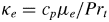 $\kappa _e = c_p \mu _e / {Pr}_t$, the eddy-conductivity coefficient is independently evaluated as discussed in the following. No model is introduced for the SGS term
 $\alpha _4$ (3.19) that is the SGS turbulent dissipation rate.
To assess the validity of the proposed compressible WA-LES approach, in this work, the numerical simulation of turbulent plane channel flow is performed. In order to yield fully developed flow conditions, an external body force is applied in the homogeneous streamwise direction (Huang, Coleman & Bradshaw Reference Huang, Coleman and Bradshaw1995), say  $x_1$. This way, also due to the modelling assumptions introduced above, the filtered momentum and energy equations that are solved can be written as
 \begin{gather} \frac{\partial }{\partial t} ( {\bar{\rho}^{{>}\epsilon }} \tilde{u}_{i} )+ \frac{\partial }{\partial x_j} [{\bar{\rho}^{{>}\epsilon }} \tilde{u}_{i} \tilde{u}_{ j} + {\bar{p}^{{>}\epsilon }} \delta_{ij} - 2 ( \tilde{\mu} + \mu_e ) \tilde{S}^*_{ij} ] = f \delta_{i1}, \end{gather}
 \begin{gather}\frac{\partial }{\partial t} ( {\bar{\rho}^{{>}\epsilon }} \hat e) + \frac{\partial}{\partial x_j} \left[ ( {\bar{\rho}^{{>}\epsilon }} \hat e + {\bar{p}^{{>}\epsilon }} ) \tilde{u}_{ j} - 2 ( \tilde{\mu} + \mu_e ) \tilde{S}^*_{ij} \tilde{u}_{i} - ( \tilde{\kappa} + \kappa_e ) \frac{\partial \tilde{T}}{\partial x_j} \right] = f \tilde{u}_1 , \end{gather}
where  $f(t)$ represents the magnitude of the superimposed body force, which is assumed uniform in space. The present formulation is similar to that adopted in other LES studies for the same flow configuration (Lenormand et al. Reference Lenormand, Sagaut and Ta Phuoc2000a; Brun et al. Reference Brun, Petrovan Boiarciuc, Haberkorn and Comte2008). The forcing value
 $f$ is evolved in time according to a simple feedback control equation,
 \begin{equation} \frac{\textrm{d} f}{\textrm{d} t} = \left( 1 -\frac {\mathcal{F}} {\mathcal{F}_0} \right) \frac f {\tau_f}, \end{equation}
where  $\mathcal {F}$ represents a certain flow quantity to be controlled and
 $\mathcal {F}_0$ is the corresponding goal value to be imposed, with
 $\tau _f$ being a suitable relaxation time parameter (De Stefano & Vasilyev Reference De Stefano and Vasilyev2012). As is usually done, the mean bulk mass flux is used here as monitor
 $\mathcal {F}$ and, practically, the body force is increased (decreased) when this quantity is lower (higher) than the prescribed value
 $\mathcal {F}_0$.
3.3. Anisotropic minimum-dissipation modelling
In this work, the eddy-viscosity coefficient is determined following the AMD modelling approach recently proposed in Rozema et al. (Reference Rozema, Bae, Moin and Verstappen2015). This procedure belongs to a family of closure models for the filtered momentum equation designed to estimate the minimum amount of eddy dissipation required to remove sub-filter scales from the LES solution. These models exploit the Poincaré inequality to bound a dissipation term that prevents the accumulation of energy at flow scales smaller than the local filter width. Basically, rather than relying on similarity arguments and universal behaviour of turbulent energies across length scales, minimum-dissipation approaches seek to minimize the effect of the eddy-viscosity model assumption. The earliest model in this family was the  $QR$ model, where the magnitude of eddy viscosity was computed from the second and third invariants,
 $Q$ and
 $R$, of the filtered strain-rate tensor (Verstappen Reference Verstappen2011). For the present case of anisotropic grids, the AMD model addresses some deficiencies of the original
 $QR$ formulation, namely the inconsistency with respect to the exact sub-filter-scale tensor and the high sensitivity of the solution to the filter width approximation. In fact, while the geometric mean of the filter widths
 $\Delta _i$ in the three spatial directions, namely
 $\Delta =(\Delta _1 \Delta _2 \Delta _3)^{1/3}$, is conventionally used, no general approximation for
 $\Delta$ has been shown to be widely robust. Differently from the original
 $QR$ model, the AMD formulation uses a modified Poincaré inequality that exploits the scaled velocity gradient, which takes into account the grid anisotropy. In fact, the definition of the scaled gradient operator, namely
 ${\hat \partial (\cdot )}/{\partial x_i} = \Delta _{i}({\partial (\cdot )}/{\partial x_i})$, expressly employs the different filter widths in the different spatial directions. The original AMD model provides the following eddy-viscosity coefficient:
 \begin{equation} \nu_e = C \dfrac{\max\left(-\dfrac{\hat \partial \tilde{u}_i}{\partial x_k}\dfrac{\hat \partial \tilde{u}_j}{\partial x_k}\tilde{S}_{ij},0\right)}{\dfrac{\partial \tilde{u}_m}{\partial x_l}\dfrac{\partial \tilde{u}_m}{\partial x_l}}, \end{equation}
where  $C$ stands for a positive constant parameter (Rozema et al. Reference Rozema, Bae, Moin and Verstappen2015).
Since the novel compressible WA-LES approach exploits the A-AWC method (Brown-Dymkoski & Vasilyev Reference Brown-Dymkoski and Vasilyev2017), where a spatial transform is used to build curvilinear meshes in the physical space ( $x_i$), while retaining the rectilinear grids necessary to support the wavelet filter in the computational space (
 $\xi _i$), the AMD modelling procedure is reformulated in terms of transformed coordinates. Having to take into account the filter widths
 $\Delta ^{\xi }_{i}$ in the computational space, the scaled gradient operator is here defined as
 ${\hat \partial (\cdot )}/{\partial \xi _i}= \Delta ^{\xi }_{i}({\partial (\cdot )}/{\partial \xi _i})$, where the instantaneous local filter widths
 $\Delta ^{\xi }_i$ can be extracted from the knowledge of the wavelet mask that is actually used during the simulation. In this work, the turbulent eddy viscosity is therefore determined as follows:
 \begin{equation} \nu_e = C \frac{\max\left(-\dfrac{\hat \partial \tilde{u}_i}{\partial \xi_k}\dfrac{\hat \partial \tilde{u}_j}{\partial \xi_k}\tilde{S}_{ij},0\right)}{\dfrac{\partial \tilde{u}_m}{\partial x_l}\dfrac{\partial \tilde{u}_m}{\partial x_l}}. \end{equation}
As an analogue of the above procedure for the eddy viscosity, the eddy-conductivity coefficient in (3.23) is determined by following a minimum-dissipation scalar transport modelling approach (Abkar, Bae & Moin Reference Abkar, Bae and Moin2016). The turbulent eddy conductivity is evaluated as 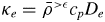 $\kappa _e = {\bar {\rho }^{{>}\epsilon }} c_p D_e$, where the eddy-diffusivity coefficient provided by the AMD model, namely
 \begin{equation} D_e = C \frac{\max\left(-\dfrac{\hat \partial \tilde{u}_i}{\partial \xi_k}\dfrac{\hat \partial \tilde{T}}{\partial \xi_k}\dfrac{\partial \tilde{T}}{\partial x_i},0\right)}{\dfrac{\partial \tilde{T}}{\partial x_l}\dfrac{\partial \tilde{T}}{\partial x_l}} , \end{equation}
involves scaled gradients of both velocity and temperature fields. It is worth noting that, to prevent numerical instabilities, the above closure modelling procedure does not admit backscatter effects, being limited to positive values of  $\nu _e$ and
 $\kappa _e$, through the use of the clipping procedure. Furthermore, the model constant
 $C$ is demonstrated to depend on the order of accuracy of the discretization method (Rozema et al. Reference Rozema, Bae, Moin and Verstappen2015). For the central fourth-order finite-difference method used in this study, the model constant is set to
 $C=0.212$, in accordance with the original formulation.
Remarkably, as the present SGS model algorithm does not require any test-level filtering, spatio-temporal averaging or solving additional transport equations, it has got inherent cost benefits over models involving dynamic procedures (e.g. Moin et al. Reference Moin, Squires, Cabot and Lee1991; De Stefano et al. Reference De Stefano, Vasilyev and Goldstein2008). The proposed closure modelling approach provides a built-in localized dynamic estimation of the SGS terms in the governing equations that takes full advantage of the adaptivity of the WA-LES solution. Complex turbulent flows can be simulated without introducing any spatial average, as is usually done in order to stabilize the numerical solution (Vreman et al. Reference Vreman, Geurts and Kuerten1997). Furthermore, the AMD model exhibits attractive convergence properties, since the actual importance of the modelled terms is implicitly coupled to the thresholding level, while automatically vanishing in well-resolved flow regions. Finally, the model coefficients (3.28) and (3.29) involve only algebraic reductions of velocity and temperature gradients, respectively, and are simply extendable to curvilinear meshes.
4. Numerical experiments
The present study examines the application of the proposed compressible LES method for wall-bounded attached turbulent flows, a hereto-unexplored context for wavelet-based computational modelling approaches. The numerical experiments implement a well-established benchmark configuration, that is, the turbulent supersonic isothermal-wall plane channel flow.
4.1. Case settings
Isothermal conditions are imposed at the channel walls, while periodic boundary conditions are applied along the two homogeneous directions. Scaled by the channel half-height  $H$, the size of the physical domain is
 $4{\rm \pi} H \times 2 H \times 4{\rm \pi} H / 3$, where the spatial coordinates
 $(x_1,x_2,x_3)$ are aligned with the streamwise, wall-normal and spanwise directions, respectively. The results of the pioneering works by Coleman and coauthors (Coleman, Kim & Moser Reference Coleman, Kim and Moser1995; Huang et al. Reference Huang, Coleman and Bradshaw1995) are usually considered as the reference solution for both DNS (Lechner, Sesterhenn & Friedrich Reference Lechner, Sesterhenn and Friedrich2001; Morinishi, Tamano & Nakabayashi Reference Morinishi, Tamano and Nakabayashi2004; Modesti & Pirozzoli Reference Modesti and Pirozzoli2016) and LES (Lenormand et al. Reference Lenormand, Sagaut and Ta Phuoc2000a; Brun etal. Reference Brun, Petrovan Boiarciuc, Haberkorn and Comte2008) studies.
In the following discussion, for clarity of notation, the resolved flow variables are denoted by using simple symbols. For example, the resolved density and temperature fields are denoted by  $\rho$ and
 $T$ (instead of
 ${\bar {\rho }^{{>}\epsilon }}$ and
 $\tilde T$). The bulk Reynolds and Mach numbers of the flow are
 ${Re} = \rho _m U_m H / \mu _w$ and
 ${Ma} = U_m/c_w$, where the mean bulk density and mass flux are defined as
 \begin{equation} \rho_m = \frac 1 {2H} \int_{-H}^{H} \bar \rho \, \textrm{d} x_2 \end{equation}
and
 \begin{equation} \rho_m U_m = \frac 1 {2H} \int_{-H}^{H} \overline{\rho u_1}\, \textrm{d} x_2, \end{equation}
respectively. In the above equations, the overbar is used to denote spatial averages in the homogeneous plane  $(x_1,x_3)$. The constant values
 $\mu _w$ and
 $c_w$ represent the molecular viscosity and the speed of sound evaluated at the wall temperature that is prescribed as
 $T_w = 293.15\ \textrm {K}$. Using air as the fluid, the molecular Prandtl number and the specific heat ratio are prescribed as
 ${Pr}=0.72$ and
 $\gamma =1.4$, respectively, while
 $R=287\ \text {J kg}^{-1}\,\text {K}^{-1}$ holds for the gas constant. The dependence of the dynamic viscosity on the temperature
 $\mu (T)$ is assumed to be given by Sutherland's law, which is here normalized as follows:
 \begin{equation} \frac{\mu}{\mu_w} = \frac{T_w + S}{T + S} \left( \frac{T}{T_w} \right)^{3/2}, \end{equation}
where  $S= 110.4\ \textrm {K}$ and
 $\mu _w = 1.81 \times 10^{-5}\ \text {kg m}^{-1}\,\text {s}^{-1}$. For the speed of sound, it is assumed that
 $c(T) = (\gamma R T)^{1/2}$. Unitary values are prescribed for the channel half-height and the mean bulk mass flux, which results in fixing
 $\mathcal {F}_0=1\ \text {kg m}^{-2}\,\text {s}^{-1}$ in (3.26). The simulations are analysed in terms of wall parameters, which are the friction Reynolds number
 ${Re}_{\tau } = \rho _w u_{\tau } H/\mu _w$, the friction Mach number
 ${Ma}_{\tau } = u_{\tau }/c_w$, and the heat flux coefficient
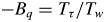 $-B_q = T_{\tau }/T_w$. The friction velocity and temperature are defined by
 $u_{\tau }=(\tau _w/\rho _w)^{1/2}$ and
 $T_{\tau } = -q_w / (\rho _w c_p u_{\tau })$, respectively, where
 $\rho _w$,
 $\tau _w$ and
 $q_w$ represent the wall-averaged values of resolved density, wall shear stress and wall heat flux.
In this work, the DNS results of Coleman and coauthors, which are available at the web page https://turbmodels.larc.nasa.gov/Other_DNS_Data/supersonic-channel.html, are used as reference data. The numerical experiments are conducted for both test cases considered there, namely at  ${Re} = 3000$ and
 ${Ma} = 1.5$ (case I) and
 ${Re} = 4880$ and
 ${Ma} = 3$ (case II). This allows for a detailed comparison of mean flow variables and turbulent stress profiles across the channel. However, since the corresponding mesh resolution can be considered marginal nowadays, the more recent DNS results of Modesti & Pirozzoli (Reference Modesti and Pirozzoli2016) are also considered for comparison. Furthermore, the results provided by Brun et al. (Reference Brun, Petrovan Boiarciuc, Haberkorn and Comte2008), which were obtained for the same computational domain, are employed as reference non-adaptive LES data.
4.2. Simulation settings
The solution of the WA-LES governing equations (3.10), (3.24) and (3.25), including the closure terms, is attained by employing the fourth-order A-AWC method, supplied with the linearized Crank–Nicolson split-step time integration method with adaptive time stepping, and the parallel version of the wavelet-based solver (Nejadmalayeri et al. Reference Nejadmalayeri, Vezolainen, Brown-Dymkoski and Vasilyev2015). The discretization of the three-dimensional computational domain is accomplished, for the test case I, by making use of seven nested wavelet collocation grids, which corresponds to set  $n=3$ and
 $J=7$ in the WTF definition (2.2), with the coarsest and the finest grid consisting of
 $12 \times 9 \times 8$ and
 $768 \times 513 \times 512$ wavelets, respectively. As is permitted by A-AWC, the corresponding meshes in the physical domain are stretched in the wall-normal direction, according to a hyperbolic tangent distribution. For the finest grid, the minimum mesh spacing in the wall-normal direction, which is set to
 ${\rm \Delta} x_{2,w} / H = 5.7 \times 10^{-4}$ at the walls, practically corresponds to that used by Coleman et al. (Reference Coleman, Kim and Moser1995). For the test case II, eight levels of resolution are prescribed (
 $J=8$), with the maximum resolution corresponding to
 $1536 \times 1025 \times 1024$ wavelets and
 ${\rm \Delta} x_{2,w} / H = 2.9 \times 10^{-4}$. The numerical simulations, where the first three levels of resolution (
 $1 \le j \le 3$) are kept non-adaptive, are conducted by using the balanced variables and the temperature field as sensors for the WTF procedure, in order to capture both kinematically and thermodynamically significant phenomena. It is worth noting that, due to the dynamic grid adaptation process, the above nominal maximum resolutions are potentially but not necessarily involved in the real computations. Moreover, only a low fraction of the total number of wavelets belonging to each wavelet collocation grid is actually employed.
The numerical simulation is initialized with a parabolic streamwise velocity profile, along with constant density and temperature, throughout the flow domain. Following Butler & Farrell (Reference Butler and Farrell1992), optimal perturbations are superimposed upon the initial velocity field to hasten the transition to fully developed turbulence. The low initial wavelet threshold of  $1 \times 10^{-3}$ is used for the first several flow-through times, in order to limit the damping effects of the wavelet filter on low-amplitude instabilities and permitting them to grow freely. The subsequent increased computational cost is mitigated by the fact that the early-time solution is relatively smooth. After this initial phase, the threshold is raised up to the prescribed value for the actual WA-LES calculation, which is
 $\epsilon =2.5 \times 10^{-2}$ for the test case I. As demonstrated in past studies, the choice of the uniform level of thresholding is very important, especially when no explicit filtering operation is performed and the pure built-in filtering effect of the wavelet-based grid adaptation is exploited (De Stefano & Vasilyev Reference De Stefano and Vasilyev2013). Therefore, the above parameter is selected as a fair compromise to ensure the necessary numerical accuracy, while keeping the computational cost acceptable. However, the detailed discussion of how the WTF level affects the WA-LES solution is included in § 4.4.
4.3. Results and discussion
In order to examine the resolved turbulent flow field at a given time instant, the adapted grid for the WA-LES solution at  ${Re} = 3000$ and
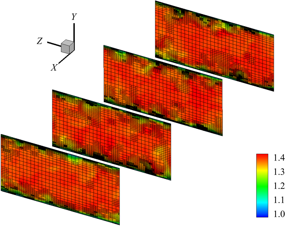
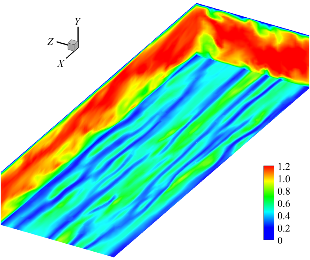
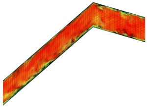
 ${Ma} = 1.5$ is illustrated in figure 1, together with the temperature contours, for four different cross-sections along the channel that are equispaced in the streamwise direction. The mesh stretching in the wall-normal direction is apparent, as well as the mesh refinement around localized flow structures. The corresponding contours of the streamwise velocity component at three different channel sections aligned with the coordinate planes are illustrated in figure 2, where the flow field is shown for
 $x_2/H \ge -0.96$. The elongated streak-like flow structures in the wall region are apparent. For the solution at
 ${Re} = 4880$ and
 ${Ma} = 3$, which is obtained by using
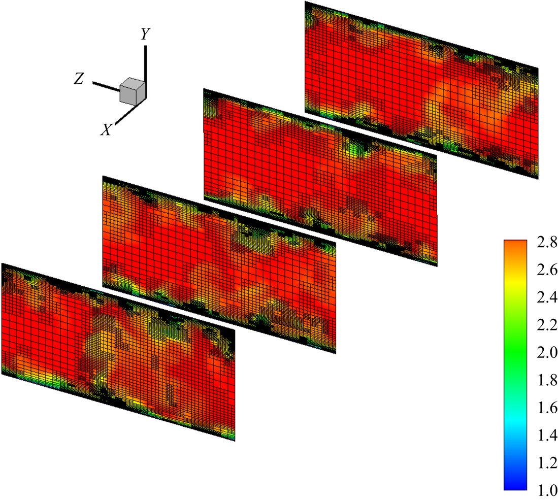
 $\epsilon =1.5 \times 10^{-2}$, an example of an instantaneous adapted grid, together with the associated temperature contours, is shown in figure 3.
Adaptive spatial grid and temperature contours, at a given time instant, for the simulation with  ${Ma} = 1.5$ (case I), for four different equispaced cross-sections of the channel (
 $X,Y,Z$ represent the streamwise, wall-normal and spanwise directions).

Streamwise velocity contours, at a given time instant, for the simulation with  ${Ma} = 1.5$ (case I), for the channel sections at
 $x_1/H=0$,
 $x_2/H=-0.96$ and
 $x_3/H=4{\rm \pi} /3$ (
 $X,Y, Z$ represent the streamwise, wall-normal and spanwise directions).

Adaptive spatial grid and temperature contours, at a given time instant, for the simulation with  ${Ma} = 3$ (case II), for four different equispaced cross-sections of the channel (
 $X,Y,Z$ represent the streamwise, wall-normal and spanwise directions).

As is typical for WTF-based simulations, only a subset of the available collocation points is actually involved in the calculations. The grid compression is defined, level by level, as the percentage of discarded wavelets with respect to the nominally available ones. The time-averaged grid compression data are reported in tables 1 and 2, for the test cases I and II, respectively. The maximum level of resolution is actually not involved in the computations. In fact, the finest grid that is employed corresponds to the sixth (seventh) level for the test case I (II), which suffices to fully support the resolved fields. However, prescribing  $J=7$ (
 $J=8$) makes it possible to empirically demonstrate the actual resolution of the ongoing simulation. The high grid compression that is achieved in the present compressible flow cases is comparable to that found in past incompressible WA-LES studies (e.g. De Stefano & Vasilyev Reference De Stefano and Vasilyev2010, Reference De Stefano and Vasilyev2012, Reference De Stefano and Vasilyev2014).
Time-averaged grid compression and mesh spacings for different levels of resolution, for the simulation with  ${Ma} = 1.5$ (case I).

Time-averaged grid compression and mesh spacings for different levels of resolution, at a given time instant, for the simulation with  ${Ma} = 3$ (case II).

The mesh spacings along each spatial direction are also reported in tables 1 and 2. They are expressed in viscous wall units, namely  ${\rm \Delta} x_i^+ = Re_{\tau } {\rm \Delta} x_i/H$, given the time-averaged friction Reynolds number that is achieved in the simulations.
It is worth noting that, in this study, finer spatial resolution is permitted in the homogeneous directions with respect to reference DNS, where a different higher-order numerical approach using a Fourier–Legendre spectral discretization was utilized (Coleman et al. Reference Coleman, Kim and Moser1995). The lower aspect ratio of the computational cells is used because it has been empirically found to lead to retaining fewer grid points in the overall adaptation process. However, the increased resolution in the streamwise and spanwise directions does not affect the time-step size restriction, which is practically imposed by the acoustic stiffness in the wall-normal direction. Moreover, the strong grid compression that is practically achieved in the simulations makes the WA-LES approach very efficient. When making a comparison with non-adaptive LES, the increased per-point computational cost of the wavelet-based adaptive solution, which is approximately three times heavier, must be taken into account. In order to obtain a fair correlation, the cost is evaluated at the finest-but-one level of resolution, namely at the fifth (sixth) level for the test case I (II). Based on the time-averaged grid compression reported in table 1 (table 2), the cost of a corresponding non-adaptive calculation would be  $40\,\%$ (seven times) higher. Predictably, the WA-LES approach becomes more and more effective with increasing Reynolds number. Further research, similar to what was performed in Kevlahan, Alam & Vasilyev (Reference Kevlahan, Alam and Vasilyev2007) and Nejadmalayeri, Vezolainen & Vasilyev (Reference Nejadmalayeri, Vezolainen and Vasilyev2013) for homogeneous isotropic turbulence, will be required to fully characterize the Reynolds-number scaling of the proposed methodology for high-speed compressible flows.
The flow statistics are computed from the adaptive grids by means of fourth-order wavelet interpolation onto regular non-adaptive sampling grids, at the finest level of resolution that is really employed in the simulations. As is appropriate for the present plane channel flow, once fully developed turbulent flow conditions are achieved, the Reynolds-averaged fields are computed by employing a long-time averaging procedure, conducted over 12 flow-through times, along with spatial averaging in the streamwise and spanwise homogeneous directions. The mean flow and turbulence statistics are evaluated in terms of Reynolds-averaged variables and corresponding fluctuations. In the following discussion, mean flow quantities are denoted by angular brackets. The profiles of mean temperature  $\langle T \rangle$, normalized with
 $T_w$, and mean density
 $\langle \rho \rangle$, normalized with
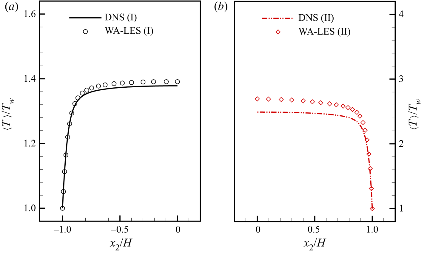
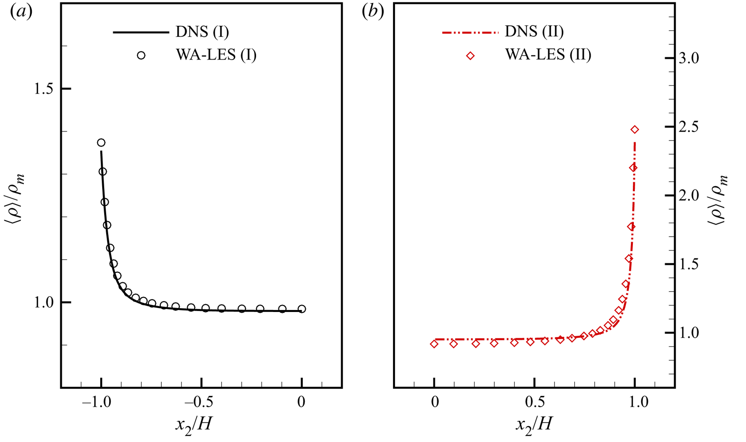
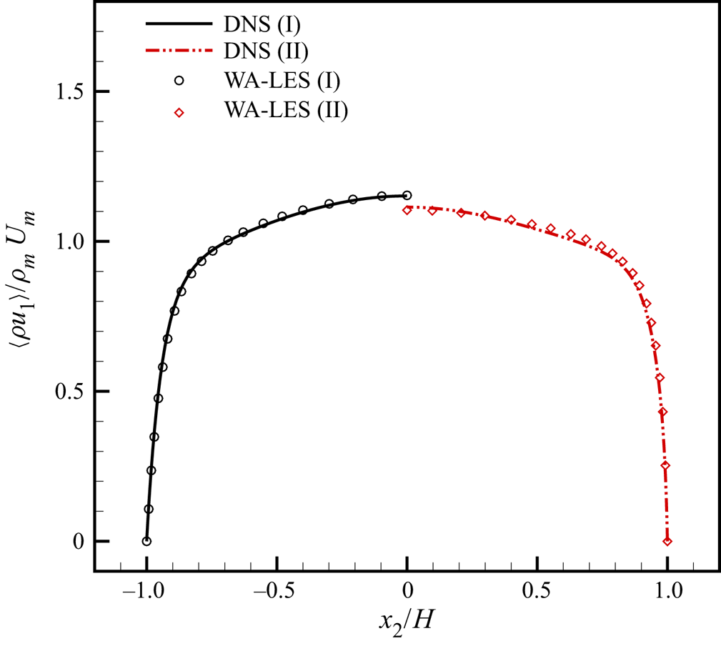
 $\rho _m$, are reported in figures 4 and 5, respectively. Also, the mean streamwise momentum (per unit volume)
 $\langle \rho u_1 \rangle$, normalized with the bulk mass flux
 $\rho _m U_m$, is shown in figure 6. Here, as well as in the following figures, the profiles across the half-channel height are shown, for both test cases, by averaging the corresponding data on the two sides of the channel, compared to the reference DNS results by Coleman et al. (Reference Coleman, Kim and Moser1995). Owing to the prescribed condition of isothermal walls, the fluid is cooled due to the heat transfer by convection at the walls, where the maximum gradients of mean temperature and density occur.
Mean temperature profiles: present WA-LES compared to reference DNS (Coleman et al. Reference Coleman, Kim and Moser1995), for the simulations with (a)  ${Ma}=1.5$ (case I) and (b)
 ${Ma}=3$ (case II).

Mean density profiles: present WA-LES compared to reference DNS (Coleman etal. Reference Coleman, Kim and Moser1995), for the simulations with (a)  ${Ma}=1.5$ (case I) and (b)
 ${Ma}=3$ (case II).

Mean streamwise momentum profiles: present WA-LES compared to reference DNS (Coleman et al. Reference Coleman, Kim and Moser1995), for the simulations with  ${Ma}=1.5$ (case I) and
 ${Ma}=3$ (case II).

As is apparent, the temperature in the centre of the channel and the wall density increase with the Mach number. The mean temperature in the mid-section of the channel is slightly overestimated, with the discrepancy increasing with the Mach number. This is consistent with reference LES data, as demonstrated in tables 3 and 4, where some mean flow results are shown for the two different configurations. In these tables, instead of reporting the numerical resolution corresponding to the finest grid that is employed in the WA-LES calculations, the mesh spacings corresponding to a reference, say equivalent, non-adaptive grid are shown. The equivalent grid is defined by not altering the relative number of points along the three spatial directions, while approximately matching the overall number of retained grid points. The latter is evaluated based on the averaged grid compression values previously reported, which are  $96.2\,\%$ and
 $99.4\,\%$, for the test cases I and II, respectively. This way, a more meaningful comparison between present WA-LES and reference non-adaptive simulations is achieved when examining the resolution in the homogeneous directions. Unfortunately, this is not true for the wall-normal non-homogeneous direction, for which it is more appropriate to look at the minimum mesh spacings associated with the finest collocation grids, which are shown in parentheses. For the test case I, the wall parameters that are provided by the present numerical experiment are underestimated with respect to DNS, consistently with the level of fidelity introduced by the WTF procedure. The discrepancy is found to be lower when considering the more refined DNS results of Modesti & Pirozzoli (Reference Modesti and Pirozzoli2016). For the test case II, the friction Reynolds number is slightly overestimated with respect to DNS, whereas the friction Mach number and the heat flux coefficient are slightly underestimated. However, the comparison with reference LES gives acceptable results.
Numerical resolution and mean flow results at  ${Ma}=1.5$ and
 ${Re}=3000$ (case I): present WA-LES compared to reference DNS by Coleman et al. (Reference Coleman, Kim and Moser1995) (1), DNS by Modesti & Pirozzoli (Reference Modesti and Pirozzoli2016) (2), and LES by Brun et al. (Reference Brun, Petrovan Boiarciuc, Haberkorn and Comte2008) (3). For WA-LES, the resolution corresponding to an equivalent non-adaptive grid is shown.

Numerical resolution and mean flow results at  ${Ma}=3$ and
 ${Re}=4880$ (case II): present WA-LES compared to reference DNS by Coleman et al. (Reference Coleman, Kim and Moser1995) (1), DNS by Modesti & Pirozzoli (Reference Modesti and Pirozzoli2016) (2), and LES by Brun et al. (Reference Brun, Petrovan Boiarciuc, Haberkorn and Comte2008) (3). For WA-LES, the resolution corresponding to an equivalent non-adaptive grid is shown.

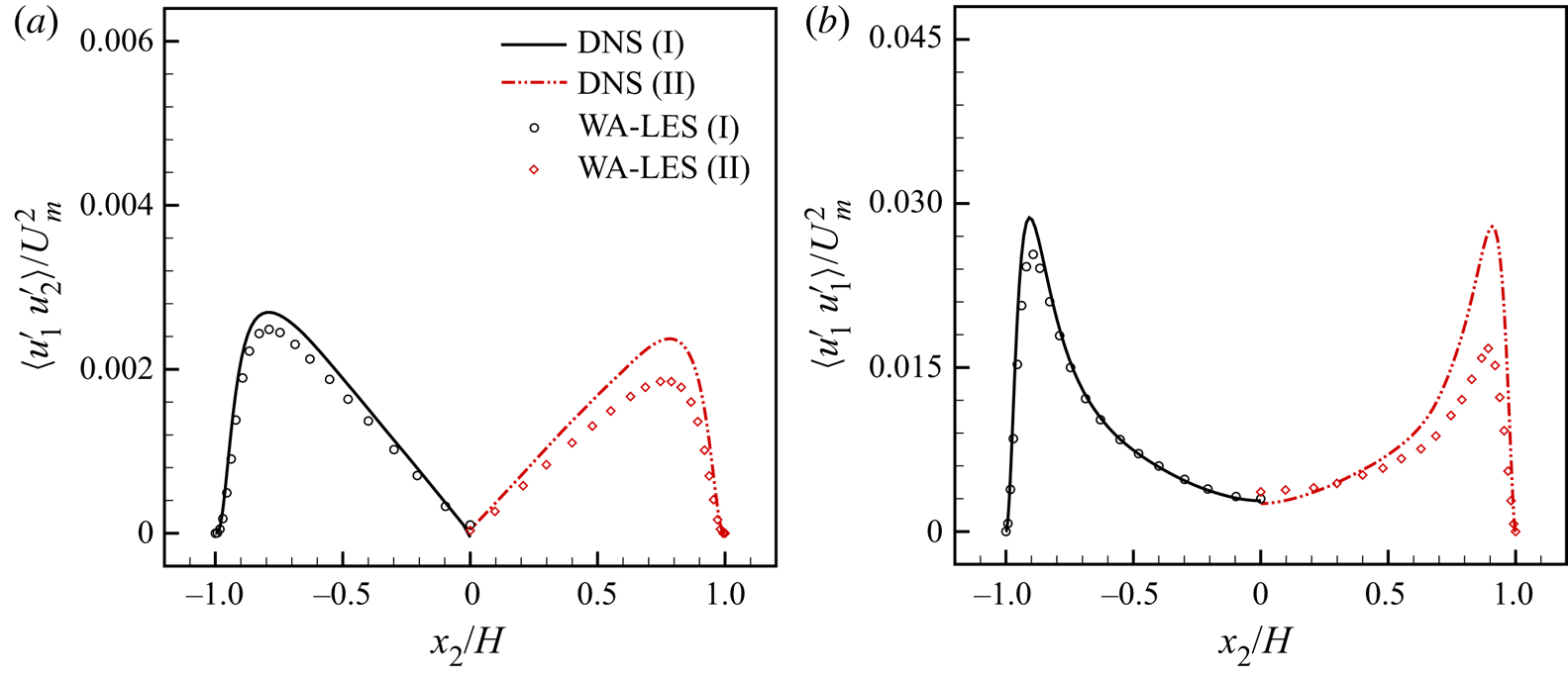
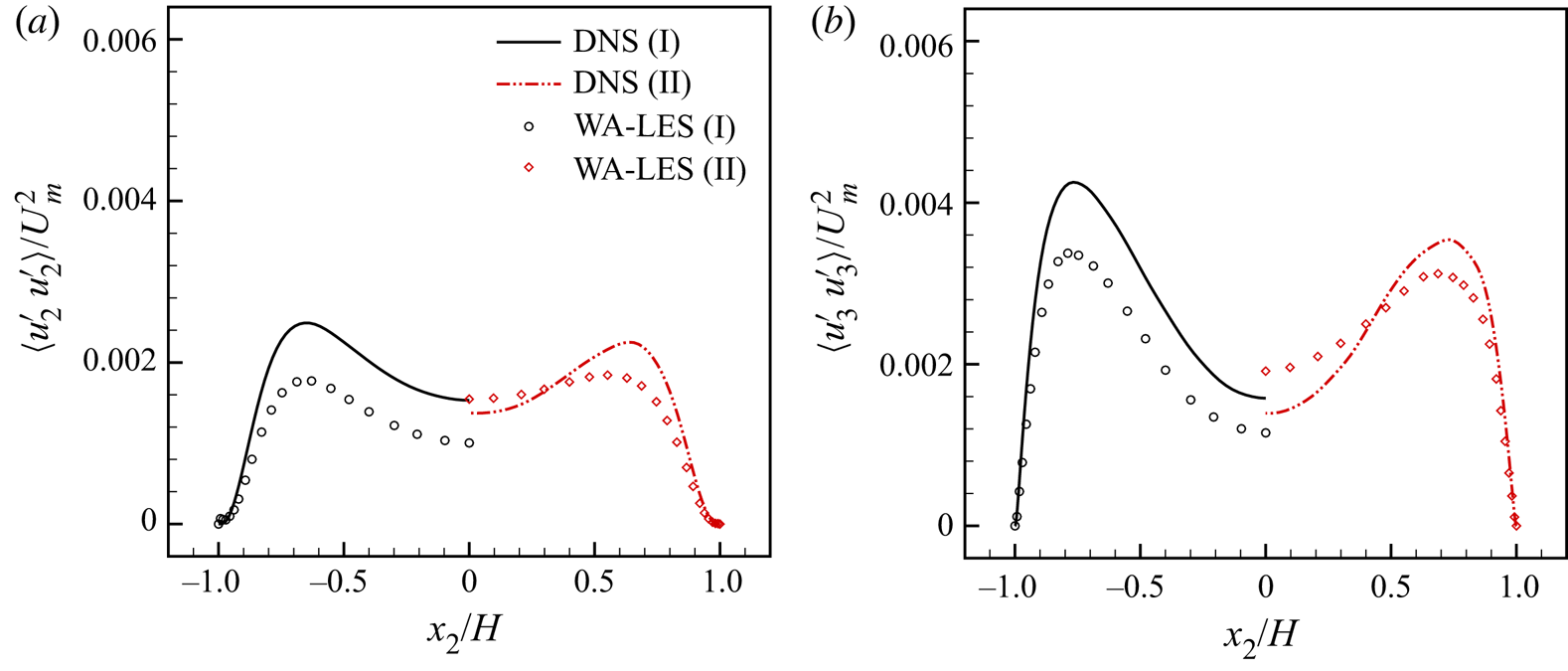
The WA-LES solutions are further analysed in terms of resolved turbulent stresses. To make a direct comparison with DNS data by Coleman et al. (Reference Coleman, Kim and Moser1995), the velocity fluctuation covariances, namely  $\langle u_i^{\prime } u_j^{\prime } \rangle$, with the apex denoting Reynolds fluctuations,
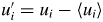 $u_i^{\prime } = u_i -\langle u_i \rangle$, are considered. The shear stress
 $\langle u_1^{\prime } u_2^{\prime } \rangle$ and the normal stress in the streamwise direction
 $\langle u_1^{\prime } u_1^{\prime } \rangle$ are reported in figure 7, while the normal stresses in the wall-normal and spanwise directions,
 $\langle u_2^{\prime } u_2^{\prime } \rangle$ and
 $\langle u_3^{\prime } u_3^{\prime } \rangle$, are drawn in figure 8, normalized with
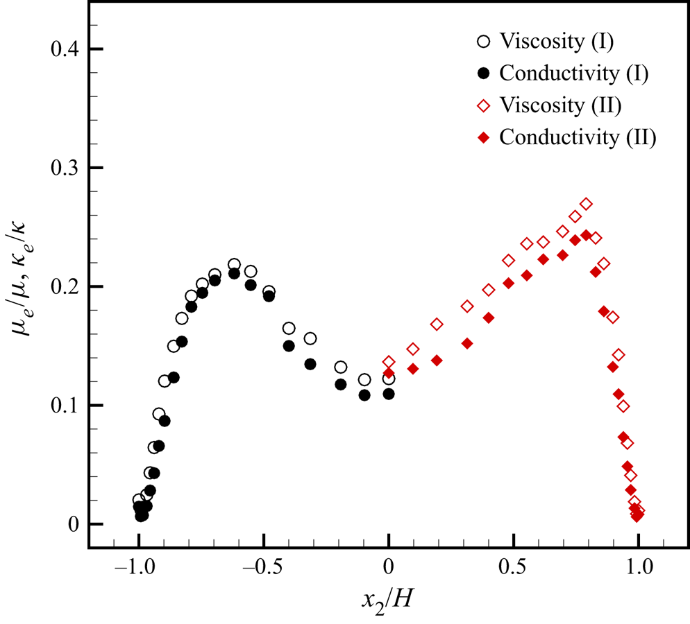
 $U_m^2$. The resolved turbulent stresses show good agreement with the benchmark results, in particular the location of the peaks corresponding to the turbulence-producing regions close to the walls is predicted well. However, the stress magnitudes computed from the WA-LES calculations are generally lower than found in DNS, because the energy content of the discarded wavelet modes is non-negligible and the SGS contribution to the Reynolds stresses is responsible for the differences. By inspection of figure 8, for the simulation with higher Mach number, the normal stresses in the transverse plane are somewhat overestimated in the centre of the channel. The modelled dissipation represents a substantial fraction of the total dissipation, as demonstrated in figure 9, where the plane-averaged ratios of turbulent eddy viscosity and eddy conductivity to corresponding molecular values,
 $\mu _e/\mu$ and
 $\kappa _e/\kappa$, are reported at a given time instant. The present values of these ratios are perfectly consistent with previous findings for incompressible WA-LES (e.g. De Stefano & Vasilyev Reference De Stefano and Vasilyev2012). It is worth stressing that the modelled SGS terms provided by the AMD approach automatically converge to zero at the walls, where the eddy viscosity and the eddy conductivity vanish, without needing the use of any additional damping functions.
Turbulent shear stress (a) and streamwise normal stress (b) profiles: present WA-LES compared to reference DNS (Coleman et al. Reference Coleman, Kim and Moser1995), for the simulations with  ${Ma}=1.5$ (case I) and
 ${Ma}=3$ (case II).

Turbulent wall-normal (a) and spanwise (b) normal stress profiles: present WA-LES compared to reference DNS (Coleman et al. Reference Coleman, Kim and Moser1995), for the simulations with  ${Ma}=1.5$ (case I) and
 ${Ma}=3$ (case II).

Plane-averaged ratios of eddy viscosity to molecular viscosity and eddy conductivity to molecular conductivity, for the simulations with  ${Ma}=1.5$ (case I) and
 ${Ma}=3$ (case II).

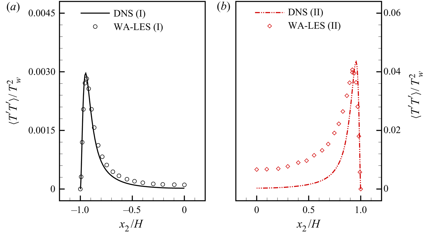
To ascertain the ability of the novel WA-LES approach to adequately capture compressibility effects, while simulating turbulent fluctuations in the thermodynamic state variables, the profiles of mean-square temperature fluctuations  $\langle T^{\prime } T^{\prime } \rangle$, normalized with
 $T^2_w$, are examined in figure 10. The comparison with reference DNS is consistent with previous analysis for the turbulent stresses. For the test case I, the solution aligns very well with the benchmark data, practically capturing the peak value, whereas, for the test case II, the temperature fluctuations are overestimated in the core of the channel. The present results are comparable to classical non-adaptive LES data. For instance, by looking at the streamwise velocity and temperature variances for the test case I, the corresponding DNS peak values are presently missed by
 $-9\,\%$ and
 $-4\,\%$, respectively, while discrepancies in the range
 $-7\,\%$ to
 $+9\,\%$ for the streamwise velocity and
 $-9\,\%$ to
 $0\,\%$ for the temperature are provided in Lenormand et al. (Reference Lenormand, Sagaut, Ta Phuoc and Comte2000b).
Mean-square temperature fluctuation profiles: present WA-LES compared to reference DNS (Coleman et al. Reference Coleman, Kim and Moser1995), for the simulations with (a)  ${Ma}=1.5$ (case I) and (b)
 ${Ma}=3$ (case II).

The accuracy of the resolved turbulent fluctuations in the wall region demonstrates an important feature of the present compressible WA-LES approach. Owing to the automatic adaptation process, close to the walls, the presence of high gradients in the mean flow-field variables, along with significant turbulent fluctuations, leads to the use of finer grids. This effect also contributes to the retention of energy for the high-wavenumber modes and the commensurately increased local resolution with respect to classical low-pass filter-based non-adaptive LES methods. In contrast, in the central region of the channel, due to the slowly spatially varying mean flow and less significant turbulence, coarser grids are employed in the calculation. Therefore, the disparate flow conditions result in different numerical resolution that affects the AMD modelling procedure, particularly at higher Mach number. The issue could be addressed by using a more sophisticated dynamic modelling procedure, the implementation of which is deferred to future work.
4.4. Level of thresholding
In order to practically explore how the WTF level affects the WA-LES solution, some additional simulations are performed by varying this parameter. Specifically, four calculations, with  $\epsilon = 7.5 \times 10^{-2}$,
 $5 \times 10^{-2}$,
 $2.5 \times 10^{-2}$ and
 $1.5 \times 10^{-2}$, are compared for the benchmark case I. The statistics for the different computations are accumulated for the same period of time, corresponding to 12 flow-through times, except for the simulation with the lowest threshold. In fact, due to the much lower grid compression and the corresponding high computational cost, being not considered representative of the WA-LES regime, the latter solution is not carried out for the time necessary to achieve fully converged statistics.
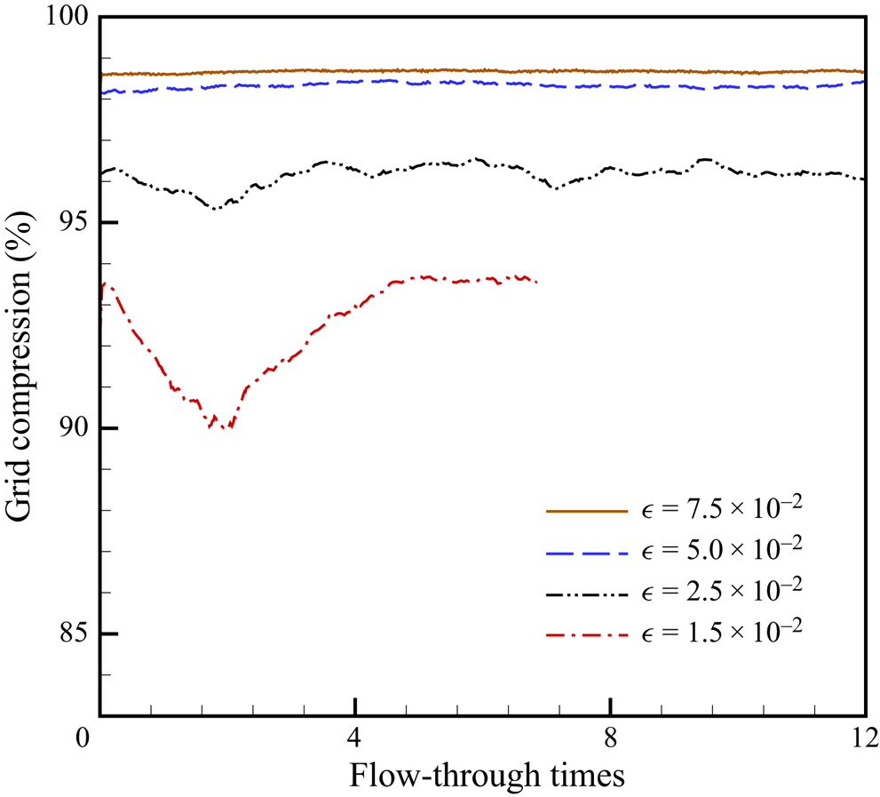
As demonstrated in figure 11, where the time history of the grid compression for the different solutions is reported, as expected the numerical resolution increases with decreasing threshold. In table 5, the time-averaged grid compression that is obtained by the different calculations is reported along with some mean flow results. The seventh level of resolution is employed only by the calculation with the lowest threshold. However, for a meaningful comparison, the reported compression is evaluated with respect to the sixth level of resolution also in the latter case. Furthermore, the choice of  $J=8$ as nominal maximum level of resolution in the wavelet decomposition (2.2) is empirically verified not to affect the calculations, since the eighth grid level is actually not involved in the simulations, regardless of the wavelet threshold that is prescribed.
Time history of the grid compression for different thresholding levels.

Time-averaged grid compression and mean flow results for different thresholding levels.

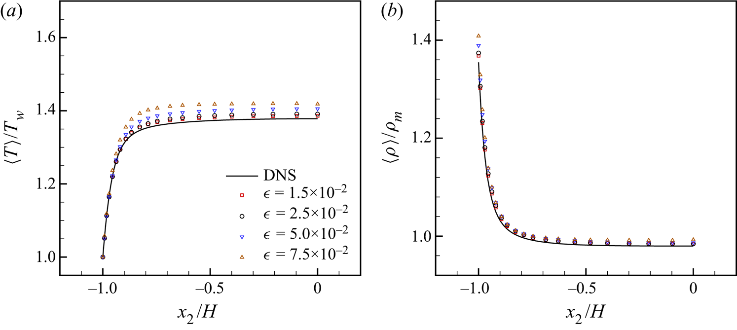
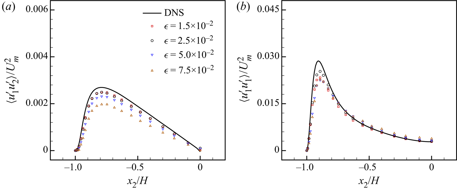
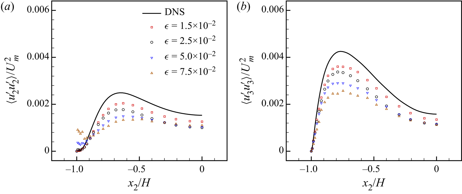
The resolved mean flow is found to be influenced by the thresholding level, which directly controls the numerical accuracy of the solution. For decreasing threshold, the profiles of mean flow quantities approach the reference DNS, as illustrated in figure 12 for the temperature and the density fields. As to the resolved turbulent stresses, they markedly depend on the WTF parameter, which also controls the turbulence resolution of the WA-LES method. The lower the threshold is, the better the turbulent fluctuations are approximated. This is demonstrated in figures 13 and 14, where the profiles of shear and normal stresses for the different levels of thresholding are depicted. The small inaccuracy of the streamwise normal stress for the lowest threshold is to be attributed to the fact that the related time average would take longer to fully converge.
Mean temperature (a) and mean density (b) profiles for WA-LES with different thresholding levels, compared to reference DNS (Coleman et al. Reference Coleman, Kim and Moser1995).

Turbulent shear stress (a) and streamwise normal stress (b) profiles for WA-LES with different thresholding levels, compared to reference DNS (Coleman et al. Reference Coleman, Kim and Moser1995).

Turbulent wall-normal (a) and spanwise (b) normal stress profiles for WA-LES with different thresholding levels, compared to reference DNS (Coleman et al. Reference Coleman, Kim and Moser1995).

The results of this sensitivity study confirm that the present wavelet-based computational modelling procedure tends towards the direct solution of the unfiltered equations for decreasing threshold, which substantiates the theoretical analysis presented in § 3.2. Practically, the wavelet filter width decreases with the thresholding level and the resolved wavelet-filtered turbulent fields approach the unfiltered ones.
5. Conclusions
The wavelet-based adaptive large-eddy simulation (WA-LES) method for computational turbulence modelling has been originally extended to the compressible flow regime and successfully tested for fully developed attached turbulent flow. Numerical experiments have been conducted for supersonic turbulent channel flow with isothermal walls at different Reynolds and Mach numbers. The present wall-bounded compressible flow configuration represents a hereto-unexplored problem for wavelet-based modelling procedures. The anisotropic minimum-dissipation (AMD) modelling approach has been developed to close the nonlinear terms that arise from wavelet filtering of the compressible Navier–Stokes equations. The employed eddy-viscosity and eddy-conductivity models have shown favourable convergence properties, as the modelled terms automatically vanish for well-resolved flow regions.
Of particular note for the present high-speed flow regime, thermodynamic quantities have been reasonably captured through the compressible WA-LES approach. The turbulent fluctuations have been almost universally underpredicted with respect to DNS of the same flow, which is consistent with the level of turbulence resolution that is intrinsically imposed by the wavelet threshold filtering procedure. As demonstrated by means of a sensitivity analysis, for decreasing levels of thresholding, the resolved wavelet-filtered turbulent fields approach the unfiltered ones, as is expected for implicit filtering LES methods.
Also based on the comparison with classical non-adaptive LES data, the present results demonstrate both the feasibility and the effectiveness of the novel wavelet-based computational modelling approach. The good performance of the WA-LES method supplied with the AMD model makes it a viable alternative to the traditional LES approaches in the simulation of compressible wall-bounded attached turbulent flows.
Acknowledgements
This work has been partially supported by the Russian Science Foundation (Project 16-11-10350). This support is gratefully acknowledged. The authors also acknowledge the CINECA award under the ISCRA initiative (Project HP10B67O33) for the availability of high-performance computing resources.
Declaration of interests
The authors report no conflict of interest.