

Formal political theory has provided powerful analytical grounding for the study of elections and voting. Yet it is quite difficult to find situations that provide empirical settings in which even relatively simple formal theory can be tested in a fairly straightforward way. In this article, we analyze a set of election data that permit simple tests of “rational” voting and agenda setting. We put rational in quotation marks because we eschew venturing into an extensive discussion of what constitutes rationality. We are more narrowly concerned with testing whether behavior is consistent with voters applying the game-theoretic concept of iterated weak dominance. Voters are presumed to move in a one-shot subgame that follows either one or two proposals made by the agenda setter. The agenda setter is assumed to be a budget-maximizer who optimizes presuming that iterated weak dominance is used in the subgame.
Our empirical context is school district operating budget referenda in the state of Oregon. For many years, such referenda were an instance of democracy in about half of all US states (Berkman and Plutzer Reference Berkman and Plutzer2005). Oregon held these elections for many years until the 1990s, and served as the quintessential case that motivated the Romer-Rosenthal (Reference Romer and Rosenthal1978, Reference Romer and Rosenthal1979, Reference Romer and Rosenthal1982a, Reference Romer and Rosenthal1982b) model of agenda control by a budget-maximizing bureaucrat—in this context, the local school board.
In this article, we exploit an institutional feature of Oregon school elections that was present in the 1980–81 through 1983–84 school years.Footnote 1 In some cases voters were asked to vote simultaneously on two expenditure amounts that together comprised the locally funded portion of the school budget. We use data from these referenda to test whether aggregate election results are consistent with “rational” voter behavior under the assumption of single-peaked preferences, and agenda-setting behavior on the part of school district boards.
Much research in political science explores the situation in which voters make a simple binary choice. Rationality, in this instance, is simply voting for the preferred outcome. The “game” between voters is uninteresting. An extensive literature analyzes situations in which voters make a single choice but have multiple alternatives. In such contexts, modeling the voter game focuses on what voters do when they are pivotal to the outcome. Voters are strategic if, for example, they accept the cost of voting only when the election is close to a tie, or when they vote for their second-most-preferred outcome when their preferred outcome is unlikely to win.Footnote 2 In this article, we also examine the actions of pivotal voters when voters have two choices. Often, however, as in the literature on split-ticket voting, testing rationality in such instances becomes complicated due to both institutional complexities and data limitations, as in Mebane (Reference Mebane2000). By contrast, we develop a prediction that has a straightforward, direct test.
The 1980–83 Oregon data also allow for a new test of agenda-setting behavior. In the first two years of this period, school boards were required to split budget requests above a fixed amount into two expenditure proposals. In the last two years, boards could opt for a single expenditure proposal. In all four years, the alternative to a failed budget proposal was a fixed “reversion” amount that was typically much lower than the budget proposed by the school board. We make the strong assumption that the agenda setter is a budget maximizer (Niskanen Reference Niskanen1971; Romer and Rosenthal Reference Romer and Rosenthal1978, Reference Romer and Rosenthal1979) who will propose the highest budget that the electorate weakly prefers to the reversion amount. We show that, when given the choice, a budget-maximizing agenda setter should always make a single proposal rather than two separate proposals. We test this prediction by examining whether referenda were shifted to single proposals in the later period when the single-proposal option was available.
The election data also disclose an interesting regularity in the number of people who cast votes on the two expenditure levels. We simply present the regularity, and briefly discuss its interpretation in light of the voter information models developed by Feddersen and Pesendorfer (Reference Feddersen and Pesendorfer1997, Reference Feddersen and Pesendorfer1999) and the non-voting from indifference model of Hinich and Ordeshook (Reference Hinich and Ordeshook1969).
THEORY
We consider the following expenditure referendum. Voters are presented with a choice between a reversion level of spending Q and a higher level A. At the agenda setter’s discretion, there may also be a separate additional amount B to be voted on at the same time. Suppose both A and B proposals are present. If both A and B receive majorities, actual expenditure becomes Z≡A+B. If only A receives a majority, the actual expenditure is just A. If neither receives a majority, or if only B receives a majority,Footnote 3 the expenditure is Q. Thus the outcome set is {Q,A,Z}. Voter preferences are assumed to be single peaked. We also assume that all voters vote on both the A and B ballots (that is, no abstention). Finally, the reversion amount Q in future years is independent of current expenditure decisions. (This was the case in Oregon during the period of our data, though the rule changed in later years). Thus we can limit our consideration to a one-shot game.Footnote 4
Rational Voting
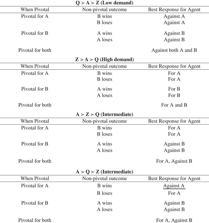
The pure strategy set of the voters can be described as {(For A, For B), (For A, Against B), (Against A, For B), (Against A, Against B)}. With single-peaked preferences, there are only four voter preference types (ignoring the knife-edge cases of indifference). Denoting the strict preference relation by ≻, these are Z ≻ A ≻ Q, A ≻ Z ≻ Q, A ≻ Q ≻ Z, and Q ≻ A ≻ Z. Any strategy is a best response if a voter is not pivotal. We can study whether each of these four types has weakly undominated voting strategies by exhaustively considering their best responses in situations when they are pivotal. A voter can be pivotal in one of three ways. First, the voter is decisive in both the A and B elections. Second, the voter is decisive only in the A election. Third, the voter pivots only in the B election. The analysis is summarized in Figure 1.
Best responses of the voter types (single-peaked preferences)

The situation for the low-demand type, Q ≻ A ≻ Z, is shown in the top panel in the figure. When a voter of this type is pivotal in both elections, a best response must include voting against A, since a vote against A leads to the most-preferred outcome of Q. When the voter is pivotal only in the B election, a best response must include voting against B. When the voter votes against B, Q results if A is losing, and A results if A is winning. Voting against both A and B is a best response if the voter is pivotal only in the A election. Consequently, voting ‘No’ in both elections is uniquely a weakly dominant strategy for the low-demand type.
The situation for the high-demand type, Z ≻ A ≻ Q, shown in the second panel in the figure, is simpler. When a voter of this type is pivotal in both elections, voting for A and for B is a unique best response. It can be readily checked that voting for A and B is a best response when the voter is pivotal in only one election. Hence, agents of the high-demand type have a weakly dominant strategy of voting ‘Yes’ in both elections.
The intermediate type, A ≻ Z ≻ Q, shown in the third panel in Figure 1, has a unique best response of voting for A and against B when the voter is pivotal in both elections. It can be readily checked that this strategy is also a best response when the voter is pivotal in only one election. Consequently, voting for A and against B is a weakly dominant strategy for this intermediate type.
Finally, the intermediate type A ≻ Q ≻ Z does not have a weakly dominant strategy. This type must also vote for A and against B when pivotal in both elections. This strategy is also a best response when a voter of this type is pivotal in only the B election. But it is not a best response when the voter is pivotal in only the A election. If, as shown in the bottom panel of Figure 1, B wins the B election, the voter must vote against A to obtain Q rather than the least-preferred outcome, Z.
The voter “knows,” however, that if the other three types use their weakly dominant strategies, A will receive at least as many votes from these types as does B. Moreover, the voter also “knows” that, for other A ≻ Q ≻ Z agents, voting for B is weakly dominated since a vote for B can only pivot to the least-preferred outcome, Z. Thus the type will never be in a position to be a pivotal voter for A but not for B. The only instance in which B wins is one in which the high-demand types are a majority, and if the high-demand types are pivotal for the B election they will also be pivotal for A. By iteration of weak dominance, therefore, voting for A and against B is a best response for the A ≻ Q ≻ Z type when the type is pivotal. When iterated weak dominance is applied, mixed strategies are also weakly dominated.
Note that in standard one-election situations with two alternatives, weak dominance is used to argue that all voters should vote sincerely. From the many Nash equilibria in a voting “game,” weak dominance selects the natural one based on sincere voting. In the two-election case we model here, there is one voter type (A ≻ Q ≻ Z) that does not have a weakly dominant strategy. We can, however, use iterated weak dominance to select a unique Nash equilibrium to the voting game.Footnote 5 Z ≻ A ≻ Q types are predicted to vote ‘Yes’ on both the A and B votes, while Q ≻ A ≻ Z types are predicted to vote ‘No’ on both. The two intermediate types are predicted to vote ‘Yes’ on A and ‘No’ on B. Note further that the strategies used by the voters do not depend on their knowledge of the number of voters of each type; that is, information about voter preferences can be complete or incomplete. In summary, we have the following proposition:
Proposition 1: If there is at least one voter of either type A ≻ Q ≻ Z or A ≻ Z ≻ Q, then the ‘No’ vote will be greater in the B election than in the A election. If there is no such voter, the ‘No’ vote in the B election will equal that in the A election.
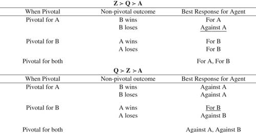
Proposition 1 does depend on the assumption of single-peaked preferences. In Figure 2 we show the situation for the two preference types that are not single peaked. The type Z ≻ Q ≻ A corresponds to individuals who prefer a high level of school expenditure but would rather not have public education if the schools are mediocre (for example, Stiglitz Reference Stiglitz1974). When a voter of this type is pivotal in both elections, the voter must vote for both A and B. If the voter is pivotal in only the A election and B is losing, the voter’s best response is to vote against A. So there is no weakly dominant best response. Moreover, the situation cannot be resolved by applying further iteration. When this voter votes against A, voting for B remains a best response, so A could get fewer votes than B. The situation is similar for the second preference type.
Best responses of a voter with non-single-peaked preference

We have stated Proposition 1 in terms of the aggregate vote totals. A stricter version would say that we should observe no individual who votes ‘Yes’ on the B ballot but ‘No’ on the A ballot. We do not have individual-level data, and can only test the aggregate implication of the proposition.
Agenda Setting
Suppose that the choices of the A and B amounts are made by a budget-maximizing agenda setter. In the institutional context of our data, which is covered in detail in the next section, in 1980 and 1981 the agenda setter was constrained by law to submit any expenditures less than a specified maximum to an A vote. Denote this maximum as Amax. Only if total proposed expenditures exceed Amax is a B vote required.Footnote 6 Expenditures up to Amax, as explained later, provide a tax subsidy for some voters.
Now suppose that a majority of the voters would approve expenditure at least equal to Amax. Relax the requirement that the setter must have a separate B vote on amounts greater than Amax, and assume that the agenda setter is permitted to make a single proposal C to the voters. Assume further that there is at least one intermediate-type voter who prefers Z (=Amax+B) to Q but prefers Amax to Z.
The next proposition states that the setter will prefer to make a bundled single proposal rather than separate A and B proposals. This proposition requires the setter to be completely informed about voter preferences.
Proposition 2: When given the option, the setter will make a single proposal C rather than separate proposals A and B.
Corollary. C >Amax +B if a majority of voters supports B.
Proposition 2 and the corollary follow from Romer and Rosenthal (Reference Romer and Rosenthal1978, 34, Proposition 2).Footnote 7 Let P(Q') be the setter’s budget-maximizing proposal when the reversion is Q'. Then for reversions Q1 and Q2 such that Q1 < Q2, P(Q1) >P(Q2) as long as a majority of voters prefers expenditures greater than Q2. In our context, the reversion under the single proposal C is Q, so C=P(Q). When two separate proposals are made, the second proposal is, in effect, the expenditure Z (=A + B) with reversion A (if A passes but B fails) and Q if A fails. Since A > Q, P(Q) > P(A), and so the setter cannot do worse with a single proposal than with the separate A and B proposals. If a majority prefer Amax + B to Amax then we must have P(Q) > P(Amax), that is, C > Amax + B. In a nutshell, in the ultimatum game between the setter and the voters, the setter’s threat is greater with one election than with two.
EMPIRICAL CONTEXT
For many years, Oregon’s school districts held financial elections. These elections were referenda in which school boards would propose a local budget that required approval by a majority of the voters. Through 1979, the budgets were simple all-or-nothing proposals to increase expenditure beyond a local reversion expenditure (Q) that was fixed exogenously. The reversion expenditure varied by district, and could be zero or a strictly positive amount. In some cases the reversion could be sufficiently large that a board could decide not to hold a referendum. In the event that a proposal failed to achieve majority support, the board had opportunities to hold an additional election. If an additional election were held, the board could alter the proposed amount of expenditure. While in most districts the first election proposal was approved, in some districts multiple proposals (and—very rarely—as many as six elections) were required.
For the 1980–81 through the 1983–84 school years, the traditional system was altered by property tax rebates that depended on characteristics of the taxpayer and the district, and the amount of proposed expenditure (Hartman and Hwang Reference Hartman and Hwang1985).Footnote 8 For proposals at or below an exogenously fixed Amax, a rebate was provided to some taxpayers in the school district. Additional expenditures (B) above Amax received no rebate. Therefore, some taxpayers in the district were subject to two tax prices—a lower one for A expenditures and a higher one for B expenditures. The property tax rebate system ended after the 1983–84 school year.
In 1980–81 and 1981–82, districts had to hold separate votes for A and B expenditures. A district could choose to hold no election and operate at the reversion level, to hold only an A election, or to hold A and B elections simultaneously. In a few districts, the reversion was sufficiently large that no additional expenditures qualified for a rebate; in those rare cases, there could be a B election but no A election.
However, in 1982–83 and 1983–84, school boards were permitted to hold a ‘Combination’ election in which there was a single proposal that included both A and B amounts. Or, the board could hold separate A and B elections as in the two earlier school years.
Elections were held in the calendar year of the start of the school year, as early as the last week in March for the school year beginning in September. In rare cases in which several proposals were defeated, elections would continue into the following year. In each of the four years, Oregon had just over 300 school districts.
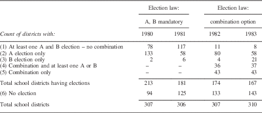
We provide summary statistics for Oregon school district financial elections during this period in Table 1. In the table, we assign each school district to one of six mutually exclusive categories.
-
1. School districts that had at least one A and B election on the same election date, but no Combination election. Some of these districts had multiple such elections in a given school year, when prior attempts failed. Others could have later held an A election only after defeat of both an A and B proposal. They might also have held a B election only if an A proposal had passed and a B proposal had failed.
-
2. Districts that held only A elections. These were districts in which the entire proposed operating budget qualified for the property tax rebate.
-
3. Districts that held only B elections. In these districts, the reversion spending amount exceeded the amount that qualified for a property tax rebate.
-
4. Districts that held a Combination election and some mix of A and B elections. These districts held multiple elections in a given school year, and at least one of the elections was a Combination. (Combination elections were permitted only for the last two years of this period).
-
5. Districts that held only Combination elections.
-
6. Districts that did not hold elections. The board in these districts chose to operate with Q (or less).
Count of Districts by Election Type, Oregon School Referenda 1980–83

Note: Rows 1–6 are mutually exclusive categories. School districts may hold multiple elections within the same year, potentially of different types. Row 1 includes districts that held at least one A and B election, but no combination election. Rows 2, 3 and 5 include districts that held only A, B or Combination elections. Row 4 includes districts that held a Combination election as well as some A and/or B elections. The Combination option was permitted only in 1982 and 1983.
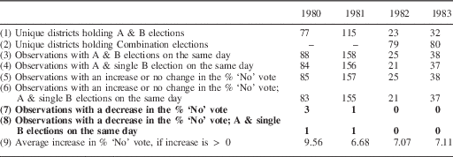
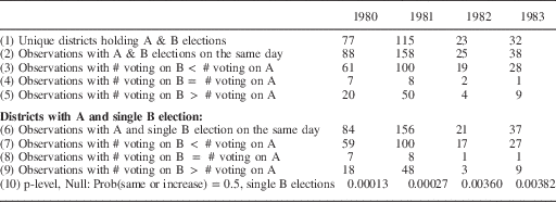
Table 2 provides additional details. The categories in this table are no longer mutually exclusive. The first row shows the total number of school districts that held at least one election with both A and B ballots. The second row shows the number of districts that held at least one Combination election. (Some of these districts also later held simultaneous A and B elections, so the numbers in Row 2 are the sum of Rows 4 and 5 in Table 1). The third row shows the total number of instances in which A and B votes were held on the same day. The numbers in this row exceed those in the first row because some school districts held multiple elections. Some districts held two or three simultaneous A and B elections in the same year.Footnote 9
Oregon School Budget Elections by Type, 1980–83

Note: For Rows 5–9, if multiple B elections were held, the smallest % ‘No’ vote was used in calculating change in the percent voting ‘No’.
School districts were able to hold a single B vote (typical) or two (rare) or more (even rarer) B votes. The multiple votes were presumably to offer a menu of add-ons, such as kindergarten. These votes are not covered by our formal model. Therefore in the fourth row of Table 2 we show the number of observations with an A election and a single B election on the same day (these are a subset of Row 3). As these elections correspond most closely to our model, they constitute our population of interest. As a comparison of the third and fourth rows of Table 2 indicates, multiple B elections were infrequent. Our main results are presented in the remaining rows of the table.
RESULTS
Test of Proposition 1
From Proposition 1, we form the hypothesis that the ‘No’ vote should be greater in the B election than in the A election. We focus on differences in the percentage voting ‘No’ on the B and A votes because there are variations in the number of voters casting A and B ballots.Footnote 10 These variations are relatively small. We report on abstention (in the form of roll-off) in a later section. The fifth row in Table 2 shows the number of observations with an increase in the percentage voting ‘No’ on the B compared to the A ballot (using Row 3 as the baseline population). The sixth row reports observations with an increase in the percentage voting ‘No’ for the subset of observations with a single B election (using Row 4 as the baseline). No change in the votes against is also consistent with the model; this could arise if there were no voters of preference type A ≻ Q ≻ Z or A ≻ Z ≻ Q. There are no more than two such observations in 1980, one in each 1981 and 1982, and none in 1983. These come from districts with very small populations, and are included in the counts in Rows 5 and 6.Footnote 11
The errors to the prediction of Proposition 1 are shown in Rows 7 and 8. If we focus on districts with single B elections, there was only one violation of Proposition 1 in 1980. That district had a decrease in the ‘No’ vote of 1.64 percentage points, which is quite small in comparison to the average increase of 9.56 percentage points in that year. There was a single violation in 1981 and none in 1982 or 1983.Footnote 12
In summary, the evidence in support of Proposition 1 is overwhelming. In a total of 298 observations of elections in which there was an A and a single B ballot on the same day, there were only two violations.Footnote 13 It is delightful to find a result where reporting a statistical test would be absurd. In those districts where there was an increase in the percent voting ‘No,’ the increase was substantial, as reported in the ninth row. The average increase ranged from 6.68 percentage points in the 1981 elections to 9.56 in the 1980 elections.
Test of Proposition 2
Proposition 2 predicts that school boards should prefer to conduct Combination ballot elections rather than separate A and B elections. The empirical hypothesis generated by Proposition 2 is that, when the Combination was an option for the school board, we should observe only Combination ballots, A ballots (but no B), and B ballots (but no A). (As we explained above, A ballots alone would be observed if an A ballot sufficed to produce the maximum budget; B ballots alone would be observed if any levy over the reversion would not qualify for a tax subsidy). Thus when the state permitted Combination ballots, there should be a substantial shift away from A and B elections to Combination ballots. The shift is supported by the data. Row 1 of Table 2 shows that the number of school districts holding A and B votes decreased from 115 in 1981 (and 77 in 1980) to only 23 in 1982, before increasing back to 32 in 1983.Footnote 14 Moreover, of the 23 districts that held A and B votes in 1982, 12 had previously tried a Combination ballot in the same year; in 1983, 22 of 32 districts tried a Combination ballot first. Districts holding at least one Combination ballot, on the other hand, numbered 79 in 1982 and 80 in 1983.
Proposition 2 is not supported as overwhelmingly as Proposition 1. With the Combination option available, a few districts continued to go directly to A and B ballots. A few more reverted to A and B after Combination ballots failed. The model of Romer and Rosenthal (Reference Romer and Rosenthal1979) would argue that, in a situation with a single proposal amount (as is the case with the Combination ballot), budget-maximizing agenda setters would make a relatively high proposal initially and then cut it after a failure. Perhaps switching from Combination to A and B represents a concession expected by voters in the new institutional framework established by the property tax rebate system.Footnote 15 In any event, even though Combination ballots were not adopted uniformly, there was a strong tendency to substitute Combination ballots for A and B ballots. This tendency was especially strong on the first annual election in the district. Proposition 2 is consistent with the drop in A and B elections between the first two years and the second two years.
Proposition 2 also implies that, ceteris paribus, districts holding A and B elections on their first attempt in 1981 would hold a Combination ballot in 1982. An ideal empirical test would be a rerun of school operating budget elections for 1981, with the agenda setter able to make Combination proposals and no longer constrained to make A and B proposals. This repeat experiment would hold underlying voter demand and the reversion constant. Between 1981 and 1982, however, not only demand may have changed but also the reversion, either through the standard augmentation of the 1981 base by 6 percent or through the passage of a new base in 1981. Attempting a full accounting for such factors is outside the scope of this article. Nonetheless, it is instructive to see what districts did in 1982 compared to what they had done in 1981.
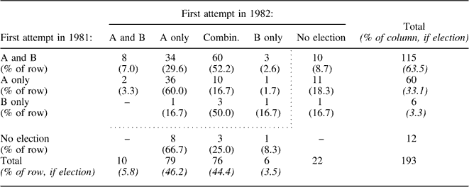
Table 3 provides a summary of the transitions from the 1981 to 1982 elections, by the type of proposal a district made in its first 1981 election. Only districts that held a budget election in either year are included in this table. Far more of the 1981 A and B districts held Combination ballots (52 percent) than repeated A and B (7 percent). In a repeat, districts holding only A elections would be expected to do so again. A majority of such districts did so (60 percent). If such districts continued to hold elections but did not have just an A election, they would be expected to use the Combination. Ten districts held Combination elections (17 percent), while only two held A and B (3 percent) elections. There were relatively few districts in the other two possible types. Considering all districts, we find that 44 percent used Combination ballots on their first attempt in 1982 and only 6 percent used A and B ballots. Even though this 6 percent indicates that Proposition 2 is less uniformly supported than Proposition 1, the strong tendency to replace A and B ballots with Combinations provides support for the model of budget-maximizing agenda setters.
Oregon School Budget Elections by Type in 1981 and 1982

Note: Only districts that held a budget election in 1981 or 1982 are included in this table. Cases inside the dotted lines held a budget election in both 1981 and 1982. “A only (1981)/Combin (1982)” includes one “B and Combin” case for 1982.
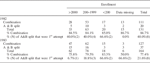
One reason the agenda-setting model may not fully explain changes observed in proposal behavior across these two regimes is that conditions for agenda setting are not uniform across districts. In particular, in large districts, school boards may be more likely to be ‘captured’ by high demanders. Such boards would act as budget maximizers. In small districts, the boards may conform more to the preferences of the median voter (Romer, Rosenthal and Munley Reference Romer, Rosenthal and Munley1992). Oregon has a large number of small rural districts where a shift to Combination budgets from split A and B elections may have been less politically feasible. To examine this possibility, we took a closer look at districts’ propensity to choose a Combination over a split A/B ballot in 1982 and 1983, as it relates to district size (enrollment). The results are shown in Table 4.
Choice of Combination or Split Ballot by District Size, 1982 and 1983

Note: Includes only districts that used either a Combination ballot or one A and one B proposal. Districts that proposed an A ballot only were excluded, as they had no need to make the choice between the two.
We observe that large districts were no more likely than small or medium-sized districts to select a Combination ballot rather than the two-proposal A/B ballot, in either year. In both years a probit model for the choice of a Combination ballot over and A/B finds a small positive, but statistically insignificant, relationship between district size and the use of a Combination proposal (results are not shown, but are available from the authors). The relationship is more evident when focusing on first election attempts in 1983, in which most of the A/B split ballots in large districts were on a later attempt, not the first one. Among smaller districts, A/B split ballots were more common on the first attempt.
ABSTENTION (ROLL-OFF) WHEN A AND B PROPOSALS ARE BOTH ON THE BALLOT
As we have noted, voters did not always vote on both the A and B proposals when both appeared on the ballot. Although the differences in votes cast in the two elections are small, the differences are systematic.
The differences do not appear to be explained by the purely random turnout model of Romer and Rosenthal (Reference Romer and Rosenthal1979). The voters have taken the trouble to vote; they should be no more likely to ‘forget’ to vote on one of the two proposals than the other or to make a ‘mistake’ and abstain. Consequently, differences in turnout should not be systematic. Under random abstention, the number voting on the A amount should exceed those voting on the B amount about half the time, and vice versa. The differences would also seem to be unrelated to the strategic turnout models based on the cost of voting (Palfrey and Rosenthal Reference Palfrey and Rosenthal1985). The voters, by getting a ballot, have paid the cost of voting.
What might be relevant to the turnout differences is informational uncertainty about preferences (Feddersen and Pesendorfer Reference Feddersen and Pesendorfer1997, Reference Feddersen and Pesendorfer1999). A voter might not be sufficiently informed, say, to know whether he has preference Z ≻ A ≻ Q or A ≻ Z ≻ Q. This voter knows he should vote for A, but is unsure about whether to vote for B. Such a voter might abstain strategically and leave the decision to informed voters. Alternatively, the voter might be close to indifferent between A and Z. In such a case, he or she might abstain due to indifference (Hinich and Ordeshook Reference Hinich and Ordeshook1969). What we have in mind here is not “I’m close to indifferent, so I do not want to pay the cost of voting,” as in Riker and Ordeshook’s seminal 1968 article. It is more “I’m close to indifferent, and I can’t make up my mind, so I’ll just pass on this one.”
A strong empirical relationship with regard to votes cast is shown in Table 5. In all four years, the number of districts in which there were fewer votes on the B proposal than on the A far exceeds the number of districts in which the opposite is true. The last row of the table presents a simple binomial test of the null hypothesis that votes in the B election are fewer than those in A elections with probability 0.5. That is, for this test if fewer votes are cast in the B election it is considered a ‘success’ and more votes or no change is a ‘failure.’ The test is run only for districts that did not split their B ballots into two or more pieces. For each year, the null is rejected with p-values lower than 0.005.
Differences in Voter Turnout between A and B Ballots

CONCLUSION
We have presented evidence that voters, at least in the aggregate, vote rationally when presented with a budget proposal and an ‘add-on’ second proposal. Under the assumption that voters have single-peaked preferences regarding spending, we should systematically find more votes against the second proposal than against the first. This proposition is overwhelmingly verified. Another observation pointed to systematic behavior by budget-maximizing agenda setters. When given the option of not having two proposals and proposing just a single budget, the setters should opt for the single proposal. Indeed, they did so, with relatively few exceptions. Voters do vary, however, in their participation when voting on two proposals. Second proposals typically have fewer voters than first proposals, at high levels of statistical significance.
The results in this article are in the spirit of Romer and Rosenthal (Reference Romer and Rosenthal1979), who presented a theoretical model of budget-maximizing agenda setting along with qualitative evidence that was consistent with the model. Their model also made quantitative predictions about the amounts of the proposals and the percentage of voters that should support a proposal. These predictions were then tested in a series of later articles (Romer and Rosenthal Reference Romer and Rosenthal1982a, Reference Romer and Rosenthal1982b; Filimon, Romer and Rosenthal Reference Filimon, Romer and Rosenthal1982). The two-proposal scenario will similarly generate a set of quantitative predictions about budget proposals and voting. These predictions will have to account for the endogeneity of tax price (see Romer, Rosenthal and Munley Reference Romer, Rosenthal and Munley1992) induced by the A and B setup. The various predictions generated by the A and B setup can be pursued in further research.