2.1 Physical model

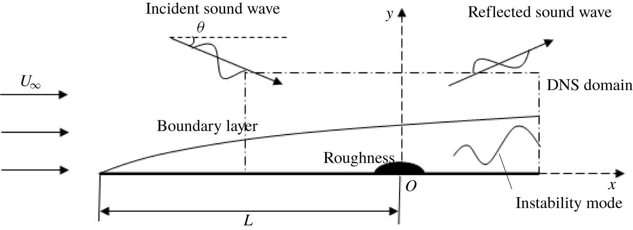
As is sketched in figure 1, the physical model to be studied is a two-dimensional (2-D) supersonic boundary layer forming over a flat plate. For convenience, we assume that the plate is isothermal, but the theories also apply to adiabatic walls if the wall temperature condition is changed accordingly. The oncoming fluid is assumed to be a perfect gas, and its viscosity satisfies Sutherland’s law. A 3-D sound wave originating from a distant source propagates at an incident angle $\unicode[STIX]{x1D703}$ towards the boundary layer, and is reflected due to the presence of the boundary layer. Here, the incident angle is defined as

(2.1)$$\begin{eqnarray}\unicode[STIX]{x1D703}=\cos ^{-1}\left[\unicode[STIX]{x1D6FC}_{a,r}^{\ast }/\sqrt{(\unicode[STIX]{x1D6FC}_{a,r}^{\ast })^{2}+(\unicode[STIX]{x1D6FE}_{a}^{\ast })^{2}+(\unicode[STIX]{x1D6FD}_{a}^{\ast })^{2}}\right],\end{eqnarray}$$

where $\unicode[STIX]{x1D6FC}_{a}^{\ast }$, $\unicode[STIX]{x1D6FE}_{a}^{\ast }$ and $\unicode[STIX]{x1D6FD}_{a}^{\ast }$ are the dimensional streamwise, wall-normal and spanwise wavenumbers of the acoustic wave, respectively, and the subscripts $r$ and $i$ throughout the paper denote the real and imaginary parts, respectively. We focus on the spatially evolving case, for which $\unicode[STIX]{x1D6FE}_{a}^{\ast }$ and $\unicode[STIX]{x1D6FD}_{a}^{\ast }$ are real, and $\unicode[STIX]{x1D6FC}_{a}^{\ast }$ is complex with a small damping rate due to viscosity. An array of 3-D spanwise periodic and streamwise isolated roughness elements is located at a distance $L$ downstream of the leading edge. The interactions of the acoustic-driven unsteady fluctuation with the roughness and with the local mean flow lead to generation of an instability mode downstream.

Figure 1.

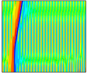
Sketch of the physical model. Both the incident wave and the roughness can be three-dimensional, and a cross-section in the $x{-}y$ plane is illustrated.

We define the characteristic length as the local boundary-layer characteristic thickness $\unicode[STIX]{x1D6FF}=\sqrt{\unicode[STIX]{x1D708}_{\infty }L/U_{\infty }}$, where the subscript $\infty$ indicates a quantity of the oncoming flow, and $U$ and $\unicode[STIX]{x1D708}$ represent the velocity and the kinematic viscosity, respectively. The flow is to be described in the Cartesian coordinate system $(x,y,z)$, with its origin located at the roughness centre; the spatial and time variables are introduced as $(x,y,z)=(x^{\ast },y^{\ast },z^{\ast })/\unicode[STIX]{x1D6FF}$ and $t=t^{\ast }U_{\infty }/\unicode[STIX]{x1D6FF}$, respectively, where the asterisk denotes a dimensional quantity throughout this paper. For simplicity, we assume the spanwise distribution of the roughness to be a cosine function. The surface of the roughness is specified as

(2.2)$$\begin{eqnarray}y=hf(x)(\text{e}^{\text{i}k_{z}z}+\text{e}^{-\text{i}k_{z}z})/2=hf(x)\cos (k_{z}z),\end{eqnarray}$$

where $h$ characterises the roughness height, $k_{z}$ is the spanwise wavenumber and $f(x)$ is the shape function normalised by its peak value (i.e. $\max |f(x)|=1$). The velocity field, density, temperature and pressure are normalised by their free-stream quantities,

$$\begin{eqnarray}(u,v,w,\unicode[STIX]{x1D70C},T,p)=(u^{\ast }/U_{\infty },v^{\ast }/U_{\infty },w^{\ast }/U_{\infty },\unicode[STIX]{x1D70C}^{\ast }/\unicode[STIX]{x1D70C}_{\infty },T^{\ast }/T_{\infty },p^{\ast }/(\unicode[STIX]{x1D70C}_{\infty }U_{\infty }^{2})).\end{eqnarray}$$

We define the Reynolds number $R$ and the oncoming Mach number $M$ as

(2.3a,b)$$\begin{eqnarray}R=U_{\infty }\unicode[STIX]{x1D6FF}/\unicode[STIX]{x1D708}_{\infty }=\sqrt{U_{\infty }L/\unicode[STIX]{x1D708}_{\infty }},\quad M=U_{\infty }/a_{\infty },\end{eqnarray}$$

where $a$ is the sound speed. We assume that $R\gg 1$ in the asymptotic analysis, and our interest is in the supersonic regime with $M>1$, but the hypersonic regime for $M>5$ is also covered in our theory. The case studies will cover both regimes.

In this paper, we restrict our attention to the inviscid modes, which include, according to Smith (Reference Smith1989), almost all instability modes except the first modes with small frequencies $\unicode[STIX]{x1D714}^{\ast }\leqslant O(R^{-1/2}U_{\infty }/\unicode[STIX]{x1D6FF})$ and large obliqueness angles

(2.4)$$\begin{eqnarray}\unicode[STIX]{x1D6E9}\equiv \tan ^{-1}(\unicode[STIX]{x1D6FD}^{\ast }/\unicode[STIX]{x1D6FC}^{\ast })>\unicode[STIX]{x1D6E9}_{0}=\tan ^{-1}(\sqrt{M^{2}-1}),\end{eqnarray}$$

where $\unicode[STIX]{x1D6FC}^{\ast }$ and $\unicode[STIX]{x1D6FD}^{\ast }$ are the dimensional streamwise and spanwise wavenumbers, respectively. Inviscid modes have dimensional phase speeds and frequencies of $O(U_{\infty })$ and $O(U_{\infty }/\unicode[STIX]{x1D6FF})$, respectively, and their wavelengths are thus comparable with the local boundary-layer thickness $\unicode[STIX]{x1D6FF}$. The characteristic width of the roughness is taken to be of $O(\unicode[STIX]{x1D6FF})$, in order to satisfy the ‘resonance condition’, or ‘scale matching’, as is required by receptivity.

Figure 2.

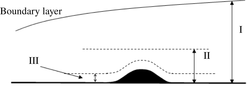
Asymptotic structure of the receptivity problem. Region I: inviscid main layer (of $O(\unicode[STIX]{x1D6FF})$), region II: wall layer (of $O(R^{-1/3}\unicode[STIX]{x1D6FF})$), region III: viscous Stokes layer (of $O(R^{-1/2}\unicode[STIX]{x1D6FF})$).

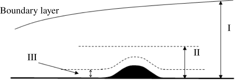
If the roughness has a height of $O(R^{-1/3}\unicode[STIX]{x1D6FF})$ or smaller, then the mean-flow distortion is governed by a double-deck structure, consisting of the main layer with $O(\unicode[STIX]{x1D6FF})$ width and a much thinner wall layer in an $O(R^{-1/3}\unicode[STIX]{x1D6FF})$ vicinity of the wall surface; see regions I and II of figure 2, respectively. The mathematical description for the incompressible regime was provided by Choudhari & Duck (Reference Choudhari and Duck1996). A direct consequence is that the mean-flow distortion in the main layer is of $O(hR^{-1/3})$. As the simplest set-up, we assume that the roughness height is at most comparable with the thickness of the wall layer, i.e.

(2.5)$$\begin{eqnarray}h\leqslant O(R^{-1/3}).\end{eqnarray}$$

2.2 The local receptivity mechanism: general description and asymptotic estimate

Figure 3.

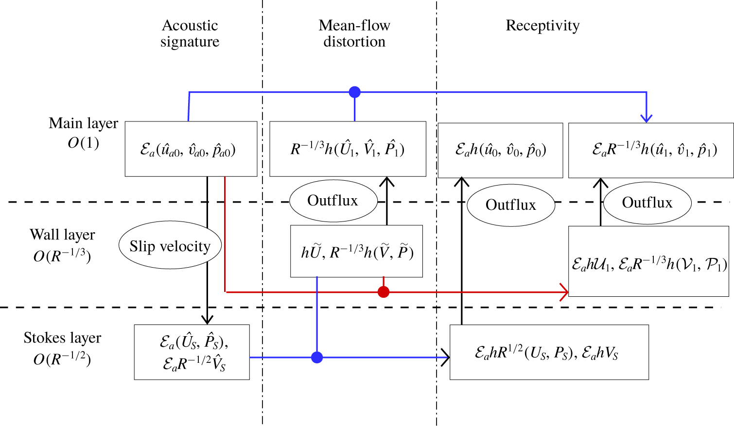
An illustration of the key excitation processes in the local receptivity mechanism.

The local receptivity mechanism is, roughly speaking, rather simple: the acoustic signature driven by the free-stream sound wave and the local mean-flow distortion caused by the roughness interact with each other to produce a forcing, which has a frequency and length scale comparable with those of the inviscid instability, and therefore excites an eigenmode. However, it turns out that the acoustic disturbance also interacts directly with the roughness to generate the dominant forcing. This aspect and further insights can be gained by examining the key processes involved from the perspective of asymptotic approximation. This allows us to identify the leading- and second-order interactions, and to estimate their contributions to the receptivity, as is illustrated in figure 3, where the arrows indicate the interplay between different layers. If the incident acoustic wave has a sufficiently small amplitude ${\mathcal{E}}_{a}\ll 1$ and an $O(U_{\infty }/\unicode[STIX]{x1D6FF})$ frequency, then the boundary-layer response in the main layer is linear and inviscid, and corresponds to an acoustic-branch continuous mode of the compressible Rayleigh equation. The balance in the Rayleigh equation determines that the velocity and pressure fluctuations are of $O({\mathcal{E}}_{a})$. However, the absence of the viscous effect implies a non-zero slip velocity at the bottom of this layer. In order to satisfy the no-slip velocity at the wall, a Stokes layer with a thickness of $O(R^{-1/2}\unicode[STIX]{x1D6FF})$ needs to be introduced, which is shown as region III in figure 2. The balance in the Stokes layer shows that the streamwise velocity and pressure remain of $O({\mathcal{E}}_{a})$, but the transverse velocity drops to $O({\mathcal{E}}_{a}R^{-1/2})$. The viscous displacement induces a streamwise-uniform $O({\mathcal{E}}_{a}R^{-1/2})$ transpiration velocity at the outer edge of the Stokes layer, thereby producing an $O({\mathcal{E}}_{a}R^{-1/2})$ correction to the main-layer perturbation. This $O({\mathcal{E}}_{a}R^{-1/2})$ correction only represents the acoustic signature in the ‘flat’ boundary layer, and does not contribute to the local receptivity. Crucially, as the Stokes layer develops on the curved surface of the roughness, a much larger streamwise velocity $\tilde{u} =O({\mathcal{E}}_{a}hR^{1/2})$ is induced to satisfy the no-slip condition, ${\mathcal{E}}_{a}U_{S}+\tilde{u} \approx 0$ at $y=hf(x)\cos (k_{z}z)$. Here, the order of magnitude follows from the Taylor expansion of the left-hand side about $y=0$, $[{\mathcal{E}}_{a}(\unicode[STIX]{x2202}U_{S}/\unicode[STIX]{x2202}y)h\cos (k_{z}z)+\tilde{u} ]_{y=0}\approx 0$. It transpires that $\tilde{u}$ must be of $O({\mathcal{E}}_{a}hR^{1/2})$ due to the steep $O(R^{1/2})$ gradient of $U_{S}$, $\unicode[STIX]{x2202}U_{S}/\unicode[STIX]{x2202}y$. The continuity equation indicates that the associated transverse velocity is $O({\mathcal{E}}_{a}h)$, and remains of this size at the outer edge of the Stokes layer. This $O({\mathcal{E}}_{a}h)$ unsteady and streamwise-dependent outflux acts on the main layer as the equivalent local suction/blowing to generate an $O({\mathcal{E}}_{a}h)$ perturbation, from which a discrete mode of the same order of magnitude will emerge downstream. On the other hand, the roughness induces $O(h)$ and $O(R^{-1/3}h)$ streamwise and transverse velocities in the viscous wall layer. The $O(R^{-1/3}h)$ outflux drives an $O(R^{-1/3}h)$ steady perturbation in the main layer, where this perturbation interacts with the $O({\mathcal{E}}_{a})$ acoustic signature, producing a volumetric unsteady forcing of $O({\mathcal{E}}_{a}R^{-1/3}h)$. In addition, the mean flow in the viscous wall layer interacts with the $O({\mathcal{E}}_{a})$ acoustic fluctuation to produce an $O({\mathcal{E}}_{a}R^{-1/3}h)$ outflux. These estimates hold even when $h=O(R^{-1/3})$. The rough estimate made in the introduction only took the second-order effect into account and thus underestimated the coupling coefficient.

Fortunately, the two excitation processes operate completely independently, and can therefore be accounted for separately. This implies that these two orders of approximations may be reversed in some extreme cases, as will be illustrated later. Of course, the two processes may interact with each other at higher orders, generating even smaller corrections, the inclusion of which is beyond the scope of the present paper.

The leading-order contribution to the receptivity depends therefore only on the deformation of the sound-generated Stokes layer by the curved wall. Moreover, it will be shown to be equivalent to the simplest receptivity, i.e. excitation of instability modes by time-periodic blowing and suction through a slot on the wall. The latter problem serves as an elementary building block for the more complicated ones. It can be formulated in either the finite-$R$ or high-$R$ asymptotic framework. Appendix C presents the analysis and results of this suction-induced receptivity, and demonstrates its link with the present receptivity due to the roughness–sound interaction.

3.1 Mean-flow distortion

The solutions for the steady and unsteady perturbations can be obtained by Fourier transform with respect to $x$, defined as

(3.4)$$\begin{eqnarray}\mathscr{F}[\cdot ](k_{x})\equiv \frac{1}{\sqrt{2\unicode[STIX]{x03C0}}}\int _{-\infty }^{\infty }\cdot \exp (-\text{i}k_{x}x)\,\text{d}x,\end{eqnarray}$$

where the dot represents a function in physical space and $k_{x}$ the streamwise wavenumber. Substituting (3.3) into the compressible Navier–Stokes equations, neglecting the $O(h^{2})$ terms and performing the Fourier transform, we arrive at the steady, compressible Orr–Sommerfeld equations

(3.5)$$\begin{eqnarray}\unicode[STIX]{x1D647}_{OS}(d_{y};\unicode[STIX]{x1D714}=0,k_{x},k_{z},R)\hat{\unicode[STIX]{x1D731}}_{w}=0,\end{eqnarray}$$

where $\hat{\unicode[STIX]{x1D731}}_{w}(k_{x},y)=\mathscr{F}[\bar{\unicode[STIX]{x1D731}}_{w}(x,y)]$ and $\unicode[STIX]{x1D647}_{OS}(d_{y};\unicode[STIX]{x1D714},k_{x},k_{z},R)$ is an $8\times 8$-order matrix differential operator (also referred to as the O–S operator) with $\unicode[STIX]{x1D714}$, $k_{x}$ and $k_{z}$ being the frequency, streamwise wavenumber and spanwise wavenumber, respectively. The operator $\unicode[STIX]{x1D647}_{OS}$ in the present paper is equivalent to $\unicode[STIX]{x1D644}d_{y}-\boldsymbol{A}$ in Malik (Reference Malik1990) with $\unicode[STIX]{x1D644}$ being the unity matrix.

The wall boundary conditions read,

(3.6a-c)$$\begin{eqnarray}U_{B}+h\bar{U}_{w}=0,\quad T+h\bar{T}_{w}=T_{w},\quad \bar{V}_{w}=\bar{W}_{w}=0\quad \text{at}~y=hf(x).\end{eqnarray}$$

Performing first-order Taylor expansion about $y=0$ for $h\ll 1$, and then taking Fourier transform, we obtain the inhomogeneous boundary conditions on the flat wall,

(3.7a,b)$$\begin{eqnarray}(\hat{U} _{w},\hat{T}_{w})=-(U_{B}^{\prime }(0),T_{B}^{\prime }(0))\hat{f}(k_{x}),\quad \hat{V}_{w}={\hat{W}}_{w}=0\quad \text{at}~y=0,\end{eqnarray}$$

where $\hat{U} _{w}$, $\hat{V}_{w}$, ${\hat{W}}_{w}$ and $\hat{T}_{w}$ are components of $\hat{\unicode[STIX]{x1D731}}_{w}$, and $\hat{f}(k_{x})=\mathscr{F}[f(x)]$. In the uniform inviscid flow outside of the boundary layer (i.e. $y\rightarrow \infty$), the solution for $\hat{\unicode[STIX]{x1D731}}_{w}$ can be expressed as a linear superposition of complementary solutions,

(3.8)$$\begin{eqnarray}\hat{\unicode[STIX]{x1D731}}_{w}=\mathop{\sum }_{l=1}^{8}a^{(l)}\unicode[STIX]{x1D709}^{(l)}\text{e}^{\unicode[STIX]{x1D706}_{l}y},\end{eqnarray}$$

where $a^{(l)}$ are constants, and $\unicode[STIX]{x1D706}_{l}$ and $\unicode[STIX]{x1D709}^{(l)}$ denote the eigenvalue and eigenfunction of the operator $\unicode[STIX]{x1D647}_{OS}(\unicode[STIX]{x1D706};\unicode[STIX]{x1D714}=0,k_{x},k_{z},R)$ in which $\unicode[STIX]{x1D706}$ takes the place of $d_{y}$. The eigenvalues $\unicode[STIX]{x1D706}_{l}$ appear in pairs, i.e.

(3.9)$$\begin{eqnarray}\unicode[STIX]{x1D706}_{1}=-\unicode[STIX]{x1D706}_{2}=\text{i}[k_{x}^{2}(M^{2}-1)-k_{z}^{2}]^{1/2}+O(R^{-1}),\quad \unicode[STIX]{x1D706}_{3,5,7}=-\unicode[STIX]{x1D706}_{4,6,8}.\end{eqnarray}$$

For $|k_{z}/k_{x}|<\sqrt{M^{2}-1}$, only $\unicode[STIX]{x1D706}_{1,2}$ are purely imaginary to leading-order accuracy, and the real parts of $\unicode[STIX]{x1D706}_{3,5,7}$ are taken to be positive. The expressions of $\unicode[STIX]{x1D706}_{l}$ are the same as (2.20)–(2.26) in Balakumar & Malik (Reference Balakumar and Malik1992) provided that we set $\unicode[STIX]{x1D714}=0$. Note that the complementary solutions corresponding to $\unicode[STIX]{x1D709}^{(1)}$ and $\unicode[STIX]{x1D709}^{(2)}$ represent the incoming and outgoing perturbations propagating along the two characteristics in the supersonic uniform stream. Since the perturbation originates from the wall, the exponentially growing and the incoming components should all be removed by setting

(3.10)$$\begin{eqnarray}\displaystyle & a^{(1)}=a^{(3)}=a^{(5)}=a^{(7)}=0\quad \text{for}~k_{x}>0, & \displaystyle\end{eqnarray}$$

(3.11)$$\begin{eqnarray}\displaystyle & a^{(2)}=a^{(3)}=a^{(5)}=a^{(7)}=0\quad \text{for}~k_{x}<0. & \displaystyle\end{eqnarray}$$

The outgoing component represents a Mach wave radiated to the far field. Since $\hat{\unicode[STIX]{x1D731}}_{w}$ is proportional to $\hat{f}(k_{x})$, $\hat{\unicode[STIX]{x1D731}}_{w}/\hat{f}(k_{x})$ depends on $y$ only. The boundary-value problem consisting of (3.5), (3.7) and (3.8) with (3.10) or (3.11) is solved using the O–S solver that was used in a few previous papers, e.g. Dong & Wu (Reference Dong and Wu2013), Wu & Dong (Reference Wu and Dong2016a).

3.2 Acoustic signature and instability modes

The compressible O–S equations admit a family of continuous modes satisfying the acoustic dispersion relation in the free stream. Each of these modes represents an incident sound wave and its signature in the boundary layer. The O–S equations also have vortical and entropy branches of continuous modes. However, as was pointed out by Dong & Wu (Reference Dong and Wu2013) and Wu & Dong (Reference Wu and Dong2016a), neither of them represents the physical free-stream vortical/entropy disturbances or their entrainment into the boundary layer because the latter are influenced at leading order by non-parallelism, which is neglected in the O–S equations. The discrete mode of the O–S equations corresponds to the boundary-layer instability mode. The acoustic perturbation and the discrete mode can be expressed as

(3.12)$$\begin{eqnarray}\tilde{\unicode[STIX]{x1D731}}_{a,I}={\mathcal{E}}_{a,I}\hat{\unicode[STIX]{x1D731}}_{a,I}(y)\exp [\text{i}(\unicode[STIX]{x1D6FC}_{a,I}x+\unicode[STIX]{x1D6FD}_{a,I}z-\unicode[STIX]{x1D714}_{a,I}t)]+\text{c.c.},\end{eqnarray}$$

where the subscripts $a$ and $I$ refer to the acoustic perturbation and the instability mode, respectively, and ${\mathcal{E}}\ll 1$ is the amplitude. For a spatially evolving perturbation, $\unicode[STIX]{x1D6FC}_{a}$ has an $O(R^{-1})$ damping rate, but $\unicode[STIX]{x1D6FC}_{I}$ may have an $O(1)$ positive or negative imaginary part.

Under the parallel-flow assumption, both of them satisfy the O–S equations

(3.13)$$\begin{eqnarray}\unicode[STIX]{x1D647}_{OS}\hat{\unicode[STIX]{x1D731}}_{l}=0\quad (l=a,I),\end{eqnarray}$$

subject to no-slip $\hat{u} _{l}(0)={\hat{w}}_{l}(0)=0$, non-penetration $\hat{v}_{l}(0)=0$ and isothermal $\hat{\unicode[STIX]{x1D703}}_{l}(0)=0$ (with $\unicode[STIX]{x1D703}$ representing the temperature perturbation) boundary conditions at the wall. However, the far-field boundary conditions are different.

For a continuous mode $\tilde{\unicode[STIX]{x1D731}}_{a}$, an inhomogeneous forcing is imposed in the free stream. The solution of the O–S equations in a uniform stream is a superposition of eight (or four pairs of) complementary solutions; see (2.19) in Balakumar & Malik (Reference Balakumar and Malik1992). For an acoustic-branch mode, only one pair of the complementary solutions are oscillatory; of the remaining six, three decay exponentially while the other three amplify exponentially as $y\rightarrow \infty$. The far-field boundary conditions must be such that the coefficients of the three exponentially growing complementary solutions be set to zero, and a certain normalisation condition be imposed. Therefore, the pressure perturbation in the free stream, for instance, is expressed as

(3.14)$$\begin{eqnarray}\hat{p}_{a}(y)\rightarrow I_{a}\text{e}^{\text{i}\unicode[STIX]{x1D6FE}_{a}y}+R_{a}\text{e}^{-\text{i}\unicode[STIX]{x1D6FE}_{a}y}+\mathop{\sum }_{l=1}^{3}{\mathcal{D}}_{l}\text{e}^{-\unicode[STIX]{x1D70E}_{l}y}\quad \text{as}~y\rightarrow \infty ,\end{eqnarray}$$

where $I_{a}$ and $R_{a}$ represent the amplitudes of the incident and reflected sound waves, respectively, and $\unicode[STIX]{x1D70E}_{l}$ (whose real part is positive) and ${\mathcal{D}}_{l}$ are the decaying rate and amplitude of the complementary solutions trapped within the boundary layer. As a normalisation, we simply take the pressure amplitude of the incident sound wave to be unity, i.e. $I_{a}=1$. Other quantities can be derived from the linearised Euler equations.

Substituting (3.14) into the linearised N–S equations and dropping the exponentially small terms lead to the acoustic dispersion relation,

(3.15)$$\begin{eqnarray}\unicode[STIX]{x1D714}_{a}=\left(1\pm \frac{1}{M\cos \unicode[STIX]{x1D703}}\right)\unicode[STIX]{x1D6FC}_{a}+O(R^{-1}),\end{eqnarray}$$

where the ‘+’ and ‘-’ signs represent the fast and slow acoustic waves, respectively, and the incident angle $\unicode[STIX]{x1D703}$ has been defined in (2.1). We take $\unicode[STIX]{x1D703}\in [0,\unicode[STIX]{x03C0}/2)$ for a fast acoustic wave and $\unicode[STIX]{x1D703}\in [0,\cos ^{-1}(1/M))$ for a slow acoustic wave. The incident wave should have a negative group velocity in the wall-normal direction, i.e. $\text{d}\unicode[STIX]{x1D714}/\text{d}\unicode[STIX]{x1D6FE}_{a}<0$, therefore, $\unicode[STIX]{x1D6FE}_{a}$ is positive for a slow acoustic wave but negative for a fast acoustic wave.

The eigenfunction of the discrete mode $\tilde{\unicode[STIX]{x1D731}}_{I}$ decays exponentially in the external stream, i.e. $\hat{\unicode[STIX]{x1D731}}_{I}\rightarrow 0$ as $y\rightarrow \infty$. It is normalised by setting the wall pressure to unity, i.e. $\hat{p}_{I}(0)=1$. For brevity, from here onwards, we denote $\unicode[STIX]{x1D6FC}_{I}$, $\unicode[STIX]{x1D6FD}_{I}$ and $\unicode[STIX]{x1D714}_{I}$ as $\unicode[STIX]{x1D6FC}$, $\unicode[STIX]{x1D6FD}$ and $\unicode[STIX]{x1D714}$, respectively.

3.3 Scattering of the acoustic signature by the roughness-induced mean-flow distortion

When both the free-stream acoustic wave and wall roughness are present, the unsteady perturbation is expressed as

(3.16)$$\begin{eqnarray}\tilde{\unicode[STIX]{x1D731}}={\mathcal{E}}_{a}[\hat{\unicode[STIX]{x1D731}}_{a}(y)\text{e}^{\text{i}(\unicode[STIX]{x1D6FC}_{a}x+\unicode[STIX]{x1D6FD}_{a}z)}+h\tilde{\unicode[STIX]{x1D731}}_{1}(x,y)\text{e}^{\text{i}\unicode[STIX]{x1D6FD}z}/2]\text{e}^{-\text{i}\unicode[STIX]{x1D714}t}+\text{c.c.},\end{eqnarray}$$

where $\unicode[STIX]{x1D714}=\unicode[STIX]{x1D714}_{a}$ and $\unicode[STIX]{x1D6FD}=\unicode[STIX]{x1D6FD}_{a}+k_{z}$. Substituting (3.16) into the compressible N–S equations, and neglecting the non-parallelism of the base flow, we obtain at $O({\mathcal{E}}_{a}h)$, the equations governing $\tilde{\unicode[STIX]{x1D731}}_{1}$, which are Fourier transformed with respect to $x$, leading to the inhomogeneous linearised system,

(3.17)$$\begin{eqnarray}\unicode[STIX]{x1D647}_{OS}(d_{y};\unicode[STIX]{x1D714},k,\unicode[STIX]{x1D6FD},R)\hat{\unicode[STIX]{x1D731}}_{1}(k,y)=\boldsymbol{F}[\hat{\unicode[STIX]{x1D731}}_{w}(k_{x},y),\hat{\unicode[STIX]{x1D731}}_{a}(y)],\end{eqnarray}$$

where $\hat{\unicode[STIX]{x1D731}}_{1}=\mathscr{F}[\tilde{\unicode[STIX]{x1D731}}_{1}]$, $k=\unicode[STIX]{x1D6FC}_{a}+k_{x}$ and $\boldsymbol{F}$ denotes the interaction between the mean-flow distortion and the acoustic signature. The detailed expression of $\boldsymbol{F}$ is given in appendix A. The attenuation condition $\hat{\unicode[STIX]{x1D731}}_{1}|_{y\rightarrow \infty }\rightarrow 0$ also holds. An inhomogeneous boundary condition arises due to the deformation of the acoustic signature at the curved wall,

(3.18)$$\begin{eqnarray}(\hat{u} _{1},\hat{v}_{1},{\hat{w}}_{1},\hat{\unicode[STIX]{x1D703}}_{1})=-(\hat{u} _{a,y}(0),\hat{v}_{a,y}(0),{\hat{w}}_{a,y}(0),\hat{\unicode[STIX]{x1D703}}_{a,y}(0))\hat{f}(k_{x})\quad \text{at}~y=0,\end{eqnarray}$$

which is given by Taylor expansion of the no-slip and isothermal conditions on the wall.

The solution for $\tilde{\unicode[STIX]{x1D731}}_{1}$ in physical space is obtained by inverting the Fourier transform,

(3.19)$$\begin{eqnarray}\tilde{\unicode[STIX]{x1D731}}_{1}(x,y)=\mathscr{F}^{-1}[\hat{\unicode[STIX]{x1D731}}_{1}(k,y)]\equiv \frac{1}{\sqrt{2\unicode[STIX]{x03C0}}}\int _{-\infty }^{\infty }\hat{\unicode[STIX]{x1D731}}_{1}(k,y)\text{e}^{\text{i}kx}\,\text{d}k.\end{eqnarray}$$

The integrand has a pole at $k=\unicode[STIX]{x1D6FC}$, where $\unicode[STIX]{x1D6FC}$ is the wavenumber of a discrete mode. The integral in (3.19) may be evaluated by closing the integration contour in the upper half of the complex $k$-plane (Goldstein Reference Goldstein1985; Choudhari & Streett Reference Choudhari and Streett1992; Crouch Reference Crouch1992). The inverse Fourier integral corresponds to a sum of contributions from the poles and the branch cuts of the integrand $\hat{\unicode[STIX]{x1D731}}_{1}$. The contribution from the latter represents the near field in the vicinity of the roughness, and decays algebraically as $x\rightarrow \pm \infty$. The disturbance sufficiently downstream is dominated by the contribution from the pole, which is evaluated by using the residual theorem. It follows that

(3.20)$$\begin{eqnarray}\tilde{\unicode[STIX]{x1D731}}_{1}(x,y)\rightarrow \frac{\sqrt{2\unicode[STIX]{x03C0}}\text{i}}{[\unicode[STIX]{x2202}(\hat{\unicode[STIX]{x1D731}}_{1})^{-1}/\unicode[STIX]{x2202}k]_{k=\unicode[STIX]{x1D6FC}}}\text{e}^{\text{i}\unicode[STIX]{x1D6FC}x}\quad \text{as}~x\rightarrow \infty ,\end{eqnarray}$$

where the notation $(\hat{\unicode[STIX]{x1D731}}_{1})^{-1}$ for a vector $\hat{\unicode[STIX]{x1D731}}_{1}$ is a vector with each component being the reciprocal of the corresponding component in $\hat{\unicode[STIX]{x1D731}}_{1}$. The right-hand side of (3.20) stands for the eigenmode excited, with the prefactor of $\text{e}^{\text{i}\unicode[STIX]{x1D6FC}x}$ representing the equivalent amplitude at the roughness centre.

An explanation of how to evaluate the denominator is in order. This involves solving the inhomogeneous O–S equations (3.17) at two perturbed wavenumbers $k=\unicode[STIX]{x1D6FC}\pm \unicode[STIX]{x1D6E5}_{\unicode[STIX]{x1D6FC}}$ with $\unicode[STIX]{x1D6E5}_{\unicode[STIX]{x1D6FC}}\ll 1$, to obtain $\hat{\unicode[STIX]{x1D731}}_{1}(\unicode[STIX]{x1D6FC}\pm \unicode[STIX]{x1D6E5}_{\unicode[STIX]{x1D6FC}})$ and $(\hat{\unicode[STIX]{x1D731}}_{1})^{-1}$. Then $[\unicode[STIX]{x2202}(\hat{\unicode[STIX]{x1D731}}_{1})^{-1}/\unicode[STIX]{x2202}k]_{k=\unicode[STIX]{x1D6FC}}$ is calculated by a central difference scheme. Such a procedure is an extension of Choudhari & Streett (Reference Choudhari and Streett1992) and Crouch (Reference Crouch1992) to the supersonic regime. Since both the right-hand side of (3.17) and the boundary condition (3.18) are proportional to $\hat{f}(k_{x})$, $\tilde{\unicode[STIX]{x1D731}}_{1}$ depends on $\hat{f}(k_{x})=\hat{f}(\unicode[STIX]{x1D6FC}-\unicode[STIX]{x1D6FC}_{a})$ linearly. Taking the wall pressure as a measure of the amplitude of the mode excited, we further introduce the receptivity efficiency function,

(3.21)$$\begin{eqnarray}\unicode[STIX]{x1D6EC}_{OS}=\frac{1}{\hat{f}(\unicode[STIX]{x1D6FC}-\unicode[STIX]{x1D6FC}_{a})}\lim _{x\rightarrow \infty }\tilde{p}_{1}(x,0)\text{e}^{-\text{i}\unicode[STIX]{x1D6FC}x}=\frac{\sqrt{2\unicode[STIX]{x03C0}}\text{i}}{\hat{f}(\unicode[STIX]{x1D6FC}-\unicode[STIX]{x1D6FC}_{a})[\unicode[STIX]{x2202}\hat{p}_{1}^{-1}(k,0)/\unicode[STIX]{x2202}k]_{k=\unicode[STIX]{x1D6FC}}},\end{eqnarray}$$

which is independent of the roughness. The downstream perturbation thus reads

(3.22)$$\begin{eqnarray}\tilde{\unicode[STIX]{x1D731}}\rightarrow {\mathcal{E}}_{a}\left[\hat{\unicode[STIX]{x1D711}}_{a}\text{e}^{\text{i}\unicode[STIX]{x1D6FC}_{a}x}+\frac{h}{2}\hat{f}(\unicode[STIX]{x1D6FC}-\unicode[STIX]{x1D6FC}_{a})\unicode[STIX]{x1D6EC}_{OS}\hat{\unicode[STIX]{x1D731}}_{1}\text{e}^{\text{i}\unicode[STIX]{x1D6FC}x}+\cdots \right]\text{e}^{\text{i}(\unicode[STIX]{x1D6FD}z-\unicode[STIX]{x1D714}t)}+\text{c.c.}\quad \text{as}~x\rightarrow \infty ,\end{eqnarray}$$

where $\hat{\unicode[STIX]{x1D731}}_{1}$ now represents the eigenfunction of the discrete mode $(\unicode[STIX]{x1D6FC},\unicode[STIX]{x1D6FD},\unicode[STIX]{x1D714})$, and its prefactor stands for the ratio of the amplitude of the excited instability mode to that of the free-stream acoustic wave, and is denoted by

(3.23)$$\begin{eqnarray}\mathscr{K}_{OS}=h\hat{f}(\unicode[STIX]{x1D6FC}-\unicode[STIX]{x1D6FC}_{a})\unicode[STIX]{x1D6EC}_{OS}/2.\end{eqnarray}$$

5.1 The local mean-flow distortion

5.1.1 Wall-layer solution

As was stated earlier and shown in figure 3, the direct response to the roughness occurs in the wall layer with $O(R^{-1/3}\unicode[STIX]{x1D6FF})$ thickness. We thus introduce a local transverse coordinate

(5.1)$$\begin{eqnarray}Y=\unicode[STIX]{x1D716}^{-1}y=O(1),\end{eqnarray}$$

where for convenience we define a small parameter $\unicode[STIX]{x1D716}=R^{-1/3}$. The solution for the velocity field, pressure, density and temperature expands as

(5.2)$$\begin{eqnarray}(\unicode[STIX]{x1D716}\bar{U}_{0},\unicode[STIX]{x1D716}^{2}\bar{V}_{0},\unicode[STIX]{x1D716}\bar{W}_{0},1/(\unicode[STIX]{x1D6FE}M^{2})+\unicode[STIX]{x1D716}^{2}T_{w}^{-1}\bar{P}_{0},T_{w}^{-1}+\unicode[STIX]{x1D716}\bar{R}_{0},T_{w}+\unicode[STIX]{x1D716}\bar{T}_{0})+\cdots .\end{eqnarray}$$

Substitution of (5.2) with (5.1) into the compressible N–S equations leads to the governing equations at leading order,

(5.3a,b)$$\begin{eqnarray}\unicode[STIX]{x1D735}\bar{\boldsymbol{V}}_{0}=0,\quad (\bar{\boldsymbol{V}}_{0}\boldsymbol{\cdot }\unicode[STIX]{x1D735})\bar{U}_{0}=-\bar{P}_{0,x}+C_{w}\bar{U}_{0,YY},\end{eqnarray}$$

(5.3c,d)$$\begin{eqnarray}\bar{P}_{0,Y}=0,\quad (\bar{\boldsymbol{V}}_{0}\boldsymbol{\cdot }\unicode[STIX]{x1D735})\bar{W}_{0}=-\bar{P}_{0,z}+C_{w}\bar{W}_{0,YY},\end{eqnarray}$$

(5.3e,f)$$\begin{eqnarray}(\bar{\boldsymbol{V}}_{0}\boldsymbol{\cdot }\unicode[STIX]{x1D735})\bar{T}_{0}=(C_{w}/Pr)\bar{T}_{0,YY},\quad T_{w}^{2}\bar{R}_{0}+\bar{T}_{0}=0,\end{eqnarray}$$

where $\bar{\boldsymbol{V}}_{0}=(\bar{U}_{0},\bar{V}_{0},\bar{W}_{0})$, $\unicode[STIX]{x1D735}=(\unicode[STIX]{x2202}_{x},\unicode[STIX]{x2202}_{Y},\unicode[STIX]{x2202}_{z})$ and $C_{w}=\unicode[STIX]{x1D707}_{w}T_{w}$ with $T_{w}$ and $\unicode[STIX]{x1D707}_{w}$ being the temperature and dynamic viscosity at the wall, respectively. The system (5.3) is valid for any viscosity law to be used, which we take to be Sutherland’s. The boundary and matching conditions read (Choudhari & Duck Reference Choudhari and Duck1996),

(5.4)$$\begin{eqnarray}\displaystyle & \bar{\boldsymbol{V}}_{0}=\bar{T}_{0}=0\quad \text{at}~Y=h_{0}\,f(x)\cos (k_{z}z), & \displaystyle\end{eqnarray}$$

(5.5)$$\begin{eqnarray}\displaystyle & (\bar{U}_{0},\bar{W}_{0},\bar{R}_{0},\bar{T}_{0})\rightarrow O(Y^{-1})\quad \text{as}~Y\rightarrow \infty , & \displaystyle\end{eqnarray}$$

where $h_{0}=hR^{1/3}$. The local temperature and density perturbations are of $O(\unicode[STIX]{x1D716})$. As a result, the flow in the wall layer appears incompressible to leading-order approximation.

The fully nonlinear equations (5.3) have to be solved numerically, which can be done as in Wu & Dong (Reference Wu and Dong2016b). We may decompose the solution as

(5.6)$$\begin{eqnarray}\displaystyle (\bar{U}_{0},\bar{V}_{0},\bar{W}_{0},\bar{P}_{0},\bar{R}_{0},\bar{T}_{0}) & = & \displaystyle (\unicode[STIX]{x1D706}Y,0,0,0,-\unicode[STIX]{x1D706}_{T}Y/T_{w}^{2},\unicode[STIX]{x1D706}_{T}Y)\nonumber\\ \displaystyle & & \displaystyle +\,h_{0}(U_{0}^{\dagger },\unicode[STIX]{x1D716}V_{0}^{\dagger },W_{0}^{\dagger },\unicode[STIX]{x1D716}T_{w}^{-1}P_{0}^{\dagger },R_{0}^{\dagger },T_{0}^{\dagger })\text{e}^{\text{i}k_{z}z}+\cdots +\text{c.c.},\qquad\end{eqnarray}$$

where $\unicode[STIX]{x1D706}=U_{B,y}(0)$ and $\unicode[STIX]{x1D706}_{T}=T_{B,y}(0)$ denote the wall shear and the wall temperature gradient of the compressible Blasius profile, respectively. An analytical solution when $h\ll \unicode[STIX]{x1D716}$ (i.e. $h_{0}\ll 1$) can be found. In this case, substituting (5.6) into (5.3), retaining the leading-order terms only and performing Fourier transform $\hat{\unicode[STIX]{x1D719}}(k_{x})=\mathscr{F}[\unicode[STIX]{x1D719}^{\dagger }(x)]$, we arrive at the equations,

(5.7a,b)$$\begin{eqnarray}\text{i}k_{x}\hat{U} _{0}+\hat{V}_{0,Y}+\text{i}k_{z}{\hat{W}}_{0}=0,\quad \text{i}k_{x}\unicode[STIX]{x1D706}Y\hat{U} _{0}+\unicode[STIX]{x1D706}\hat{V}_{0}=-\text{i}k_{x}\hat{P}_{0}+C_{w}\hat{U} _{0,YY},\end{eqnarray}$$

(5.7c,d)$$\begin{eqnarray}\hat{P}_{0,Y}=0,\quad \text{i}k_{x}\unicode[STIX]{x1D706}Y{\hat{W}}_{0}=-\text{i}k_{z}\hat{P}_{0}+C_{w}{\hat{W}}_{0,YY},\end{eqnarray}$$

(5.7e,f)$$\begin{eqnarray}\text{i}k_{x}\unicode[STIX]{x1D706}Y\hat{T}_{0}-(C_{w}/Pr)\hat{T}_{0,YY}=-\unicode[STIX]{x1D706}_{T}\hat{V}_{0},\quad T_{w}^{2}\hat{R}_{0}+\hat{T}_{0}=0.\end{eqnarray}$$

The boundary conditions at the wall (5.4) are approximated by Taylor expansion about $y=0$,

(5.8a-c)$$\begin{eqnarray}\displaystyle \hat{U} _{0}(k_{x},0)=-\unicode[STIX]{x1D706}\hat{f}(k_{x}),\quad \hat{V}_{0}(k_{x},0)={\hat{W}}_{0}(k_{x},0)=0,\quad \hat{T}_{0}(k_{x},0)=-\unicode[STIX]{x1D706}_{T}\hat{f}(k_{x}),\qquad & & \displaystyle\end{eqnarray}$$

and the upper boundary condition reads

(5.9)$$\begin{eqnarray}(\hat{U} _{0},{\hat{W}}_{0},\hat{T}_{0},\hat{R}_{0})\rightarrow O(1/Y)\quad \text{as}~Y\rightarrow \infty .\end{eqnarray}$$

Equations (5.7) with boundary conditions (5.8) and matching condition (5.9) are solved by following Smith (Reference Smith1973) to give

(5.10a)$$\begin{eqnarray}\displaystyle & \displaystyle \hat{V}_{0}=C_{w}^{1/3}(\text{i}k_{x}\unicode[STIX]{x1D706})^{2/3}\hat{f}(k_{x})\left[\unicode[STIX]{x1D702}(1-b_{0}^{-1}\int _{0}^{\unicode[STIX]{x1D702}}Ai(\unicode[STIX]{x1D702})\,\text{d}\unicode[STIX]{x1D702})+b_{0}^{-1}(Ai^{\prime }(\unicode[STIX]{x1D702})-Ai^{\prime }(0))\right],\qquad & \displaystyle\end{eqnarray}$$

(5.10b)$$\begin{eqnarray}\displaystyle & \displaystyle \hat{P}_{0}=(k_{x}^{2}+k_{z}^{2})^{-1}C_{w}^{1/3}(\text{i}k_{x}\unicode[STIX]{x1D706})^{5/3}\hat{f}(k_{x})\mathscr{C}_{0},\qquad & \displaystyle\end{eqnarray}$$

(5.10c)$$\begin{eqnarray}\displaystyle & \displaystyle {\hat{W}}_{0}=-\unicode[STIX]{x03C0}\text{i}k_{z}(\text{i}k_{x}\unicode[STIX]{x1D706})^{-2/3}C_{w}^{-1/3}\hat{P}_{0}Gi(\unicode[STIX]{x1D702}), & \displaystyle\end{eqnarray}$$

(5.10d)$$\begin{eqnarray}\displaystyle & \displaystyle \hat{U} _{0}=[-(\text{i}k_{x}\unicode[STIX]{x1D706}/C_{w})^{1/3}\hat{V}_{0,\unicode[STIX]{x1D702}}-\text{i}k_{z}{\hat{W}}_{0}]/(\text{i}k_{x}),\qquad & \displaystyle\end{eqnarray}$$

(5.10e)$$\begin{eqnarray}\displaystyle & \displaystyle \hat{T}_{0}=-T_{w}^{2}\hat{R}_{0}=-\unicode[STIX]{x03C0}(\text{i}k_{x}\unicode[STIX]{x1D706})^{-2/3}\left(\frac{C_{w}}{Pr}\right)^{-1/3}Gi(Pr^{1/3}\unicode[STIX]{x1D702})\unicode[STIX]{x1D706}_{T}\hat{V}_{0}-\frac{\unicode[STIX]{x1D706}_{T}\hat{f}(k_{x})}{Ai(0)}Ai(Pr^{1/3}\unicode[STIX]{x1D702}),\qquad \; & \displaystyle\end{eqnarray}$$

where $\unicode[STIX]{x1D702}=(\text{i}k_{x}\unicode[STIX]{x1D706}/C_{w})^{1/3}Y$, $Ai$ is the Airy function, $Gi$ is the Scorer’s function, $Gi(\unicode[STIX]{x1D702})$ is defined by equation on p. 448 of Abramowitz & Stegun (Reference Abramowitz and Stegun1964) and the constants $b_{0}=\int _{0}^{\infty }Ai(\unicode[STIX]{x1D702})\,\text{d}\unicode[STIX]{x1D702}=1/3$ and $\mathscr{C}_{0}=-b_{0}^{-1}Ai^{\prime }(0)\approx 0.7765$.

Taking the limit $Y\rightarrow \infty$ in (5.10a), we obtain that

(5.11)$$\begin{eqnarray}{\hat{C}}(k_{x})\equiv \lim _{Y\rightarrow \infty }\hat{V}_{0}(k_{x},Y)=C_{w}^{1/3}(\text{i}k_{x}\unicode[STIX]{x1D706})^{2/3}\hat{f}(k_{x})\mathscr{C}_{0},\end{eqnarray}$$

which is an outflux to the main layer. Thus the streamwise and spanwise velocities, temperature and density decay like

(5.12)$$\begin{eqnarray}(\hat{U} _{0},{\hat{W}}_{0},\hat{T}_{0},\hat{R}_{0})\rightarrow \left(\frac{\text{i}k_{z}^{2}{\hat{C}}}{k_{x}(k_{x}^{2}+k_{z}^{2})Y},-\frac{\text{i}k_{z}{\hat{C}}}{(k_{x}^{2}+k_{z}^{2})Y},-\frac{\unicode[STIX]{x1D706}_{T}{\hat{C}}}{\text{i}k_{x}\unicode[STIX]{x1D706}Y},\frac{\unicode[STIX]{x1D706}_{T}{\hat{C}}}{\text{i}k_{x}\unicode[STIX]{x1D706}T_{w}^{2}Y}\right)\quad \text{as}~Y\rightarrow \infty .\end{eqnarray}$$

The viscous motion in the wall layer generates an outflux $\unicode[STIX]{x1D716}h{\hat{C}}(k_{x})$, through which the roughness influences the main deck.

5.1.2 Main-layer solution

The outflux $\unicode[STIX]{x1D716}h{\hat{C}}$ from the wall layer acts on the main layer, generating an $O(\unicode[STIX]{x1D716}h)$ steady perturbation, whose velocity field, density, temperature and pressure are expressed as

(5.13)$$\begin{eqnarray}\bar{\unicode[STIX]{x1D731}}=\unicode[STIX]{x1D716}h\bar{\unicode[STIX]{x1D731}}_{w1}\text{e}^{\text{i}k_{z}z}/2+\cdots +\text{c.c.},\end{eqnarray}$$

where the terms neglected include the non-parallelism (of $O(R^{-1})$) and the higher-order roughness-induced distortion (of $O(\unicode[STIX]{x1D716}^{2}h)$). A comparison of (5.13) with (3.3) shows that $\bar{\unicode[STIX]{x1D731}}_{w}\sim \unicode[STIX]{x1D716}\bar{\unicode[STIX]{x1D731}}_{w1}=O(R^{-1/3})$, that is, the finite-$R$ approach is incapable of giving the correct a priori estimate of the order of magnitude.

It is easy to see that the main layer is inviscid to leading-order accuracy. As a result, the governing differential equations are reduced from being eighth order to second order. Therefore, we introduce a lower dimension vector $\unicode[STIX]{x1D753}=(V,P)^{\text{T}}$ to represent the unknown quantities. The roughness-induced distortion in physical space is denoted as $\bar{\unicode[STIX]{x1D753}}_{w1}$, while its Fourier transformed vector is denoted as $\hat{\unicode[STIX]{x1D753}}_{w1}(k_{x},y)\equiv \mathscr{F}[\bar{\unicode[STIX]{x1D753}}_{w1}(x,y)]$. Substituting (5.13) into the N–S equations, retaining the $O(\unicode[STIX]{x1D716}h)$ terms only and performing Fourier transform with respect to $x$, we arrive at the steady Rayleigh equation

(5.14)$$\begin{eqnarray}\boldsymbol{L}_{R}(d_{y};\unicode[STIX]{x1D714}=0,k_{x},k_{z})\hat{\unicode[STIX]{x1D753}}_{w1}(k_{x},y)=0,\end{eqnarray}$$

where $\boldsymbol{L}_{R}$ is the Rayleigh operator,

(5.15)$$\begin{eqnarray}\boldsymbol{L}_{R}(d_{y};\unicode[STIX]{x1D714},\unicode[STIX]{x1D6FC},\unicode[STIX]{x1D6FD})=\unicode[STIX]{x1D644}\frac{\text{d}}{\text{d}y}-\left(\begin{array}{@{}cc@{}}\text{i}\unicode[STIX]{x1D6FC}U_{B}^{\prime }/S_{0} & [-M^{2}S_{0}^{2}-T_{B}(\unicode[STIX]{x1D6FC}^{2}+\unicode[STIX]{x1D6FD}^{2})]/S_{0}\\ -S_{0}/T_{B} & 0\end{array}\right),\end{eqnarray}$$

with $S_{0}=\text{i}(\unicode[STIX]{x1D6FC}U_{B}-\unicode[STIX]{x1D714})$. By analysing the solution in the free stream, we find that $\hat{\unicode[STIX]{x1D753}}_{w1}\sim \text{e}^{\text{i}k_{y}y}$ with the wall-normal wavenumbers $k_{y}=\pm [k_{x}^{2}(M^{2}-1)-k_{z}^{2}]^{1/2}$, where the negative sign is selected for $k_{x}>0$ and the positive sign is selected for $k_{x}<0$, because only the outgoing wave for $|k_{z}/k_{x}|<\sqrt{M^{2}-1}$ is appropriate for the roughness-induced distortion. From the second equation of (5.14) and the far-field behaviour of $\hat{\unicode[STIX]{x1D753}}_{w1}$, we obtain the far-field boundary condition,

(5.16)$$\begin{eqnarray}\text{i}k_{y}\hat{P}_{w1}=-\text{i}k_{x}\hat{V}_{w1}\quad \text{as}~y\rightarrow \infty .\end{eqnarray}$$

It follows from matching with the outflux velocity $\tilde{C}(x)$ that the lower boundary condition for (5.14) is

(5.17)$$\begin{eqnarray}\hat{V}_{w1}(k_{x},0)={\hat{C}}(k_{x}),\end{eqnarray}$$

where ${\hat{C}}(k_{x})=\mathscr{F}[\tilde{C}(x)]$. The other variables, $\hat{U} _{w1}$, ${\hat{W}}_{w1}$, $\hat{R}_{w1}$ and $\hat{T}_{w1}$, can be obtained from the linearised Euler equations, and the procedure is similar to (5.22) with $\unicode[STIX]{x1D714}$ being set to zero. Note that as $y\rightarrow 0$, $\hat{U} _{w1}$, ${\hat{W}}_{w1}$, $\hat{R}_{w1}$ and $\hat{T}_{w1}$ behave like $y^{-1}$, matching with the wall-layer solution (5.12).

5.2 Boundary-layer response to free-stream acoustic wave

In the large-$R$ limit, the acoustic signature in the boundary layer acquires a two-layered structure: the main layer I and the Stokes layer III (figure 2).

5.2.1 Main-layer solution

In the main layer where $y=O(1)$, viscosity is negligible, and so the eighth-order viscous O–S system (3.13) reduces to the second-order Rayleigh system. The perturbation for a given frequency $\unicode[STIX]{x1D714}_{a}=\unicode[STIX]{x1D714}$ is of the travelling-wave form,

(5.18)$$\begin{eqnarray}\tilde{\unicode[STIX]{x1D753}}_{a}={\mathcal{E}}_{a}[\hat{\unicode[STIX]{x1D753}}_{a0}(y)+R^{-1/2}\hat{\unicode[STIX]{x1D753}}_{a1}(y)+O(R^{-1})]\text{e}^{\text{i}(\unicode[STIX]{x1D6FC}_{a}x+\unicode[STIX]{x1D6FD}_{a}z-\unicode[STIX]{x1D714}t)}+\text{c.c.},\end{eqnarray}$$

where the $O(R^{-1/2})$ correction is produced by the viscous Stokes layer. Both $\hat{\unicode[STIX]{x1D753}}_{a0}$ and $\hat{\unicode[STIX]{x1D753}}_{a1}$ are governed by the Rayleigh equation,

(5.19)$$\begin{eqnarray}\boldsymbol{L}_{R}(d_{y};\unicode[STIX]{x1D714},\unicode[STIX]{x1D6FC}_{a},\unicode[STIX]{x1D6FD}_{a})\hat{\unicode[STIX]{x1D711}}_{al}=0\quad (l=0,1).\end{eqnarray}$$

The non-penetration condition at the wall applies to the leading-order perturbation,

(5.20)$$\begin{eqnarray}\hat{v}_{a0}(0)=0.\end{eqnarray}$$

In the far field, the exponentially decaying parts in (3.14) are absent in the Rayleigh system because the latter is second order. Differentiating (3.14) with respect to $y$, and eliminating $R_{a}$ between the resulting equation and (3.14), we obtain $\text{i}\unicode[STIX]{x1D6FE}_{a}\hat{p}_{a0}(y)+\hat{p}_{a0}^{\prime }(y)\rightarrow 2\text{i}\unicode[STIX]{x1D6FE}_{a}\text{e}^{\text{i}\unicode[STIX]{x1D6FE}_{a}y}$. Replacing $\hat{p}_{a0}^{\prime }$ by $-S_{0}T_{B}^{-1}\hat{v}_{a0}$ by using the second equation of the Rayleigh equation system (5.19), we obtain the far-field boundary condition for (5.19),

(5.21)$$\begin{eqnarray}\hat{p}_{a0}(y)+\text{i}S_{0}(\unicode[STIX]{x1D6FE}_{a}T_{B})^{-1}\hat{v}_{a0}(y)\rightarrow 2\text{e}^{\text{i}\unicode[STIX]{x1D6FE}_{a}y}\quad \text{as}~y\rightarrow \infty .\end{eqnarray}$$

After obtaining $\hat{v}_{a0}$ and $\hat{p}_{a0}$ by solving (5.19) with (5.20) and (5.21) numerically, we have $\hat{u} _{a0}$, ${\hat{w}}_{a0}$, $\hat{\unicode[STIX]{x1D70C}}_{a0}$ and $\hat{\unicode[STIX]{x1D703}}_{a0}$ from the linearised Euler equations,

(5.22)$$\begin{eqnarray}\left.\begin{array}{@{}c@{}}\hat{u} _{a0}=(-\text{i}\unicode[STIX]{x1D6FC}_{a}T_{B}\hat{p}_{a0}-U_{B}^{\prime }\hat{v}_{a0})/S_{0},\quad {\hat{w}}_{a0}=-\text{i}\unicode[STIX]{x1D6FD}_{a}T_{B}\hat{p}_{a0}/S_{0},\\ \hat{\unicode[STIX]{x1D70C}}_{a0}=T_{B}^{\prime }\hat{v}_{a0}/(T_{B}^{2}S_{0})+M^{2}\hat{p}_{a0}/T_{B},\quad \hat{\unicode[STIX]{x1D703}}_{a0}=(\unicode[STIX]{x1D6FE}-1)M^{2}T_{B}\hat{p}_{a0}-T_{B}^{\prime }\hat{v}_{a0}/S_{0}.\end{array}\right\}\end{eqnarray}$$

Note that a singularity would appear at a critical level $y_{c}$, where $U_{B}(y_{c})=\unicode[STIX]{x1D714}/\unicode[STIX]{x1D6FC}_{a}$, for a slow acoustic mode, and similarly for the neutral discrete mode to be introduced in § 5.3. One of the possible resolutions is to introduce viscosity in a thin critical layer centred at $y_{c}$. Here we follow a simpler standard method as illustrated in Schmid & Henningson (Reference Schmid and Henningson2001, pp. 44–45), namely, the integration path around $y_{c}$ is detoured by adding a negative imaginary part to $y$ and extending the mean flow to the complex plane.

5.2.2 Stokes-layer solution

Since the inviscid solution in the main layer does not satisfy the no-slip condition at the wall, a viscous Stokes layer in an $O(R^{-1/2})$ vicinity of the wall needs to be introduced in order to reduce the slip velocity to zero; see region III in figure 2. When $h\ll R^{-1/3}$, the solution in this layer can easily be obtained by introducing a local coordinate

(5.23)$$\begin{eqnarray}\bar{Y}=(R/C_{w})^{1/2}y.\end{eqnarray}$$

However, for $h=O(R^{-1/3})$ the solution must be found in a shifted coordinate by using Prandtl’s transformation. This will be done in § 5.4.1.

5.3 Boundary-layer instability mode

Much like the acoustic perturbation, a discrete mode (3.12) in the large-$R$ limit acquires the same two-layered structure. In the main layer, the perturbation satisfies the Rayleigh equations $\boldsymbol{L}_{R}\hat{\unicode[STIX]{x1D753}}_{I}=0$, with the non-penetration condition, $\hat{v}_{I}(0)=0$ and the far-field attenuation condition that $\hat{p}_{I}\rightarrow 0$ as $y\rightarrow \infty$. We also take the normalisation condition as $\hat{p}_{I}(0)=1$ for the eigenfunction.

Again, a Stokes layer appears in the $O(R^{-1/2})$ vicinity of the wall, which also generates an $O(R^{-1/2})$ correction to the main layer. Taking this impact into account may improve the accuracy of the asymptotic prediction for the instability dispersion relation at moderate Reynolds numbers, which is the principal idea of the improved asymptotic approach to be developed in § 5.4.4.

5.4 Receptivity of the boundary-layer instability mode

In the asymptotic framework, for $h\leqslant O(R^{-1/3})$, the perturbation (3.16) in the main layer I can be written in terms of the asymptotic series,

(5.24)$$\begin{eqnarray}\tilde{\unicode[STIX]{x1D711}}(x,y,z,t)={\mathcal{E}}_{a}\left[(\hat{\unicode[STIX]{x1D711}}_{a0}+R^{-1/2}\hat{\unicode[STIX]{x1D711}}_{a1}+\cdots \,)E_{a}+\frac{h}{2}(\tilde{\unicode[STIX]{x1D711}}_{0}+R^{-1/3}\tilde{\unicode[STIX]{x1D711}}_{1}+\cdots \,)\text{e}^{\text{i}\unicode[STIX]{x1D6FD}z}\right]\text{e}^{-\text{i}\unicode[STIX]{x1D714}t}+\text{c.c.},\end{eqnarray}$$

where $\tilde{\unicode[STIX]{x1D711}}_{0}$ is driven by the direct displacement effect of the roughness element on the acoustic wave, $E_{a}=\text{e}^{\text{i}(\unicode[STIX]{x1D6FC}_{a}x+\unicode[STIX]{x1D6FD}_{a}z)}$ and the perturbation $\tilde{\unicode[STIX]{x1D711}}_{1}$ is driven by the nonlinear interaction between the mean-flow distortion (of $O(\unicode[STIX]{x1D716}h)$) and the acoustic signature (of $O({\mathcal{E}}_{a})$) in the main layer, as well as by an outflux from the wall layer that is generated by the interaction of the two in that layer. The rough scaling analysis in the introduction only takes this second-order interaction into account, and therefore fails to give a correct estimate of the total receptivity coefficient.

5.4.1 Leading-order equations

Substituting (5.24) into the N–S equations and performing a Fourier transform with respect to $x$, we obtain the governing equations at the first two orders. The $O({\mathcal{E}}_{a}h)$ perturbation $\tilde{\unicode[STIX]{x1D711}}_{0}$ is governed by the linearised Euler equations, which are, after Fourier transform, recast into the homogeneous Rayleigh equation,

(5.25)$$\begin{eqnarray}\boldsymbol{L}_{R}(d_{y};\unicode[STIX]{x1D714},k,\unicode[STIX]{x1D6FD})\hat{\unicode[STIX]{x1D711}}_{0}=0,\end{eqnarray}$$

where $\hat{\unicode[STIX]{x1D711}}_{0}(k,y)=\mathscr{F}[\tilde{\unicode[STIX]{x1D711}}_{0}(x,y)]$. The attenuation condition, $\hat{p}_{0}(k,y)\rightarrow 0$ as $y\rightarrow \infty$, is imposed as the far-field condition. In order to obtain the lower boundary condition, we need to analyse the flow field in the Stokes layer underneath.

The Stokes layer occupies the region where $y-h\tilde{F}=O(R^{-1/2})$ with $\tilde{F}=\tilde{f}(x)\cos (k_{z}z)$. When $h\gg R^{-1/2}$ (e.g. $h=O(R^{-1/3})$), the Stokes layer is curved. In order to handle the distinguished case of $h=O(R^{-1/3})$, we introduce the Prandtl transformation,

(5.26a,b)$$\begin{eqnarray}{\hat{Y}}=\bar{Y}-{\mathcal{M}}_{2}\tilde{F}=(R/C_{w})^{1/2}(y-h\tilde{F}),\quad \bar{V}_{S}=V_{S}-{\mathcal{M}}_{2}(\tilde{F}_{x}U_{S}+\tilde{F}_{z}W_{S}),\end{eqnarray}$$

where ${\mathcal{M}}_{2}=h(R/C_{w})^{1/2}$. The perturbation field can be expressed as

(5.27)$$\begin{eqnarray}[U_{S},R^{-1/2}\sqrt{C_{w}}(\bar{V}_{S}+{\mathcal{M}}_{2}(\tilde{F}_{x}U_{S}+\tilde{F}_{z}W_{S})),W_{S},\unicode[STIX]{x1D70C}_{S},\unicode[STIX]{x1D703}_{S},P_{S}]\text{e}^{-\text{i}\unicode[STIX]{x1D714}t}+\text{c.c.}+\cdots .\end{eqnarray}$$

Substituting (5.26) and (5.27) into the N–S equations and retaining the leading-order terms only, we arrive at the governing equations of the curved Stokes layer,

(5.28a)$$\begin{eqnarray}-\text{i}\unicode[STIX]{x1D714}T_{w}\unicode[STIX]{x1D70C}_{S}+U_{S,x}+\bar{V}_{S,{\hat{Y}}}+W_{S,z}=0,\qquad\end{eqnarray}$$

(5.28b,c)$$\begin{eqnarray}-\text{i}\unicode[STIX]{x1D714}(U_{S},W_{S})=-T_{w}(P_{S,x},P_{S,z})+(U_{S,{\hat{Y}}{\hat{Y}}},W_{S,{\hat{Y}}{\hat{Y}}}),\qquad\end{eqnarray}$$

(5.28d,e)$$\begin{eqnarray}-\text{i}\unicode[STIX]{x1D714}\unicode[STIX]{x1D703}_{S}=-\text{i}\unicode[STIX]{x1D714}T_{w}(\unicode[STIX]{x1D6FE}-1)M^{2}P_{S}+\unicode[STIX]{x1D703}_{S,{\hat{Y}}{\hat{Y}}}/Pr,\quad T_{w}\unicode[STIX]{x1D70C}_{S}+\unicode[STIX]{x1D703}_{S}/T_{w}=\unicode[STIX]{x1D6FE}M^{2}P_{S},\end{eqnarray}$$

and $\unicode[STIX]{x2202}P_{S}/\unicode[STIX]{x2202}{\hat{Y}}=0$, where the partial derivatives with respect to $x$ and $z$ are for fixed ${\hat{Y}}$. Note that even if $h=O(R^{-1/3})$, the Stokes layer remains linear. The Stokes layer is compressible in that the density and velocity fluctuations are coupled. The no-slip, non-penetration and isothermal conditions are imposed at the wall. Matching with the main-layer solution determines

(5.29)$$\begin{eqnarray}P_{S}=\hat{p}_{a0}(0)E_{a}+\text{c.c.}\end{eqnarray}$$

Solving (5.28), we obtain

(5.30a,b)$$\begin{eqnarray}(U_{S},W_{S})=(\unicode[STIX]{x1D6FC}_{a},\unicode[STIX]{x1D6FD}_{a})T_{w}\unicode[STIX]{x1D714}^{-1}(1-\text{e}^{(-\text{i}\unicode[STIX]{x1D714})^{1/2}{\hat{Y}}})\hat{p}_{a0}(0)E_{a},\end{eqnarray}$$

(5.30c)$$\begin{eqnarray}\displaystyle \bar{V}_{S} & = & \displaystyle \left[\left(\text{i}\unicode[STIX]{x1D714}M^{2}+\frac{(\unicode[STIX]{x1D6FC}_{a}^{2}+\unicode[STIX]{x1D6FD}_{a}^{2})T_{w}}{\text{i}\unicode[STIX]{x1D714}}\right){\hat{Y}}-\frac{\text{i}(\unicode[STIX]{x1D6FE}-1)\unicode[STIX]{x1D714}M^{2}}{(-\text{i}\unicode[STIX]{x1D714}Pr)^{1/2}}(1-\text{e}^{(-\text{i}\unicode[STIX]{x1D714}Pr)^{1/2}{\hat{Y}}})\right.\nonumber\\ \displaystyle & & \displaystyle -\left.\frac{(\unicode[STIX]{x1D6FC}_{a}^{2}+\unicode[STIX]{x1D6FD}_{a}^{2})T_{w}}{(-\text{i}\unicode[STIX]{x1D714})^{3/2}}(1-\text{e}^{(-\text{i}\unicode[STIX]{x1D714})^{1/2}{\hat{Y}}})\right]\hat{p}_{a0}(0)E_{a},\end{eqnarray}$$

(5.30d)$$\begin{eqnarray}\unicode[STIX]{x1D703}_{S}=M^{2}T_{w}(\unicode[STIX]{x1D6FE}-1)(1-\text{e}^{(-\text{i}\unicode[STIX]{x1D714}Pr)^{1/2}{\hat{Y}}})\hat{p}_{a0}(0)E_{a},\end{eqnarray}$$

(5.30e)$$\begin{eqnarray}\unicode[STIX]{x1D70C}_{S}=\frac{M^{2}}{T_{w}}[1+(\unicode[STIX]{x1D6FE}-1)\text{e}^{(-\text{i}\unicode[STIX]{x1D714}Pr)^{1/2}{\hat{Y}}}]\hat{p}_{a0}(0)E_{a},\end{eqnarray}$$

where $-\text{i}\equiv \text{e}^{3\unicode[STIX]{x03C0}\text{i}/2}$. It follows from (5.26) and (5.30c) that

(5.31)$$\begin{eqnarray}V_{S}\rightarrow O(\bar{Y})+V_{S\infty }^{(a)}+V_{S\infty }^{(1)}\quad \text{as}~\bar{Y}\rightarrow \infty ,\end{eqnarray}$$

where the transpiration velocity consists of two parts,

(5.32)$$\begin{eqnarray}V_{S\infty }^{(a)}=-\left[\frac{(\unicode[STIX]{x1D6FC}_{a}^{2}+\unicode[STIX]{x1D6FD}_{a}^{2})T_{w}}{(-\text{i}\unicode[STIX]{x1D714})^{3/2}}+\frac{\text{i}(\unicode[STIX]{x1D6FE}-1)\unicode[STIX]{x1D714}M^{2}}{(-\text{i}\unicode[STIX]{x1D714}Pr)^{1/2}}\right]\hat{p}_{a0}(0)E_{a},\end{eqnarray}$$

(5.33)$$\begin{eqnarray}\displaystyle V_{S\infty }^{(1)} & = & \displaystyle {\mathcal{M}}_{2}\left[\left(-\text{i}\unicode[STIX]{x1D714}M^{2}-\frac{(\unicode[STIX]{x1D6FC}_{a}^{2}+\unicode[STIX]{x1D6FD}_{a}^{2})T_{w}}{\text{i}\unicode[STIX]{x1D714}}\right)\tilde{F}-\frac{\text{i}T_{w}}{\unicode[STIX]{x1D714}}(\unicode[STIX]{x1D6FC}_{a}\tilde{F}_{x}+\unicode[STIX]{x1D6FD}_{a}\tilde{F}_{z})\right]\hat{p}_{a0}(0)E_{a}\nonumber\\ \displaystyle & = & \displaystyle {\mathcal{M}}_{2}[-\text{i}\unicode[STIX]{x1D714}M^{2}\tilde{F}E_{a}+(T_{w}/\unicode[STIX]{x1D714})(\unicode[STIX]{x1D6FC}_{a}(\tilde{F}E_{a})_{x}+\unicode[STIX]{x1D6FD}_{a}(\tilde{F}E_{a})_{z})]\hat{p}_{a0}(0).\end{eqnarray}$$

The outflux $V_{S\infty }^{(a)}$ from the Stokes layer is independent of the roughness, and it generates an $O(R^{-1/2})$ correction to the main-layer solution, represented by $\hat{\unicode[STIX]{x1D753}}_{a1}$ in (5.24). The Rayleigh equation (5.19) for $\hat{\unicode[STIX]{x1D753}}_{a1}$ satisfying this outflux boundary condition at the wall and the attenuation condition as $y\rightarrow \infty$ can provide the solution of the $O(R^{-1/2})$ perturbation. This is not to be pursued here, since its contribution to the receptivity is much smaller than the leading- and second-order contributions, as is shown in figure 3. In contrast to $V_{S\infty }^{(a)}$, the outflux $V_{S\infty }^{(1)}$ is generated by the roughness. For the spanwise-periodic array of roughness under consideration, the Fourier transformed transpiration velocity $V_{S\infty }^{(1)}$ is

(5.34)$$\begin{eqnarray}\displaystyle \hat{V}_{S\infty }^{(1)} & = & \displaystyle h(R/C_{w})^{1/2}[-\text{i}\unicode[STIX]{x1D714}M^{2}-(\unicode[STIX]{x1D6FC}_{a}k+\unicode[STIX]{x1D6FD}_{a}\unicode[STIX]{x1D6FD})T_{w}/(\text{i}\unicode[STIX]{x1D714})]\hat{p}_{a0}(0)\hat{f}(k-\unicode[STIX]{x1D6FC}_{a})\nonumber\\ \displaystyle & & \displaystyle \times \,[\unicode[STIX]{x1D6FF}(\unicode[STIX]{x1D6FD}-k_{z}-\unicode[STIX]{x1D6FD}_{a})+\unicode[STIX]{x1D6FF}(\unicode[STIX]{x1D6FD}+k_{z}-\unicode[STIX]{x1D6FD}_{a})]/2.\end{eqnarray}$$

The implication is that the sound–roughness interaction leads to excitation of oblique instability modes with spanwise wavenumbers $\unicode[STIX]{x1D6FD}=\unicode[STIX]{x1D6FD}_{a}\pm k_{z}$. Without loss of generality, in the following we take the plus sign for representative demonstration.

It follows from (5.27), (5.31) and (5.34) that the roughness-induced outflux to the main layer is $O(h)$, and hence the matching, gives the lower boundary condition for (5.25),

(5.35)$$\begin{eqnarray}\hat{v}_{0}(k,0)=\hat{f}(k-\unicode[STIX]{x1D6FC}_{a})\hat{p}_{a0}(0)[-\text{i}\unicode[STIX]{x1D714}M^{2}-(\unicode[STIX]{x1D6FC}_{a}k+\unicode[STIX]{x1D6FD}_{a}\unicode[STIX]{x1D6FD})T_{w}/(\text{i}\unicode[STIX]{x1D714})].\end{eqnarray}$$

It is worth stressing that the leading-order receptivity is due to the effective surface forcing (5.35) rather than volumetric forcing.

5.4.2 Second-order equations

The $O({\mathcal{E}}_{a}hR^{-1/3})$ term $\tilde{\unicode[STIX]{x1D711}}_{1}$ in (5.24) is governed by the inhomogeneous linearised Euler equations, the Fourier transform of which can be reduced to the forced Rayleigh equation,

(5.36)$$\begin{eqnarray}\boldsymbol{L}_{R}(d_{y};\unicode[STIX]{x1D714},k,\unicode[STIX]{x1D6FD})\hat{\unicode[STIX]{x1D711}}_{1}={\hat{C}}(k-\unicode[STIX]{x1D6FC}_{a})\boldsymbol{B}(\hat{\unicode[STIX]{x1D753}}_{a0},\bar{\unicode[STIX]{x1D753}}_{w1}),\end{eqnarray}$$

where $\hat{\unicode[STIX]{x1D711}}_{1}(k,y)=\mathscr{F}[\tilde{\unicode[STIX]{x1D711}}_{1}(x,y)]$, ${\hat{C}}$ has been defined in (5.11), and $\boldsymbol{B}$ is the coefficient vector associated with the nonlinear interaction between the acoustic signature $\hat{\unicode[STIX]{x1D711}}_{a0}$ and the local mean-flow distortion $\bar{\unicode[STIX]{x1D711}}_{1}$,

(5.37)$$\begin{eqnarray}\boldsymbol{B}=(\unicode[STIX]{x1D6FE}^{-1}T_{B}\bar{M}_{1}+(\unicode[STIX]{x1D6FE}-1)M^{2}\bar{M}_{5}-(\text{i}kT_{B}/S_{1})\bar{M}_{2}-(\text{i}\unicode[STIX]{x1D6FD}T_{B}/S_{1})\bar{M}_{4},\bar{M}_{3})^{\text{T}},\end{eqnarray}$$

where $\bar{M}_{j}$$(j=1,2,3,4,5)$ are the same as those in (A 1), but with the viscous terms removed.

The far-field condition for (5.36) is that $\hat{p}_{1}(k,y)\rightarrow 0$ as $y\rightarrow \infty$. If $h\ll R^{-1/3}$, the lower boundary condition reads (appendix B)

(5.38)$$\begin{eqnarray}\displaystyle \hat{v}_{1}(k,0) & = & \displaystyle \left\{M^{2}+\left[-\frac{k+\unicode[STIX]{x1D6FC}_{a}}{\unicode[STIX]{x1D714}}-\frac{0.4774\unicode[STIX]{x03C0}k_{z}(k\unicode[STIX]{x1D6FD}_{a}-\unicode[STIX]{x1D6FD}\unicode[STIX]{x1D6FC}_{a})}{\unicode[STIX]{x1D714}(k_{x}^{2}+k_{z}^{2})}\right.\right.\nonumber\\ \displaystyle & & \displaystyle +\left.\!\!\left.\frac{1.7064\unicode[STIX]{x1D706}_{T}}{T_{w}\unicode[STIX]{x1D706}}\right]\frac{T_{w}(k\unicode[STIX]{x1D6FC}_{a}+\unicode[STIX]{x1D6FD}\unicode[STIX]{x1D6FD}_{a})}{\unicode[STIX]{x1D714}(k-\unicode[STIX]{x1D6FC}_{a})}\right\}\hat{p}_{a0}(0){\hat{C}}(k-\unicode[STIX]{x1D6FC}_{a}).\end{eqnarray}$$

Note that ${\hat{C}}$ is proportional to $\hat{f}$ according to (5.11) provided that $h\ll R^{-1/3}$. If $h=O(R^{-1/3})$, a numerical approach needs to be employed to deal with the nonlinear wall-layer equations (5.3).

5.4.3 Receptivity coefficients of the first two orders

The solutions for $\hat{\unicode[STIX]{x1D711}}_{0}$ and $\hat{\unicode[STIX]{x1D711}}_{1}$ in physical space can be obtained by following the same procedure as that in the finite-$R$ approach in § 3. Again, use of the residual theorem determines the instability mode at the first two orders,

(5.39)$$\begin{eqnarray}\tilde{\unicode[STIX]{x1D711}}_{l}(x,y)\equiv {\mathcal{F}}^{-1}[\hat{\unicode[STIX]{x1D711}}_{1}(k,y)]\rightarrow \frac{\sqrt{2\unicode[STIX]{x03C0}}\text{i}}{[\unicode[STIX]{x2202}(\hat{\unicode[STIX]{x1D711}}_{l})^{-1}/\unicode[STIX]{x2202}k]_{k=\unicode[STIX]{x1D6FC}}}\text{e}^{\text{i}\unicode[STIX]{x1D6FC}x}\quad \text{as}~x\rightarrow \infty ,\end{eqnarray}$$

for $l=0,1$. Furthermore, we introduce the efficiency functions

(5.40)$$\begin{eqnarray}\unicode[STIX]{x1D6EC}_{l}=\frac{1}{\hat{f}(\unicode[STIX]{x1D6FC}-\unicode[STIX]{x1D6FC}_{a})}\lim _{x\rightarrow \infty }\tilde{p}_{l}(x,0)\text{e}^{-\text{i}\unicode[STIX]{x1D6FC}x}\quad (l=0,1).\end{eqnarray}$$

In the limit of $x\rightarrow \infty$, the main-layer perturbation (5.24) can be expressed as

(5.41)$$\begin{eqnarray}\tilde{\unicode[STIX]{x1D711}}\rightarrow {\mathcal{E}}_{a}\left\{\hat{\unicode[STIX]{x1D711}}_{a}\text{e}^{\text{i}(\unicode[STIX]{x1D6FC}_{a}x+\unicode[STIX]{x1D6FD}_{a}z)}+\frac{h\hat{f}(\unicode[STIX]{x1D6FC}-\unicode[STIX]{x1D6FC}_{a})}{2}(\unicode[STIX]{x1D6EC}_{0}+\unicode[STIX]{x1D716}\unicode[STIX]{x1D6EC}_{1})\hat{\unicode[STIX]{x1D711}}_{I}\text{e}^{\text{i}(\unicode[STIX]{x1D6FC}x+\unicode[STIX]{x1D6FD}z)}+\cdots \right\}\text{e}^{-\text{i}\unicode[STIX]{x1D714}t}+\text{c.c.},\end{eqnarray}$$

where $\hat{\unicode[STIX]{x1D711}}_{I}$ is the inviscid eigenfunction. Then, the receptivity coefficient is expressed as

(5.42)$$\begin{eqnarray}\mathscr{K}_{R}=\lim _{x\rightarrow \infty }\frac{h}{2}[\tilde{p}_{0}(x,0)+\unicode[STIX]{x1D716}\tilde{p}_{1}(x,0)]\text{e}^{-\text{i}\unicode[STIX]{x1D6FC}x}=\frac{h\hat{f}(\unicode[STIX]{x1D6FC}-\unicode[STIX]{x1D6FC}_{a})}{2}(\unicode[STIX]{x1D6EC}_{0}+\unicode[STIX]{x1D716}\unicode[STIX]{x1D6EC}_{1}).\end{eqnarray}$$

5.4.4 An improved large-Reynolds-number theory

As is discussed in § C.2, in order to improve the accuracy of the large-$R$ asymptotic theory for moderate Reynolds numbers, we may take into account the $O(R^{-1/2})$ correction induced by the Stokes layer to the inviscid perturbation in the main layer. In the asymptotic theory, the Rayleigh equation has been used to calculate the acoustic signature, the discrete mode and the receptivity coefficient. Here, we only pursue improved accuracy of the predictions for the latter two, since the correction to the acoustic signature merely leads to an $O({\mathcal{E}}_{a}hR^{-5/6})$ correction to the receptivity. In the improved approach, the instability mode remains being governed by the Rayleigh equation with an attenuation condition in the far field, but the wall boundary condition (C 6) is imposed instead of the non-penetration condition. For the leading-order scattering calculation, the lower boundary condition (5.35) is replaced by

(5.43)$$\begin{eqnarray}\displaystyle \hat{v}_{0}(k,0) & = & \displaystyle \hat{f}(k-\unicode[STIX]{x1D6FC}_{a})\hat{p}_{a0}(0)[-\text{i}\unicode[STIX]{x1D714}M^{2}-(\unicode[STIX]{x1D6FC}_{a}k+\unicode[STIX]{x1D6FD}_{a}\unicode[STIX]{x1D6FD})T_{w}/(\text{i}\unicode[STIX]{x1D714})]\nonumber\\ \displaystyle & & \displaystyle -\,(R/C_{w})^{-1/2}\left[\frac{\text{i}(\unicode[STIX]{x1D6FE}-1)\unicode[STIX]{x1D714}M^{2}}{(-\text{i}\unicode[STIX]{x1D714}Pr)^{1/2}}+\frac{(\unicode[STIX]{x1D6FC}^{2}+\unicode[STIX]{x1D6FD}^{2})T_{w}}{(-\text{i}\unicode[STIX]{x1D714})^{3/2}}\right]\hat{p}_{0}(k,0).\end{eqnarray}$$

6.1 The base flow and linear stability characteristics

The calculations in this paper are to be performed for two typical flow conditions as listed in table 1. The parameters in conditions 1 and 2 are chosen to be the same as those in Ma & Zhong (Reference Ma and Zhong2003b) and Fong, Wang & Zhong (Reference Fong, Wang and Zhong2014, Reference Fong, Wang and Zhong2015), respectively. Sutherland’s viscosity is used for all the calculations. The streamwise velocity $U_{B}$ and temperature $T_{B}$ for the two conditions are shown in figure 4. The generalised inflection points (GIPs), defined as the location where $(T_{B}^{-1}U_{B,y})_{y}=0$, are marked by dots. The nominal boundary-layer thickness $\unicode[STIX]{x1D6FF}_{99}$, the wall temperature $T_{w}$, the position of the GIP $y_{c}$ and the velocity $U_{c}=U_{B}(y_{c})$ are displayed in table 1.

Figure 4.

The streamwise velocity (a) and temperature (b) of the compressible Blasius solution. The dots indicate the locations of the GIPs.

Table 1.

Parameters characterising the base flow.

We solve the O–S equations numerically for the two conditions and obtain the neutral curves of the 2-D instability modes, which are shown in figure 5. For a relatively low Mach number, $M=4.5$, two separated unstable zones appear in the $\unicode[STIX]{x1D714}{-}R$ plane, with the lower and upper ones accommodating the first and second modes, respectively. The critical Reynolds numbers are about 567 and 247 for the two modes, respectively. For $M=5.92$, there exist no longer disjoint unstable zones, and the critical Reynolds number of the second mode is approximately 130. As $M$ increases, the onset of the second-mode instability becomes earlier.

Figure 5.

Neutral curves of the planar first and second modes for conditions 1 (a) and 2 (b).

Figure 6.

Dependence of the phase speed $c_{r}$ and the growth rate $-\unicode[STIX]{x1D6FC}_{i}$ of 2-D modes ($\unicode[STIX]{x1D6FD}=0$) on the frequency $\unicode[STIX]{x1D714}$ for condition 1 (a,c) and condition 2 (b,d). Solid red lines: the O–S solutions; dashed blue lines: the same as the solid lines but with $R$ being 10 times as large; crosses in (b,d) represent the result of Fong et al. (Reference Fong, Wang and Zhong2014) with $R\approx 1560$; triangles/circles: first/second mode obtained by solving the Rayleigh equation; the thin dashed and dot-dashed lines in (a,b) indicate the phase velocity of slow acoustic wave and the base-flow velocity $U_{c}$ at the GIP, respectively.

Figure 6 shows the dependence of the phase speed and growth rate on the frequency for the two conditions. In each case, first modes are in the lower frequency range, where the phase speed increases with $\unicode[STIX]{x1D714}$, while second modes are in the higher frequency range, starting from the point where the phase speed begins to decrease with $\unicode[STIX]{x1D714}$. At both conditions, second modes are more unstable overall. As $\unicode[STIX]{x1D714}\rightarrow 0$, the phase speed of first modes approaches $1-1/M$, the phase speed of the slow acoustic wave at zero incident angle. Although not shown, second modes can be continued towards the lower-frequency limit, in which the modes are referred to F modes because their phase speeds approach $c=1+1/M$, the phase speed of the fast acoustic wave (Fedorov Reference Fedorov2011). The phase speed, shown in panel (a), increases with $\unicode[STIX]{x1D714}$ monotonically until the upper neutral point of the first mode, where the phase speed coincides with $U_{c}$, the velocity of the base flow at the generalised inflection point. The phase speeds of the first mode predicted by the O–S and Rayleigh equations almost overlap. In contrast, appreciable discrepancy is observed in the growth rates given by the Rayleigh and O–S equations at $R=1000$, but the error reduces significantly when the $R$ is raised to $10^{4}$. The growth rate is reduced as $R$ increases, indicating that viscosity plays a stabilising role for most frequencies.

For condition 2, the first- and second-mode brands are no longer separated. As a result, the phase speeds of the first and second modes become equal at a frequency (figure 6b), which was referred to as the synchronisation point, despite the fact that their growth rates differ by an amount that is numerically small (Fedorov Reference Fedorov2011). The synchronisation frequency increases slightly with $R$, and approaches $\unicode[STIX]{x1D714}\approx 0.106$ as $R\rightarrow \infty$. The phase speed of the second mode for condition 2, shown in figure 6(b), has a minimum at $\unicode[STIX]{x1D714}\approx 0.135$, which might be akin to the second synchronisation point in the model dispersion relation described by Guschin & Fedorov (Reference Guschin and Fedorov1990) and Fedorov & Khokhlov (Reference Fedorov and Khokhlov2001). For comparison, in (b,d) we also plot the result from Fong et al. (Reference Fong, Wang and Zhong2014), which was for $R=1560$. Our O–S solutions at the same Reynolds number, shown as the solid line, overlap with theirs, suggesting that our O–S and Rayleigh solvers are both reliable.

Figure 7.

Comparison of $c_{r}$ (a) and $-\unicode[STIX]{x1D6FC}_{i}$ (b) obtained by the O–S (red solid lines) and improved Rayleigh (green dashed lines) approaches under condition 1.

Figure 7 compares the phase speeds and growth rates obtained by the O–S and the improved Rayleigh approaches for three typical frequencies in the 2-D second-mode band under condition 1. Satisfactory agreement is observed even for $R$ of a few thousands.

Figure 8.

Variation with $\unicode[STIX]{x1D6FD}$ of $c_{r}$ (a) and $-\unicode[STIX]{x1D6FC}_{i}$ (b) obtained by the O–S, Rayleigh and improved Rayleigh approaches for $\unicode[STIX]{x1D714}=0.108$ under condition 2.

Figure 8 displays the variation with $\unicode[STIX]{x1D6FD}$ of the dispersion relation of the 3-D instability mode under condition 2, where $\unicode[STIX]{x1D714}$ is chosen to be somewhat higher than the 2-D synchronisation frequency. Results obtained from the Rayleigh equation exhibit two branches of normal modes, corresponding to the low-$\unicode[STIX]{x1D6FD}$ second mode and high-$\unicode[STIX]{x1D6FD}$ first mode. The phase speed of the former is higher and increases with $\unicode[STIX]{x1D6FD}$, whereas the phase speed of the latter is lower and decreases with $\unicode[STIX]{x1D6FD}$ before increasing. Although the phase speeds of the two modes do not intersect, they stay rather close to each other for $\unicode[STIX]{x1D6FD}\leqslant 0.02$. The growth rates of the two modes at $\unicode[STIX]{x1D6FD}\approx 0.02$ are also close, indicating that $(\unicode[STIX]{x1D714},\unicode[STIX]{x1D6FD})\approx (0.108,0.02)$ is near a synchronisation that is an extension of the point $(\unicode[STIX]{x1D714},\unicode[STIX]{x1D6FD})\approx (0.106,0)$ in figure 6 to a 3-D configuration. In fact, the synchronisation points form a continuous curve starting from $(0.106,0)$ in the $\unicode[STIX]{x1D714}-\unicode[STIX]{x1D6FD}$ plane; for a small $\unicode[STIX]{x1D6FD}$, the synchronisation point is found at a frequency slightly higher than 0.106. As $\unicode[STIX]{x1D6FD}$ increases further, the phase speeds of the two modes deviate from each other. The results given by the O–S equation agree with those by the Rayleigh equation when $R$ is sufficiently large, but appreciable discrepancy appears when $R$ is moderate. The improved Rayleigh approach is able to predict both the phase speed and growth rate accurately when $R=O(10^{4})$, and even when $R=O(10^{3})$, there is a broad agreement between the O–S and improved Rayleigh approaches.

6.2 Characteristics of external disturbances

6.2.1 Roughness-induced mean-flow distortion

We take the roughness shape to be Gaussian, $f(x)=\text{e}^{-x^{2}/d^{2}}$, where $d\equiv d^{\ast }/\unicode[STIX]{x1D6FF}$ characterises the roughness width. Its Fourier transform is $\hat{f}(k_{x})=(d/\sqrt{2})\text{e}^{-k_{x}^{2}d^{2}/4}$. If the effective width of the Gaussian roughness $\unicode[STIX]{x1D6E5}_{R}$ is taken to be the interval where the height is over 0.01 of its maximum, then we have $\unicode[STIX]{x1D6E5}_{R}\approx 4.29d$. The mean-flow distortion in the main deck in spectral space is obtained by solving (5.14) with (5.16) and (5.17). Since $\hat{V}_{1}$ and $\hat{P}_{1}$ depend on ${\hat{C}}$ linearly, we plot $\hat{V}_{1}(k_{x},y)/{\hat{C}}(k_{x})$ and $\hat{P}_{1}(k_{x},y)/{\hat{C}}(k_{x})$ with $k_{x}=0.05$ for condition 2 in figure 9. The results obtained by the finite-$R$ theory and DNS for $R=1560$ are also plotted for comparison. In the DNS calculation, the roughness size is taken to be $(h,d)=(0.674,9.32)$, and the results are Fourier transformed to spectral space. Because in the finite-$R$ theory and DNS, the wall boundary conditions (non-penetration condition) are imposed differently from that in the asymptotic theory (outflux), the respective results are re-normalised such that the transverse velocities at a certain location (say, $y=10$) are identical. The good agreement in the region $y>6$ indicates that the inviscid asymptotic approach suffices to capture the mean-flow distortion in the main layer. The oscillation in the free stream indicates a Mach wave radiation to the far field. It is also verified that as $R$ increases, the amplitude of the mean-flow distortion obtained from the finite-$R$ theory decreases as $R^{-1/3}$, which confirms the scaling of the mean-flow distortion as (5.13) indicates.

Figure 9.

The transverse distribution of a Fourier component with $k_{x}=0.05$ of the mean-flow distortion in the main deck for condition 2: (a) the real (Re) and imaginary (Im) parts of $\hat{V}_{1}/{\hat{C}}$; (b) the real and imaginary parts of $\hat{P}_{1}/{\hat{C}}$. The (red) lines are obtained from the asymptotic theory. The filled and open circles represent the predictions by the finite-$R$ theory and DNS for $R=1560$, respectively.

6.2.2 Boundary-layer response to free-stream acoustic waves

Figure 10.

The pressure distribution $\hat{p}_{a}$ of an acoustic-branch continuous mode for condition 2, where $\unicode[STIX]{x1D714}=0.115$, $\unicode[STIX]{x1D6FD}=0$ and $\unicode[STIX]{x1D703}=45^{\circ }$. (a) Fast acoustic wave, (b) slow acoustic wave.

Solving the Rayleigh equation (5.19) with (5.20) and (5.21), we obtain the boundary-layer response to free-stream acoustic waves. The results for two acoustic waves under condition 2 are shown in figure 10, where we plot the distribution of $|\hat{p}_{a}|$ of a fast and slow acoustic waves in panels (a) and (b), respectively. For both waves, the total amplitude is almost 2, twice of the incident amplitude $I_{a}$, indicating that the reflection coefficient $R_{a}$ is approximately 1. Measured by the wall pressure, the boundary-layer response to the fast acoustic wave is stronger than the pressure in the external stream, while that to the slow acoustic wave is much weaker. An explanation was provided by Fedorov (Reference Fedorov2003b), who argued that the sonic line existing in the slow acoustic signature determines that the major portion of the boundary layer is covered by a quiet zone, whereas for a fast acoustic wave, there is no sonic line and thus an acoustic ray can readily penetrate into the boundary layer. In the figures, we also display the corresponding O–S solutions. For the fast acoustic wave, there is a small discrepancy between the Rayleigh and O–S solutions with $R=1560$, and there is hardly any difference when $R$ is elevated to 15 600. For the slow acoustic wave, the two approaches give indistinguishable results already for $R=1560$. The implication is that the Rayleigh solution is a good approximation to the boundary-layer response to a free-stream acoustic wave, which is indeed of inviscid nature, at realistic Reynolds numbers, with the $O(R^{-1/2})$ correction of the viscous layer being indeed negligible.

Figure 11.

The variation with $\unicode[STIX]{x1D703}$ of the 2-D wall pressure perturbation $\hat{p}_{a0}(0)$ of the fast (a) and slow (b) acoustic signatures under condition 1. The (black) solid, (red) dashed and (blue) dot-dashed lines are for $R=\infty$ (Rayleigh solution), 1000 and 10 000, respectively.

Figures 11(a) and 11(b) plot the wall pressure of fast and slow acoustic waves under condition 1, each with two typical frequencies, $\unicode[STIX]{x1D714}=0.02$ and 0.185, which are within the frequency bands of unstable first and second modes, respectively. The results for different $R$ are quite close to each other, implying again a minor role of viscosity. For each case, the wall pressure features a broad peak at an incident angle.

Figure 12.

The wall pressure of the fast (a) and slow (b) acoustic waves under condition 2. Lines and symbols are for predictions by Rayleigh and O–S equations, respectively.

Figure 12 shows the dependence on $\unicode[STIX]{x1D714}$ of the acoustic pressure at the wall. For the slow acoustic waves (panel a), each curve exhibits a peak at a certain $\unicode[STIX]{x1D714}$, and the peak is broader for $\unicode[STIX]{x1D703}=45^{\circ }$. For the fast acoustic wave (panel b), the peak is sharper especially when $\unicode[STIX]{x1D703}=45^{\circ }$. The large value of $\hat{p}_{a}(0)$ suggests that the receptivity at this frequency would be significant. The O–S solutions approach the Rayleigh solution as $R\rightarrow \infty$.

6.3 Receptivity of instability modes

6.3.1 Large-Reynolds-number asymptotic predictions

Figure 13.

The dependence on the incident angle $\unicode[STIX]{x1D703}$ of the leading-order $|\unicode[STIX]{x1D6EC}_{0}|$ (curves without circles) and second-order $|\unicode[STIX]{x1D6EC}_{1}|$ (curves with circles) efficiency function under condition 1. The solid (red), dashed (green) and dot-dashed (blue) lines in (a,c) are for first modes with $\unicode[STIX]{x1D714}=0.02$, 0.06 and 0.10, respectively, and those in (b,d) are for second modes with $\unicode[STIX]{x1D714}=0.185$, 0.190 and 0.200, respectively. Panels (a,b) and (c,d) are for the receptivity to the fast and slow acoustic waves, respectively. The curves without symbols in (c,d) are multiplied by a factor of 20 and 5, respectively.

Figure 13(a) shows the variation with $\unicode[STIX]{x1D703}$ of the leading- and second-order efficiency functions of planar first modes to 2-D fast acoustic waves under condition 1. Three representative frequencies are considered. Each curve exhibits a plateau for a certain range of $\unicode[STIX]{x1D703}$. The receptivity reduces as $\unicode[STIX]{x1D703}$ approaches zero. For both $|\unicode[STIX]{x1D6EC}_{0}|$ and $|\unicode[STIX]{x1D6EC}_{1}|$, the strongest receptivity occurs at the highest frequency, $\unicode[STIX]{x1D714}=0.10$. Figure 13(b) shows $|\unicode[STIX]{x1D6EC}_{0,1}|$ for the frequencies within the second-mode band. A broadly similar feature to that in figure 13(a) is observed, but the $\unicode[STIX]{x1D703}$-extent of the plateaus becomes narrower. The magnitudes of $|\unicode[STIX]{x1D6EC}_{0}|$ and $|\unicode[STIX]{x1D6EC}_{1}|$ in figure 13(b) are almost two orders of magnitude higher than those in figure 13(a), implying a much stronger receptivity of the second modes. The strongest receptivity occurs at the frequency close to the lower-branch neutral frequency, i.e. $\unicode[STIX]{x1D714}=0.185$. For the case of fast acoustic waves, $|\unicode[STIX]{x1D6EC}_{0}|$ and $|\unicode[STIX]{x1D6EC}_{1}|$ are comparable, indicating that at moderate Reynolds numbers, $|\unicode[STIX]{x1D6EC}_{0}|$ always plays the leading role since the receptivity coefficient is proportional to $\unicode[STIX]{x1D6EC}_{0}+R^{-1/3}\unicode[STIX]{x1D6EC}_{1}$ according to (5.42). The receptivity results of the first and second modes to slow acoustic waves are shown in figures 13(c) and 13(d), respectively. The plateaus appearing in (a,b) are replaced by peaks at certain angles; $|\unicode[STIX]{x1D6EC}_{0}|$ of both the first and second modes exhibits a peak at approximately $\unicode[STIX]{x1D703}=30^{\circ }$, and $|\unicode[STIX]{x1D6EC}_{1}|$ of the second mode exhibits a peak at approximately $\unicode[STIX]{x1D703}=60^{\circ }$. However, the incident angle at which the peak of $|\unicode[STIX]{x1D6EC}_{1}|$ of the first mode occurs varies with frequency: it is approximately $15^{\circ }$ for $\unicode[STIX]{x1D714}=0.02$, but approximately $30^{\circ }$ for $\unicode[STIX]{x1D714}=0.06$ and 0.10. For the first mode, $|\unicode[STIX]{x1D6EC}_{0}|$ increases with $\unicode[STIX]{x1D714}$, but $|\unicode[STIX]{x1D6EC}_{1}|$ attains its maximum at the lowest frequency 0.02. In the case of the second mode, both $|\unicode[STIX]{x1D6EC}_{0}|$ and $|\unicode[STIX]{x1D6EC}_{1}|$ increase as the frequency is close to the lower-branch neutral point. Additionally, for the receptivity to slow acoustic waves, $|\unicode[STIX]{x1D6EC}_{0}|$ is much smaller than $|\unicode[STIX]{x1D6EC}_{1}|$ especially for the first-mode receptivity, implying that the second-order receptivity may be significant and even overwhelm the leading-order one at a finite $R$. It should be stressed that the receptivity processes at the two orders do not interact with each other, and so the change in the order of magnitude does not require a new analysis.

Comparing the present $|\unicode[STIX]{x1D6EC}_{0}|$ curves with the $\hat{p}_{a0}(0)$ curves in figure 11 for the same frequency, the distributions are almost identical (but differ by a constant factor). This is because the leading-order receptivity for a fixed frequency is primarily determined by the distortion of the acoustic signature in the Stokes layer, as is shown in § 5.4.1.

Figure 14.

The dependence on $\unicode[STIX]{x1D714}$ of the leading-order $|\unicode[STIX]{x1D6EC}_{0}|$ (curves without circles) and second-order $|\unicode[STIX]{x1D6EC}_{1}|$ (curves with circles) efficiency function to fast (a,b) and slow (c,d) acoustic waves under condition 1. The solid (red), dashed (green), dot-dashed (blue) and dot-dot-dashed (purple) lines are for $\unicode[STIX]{x1D703}=15^{\circ }$, $30^{\circ }$, $45^{\circ }$ and $60^{\circ }$, respectively. (a,c) First mode; (b,d) second mode. The curves without symbols in (c,d) are multiplied by factors of 20 and 5, respectively.

The dependence on $\unicode[STIX]{x1D714}$ of $|\unicode[STIX]{x1D6EC}_{0}|$ and $|\unicode[STIX]{x1D6EC}_{1}|$ under condition 1 is shown in figure 14. Panel (a) indicates that the receptivity of the first mode to the fast acoustic wave, at both the first and second orders, becomes stronger as $\unicode[STIX]{x1D714}$ approaches the upper-branch neutral frequency. For the second mode, strong receptivity occurs at both the lower- and upper-branch neutral frequencies, $\unicode[STIX]{x1D714}\approx 0.185$ and 0.23, as is illustrated by panel (b). The strong receptivity of the second mode of the upper branch is unimportant because the excited mode soon enters the decaying phase downstream. The second mode is more receptive to fast acoustic forcing. Panel (d) shows $|\unicode[STIX]{x1D6EC}_{0}|$ and $|\unicode[STIX]{x1D6EC}_{1}|$ of the second mode to a slow acoustic wave, and they exhibit similar features as those to a fast acoustic wave. However, $|\unicode[STIX]{x1D6EC}_{1}|$ of the first mode to a slow acoustic wave shows a different feature for small incident angles (panel c), i.e. $|\unicode[STIX]{x1D6EC}_{1}|$ decreases with $\unicode[STIX]{x1D714}$. Again, the second-order receptivity to slow acoustic waves may overwhelm the leading-order one at moderate Reynolds numbers.

Figure 15.

The dependence on $\unicode[STIX]{x1D714}$ of the efficiency function $|\unicode[STIX]{x1D6EC}|$ of the receptivity to 2-D fast (a,c) and slow (b,d) acoustic waves under condition 2. (a,b) Leading-order $\unicode[STIX]{x1D6EC}_{0}$, (c,d) second-order $\unicode[STIX]{x1D6EC}_{1}$.

Now turn to the flow condition 2. Figure 15 shows the dependence on $\unicode[STIX]{x1D714}$ of the efficiency functions $|\unicode[STIX]{x1D6EC}_{0}|$ and $|\unicode[STIX]{x1D6EC}_{1}|$ for the receptivity to fast and slow acoustic waves. Three representative incident angles are considered. Both $|\unicode[STIX]{x1D6EC}_{0}|$ and $|\unicode[STIX]{x1D6EC}_{1}|$ exhibit sharp peaks at the synchronisation frequency, $\unicode[STIX]{x1D714}\approx 0.106$. As $\unicode[STIX]{x1D714}$ is reduced to be within the first-mode band, $|\unicode[STIX]{x1D6EC}_{0}|$ and $|\unicode[STIX]{x1D6EC}_{1}|$ diminish rapidly. In the frequency window of the second-mode instability, $0.115<\unicode[STIX]{x1D714}<0.135$, $|\unicode[STIX]{x1D6EC}_{0}|$ and $|\unicode[STIX]{x1D6EC}_{1}|$ vary rather gradually, and a further increase of $\unicode[STIX]{x1D714}$ causes $|\unicode[STIX]{x1D6EC}_{0}|$ and $|\unicode[STIX]{x1D6EC}_{1}|$ to decrease steeply. Here, $\unicode[STIX]{x1D714}=0.135$ corresponds to the local minimum of the phase speed, as shown in figure 6(b). The receptivity to fast acoustic waves (a,c) is much stronger than that to slow ones (b,d) for most of the frequencies. In the latter case, both $|\unicode[STIX]{x1D6EC}_{0}|$ and $|\unicode[STIX]{x1D6EC}_{1}|$ feature a mild second peak at $\unicode[STIX]{x1D714}\approx 0.135$, which arises because the wavenumber of the slow acoustic wave is the closest to that of the second mode. A third peak appears in $|\unicode[STIX]{x1D6EC}_{0}|$ at an even higher frequency, and this peak is due to the fact that the wall acoustic pressure overshoots there, as shown in figure 12(b,d). A sharp peak at a (near) synchronisation point has a simple mathematical explanation as follows. The amplitude of the mode excited can be expressed as $F/\unicode[STIX]{x1D6E5}_{\unicode[STIX]{x1D6FC}}^{\prime }(\unicode[STIX]{x1D6FC};\unicode[STIX]{x1D714},\unicode[STIX]{x1D6FD},R)$, where $F$ and $\unicode[STIX]{x1D6E5}$ stand for the effective forcing and the dispersion relation, respectively. At a synchronisation point, the two modes have nearly the same streamwise wavenumbers, $\unicode[STIX]{x1D6FC}_{1}\approx \unicode[STIX]{x1D6FC}_{2}$. It follows that $\unicode[STIX]{x1D6E5}_{\unicode[STIX]{x1D6FC}}^{\prime }$ is proportional to $\unicode[STIX]{x1D6FC}_{1}-\unicode[STIX]{x1D6FC}_{2}$, and hence the amplitude is large.

6.4 Comparison of asymptotic predictions with finite-$R$ and DNS results

Figure 16.

Contours of the instantaneous pressure $p-1/(\unicode[STIX]{x1D6FE}M^{2})$ induced by the interaction between a fast acoustic wave with $\unicode[STIX]{x1D714}=0.110$, $\unicode[STIX]{x1D703}=45^{\circ }$ and ${\mathcal{E}}_{a}=10^{-5}$ and a roughness with $h=0.674$ and $d=9.32$ under condition 2.

A typical DNS realisation is shown in figure 16, where we plot the perturbation pressure of an established stationary state in a typical receptivity configuration. The perturbation field features a roughness-induced Mach wave, which distorts the incident fast acoustic wave. The upstream acoustic wave has a streamwise wavelength of approximately 77 (corresponding to a wavenumber of 0.082), and generates a response with the same wavelength in the boundary layer upstream of the roughness location $x=0$. The streamwise wavelength of the perturbation in the downstream boundary layer is approximately 54, corresponding to a wavenumber of 0.116, which agrees with that of the unstable second mode with $\unicode[STIX]{x1D714}=0.110$. This is a clear indication of receptivity. Furthermore, one may observe a modulation of the disturbance over a much longer scale of approximately 230 (corresponding to a wavenumber approximately 0.027), which is due to the superposition of the acoustic wave and the instability mode excited. The pressure of the excited perturbation is denoted as $\tilde{p}$. In order to illustrate the receptivity process quantitatively, in figure 17 we plot the amplitude of $\tilde{p}$, $A_{p}(x)=\max _{t}\tilde{p}(x,0,t)$. Note that the excited perturbation includes not only the unstable discrete mode, but also stable discrete modes and contributions from the branch cuts. However, since the latter two in the downstream limit are overwhelmed by the exponentially growing mode, $A_{p}$ can be regarded as the amplitude of the unstable discrete mode provided $x$ is sufficiently large. The parameter values (e.g. the Mach and Reynolds numbers) pertain to condition 1, and both the roughness and the free-stream acoustic wave are two dimensional. The height $h$ and width $\unicode[STIX]{x1D6E5}_{R}$ of the roughness are taken to be $0.03\unicode[STIX]{x1D6FF}_{99}$ and $2.0\unicode[STIX]{x1D6FF}_{99}$, respectively, and the free-stream acoustic wave in the two panels has the same incident angle $\unicode[STIX]{x1D703}=45^{\circ }$ and amplitude ${\mathcal{E}}_{a}=10^{-6}$, but different frequencies. Since $A_{p}$ grows exponentially, we plot $A_{p}\exp (\unicode[STIX]{x1D6FC}_{i}x)$ normalised by ${\mathcal{E}}_{a}$. For all $R$ and $\unicode[STIX]{x1D714}$, $A_{p}\exp (\unicode[STIX]{x1D6FC}_{i}x)$ approaches zero in the upstream limit, followed by an overshoot at the roughness site and finally approaches a constant in the downstream limit. The constant, representing the receptivity coefficient, increases with $R$.

Figure 17.

The streamwise evolution of the pressure amplitude of the perturbation generated by 2-D fast acoustic waves with $\unicode[STIX]{x1D703}=45^{\circ }$ and $\unicode[STIX]{x1D714}=0.185$ (a) and 0.190 (b) for condition 1. The parameters characterising the 2-D roughness are $h/\unicode[STIX]{x1D6FF}_{99}=0.03$ and $\unicode[STIX]{x1D6E5}_{R}/\unicode[STIX]{x1D6FF}_{99}=2.0$.

Figure 18.

Comparison of the normalised receptivity coefficient $2|\mathscr{K}|/h$ to 2-D fast acoustic waves with incident angle $\unicode[STIX]{x1D703}=45^{\circ }$ under conditions 1 (a) and 2 (b). Thick solid lines: finite-$R$ theory; thick dashed lines: asymptotic theory; symbols: DNS. The thin lines represent the leading-order contribution to the receptivity.

For $h\ll R^{-1/3}$, the receptivity coefficient depends linearly on $h$, and therefore we introduce a normalised receptivity coefficient, $2\mathscr{K}/h$, where a factor of 2 emerges because it appears in the denominators of both (3.23) and (5.42). In figure 18, we compare the normalised receptivity coefficient to fast acoustic waves with $\unicode[STIX]{x1D703}=45^{\circ }$, obtained by the finite-$R$ theory, the asymptotic approach and DNS. The frequencies shown in the plots are in the band of the second-mode instability. The receptivity coefficient increases with $R$ monotonically for most of the cases, except when $\unicode[STIX]{x1D714}=0.185$ in panel (a). The prediction by the finite-$R$ theory, represented by the thick solid lines, overlaps with the DNS results (symbols) at moderate Reynolds numbers. As $R$ is increased to $10^{6}$, the finite-$R$ results agree with the large-$R$ asymptotic predictions, shown in the thick dashed lines. These confirm the reliability of both the finite- and large-$R$ theories.

The asymptotic theory indicates that the leading-order receptivity is attributed to the distortion of the acoustic wave by the curved wall, while the nonlinear interactions of the mean-flow distortion with the acoustic signature in the main and wall layers are of secondary importance. This enables us to understand further the finite-$R$ theory. The two factors, the right-hand side of (3.17) and the boundary condition (3.18), contribute to the receptivity, and the latter is the dominant one. We can therefore simply construct a leading-order finite-$R$ theory by setting the volumetric forcing $\boldsymbol{F}$ on the right-hand side of (3.17) to zero. The resulting numerical results are shown as the thin solid lines in figure 18. The receptivity coefficient turns out to be very close to (just slightly smaller than) that when both contributions are accounted for (the thick solid lines) even at moderate Reynolds numbers, e.g. $R=10^{3}$, implying that the dominant receptivity mechanism is captured by the leading-order theory. Also the prediction by the leading-order asymptotic theory, shown as the thin dashed lines, almost overlaps with the result when the second-order contribution is included (represented by the thick dashed lines). Indeed, our analysis shows that the leading-order receptivity induced by the present roughness–sound interaction is equivalent to the suction/blowing-induced receptivity, in which the equivalent forcing on the Rayleigh equation is the unsteady transverse velocity (outflux) acting at the bottom of the main layer. The receptivity to unsteady blowing/suction, as an elementary canonical problem, is analysed in appendix C. In the large-$R$ theory, if we replace the Fourier spectrum of the velocity distribution across the suction slot by (5.17), then the solution for the suction-induced receptivity is converted to that for the roughness–sound receptivity; see (C 8).

Figure 19.

Variation with the frequency of the normalised receptivity coefficient $2|\mathscr{K}|/h$ to fast (a) and slow (b) acoustic waves under condition 2 with $R=1560$, 15 600 and 156 000, where $\unicode[STIX]{x1D703}=45^{\circ }$ (a) and $15^{\circ }$ (b). Solid lines: finite-$R$ theory; dashed lines: leading-order asymptotic theory, symbols: DNS.

Figure 19 shows the dependence on $\unicode[STIX]{x1D714}$ of the normalised receptivity coefficient $2|\mathscr{K}|/h$ for different Reynolds numbers obtained by the aforementioned three approaches. Again, the results given by the finite-$R$ and DNS overlap for all the frequencies and Reynolds numbers considered, and the former approaches the asymptotic calculations as $R\rightarrow \infty$. Increase of $R$ leads to a stronger receptivity. For large $R$, the receptivity to fast and slow acoustic wave exhibits a sharp peak at the synchronisation frequency.

Figure 20.

A comparison of $2|\mathscr{K}|/h$ between the results obtained by the finite-$R$ (solid lines) and improved large-$R$ (dashed lines) approaches for the same configurations as in figure 18.

We also calculate $2|\mathscr{K}|/h$ by the improved large-$R$ approach, and compare the results with those obtained by the finite-$R$ approach in figure 20. The parameters are set exactly the same as those in figure 18. In the calculations of the improved approach, the second-order terms are neglected due to their small impact, as shown already in figure 18. Good agreement is achieved when $R$ is over $10^{4}$, and the improved large-$R$ approach over-predicts the receptivity efficiency when $R=O(10^{3})$, but still does a reasonably good job. Interestingly, although the Stokes-layer correction in the improved approach is only of $O(R^{-1/2})$, which is in principle much smaller than the second-order receptivity (of $O(R^{-1/3})$), taking this $O(R^{-1/2})$ correction into account leads to a much more accurate prediction of receptivity. This is because the dispersion relation at a finite Reynolds number is more accurately predicted by the improved approach, as was shown in figure 8.

We now discuss briefly the relative importance of the present local receptivity and the leading-edge receptivity of Fedorov (Reference Fedorov2003a). Using the result of Fedorov for the coupling efficient, we can estimate that the Mack mode excited would attend at a downstream location $x_{3}$ the amplitude, $A_{1}={\mathcal{E}}_{a}|C_{0}|x_{3}^{1/4}\exp [-\unicode[STIX]{x1D716}^{-4}\int _{0}^{x_{3}}\unicode[STIX]{x1D6FC}_{i}\,\text{d}x_{3}]$, where the notations are the same as those in Fedorov (Reference Fedorov2003a), and $-\unicode[STIX]{x1D6FC}_{i}$ is the spatial growth rate. For $M=5.92$ and a fast free-stream acoustic wave with frequency $F=5\times 10^{-5}$, our calculation shows that at $x_{3}=2.2$, which corresponds to the ‘intersection’ of the first and second modes, the amplitude is $A_{1}\approx 0.38{\mathcal{E}}_{a}$. Now turn to the local receptivity. Suppose a local roughness element is presented at the same location $x_{3}$. If the roughness width is taken to be twice the nominal boundary-layer thickness, the amplitude $A_{2}$ of the Mack mode excited has the amplitude $A_{2}\approx 0.1h{\mathcal{E}}_{a}$. Typically, roughness height which is $1/5$ of $\unicode[STIX]{x1D6FF}_{99}$ is considered to be moderate and corresponds to $h=4$. Therefore, the local receptivity could be as strong as the leading-edge receptivity, and thus has to be considered if roughness elements of moderate height are present.

6.5 Receptivity of 3-D instability modes to 3-D sound waves

Figure 21.

The variation with the spanwise wavenumber of the receptivity coefficient of 3-D second mode to a fast (a) and slow (b) acoustic wave under condition 2, where $\unicode[STIX]{x1D714}=0.108$ and $\unicode[STIX]{x1D703}=45^{\circ }$. Solid lines: finite-$R$ approach; (black) dot-dashed lines with dots: leading-order large-$R$ approach; dashed lines: improved large-$R$ approach.

A three-dimensional instability mode can be excited by interactions between roughness and acoustic wave when one or both of them is three-dimensional. As a representative demonstration, figure 21 shows the receptivity due to the interaction of a 2-D roughness with a 3-D acoustic wave. For the base flow under condition 2, and the frequency being the same as that in figure 8. For each incident sound wave, the leading-order receptivity coefficient obtained by the large-$R$ approach is represented by two curves, corresponding to the first and second instability modes, respectively. Because the second-order receptivity at the chosen frequency is always much weaker than the leading-order one even at moderate Reynolds numbers, here we only plot the latter for brevity. The purely inviscid theory indicates that the receptivity of the second mode peaks at $\unicode[STIX]{x1D6FD}\approx 0.02$, which corresponds to the near synchronisation wavenumber as is indicated in figure 8. The receptivity of the first mode is much weaker, and decreases monotonically with $\unicode[STIX]{x1D6FD}$. Interestingly, when the impact of $R$ is taken into account, either by the finite-$R$ or by the improved large-$R$ approach, the peak receptivity of the second mode becomes sharper for a range of large Reynolds numbers. Although not shown, with further increase of $R$, the peak subdues and becomes broader, approaching the inviscid prediction. On the other hand, the peak is reduced and finally disappears at moderate Reynolds numbers. Again, the improved large-$R$ approach is able to predict the receptivity with reasonable accuracy even when $R$ is about a few thousands. For fixed $\unicode[STIX]{x1D714}$, $\unicode[STIX]{x1D6FD}$, $\unicode[STIX]{x1D703}$ and $R$, the receptivity coefficient to fast acoustic waves is one order of magnitude greater than that to slow acoustic waves.