1 Introduction
Fish are equipped with a unique and elaborate flow sensing system, the lateral line, that enables them to reconstruct the near-field three-dimensional flow around their bodies (Bleckmann, Mogdans & Coombs Reference Bleckmann, Mogdans and Coombs2014; Triantafyllou, Weymouth & Miao Reference Triantafyllou, Weymouth and Miao2016), and hence effect precise control for optimal propulsion and to achieve energy recovery from oncoming vortical flows (Streitlien, Triantafyllou & Triantafyllou Reference Streitlien, Triantafyllou and Triantafyllou1996; Liao Reference Liao2007; Ren & Mohseni Reference Ren and Mohseni2012).
The concept of altering the position and strength of oncoming vortices to favourably affect the flow has been termed vorticity control (Gopalkrishnan et al. Reference Gopalkrishnan, Triantafyllou, Triantafyllou and Barrett1994; Triantafyllou et al. Reference Triantafyllou, Techet, Zhu, Beal, Hover and Yue2002; Zhu et al. Reference Zhu, Wolfgang, Yue and Triantafyllou2002). For a foil in the wake of a cylinder, Gopalkrishnan et al. (Reference Gopalkrishnan, Triantafyllou, Triantafyllou and Barrett1994) showed that increased efficiency could be achieved through annihilation between vortices shed by the foil and upstream-generated vortices, while larger forces could be generated as the result of constructive interaction between such vortices. Other researchers conducted similar studies on control of vorticity to manipulate the flow for improved locomotion (Streitlien et al. Reference Streitlien, Triantafyllou and Triantafyllou1996; Zhu & Peng Reference Zhu and Peng2009; Kim, Huang & Sung Reference Kim, Huang and Sung2010; Uddin, Huang & Sung Reference Uddin, Huang and Sung2013).
Maertens, Gao & Triantafyllou (Reference Maertens, Gao and Triantafyllou2017) demonstrated that schooling fish can save energy even when the downstream fish swims directly behind another fish, when it is subjected to a mean jet-like flow. This is a surprising result and the only possible mechanism for extracting energy in this case is through capturing the energy of oncoming vortices. For a fish modelled as an undulating, foil-shaped body at Reynolds number
 $Re=5000$
, swimming directly behind another fish, Maertens et al. (Reference Maertens, Gao and Triantafyllou2017) reported energy savings of 15–20 %, compared with swimming alone. This is achieved by properly timing the interaction of the downstream fish with vortices generated from the upstream fish, as they travel along its body and tail.
Herein, following the study by Maertens et al. (Reference Maertens, Gao and Triantafyllou2017), we identify a critical element that further enhances the capability of fish to extract energy from oncoming wakes of other fish, the independent pitching control of the caudal fin. There is ample evidence from fish morphology that the tail of some of the fastest swimmers can be independently controlled, evidenced by the sharp change in slope at the peduncle area as they swim (Lang & Daybell Reference Lang and Daybell1963; Hertel Reference Hertel1996; Dewar & Graham Reference Dewar and Graham1994; Fish Reference Fish1993). Indeed, tunas and dolphins possess a relatively stiff high aspect ratio tail that is morphologically separate from their body (Aleyev Reference Aleyev1977; Fletcher et al. Reference Fletcher, Altringham, Peakall, Wignall and Dorrell2014), to which the body connects through a narrow peduncle area. For such animals, the phasing of tail motion is known to be important, and we demonstrate that independent and precise control of the tail is even more advantageous for flow control in the presence of vortices generated upstream. With an independently pitching caudal fin, small variations in tail phase can alter the energy savings by 15 % or more in addition to the energy savings effected by proper timing of the body phase, allowing a fish to swim behind another fish with less than half the energy required in quiescent water. We explore the flow mechanisms that lead to this remarkable performance and provide detailed flow visualization documenting the vorticity control enforced by the independently pitching tail.
We also show that the precise feedback control required to achieve this remarkable swimming performance is feasible using the distributed flow sensing provided by the lateral line. Recent research in simulated fish schooling has focused on formation control, showing that specific formations and well-coordinated motion can provide an energetic advantage (Gazzola et al. Reference Gazzola, Chatelain, Van Rees and Koumoutsakos2011, Reference Gazzola, Tchieu, Alexeev, de Brauer and Koumoutsakos2016; Novati et al. Reference Novati, Verma, Alexeev, Rossinelli, van Rees and Koumoutsakos2017). While these studies focus on entire schools, assuming that position feedback is available for each fish, we shift the focus on the detailed flow management applied by each fish. The sensory feedback provided by the lateral line allows for the characterization of the near-field flow, which plays a strong role in the spacing and coordination of fish within a school (Pitcher, Partridge & Wardle Reference Pitcher, Partridge and Wardle1976; Partridge & Pitcher Reference Partridge and Pitcher1980). In the present work, we show that a model-based observer can extract the positions of vortices near a schooling fish using distributed surface pressure measurements, within an error of less than 1 % of the body length, providing the precise feedback required for fine vorticity control.
Using this precise feedback, we show that the fish can actively synchronize to the frequency of an upstream wake and develop the ideal phase relationship between its own body and tail motion and the oncoming vortices for exploiting the wake. While some studies, such as that performed by Kelly & Xiong (Reference Kelly and Xiong2010), suggest that vortex capture within a wake can be performed without explicit flow feedback, we show that the relevant feedback is available, and can allow a fish to save not only more energy, but to achieve the optimal efficiency within its swimming configuration. Together, distributed flow sensing and vorticity control provide a powerful tool to control the flow for enhanced swimming performance.
2 Problem statement and simulation set-up
In order to conduct optimization as well as a wide systematic investigation on the parametric effects in two self-propelled fish swimming in tandem, and reduce the computational cost, we have made the following simplifying assumptions:
(i) We conducted two-dimensional simulations, because of the expensive parametric search needed to identify the narrow parametric range of optimal propulsion, which would be impossible with three-dimensional simulations. As shown in Maertens et al. (Reference Maertens, Gao and Triantafyllou2017), basic conclusions from two-dimensional simulations generally translate well into three-dimensional properties, reducing the computational effort many-fold. This is not meant to underestimate the considerable effort needed to re-establish two-dimensional findings in three dimensions. However, the main finding in this paper, the importance of independent caudal fin control, is directly applicable to three dimensions as well.
(ii) We consider a tandem arrangement of two fish-like bodies, because it constitutes the most difficult configuration in which to extract energy. Within this formation, the downstream fish is within the jet-like wake of the upstream fish, suffering the effect of increased drag. Therefore, any energy recovery can be attributed only to vortical energy extraction, and not drafting.
(iii) A major part of the study is to identify the role of the independently controlled caudal fin, which is assumed to be rigid, and of fixed length, unlike the rest of the body which is flexible so it can undergo travelling wave motion. The fin length is assumed to be equal to 20 % of the body length. A flexible caudal fin would provide even more opportunity for energy enhancement, but the simplicity of parametrizing a rigid caudal fin was important for making the study feasible.
(iv) The peduncle, modelled in two dimensions as a gap region between body and tail, is assumed to be of fixed length as well, equal to 5 % of body length.
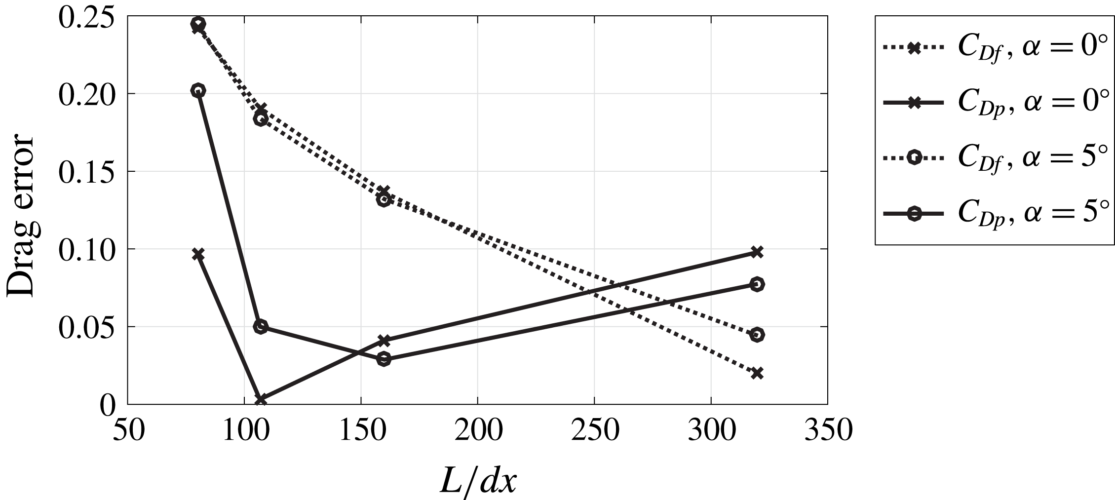
Simulations were conducted in two dimensions using the boundary data immersion method (BDIM) developed by and described in Weymouth & Yue (Reference Weymouth and Yue2011) and Maertens & Weymouth (Reference Maertens and Weymouth2015). The present method is adapted from the set-up described in Maertens et al. (Reference Maertens, Gao and Triantafyllou2017). The physical parameters of the simulation are non-dimensionalized by the fish length
 $L$
, its swimming speed
 $U_{s}=1L/s$
and the water density
 $\unicode[STIX]{x1D70C}$
. To simulate a steady swimming speed for the fish, a constant velocity inlet condition of
 $U_{\infty }=U_{s}$
is used on the left side of the fluid domain, and the fish maintains a position within the centre of the fluid domain. The Cartesian grid is uniform within a fine grid region near the fish, with
 $\text{d}x=\text{d}y=1/320$
. A
 $2\,\%$
geometric expansion ratio is used for the spacing in the far field. Validation for the numerical method used is published in Maertens et al. (Reference Maertens, Gao and Triantafyllou2017).
Two proportional-integral-derivative controllers are implemented to ensure the fish maintains its position in
 $x$
and
 $y$
; the details of these controllers are provided in § 2.4. Periodic boundary conditions are implemented on the upper and lower boundaries, and a zero gradient exit condition with global flux correction is used on the downstream (right) boundary. Simulations were conducted at
 $Re=5000$
.
2.1 Fish geometry and kinematics
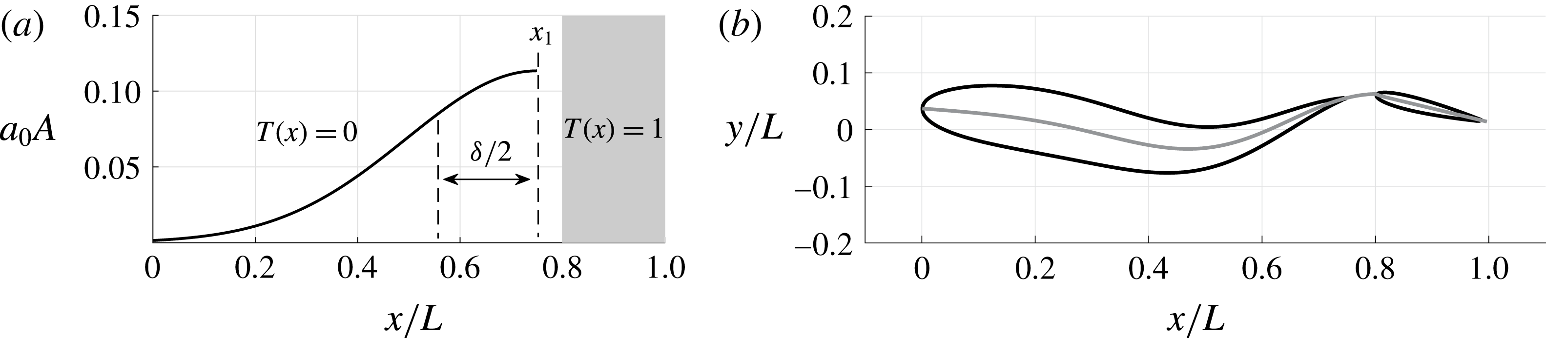
In this work, we focus on fish that use undulatory, travelling wave-based propulsion. To capture the effect of caudal fin vorticity interaction within a schooling set-up, each fish is modelled as two physically separate bodies connected by an invisible link (figure 1). This essentially captures a two-dimensional (2-D) cross-section of a fish with a narrow peduncle and high aspect ratio tail, at a slice just above the mid-height plane.
With this model, the amplitude of motion is a continuous function over the entire body, including the caudal fin, but the slope can be discontinuous at the peducle, and the tail pitching motion is allowed have an arbitrary phase with respect to the peduncle motion. This allows the tail an independent degree of freedom, but it is not fully independent of the main body. Although the two bodies are not physically connected, they are treated as if they are part of the same body with a single centre of mass, where hydrodynamic forces summed over the entire body and tail influence the translation and rotation of the centre of mass (see equations (2.10)–(2.15)).
The deformation envelope (a), and a diagram of the fish at a single time step (b). The black outline represents the total displacement of the fish, while the grey line represents the midline displacement. Note that although there is a physical gap between the body and the tail, the midline displacement is continuous between the two, creating an invisible kinematic and dynamic link.

Similar to the formulation in Maertens et al. (Reference Maertens, Gao and Triantafyllou2017), we impose a flexure on the body of the fish, parameterized by
 $5$
parameters: the frequency
 $f$
, phase
 $\unicode[STIX]{x1D719}$
and wavelength
 $\unicode[STIX]{x1D706}$
of the undulating wave, as well as two parameters (
 $x_{1}$
and
 $\unicode[STIX]{x1D6FF}$
) which govern the shape of the deformation envelope. This low-order parameterization allows us to capture the most prominent features of the swimming gait while keeping the parameter space manageable.
The fish has a total length
 $L=1$
, with a NACA0015 of chord length
 $c_{b}=0.75$
for the main body, and a NACA0012 of chord length
 $c_{t}=0.2$
for the caudal fin. The gap between the two bodies is
 $l_{g}=0.05$
. Although the caudal fin is not physically attached to the main body, the centreline extending from the head to the trailing edge is continuous, and its flexure is given by:
 $$\begin{eqnarray}\displaystyle & \displaystyle x^{\ast }(x,t)=T(x)(x_{p}+(x-x_{p}(t))\cos (\unicode[STIX]{x1D703}_{t}(t))), & \displaystyle\end{eqnarray}$$
 $$\begin{eqnarray}\displaystyle \displaystyle y^{\ast }(x,t) & = & \displaystyle a_{0}(t)(1-T(x))[A(x)\sin (2\unicode[STIX]{x03C0}(x/\unicode[STIX]{x1D706}-ft+\unicode[STIX]{x1D719}))+B(x,t)]\nonumber\\ \displaystyle & & \displaystyle +\,T(x)(y_{p}(t)+(x-x_{p}(t))\sin (\unicode[STIX]{x1D703}_{t}(t))).\end{eqnarray}$$
 $T(x)$
is the tail envelope and is defined as
 $0$
over the main body and
 $1$
over the caudal fin. This allows for the separation of the body kinematics into two sections corresponding with the undulating main body and a rigidly rotating caudal fin. While the centreline
 $y^{\ast }(x,t)$
is continuous, its slope is discontinuous at
 $x_{p}=0.78$
, a point within the gap.
The caudal fin heaves, following the trajectory at the peduncle (
 $x_{p},y_{p}(t)$
), and pitches with angle
 $\unicode[STIX]{x1D703}_{t}(t)$
, defined as:
 $$\begin{eqnarray}\displaystyle \displaystyle \unicode[STIX]{x1D703}_{t}(t) & = & \displaystyle \unicode[STIX]{x1D703}_{D}(t)+\unicode[STIX]{x1D703}_{0}(t)\sin (2\unicode[STIX]{x03C0}(x/\unicode[STIX]{x1D706}-ft+\unicode[STIX]{x1D719}+\unicode[STIX]{x1D719}_{t}))\nonumber\\ \displaystyle & & \displaystyle +\,\arctan (a_{0}(t)(b_{c}(t)\cos (2\unicode[STIX]{x03C0}ft)+b_{s}(t)\sin (2\unicode[STIX]{x03C0}ft)+d(t))).\end{eqnarray}$$
 $\unicode[STIX]{x1D703}_{D}(t)$
is a time-varying tail bias term which is calculated through a proportional-integral-derivative (PID) controller and used for steering.
 $\unicode[STIX]{x1D703}_{0}(t)$
is the nominal pitch angle, which is set to vary with the amplitude of undulation through a gain
 $k_{t}$
, such that
 $\unicode[STIX]{x1D703}_{0}(t)=k_{t}a_{0}(t)$
.
 $\unicode[STIX]{x1D719}_{t}$
is the tail pitch phase, which can be varied to adjust the phase lag between heave and pitch motion of the tail. The last term in the equation carries the angle from the hydrodynamic recoil on the body over to the tail pitch angle.
The fish body undulates with amplitude
 $a_{0}(t)$
within a Gaussian-like envelope
 $A(x)$
, defined as:
 $$\begin{eqnarray}\displaystyle & \displaystyle A(x)=\exp \left(-\!\left({\displaystyle \frac{x-x_{1}}{\unicode[STIX]{x1D6FF}}}\right)^{2}+\left({\displaystyle \frac{1-x_{1}}{\unicode[STIX]{x1D6FF}}}\right)^{2}\right). & \displaystyle\end{eqnarray}$$
Using the Gaussian envelope, the maximum flexure for the fish occurs at a point
 $x_{1}$
upstream of the trailing edge, and the width of the peak around
 $x_{1}$
is governed by
 $\unicode[STIX]{x1D6FF}$
. Physically, the point of maximum flexure occurs near the peduncle of the fish, allowing the aft portion of the fish to undergo a large displacement while retaining a low angle of attack relative to the local flow. In the study by Maertens et al. (Reference Maertens, Gao and Triantafyllou2017), it was found that such a deformation envelope was superior to a monotonically increasing flexing motion from head to tail. This suggested that the tail kinematics should not be modelled as a simple continuation of the main body kinematics, but should have an independent degree of freedom. Therefore, in the present work, we continue to use a Gaussian deformation envelope for the main body of the fish, while allowing the tail to pitch independently.
 $B(x,t)$
is the recoil term due to hydrodynamic forces on the fish:
 $$\begin{eqnarray}\displaystyle & \displaystyle B(x,t)=(a_{c}+xb_{c})\cos (2\unicode[STIX]{x03C0}ft)+(a_{s}+xb_{s})\sin (2\unicode[STIX]{x03C0}ft)+c(t)+xd(t) & \displaystyle\end{eqnarray}$$
in which
 $a_{s}$
,
 $b_{s}$
,
 $a_{c}$
,
 $b_{c}$
,
 $c(t)$
and
 $d(t)$
are calculated to ensure that linear and angular momentum are conserved as the fish undulates (equation (2.15)).
2.2 Relative timing
For two fish swimming in tandem, the timing of the upstream fish is not important to its efficiency, while the timing of the downstream fish greatly affects its swimming efficiency (Maertens et al. Reference Maertens, Gao and Triantafyllou2017). The timing of the downstream fish, which is modified through varying either the distance between the two fish or the phase of undulation, controls the interaction between the fish and the upstream wake.
To assess the importance of timing, the phase
 $\unicode[STIX]{x1D719}$
of the downstream fish is varied in this study while the distance
 $d$
between the fish is kept constant. The timing of the downstream fish is captured by the flow-relative variable
 $\unicode[STIX]{x0394}\unicode[STIX]{x1D719}$
:
 $$\begin{eqnarray}\displaystyle & \displaystyle \unicode[STIX]{x0394}\unicode[STIX]{x1D719}=\unicode[STIX]{x1D719}-\unicode[STIX]{x1D719}_{1}, & \displaystyle\end{eqnarray}$$
 $$\begin{eqnarray}\displaystyle & \displaystyle \unicode[STIX]{x1D719}_{1}=d/\unicode[STIX]{x1D706}_{w}+\unicode[STIX]{x1D719}_{w}. & \displaystyle\end{eqnarray}$$
 $\unicode[STIX]{x0394}\unicode[STIX]{x1D719}$
provides the phase relationship between the motion of the nose of the downstream fish and the wake of the upstream fish, which has phase
 $\unicode[STIX]{x1D719}_{w}$
and wavelength
 $\unicode[STIX]{x1D706}_{w}$
.
 $\unicode[STIX]{x1D719}_{1}$
is the phase of the wake at the nose of the downstream fish.
2.3 Dynamics for self-propelled swimming
While the kinematics described above govern the flexure of the fish, the total displacement results from the centre of mass motion as well as the instantaneous deformation. We define a self-propelled fish as one for which the hydrodynamic forces created by the interaction between the fish and the surrounding flow alone govern the centre of mass motion; the fish is not held in place or otherwise restrained unless the steady-state force in the direction of restraint is negligible, as described in § 2.4.
The fluid is governed by the Navier–Stokes equations, which are non-dimensionalized by the fish body length
 $L$
, the average swimming speed
 $U_{s}$
and the density of water
 $\unicode[STIX]{x1D70C}$
:
 $$\begin{eqnarray}\displaystyle & \displaystyle {\displaystyle \frac{\unicode[STIX]{x2202}\boldsymbol{u}}{\unicode[STIX]{x2202}t}}=-(\boldsymbol{u}\boldsymbol{\cdot }\unicode[STIX]{x1D735})\boldsymbol{u}+{\displaystyle \frac{1}{Re}}\unicode[STIX]{x1D6FB}^{2}\boldsymbol{u}-\unicode[STIX]{x1D735}p, & \displaystyle\end{eqnarray}$$
 $$\begin{eqnarray}\displaystyle & \displaystyle \unicode[STIX]{x1D735}\boldsymbol{\cdot }\boldsymbol{u}=0, & \displaystyle\end{eqnarray}$$
where
 $\boldsymbol{u}$
is the fluid velocity normalized by
 $U_{s}$
, the pressure
 $p$
is normalized by
 $\unicode[STIX]{x1D70C}U_{s}^{2}$
and
 $Re=U_{s}L/\unicode[STIX]{x1D708}$
is the Reynolds number, where
 $\unicode[STIX]{x1D708}$
is the kinematic viscosity of the fluid.
In a reference frame moving with the fish at velocity
 $U_{s}$
, the motion of the fish is the superposition of the prescribed flexure and a rigid body motion. The rigid body motion is defined by the translation and rotation of the centre of mass, effected by the net hydrodynamic force
 $F_{h}$
on the body:
 $$\begin{eqnarray}\displaystyle & \displaystyle \boldsymbol{F}_{h}=\oint _{\unicode[STIX]{x1D6FA}_{b}}\boldsymbol{f}_{h}\,\text{d}s, & \displaystyle\end{eqnarray}$$
where
 $\unicode[STIX]{x1D6FA}_{b}$
is the surface of the body. The moment about the centre of mass, caused by hydrodynamic forces is:
 $$\begin{eqnarray}\displaystyle & \displaystyle \boldsymbol{M}_{h}=\oint _{\unicode[STIX]{x1D6FA}_{b}}\boldsymbol{x}^{\ast }\times \boldsymbol{f}_{h}\,\text{d}s, & \displaystyle\end{eqnarray}$$
where
 $\boldsymbol{x}^{\ast }$
is the distance vector to a point on the surface of the body, in the local frame attached to the fish centre of mass.
Then, the motion of the centre of mass is given by Newton’s law:
 $$\begin{eqnarray}\displaystyle & \displaystyle {\displaystyle \frac{\text{d}}{\text{d}t}}(\unicode[STIX]{x1D648}\boldsymbol{V})=\boldsymbol{F}_{h}. & \displaystyle\end{eqnarray}$$
In two dimensions, the variables are:
 $$\begin{eqnarray}\displaystyle & \displaystyle \boldsymbol{X}=\left(\begin{array}{@{}c@{}}x_{c}\\ y_{c}\\ \unicode[STIX]{x1D703}\end{array}\right),\quad \boldsymbol{V}=\left(\begin{array}{@{}c@{}}v_{c}^{x}\\[3.0pt] v_{c}^{y}\\ \unicode[STIX]{x1D714}_{b}\end{array}\right),\quad \boldsymbol{F}_{h}=\left(\begin{array}{@{}c@{}}F_{h}^{x}\\[4.0pt] F_{h}^{y}\\[3.0pt] M_{c}^{z}\end{array}\right),\quad \unicode[STIX]{x1D648}=\left(\begin{array}{@{}ccc@{}}m & 0 & 0\\ 0 & m & 0\\ 0 & 0 & I_{c}\end{array}\right), & \displaystyle\end{eqnarray}$$
 $\unicode[STIX]{x1D648}$
is the mass matrix, in which
 $m$
is the mass of the body and
 $I_{c}$
is its moment of inertia with respect to the centre of mass.
The total velocity of a point on the surface of the fish is the superposition of the centre of mass velocity
 $\boldsymbol{v}_{c}$
, the prescribed flexing velocity
 $\boldsymbol{v}^{\ast }$
and the rigid body rotation:
 $$\begin{eqnarray}\displaystyle & \displaystyle \boldsymbol{v}=\boldsymbol{v}_{c}+\boldsymbol{v}^{\ast }+\unicode[STIX]{x1D74E}_{b}\times \boldsymbol{x}^{\ast }. & \displaystyle\end{eqnarray}$$
The prescribed flexing motion must also conserve linear and angular momentum:
 $$\begin{eqnarray}\displaystyle & \displaystyle {\displaystyle \frac{\text{d}}{\text{d}t}}\int _{\unicode[STIX]{x1D6FA}_{b}}\unicode[STIX]{x1D70C}\boldsymbol{v}^{\ast }\,\text{d}\unicode[STIX]{x1D6FA}_{b}=0, & \displaystyle\end{eqnarray}$$
 $$\begin{eqnarray}\displaystyle & \displaystyle {\displaystyle \frac{\text{d}}{\text{d}t}}\int _{\unicode[STIX]{x1D6FA}_{b}}\unicode[STIX]{x1D70C}\boldsymbol{v}^{\ast }\times \boldsymbol{x}^{\ast }\,\text{d}\unicode[STIX]{x1D6FA}_{b}=0. & \displaystyle\end{eqnarray}$$
This gives rise to the terms
 $a_{s}$
,
 $b_{s}$
,
 $a_{c}$
,
 $b_{c}$
,
 $c(t)$
and
 $d(t)$
in (2.5).
2.4 PID controllers to ensure self-propulsion and straight line motion
Two proportional-integral-derivative (PID) controllers are implemented: the first adjusts the thrust by tuning the amplitude of the swimming gait
 $a_{0}(t)$
, and the second steers the fish by adjusting the tail pitch bias
 $\unicode[STIX]{x1D703}_{D}(t)$
. As a result, these two controllers alter the flexing kinematics of both fish to ensure that each propels itself at a constant velocity and swims in a straight line. After the PID parameters converge to a steady state, the hydrodynamics over each swimming period also converge to a steady state, which greatly simplifies the analysis to be performed. For a fish swimming in line with another fish, the vortices shed over several periods affect the swimming efficiency; therefore, for a steady-state analysis, it is important for the vortices shed by both fish to be consistent over multiple swimming periods.
For a self-propelled fish, the time-averaged linear momentum in
 $x$
is used as feedback for the first controller, and the time-averaged linear momentum in
 $y$
is used as feedback for the second controller. As a result, the PID controller drives the average force in both directions to zero, so that the fish maintains a constant swimming velocity and does not drift to either side. Analysis on each case is performed after the simulation has reached convergence for 5–10 swimming cycles.
To further improve the convergence times without significantly affecting the results, it is possible to fix the fish in
 $x$
(Maertens et al.
Reference Maertens, Gao and Triantafyllou2017). In this case, the fish is not self-propelled at the start of the simulation while the PID parameters are converging, but it becomes self-propelled after the simulation reaches a steady state. Maertens et al. (Reference Maertens, Gao and Triantafyllou2017) demonstrated that the average power coefficient and self-propelled swimming amplitude vary by less than
 $1\,\%$
for a fish fixed in
 $x$
compared with a fish free to move in both directions. This result corroborates the finding by Bale et al. (Reference Bale, Hao, Bhalla and Patankar2014) that the power consumed in streamwise oscillations
 $\overline{P}_{osc}=\overline{F_{x}u^{\prime }}$
, is negligible compared with the net power consumed. The streamwise oscillations, likewise, are small compared with the overall swimming velocity. For this case, the time-averaged drag is used as feedback for the first controller, to ensure that drag (and thrust) are zero when the simulation has converged, so that the fish self-propels at constant velocity.
The controllers act on the time-averaged error, and for the momentum this is:
 $$\begin{eqnarray}\displaystyle & \displaystyle \boldsymbol{e}_{k}=f\mathop{\sum }_{i=k_{0}}^{k-1}m\boldsymbol{v}_{i}(t_{i+1}-t_{i}), & \displaystyle\end{eqnarray}$$
where
 $k_{0}$
is the index corresponding to the time step exactly one period before. The time-averaged drag is similar.
The integral of the error is:
 $$\begin{eqnarray}\displaystyle & \displaystyle \boldsymbol{e}_{i,k}=\mathop{\sum }_{i=0}^{k-1}\boldsymbol{e}_{i}(t_{i+1}-t_{i}). & \displaystyle\end{eqnarray}$$
And the derivative of the error is:
 $$\begin{eqnarray}\displaystyle & \displaystyle \boldsymbol{e}_{d,k}={\displaystyle \frac{\boldsymbol{e}_{k}-\boldsymbol{e}_{k-1}}{t_{k}-t_{k-1}}}. & \displaystyle\end{eqnarray}$$
A window smoothing filter is applied to each error term to improve stability. At the beginning of each time step,
 $a_{0,k}$
and
 $\unicode[STIX]{x1D703}_{D,k}$
are adjusted as follows:
 $$\begin{eqnarray}\displaystyle & \displaystyle a_{0,k}=\max (a_{0,k-1}+(t_{k}-t_{k-1})(K_{p}^{x}e_{k}^{x}+K_{i}^{x}e_{i,k}^{x}+K_{d}^{x}e_{d,k}^{x}),0), & \displaystyle\end{eqnarray}$$
 $$\begin{eqnarray}\displaystyle & \displaystyle \unicode[STIX]{x1D703}_{D,k}=-(K_{p}^{y}e_{k}^{y}+K_{i}^{x}ye_{i,k}^{y}+K_{d}^{y}e_{d,k}^{y}). & \displaystyle\end{eqnarray}$$
Where
 $e^{x}$
and
 $e^{y}$
denote the error terms in
 $x$
or
 $y$
. The gain coefficients used were:
 $$\begin{eqnarray}\displaystyle \left.\begin{array}{@{}l@{}}\text{for force control in }x\text{:}\quad K_{p}^{x}=5,\quad K_{i}^{x}=5,\quad K_{d}^{x}=0.1,\\ \text{for displacement control in }x\text{:}\quad K_{p}^{x}=10,\quad K_{i}^{x}=0.1,\quad K_{d}^{x}=1,\\ \text{for displacement control in }y\text{:}\quad K_{p}^{y}=30,\quad K_{i}^{y}=30,\quad K_{d}^{y}=10.\end{array}\right\} & & \displaystyle\end{eqnarray}$$
2.5 Performance metrics
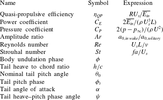
To compare the performance of each fish, we use the quasi-propulsive efficiency defined in Maertens et al. (Reference Maertens, Gao and Triantafyllou2017):
 $$\begin{eqnarray}\displaystyle & \displaystyle \unicode[STIX]{x1D702}_{QP}={\displaystyle \frac{RU_{s}}{\overline{E_{in}}}}. & \displaystyle\end{eqnarray}$$
 $R$
is the resistance of the rigid–straight body towed at constant speed, and
 $\overline{E_{in}}$
is the period-averaged power consumed to undulate the body. As discussed in Maertens, Triantafyllou & Yue (Reference Maertens, Triantafyllou and Yue2015), the quasi-propulsive efficiency is an intuitive, non-dimensional performance metric, which is used extensively in naval architecture to define efficiency of propulsion of marine vehicles. For simplicity, this term is used interchangeably with ‘efficiency’ throughout this paper.
Since inefficiencies in the leader’s gait are in general advantageous to the follower, it is also useful to consider the efficiency of the two-fish system, defined as:
 $$\begin{eqnarray}\displaystyle & \displaystyle \unicode[STIX]{x1D702}_{QP,sys}={\displaystyle \frac{R_{l}U_{s,l}+R_{f}U_{s,f}}{\overline{P_{l,in}}+\overline{P_{f,in}}}}, & \displaystyle\end{eqnarray}$$
where
 $R_{l}$
,
 $U_{s,l}$
and
 $\overline{P_{l,in}}$
denote the resistance, swimming speed and period-averaged power consumed by the leader, and
 $R_{f}$
,
 $U_{s,f}$
and
 $\overline{P_{f,in}}$
denote the resistance, swimming speed and period-averaged power consumed by the follower.
In addition to the efficiency, the thrust generated and power consumed along the body of the fish are used extensively throughout this study to draw conclusions on the effect of individual vortex interactions. The thrust created by the local pressure
 $p_{i}$
along a discrete section
 $s_{i}$
can be calculated by multiplying the local pressure by the component of the normal vector in the forward
 $x$
direction:
 $T_{i}=p_{i}n_{i}^{x}$
. The power consumed through interaction with the local hydrodynamic force is
 $E_{i}=-\boldsymbol{F}_{h,i}\boldsymbol{\cdot }v_{i}$
.
Over the entire body of the fish, we define the power coefficient
 $C_{E}$
as:
 $$\begin{eqnarray}\displaystyle & \displaystyle C_{E}={\displaystyle \frac{\overline{E_{in}}}{1/2\unicode[STIX]{x1D70C}U_{s}^{3}L}}. & \displaystyle\end{eqnarray}$$
And the thrust coefficient
 $C_{T}$
as:
 $$\begin{eqnarray}\displaystyle & \displaystyle C_{T}={\displaystyle \frac{\overline{T}}{1/2\unicode[STIX]{x1D70C}U_{s}^{2}L}}. & \displaystyle\end{eqnarray}$$
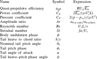
Additional relevant parameters are defined in table 1.
Kinematic and other dimensionless parameters.
3 Hydrodynamic interactions and timing with an independent caudal fin
Fast swimming fish and mammals, such as tunas and dolphins have developed a very narrow peduncle just ahead of their caudal fin, allowing their tails to be actuated in angular (pitching) motion that can be largely independent of the phasing of the peduncle lateral (heaving) motion. While the need for a narrowing of the peduncle is related to minimizing the recoil (Lighthill Reference Lighthill1975), it also facilitates the independent pitching of the caudal fin, which is not as flexible for these fast swimmers as for smaller fish. A tail that can be controlled independently can effect vorticity control which is crucial in flow control and energy recovery. The structure of the penducular keel of tunas is particularly striking, because the tendons which transmit force from the body musculature to the caudal fin follow the outer contour of the bony peduncular keel. Fierstine & Walters (Reference Fierstine and Walters1968) proposed that in doing so, the peduncular keel acts as a pulley for the great lateral tendons which transmit force from the muscle mass within the body to the rays of the caudal fin, substantially increasing the torque applied to the fin rays for powerful and precise control. Likewise, in the design of the RoboTuna, it was essential to fit a large pulley at the last link of the robot, just ahead of the tail, in order to create the requisite large moments (Sachinis Reference Sachinis2000). The optimal kinematics involved a tail motion with distinct phasing from the body motion.
In the present study, the goal is to study the potential gain from allowing the caudal fin of a simulated fish to pitch independently from the main body. Note that while the caudal fin is allowed this additional degree of freedom, it is not fully independent but is kinematically and dynamically bound to the main body (see § 2.3). To simplify the analysis, we model the caudal fin, which is physically separate from the body, as a rigid NACA0015 airfoil. This provides the ability for the tail to manipulate and generate vorticity, without involving the complexity of parameterizing a flexible caudal fin. In fact, the tails and fins of many underwater animals closely resemble high aspect ratio foils, so numerous researchers have used rigid NACA foils to model fish dorsal and/or caudal fins (Zhu et al. Reference Zhu, Wolfgang, Yue and Triantafyllou2002; Triantafyllou, Techet & Hover Reference Triantafyllou, Techet and Hover2004; Lauder et al. Reference Lauder, Anderson, Tangorra and Madden2007; Melli & Rowley Reference Melli and Rowley2010), as well as fins on other animals (Licht et al. Reference Licht, Wibawa, Hover and Triantafyllou2010; Izraelevitz & Triantafyllou Reference Izraelevitz and Triantafyllou2014). Due to the narrow caudal peduncle discussed above, modelling the caudal fin as a separate body replicates a 2-D cross-section of the fish just above the peduncle. While there are some three-dimensional effects that cannot be captured in two dimensions, such as the spanwise evolution of the leading edge vortex on caudal fins (Borazjani & Daghooghi Reference Borazjani and Daghooghi2013), many two-dimensional effects do carry over to three dimensions (Maertens et al. Reference Maertens, Gao and Triantafyllou2017), and provide considerable insight on the physics behind the main hydrodynamic interactions.
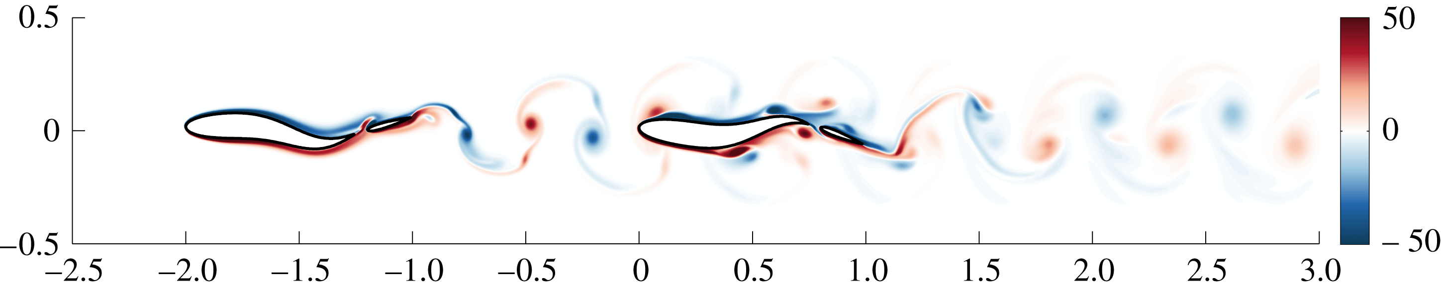
A snapshot of the vorticity field when a fish modelled with a distinct caudal fin swims at a distance of one body length directly behind another fish.
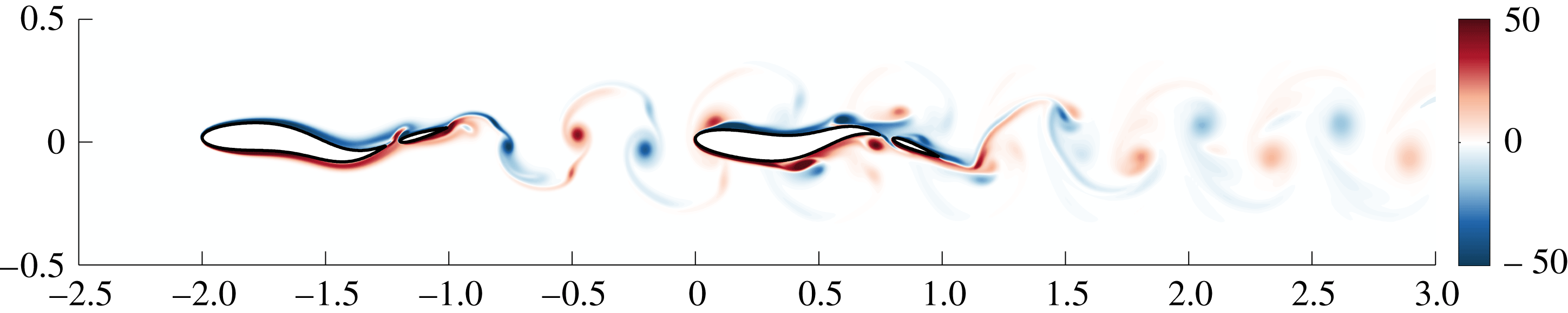
Presently, the tail pitch phase is constrained to be within a range of approximately
 $70^{\circ }$
for thrust-producing configurations. However, we will demonstrate that small phase changes within this range result in large changes in the swimming efficiency. A large body of research shows that the motion profile of the caudal fin strongly affects its performance (Gopalkrishnan et al.
Reference Gopalkrishnan, Triantafyllou, Triantafyllou and Barrett1994; Hover, Haugsdal & Triantafyllou Reference Hover, Haugsdal and Triantafyllou2004; Triantafyllou et al.
Reference Triantafyllou, Techet and Hover2004; Schouveiler, Hover & Triantafyllou Reference Schouveiler, Hover and Triantafyllou2005). Observations from fish show the same trend; as discussed, tunas have precise control over an independently pitching caudal fin (Fierstine & Walters Reference Fierstine and Walters1968), allowing them to achieve optimal swimming configurations under many different conditions.
3.1 Effect of an independently pitching tail
A pitching rigid tail can alter the wake signature by changing the pitching amplitude
 $\unicode[STIX]{x1D703}_{0}$
, and the tail phase angle
 $\unicode[STIX]{x1D719}_{t}$
.
 $\unicode[STIX]{x1D719}_{t}$
is the phase angle of the tail and one must subtract the phase angle of the peduncle in order to find the relative phase angle between peduncle and caudal fin,
 $\unicode[STIX]{x1D713}$
.
Results from harmonic flapping foils show that the Strouhal number, variation in phase lag between heave and pitch, the heave amplitude to chord ratio and the heave and pitch amplitudes can result in a wide variety of wake topologies for flapping foils (Anderson et al. Reference Anderson, Streitlien, Barrett and Triantafyllou1998; Lentink et al. Reference Lentink, Muijres, Donker-Duyvis and van Leeuwen2008; Schnipper, Andersen & Bohr Reference Schnipper, Andersen and Bohr2009; Koochesfahani Reference Koochesfahani1989). A variable of great importance is the angle of attack and its profile as a function of time, which greatly impacts wake topology (Read, Hover & Triantafyllou Reference Read, Hover and Triantafyllou2003; Hover et al. Reference Hover, Haugsdal and Triantafyllou2004).
While the present study corroborates these findings, the set-up is distinct due to the self-propelled nature of the fish. Since the caudal fin is kinematically and dynamically bound to the main body, it cannot be treated as a fully controllable airfoil placed to control the vorticity shed upstream. Parameters such as the phase lag between heave and pitch motion, the Strouhal number and the angle of attack cannot be controlled in open loop. With a self-propelled set-up, the heave profile for the caudal fin equals the displacement at the peduncle
 $y_{p}(t)$
, and cannot be directly controlled, because it is a complex function of the prescribed deformation, the amplitude of undulation, and the hydrodynamic recoil and is, in general, not harmonic. Therefore, rather than controlling the set of parameters traditionally used with flapping foils, we vary the amplitude and phase of the tail pitch in optimizing the motion of the tail. As these parameters affect the hydrodynamics of the fish, the parameters traditionally considered in flapping foil studies also vary, and will be presented for comparison.
3.2 Optimization of body and tail pitch phase for tandem swimming
Simulations were conducted in which two fish with distinct caudal fins swim in tandem, with the follower fish at one body length downstream from the leader. The leader fish employs an optimized gait with a tail phase of
 $\unicode[STIX]{x1D719}_{t}=0.25$
, which produces a clean reverse Kármán street. The leader’s inefficiency is in general to the follower’s advantage, but by choosing an efficient mode, we minimize this effect. The body phase and the tail phase of the follower fish were varied for optimization.
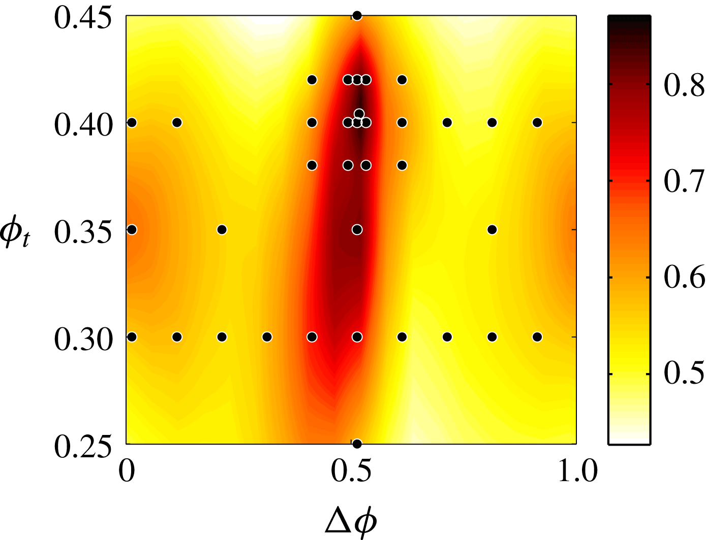
The optimization (figure 3) shows that while the quasi-propulsive efficiency for the downstream fish varies by only around 10 % over the majority of the parameter space, within a very narrow parametric range centred around
 $\unicode[STIX]{x0394}\unicode[STIX]{x1D719}=0.51$
and
 $\unicode[STIX]{x1D719}_{t}=0.4$
, the efficiency reaches a remarkable
 $\unicode[STIX]{x1D702}_{QP}=90\,\%$
. At this configuration, the follower fish swims with roughly half the energy required to swim alone.
The swimming efficiency of the downstream fish, modelled with an independently pitching tail, as a function of the wake-relative phase difference
 $\unicode[STIX]{x0394}\unicode[STIX]{x1D719}$
and the tail pitch phase
 $\unicode[STIX]{x1D719}_{t}$
. The black dots represent individual simulation results, and the contour plot is created using a thin-plate smoothing spline with smoothing parameter
 $p=0.999$
.
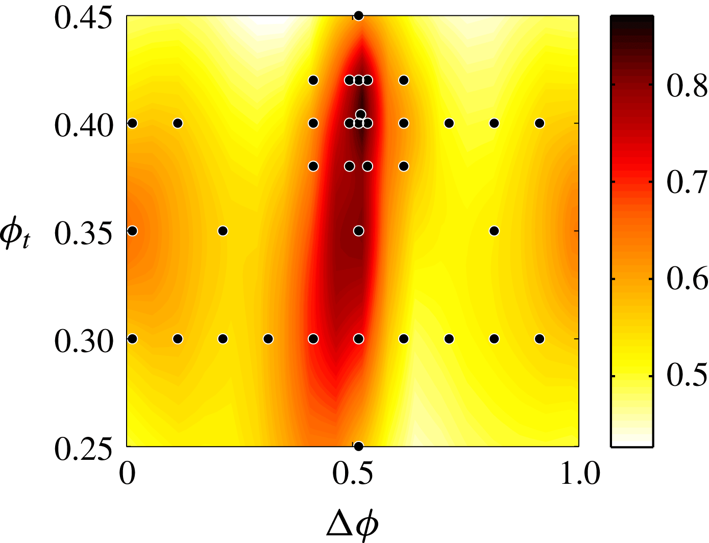
In fact, over the majority of the parameter space, the variation in efficiency is very similar to the variation of efficiency for a fish modelled without a distinct caudal fin, reported in Maertens et al. (Reference Maertens, Gao and Triantafyllou2017). The fish experiences a reduced drag and increased efficiency for roughly half of the possible phase differences
 $\unicode[STIX]{x0394}\unicode[STIX]{x1D719}$
, and an increased drag and decreased efficiency for the other half, with a range of around
 $\unicode[STIX]{x0394}\unicode[STIX]{x1D702}_{QP}=10\,\%$
. However, with the ability to independently time the tail, a 50 % increase in efficiency for the follower fish is possible. At the optimal configuration, the efficiency of the two-fish system increases by over 15 %, from
 $\unicode[STIX]{x1D702}_{QP,sys}=40\,\%$
to 55.8 %.
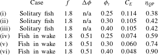
Near the optimal efficiency, proper timing of the body phase and the tail pitch phase are important. Although a solitary fish swims optimally with
 $\unicode[STIX]{x1D719}_{t}\approx 0.36$
, the optimal tail pitch phase within the wake in this case is
 $\unicode[STIX]{x1D719}_{t}=0.4$
. When swimming alone, altering the tail phase between the feasible range of
 $0.25\leqslant \unicode[STIX]{x1D719}_{t}\leqslant 0.45$
results in an efficiency variation of only approximately 5 %. However, in the wake of the upstream fish, adjusting the tail phase across the same range can change the efficiency by over 30 %. This demonstrates that independent control of the tail pitch can greatly improve swimming performance in the presence of vortices; this independent control allows for fine vorticity control around the caudal peduncle and tail, which will be shown in detail within the next section.
3.3 Energy recovery through vorticity control
For the optimal configuration of
 $\unicode[STIX]{x0394}\unicode[STIX]{x1D719}=0.51,\unicode[STIX]{x1D719}_{t}=0.4$
, the fish swims with an efficiency of
 $\unicode[STIX]{x1D702}_{QP}=90\,\%$
. This timing depends on the exact configuration of both fish, as it arises from hydrodynamic interactions along the entire body. For instance, the shape and kinematics of each fish affect the spacing between vortices, which can result in an increased or decreased ability of the following fish to take advantage of all vortices simultaneously (at a given phase difference). However, while the optimal phase difference may vary according to the exact swimming configuration of the fish, local hydrodynamic interactions remain consistent between the optimal phasing at different configurations, and are highly detectable. Therefore, we will discuss in this section the physical mechanisms that were found to be associated with the large gains in efficiency.
Efficiency depends on the control of vorticity along the entire body. Near the head, the fish significantly increases the thrust generated by slaloming among oncoming vortices. Along the body, some energy is lost, but by ensuring a proper phasing that keeps the induced vortices close to the peak of the undulation crests, the energy loss is relatively small. By balancing timing at the nose and timing along the body in this manner, the fish can maximize energy savings at the nose while minimizing energy loss along the body. This proper timing of interactions at the nose and along the body are important, but in this case, well-coordinated interactions at the peduncle and tail give rise to the most significant energy savings.
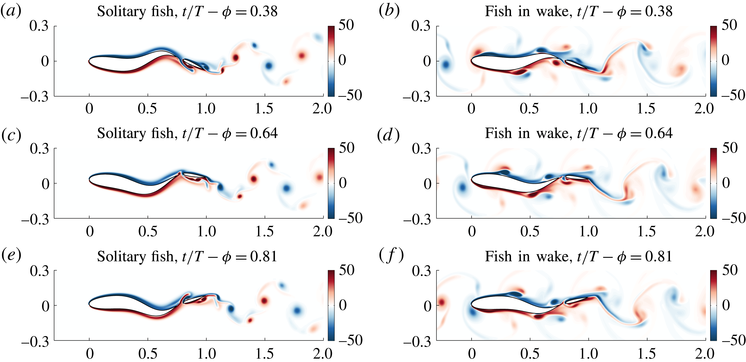
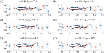
Figure 4 depicts three consecutive snapshots of the fish swimming alone (a,c,e), and the fish swimming with optimal phase within the wake of an upstream fish (b,d,f). The time step of each snapshot is denoted as
 $t/T-\unicode[STIX]{x1D719}$
modulo (mod) 1, because after steady state is reached, the fish kinematics and flow field within each swimming period is identical.
Snapshots of the vorticity field for a solitary fish (a,c,e) and a well-coordinated fish within the wake of an upstream fish (b,d,f), for consecutive time steps (mod 1). The interaction with the upstream wake greatly modifies the downstream wake, as well as the flow around the peduncle.
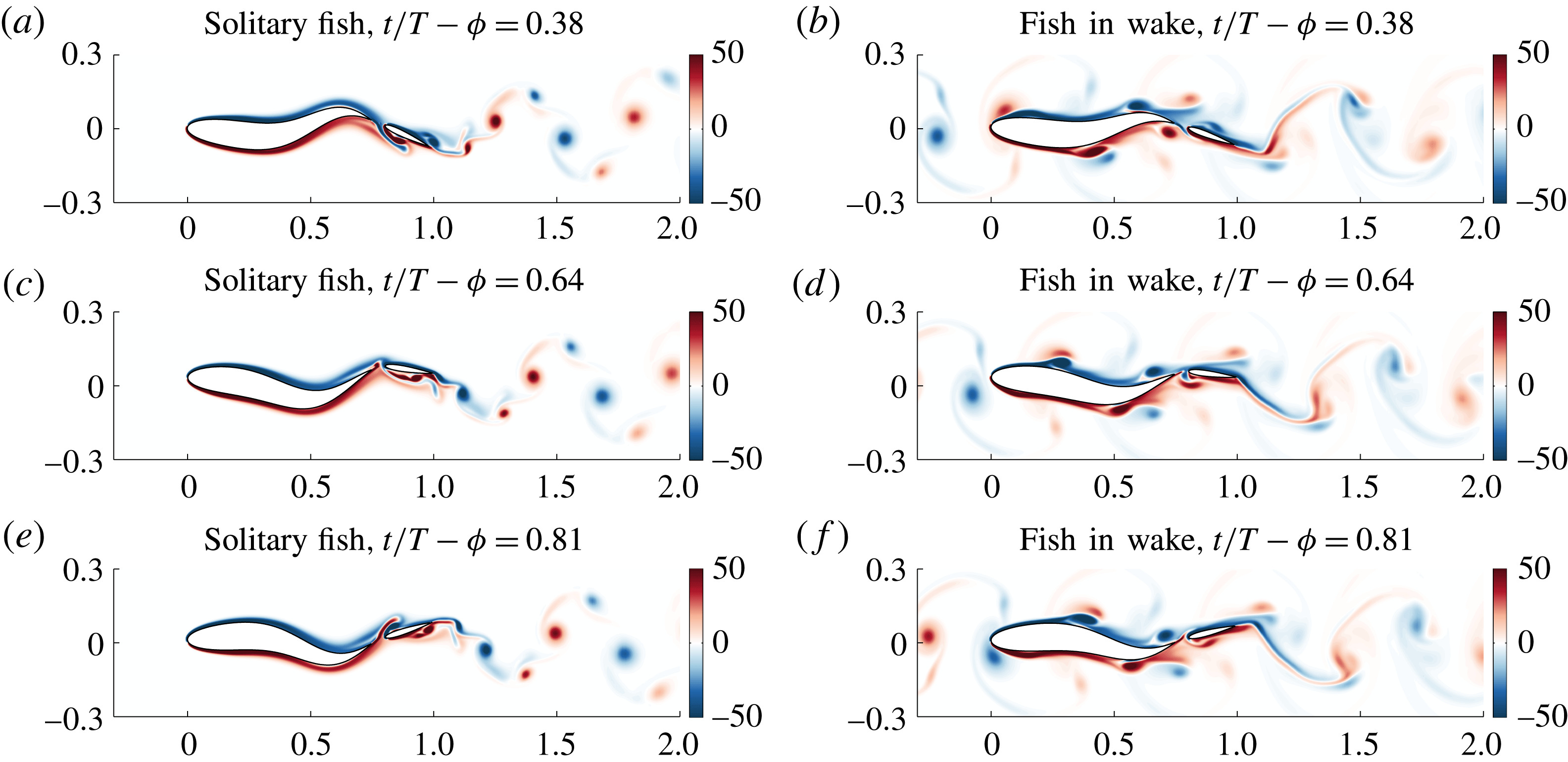
Notably, in figure 4(a), leading edge vortex shedding on the caudal fin is accompanied by a small jet through the peduncle region. Simultaneously, the leading edge vortex from the previous half-cycle on the right has just reached the trailing edge of the caudal fin. In figure 4(c), the leading edge vortex on the right has just shed. In figure 4(e), a smaller trailing edge vortex is shed from the right side of the caudal fin, while the leading edge vortex on the left approaches the trailing edge. A small jet forms at the penduncle, directed toward the right.
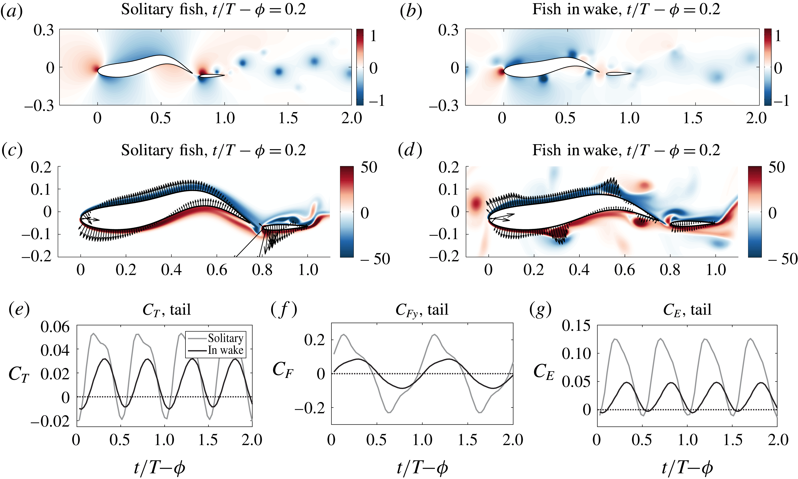
Snapshots of the pressure field for (a) a solitary fish and (b) a well-coordinated fish within the wake of an upstream fish. (c,d) The local pressure force on the surface of the fish body, plotted over a snapshot of the vorticity field. The high pressures around the leading edge of the caudal fin for the solitary fish have been greatly reduced for the fish within the wake, resulting in (e) nearly the same thrust generation with (f) decreased lateral force magnitudes and (g) greatly reduced power consumption.

In contrast, figures 4(b), 4(d) and 4(f) do not depict a jet forming through the peduncle region at all. In fact, as the positively signed induced vortex approaches from upstream (on the left), it changes the nature of the flow around the caudal fin such that leading edge vortex formation is nearly suppressed. Although a small jet forms through the gap in figure 4(d), the negative vorticity annihilates with the passing induced vortex to weaken both. The remaining positive vortex is significantly weakened and sheds with the positive trailing edge vortex during the following half-cycle. Due to the suppressed vortex shedding and the annihilation of upstream vorticity, the wake signature of the downstream fish is significantly reduced, resulting in increased swimming efficiency. In fact, in comparing this fish (b,d,f) with its solitary counterpart (a,c,e), the row of vortices near the centre of the wake have completely disappeared, leaving only the weaker set of vortices on the outside of the wake. This result, following that by Gopalkrishnan et al. (Reference Gopalkrishnan, Triantafyllou, Triantafyllou and Barrett1994), demonstrates that increased efficiency is associated with the formation of a weakened vortex wake, which is indicative of energy extraction by the fish from the upstream vortices.
To further illustrate how this vorticity control affects the swimming efficiency, a snapshot of the pressure field for both the solitary fish and the fish within the wake are shown in figures 5(a) and 5(b), respectively. As the negative induced vortex on the right passes over the peduncle region, and a positive induced vortex approaches the peduncle region on the left, they work together to oppose and reduce the relative velocity due to the transverse motion of the caudal fin. This causes a significant reduction in the pressure gradient around the caudal fin (compare figures 5 a and 5 b), and the instantaneous lateral pressure force (compare figures 5 c and 5 d).
Over a full swimming cycle, this does not significantly reduce the mean thrust force, but greatly reduces the magnitude of oscillations in the thrust and lift forces experienced by the caudal fin to reduce the overall power consumption (figure 5 e–g). Increased amplitude of oscillations in the forces is typically detrimental because it results in larger oscillations in the acceleration and therefore velocity. These fluctuations in the motion increase power consumption with no benefit, and therefore reduce efficiency (Bale et al. Reference Bale, Hao, Bhalla and Patankar2014).
Furthermore, energy is extracted through two additional mechanisms near the tail. First, as the induced vortex approaches the caudal fin, its thrust coefficient is amplified due to its increased slope, taking advantage of the low pressure core of the vortex. Secondly, as the vortex from the original upstream wake passes the trailing edge of the downstream fish (figure 4 f), it pairs up with and annihilates an oppositely signed vortex shed by the downstream fish to further reduce the downstream wake signature.
This combination of events, from the balance of timing between the nose and the body, to the transfer of energy at the caudal peduncle and tail of the fish, contribute to the greatly increased efficiency of this fish. Ultimately, it is clear that the wake signature for the fish within the wake (figure 4 b,d,f) is significantly weaker than both the wake of the upstream fish, and the wake shed by the fish swimming solitarily (figure 4 a,c,d). This is a clear indication that energy has been extracted from the wake in a beneficial manner, which is supported by the radically increased efficiency of the fish.
While the use of vorticity generated along the body to enhance performance is limited in high performance swimmers, which are already highly optimized, Fish (Reference Fish2010) hinted at the potential for large energy gains through the control of vortices generated by energy sources external to the fish (such as when schooling). Presently, we demonstrated that indeed, vorticity generated upstream can be exploited to improve the swimming efficiency of a schooling fish far beyond what could be achieved for a solitary fish. Self-propulsion is always associated with some energy loss. Execution of the swimming motions necessary for forward motion results in vorticity convected into the wake, which is essentially wasted energy (Videler Reference Videler1993; Fish Reference Fish2010). Figures 4 and 5 show that in this case, the downstream fish can execute vorticity control to dramatically reduce the lateral forces and loss in efficiency associated with the undulation of the rigid caudal fin. Hence, we use energy recovery to describe this; the downstream fish is able to recover a large portion of the energy required to swim in quiescent water, by reducing the energy loss mechanisms associated with its undulating motions. While the fish is able to recover some of the energy lost due to its necessary swimming motions simply by being in the wake of another fish, proper timing allows it to recover far more energy through thrust augmentation and vorticity annihilation.
3.4 Sensitivity to timing
The results of the previous section and figure 3 show that timing of motion is critical for the downstream fish. The annihilation of vorticity at the peduncle and in the wake of the fish depends on the precise phase relation to both the wake vortices originating from the upstream fish as well as the induced vortices emanating from the body of the following fish.
In order to demonstrate the precise interactions that give rise to the dramatically increased efficiency at
 $\unicode[STIX]{x0394}\unicode[STIX]{x1D719}=0.51,\unicode[STIX]{x1D719}_{t}=0.4$
, we will show results for fish swimming at small deviations from the optimal body phase and tail phase.
The swimming performance is extremely sensitive to the timing of both the body undulation phase and the tail pitch phase; a change of 0.1 (
 $36^{\circ }$
) in either phase can result in a change of over 15 % in efficiency. While this may be expected for the body undulation phase, which affects the timing of the entire body relative to the surrounding vortices (figure 6
a), it is surprising that relatively small changes in the tail pitch motion, which affects the timing of only the tail (figure 6
b), results in such large efficiency changes as well.
Illustration of the kinematic changes resulting from small variations in the (a) body phase
 $\unicode[STIX]{x1D719}$
, and (b) tail pitch phase
 $\unicode[STIX]{x1D719}_{t}$
. While changes to the body phase affect the timing of the entire body relative to surrounding vortices, changes to the tail phase affect only the timing at the tail.

Snapshots of the vorticity field at
 $t/T-\unicode[STIX]{x1D719}=0,0.125,0.25,0.375$
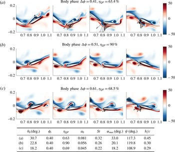
(left to right, mod 1) for fish with varying body phase. The arrows plotted over the bodies represent the local pressure force observed at the surface of the fish. When the timing is varied from the optimal point of (b)
 $\unicode[STIX]{x0394}\unicode[STIX]{x1D719}=0.51$
, the interaction between the peduncle and the approaching negative induced vortex (on the right) is changed. As a result, the jet and leading edge vortex shedding is not suppressed when the vortex arrives (a) slightly later or (c) slightly earlier, resulting in larger lateral pressure force magnitudes. The variables used in the table are defined in table 1.

3.4.1 Why efficiency is reduced away from optimal phasing
As shown, the quasi-propulsive efficiency is around 50–60 % over the majority of the parameter space spanning
 $\unicode[STIX]{x0394}\unicode[STIX]{x1D719}$
and
 $\unicode[STIX]{x1D719}_{t}$
. For
 $\unicode[STIX]{x0394}\unicode[STIX]{x1D719}=0.41$
, the efficiency is
 $\unicode[STIX]{x1D702}_{QP}=63\,\%$
. As shown in figure 7(a), at this phase the induced vortex does not suppress the leading edge vortex shedding at the caudal fin but, instead, enhances it. As the induced vortex arrives slightly later, it reaches the peduncle just as the caudal fin leading edge reaches its maximum displacement to the left and begins to move toward the right. As a result, the induced vortex is pulled through the gap, causing stronger leading edge vortex formation and a messier and more intense wake. This unnecessary vortex shedding results in large instantaneous lateral forces on the caudal fin, as shown. Although this fish still swims more efficiently than a solitary fish, with
 $\unicode[STIX]{x1D702}_{QP}=63.4\,\%$
, it does not harness the energy of the induced vortex optimally.
Similarly, for
 $\unicode[STIX]{x0394}\unicode[STIX]{x1D719}=0.61$
, the induced vortex does not suppress the flow through the peduncle region. In this case, the vortex arrives slightly early, as the leading edge of the caudal fin is just beginning to move away (figure 7
c). As a result, the vortex is already above the peduncle when the caudal fin flaps with the maximum transverse velocity in the opposite direction. In this position, the vortex is unable to prevent the large pressure difference across the caudal fin, or the leading edge vortex formation that results. However, it can be seen that the induced vortex successfully annihilates some of the oppositely signed vorticity flowing through the gap, leading to some energy recovery. Furthermore, at
 $t/T-\unicode[STIX]{x1D719}=0.125$
, it can be seen that the vortices over the caudal fin are well paired and therefore do not increase the lateral force as significantly as for
 $\unicode[STIX]{x0394}\unicode[STIX]{x1D719}=0.41$
. As a result, the efficiency,
 $\unicode[STIX]{x1D702}_{QP}=68.5\,\%$
, is slightly higher than for
 $\unicode[STIX]{x0394}\unicode[STIX]{x1D719}=0.41$
, but still much less than the optimal efficiency.
For both scenarios away from the optimal efficiency, figure 7 illustrates that the caudal fin experiences significantly larger lateral force magnitudes due to the local pressure field. As already discussed, this increase in the lateral force (and magnitude of lateral force oscillation) is detrimental to swimming efficiency.
3.4.2 Efficiency at optimal phasing
At the ideal body phase of
 $\unicode[STIX]{x0394}\unicode[STIX]{x1D719}=0.51$
, as shown in figure 7(b), the induced (secondary) vortex passes over the peduncle precisely when a jet begins to form through the gap (as the peduncle moves toward the left). In this configuration, the body extracts energy from the induced vortex, and exploits it to control the flow around the peduncle region in a manner that suppresses the leading edge vortex formation on the caudal fin, greatly reducing the magnitude of force oscillation. The induced vortex is annihilated as it interacts with the caudal fin, and the downstream wake is much weaker and cleaner as a result of the vorticity annihilation and leading edge vortex suppression. This ultimately results in a large rise in efficiency. In conclusion, when a fish can sense the position of the vortices it can use feedback control to harness the flow through vorticity control and improve efficiency.
Snapshots of the vorticity field, for a tail phase of (a)
 $\unicode[STIX]{x1D719}_{t}=0.4$
and (b)
 $\unicode[STIX]{x1D719}_{t}=0.25$
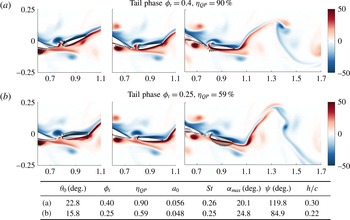
. The arrows plotted over the bodies represent the local pressure force observed at the surface of the fish. Reducing the tail phase reduces the inclination of the caudal fin as the negative induced vortex approaches on the left, reducing thrust generation. Furthermore, downstream, it can be seen that for
 $\unicode[STIX]{x1D719}_{t}=0.4$
, the positive vortex from upstream pairs up with a negative vortex shed from the trailing edge such that they cancel each other, while reducing the width of the wake. The variables used in the table are defined in table 1.

3.4.3 Importance of independent tail phasing
The phasing of the tail greatly affects the swimming efficiency. At the optimal body phase and a tail phase of
 $\unicode[STIX]{x1D719}_{t}=0.25$
, the efficiency is mediocre, at
 $\unicode[STIX]{x1D702}_{QP}=59\,\%$
. By fine tuning the phase of the tail to
 $\unicode[STIX]{x1D719}_{t}=0.4$
, the efficiency is increased by over 30 %. Although this change in phase results in modest changes to the wake (figure 8), the change to swimming efficiency is significant. The rise in efficiency is a result of two hydrodynamic mechanisms. First, at a tail phase of
 $\unicode[STIX]{x1D719}_{t}=0.4$
, the leftmost figure in 8(a) shows that the tail is more angled to the horizontal as the induced vortex approaches. This allows the tail to harness the low pressure core of the vortex to enhance thrust, as shown by the instantaneous local force arrows in figure 8(a). Second, at
 $\unicode[STIX]{x1D719}_{t}=0.4$
the vortex at the trailing edge sheds slightly later, and pairs up optimally with an oppositely signed vortex from the upstream wake (rightmost image in figure 8
a). This vortex pairing effectively cancels the induced velocity field created by the negative vortex at
 $x/L\sim 1.4$
. As already shown previously in figure 7(c), the cancellation of well-paired vortices reduces the detrimental lateral force observed by the caudal fin. Over time, vorticity annihilation occurs, yielding a weaker and slightly narrower overall wake.
These results demonstrate that the timing of a distinct tail is critical in the presence of vortices, and that independent pitch control of a distinct tail can be used to fine tune the interaction for significant hydrodynamic benefit. Although modifications to the tail phase affect the timing of only a small section of the fish, at the optimal body phase a change in tail phase of 0.15 can yield over a 30 % change to the efficiency.
3.5 Summary: sensitivity of efficiency for independently pitching tail
From a global perspective, the optimal tail phase depends on the swimming parameters of the upstream fish, the distance between them, the body undulation phase of the downstream fish and the additional swimming parameters of the downstream fish. However, on a local level the optimal tail pitch phase depends directly on the state of the induced vortex as it approaches the tail. Within this section, we described the physical interactions taking place to allow the fish to harness the energy of the induced vortex in an advantageous manner. Although the timing and spacing relative to the upstream fish may vary according to the exact swimming configurations of both, the hydrodynamic events happening on a local level can be consistently exploited by executing timing relative to the local vortices. By learning the ideal vortex-relative phase over time and using flow feedback to maintain the optimal vortex-relative timing, the fish can consistently harness energy through the mechanisms described here.
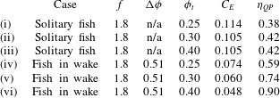
Table 2 summarizes the power expended
 $C_{E}$
and swimming efficiency
 $\unicode[STIX]{x1D702}_{QP}$
for various swimming configurations for a fish with an independently pitching tail. A fish swimming alone has efficiency around
 $\unicode[STIX]{x1D702}_{QP}=40\,\%$
. While changes to the tail pitch phase can change the efficiency by a few per cent, the effect is relatively small. For a fish within the wake of another fish, optimization of the body motion results in an efficiency of roughly
 $\unicode[STIX]{x1D702}_{QP}=59\,\%$
. Finally, by also optimizing the tail pitch phase, an efficiency of
 $90\,\%$
can be reached.
This shows that timing of the peduncle region of a fish with a distinct tail is crucial. Even more interestingly, it shows that at the optimal body phase, fine tuning of the tail pitch motion relative to the surrounding vortices can greatly improve the swimming performance. As the positions of surrounding vortices are very detectable and directly related to energy recovery mechanisms, coordination strategies can be devised to interact with the flow in hydrodynamically optimal ways.
Summary of the swimming efficiency for several swimming configurations. The variables used in the table are defined in table 1.
4 Sensing of near-field vortices
Fish through their lateral line have the ability to sense and respond to disturbances in their surrounding flow and make the kinematic adjustments necessary to control their body. Previous work has shown that this distributed sensing ability enables fish to identify objects, localize prey and execute formation control within schools (Pitcher et al. Reference Pitcher, Partridge and Wardle1976; Partridge & Pitcher Reference Partridge and Pitcher1980; Hassan Reference Hassan1989; Humphreys & Feinberg Reference Humphreys and Feinberg1995; Sharma et al. Reference Sharma, Coombs, Patton and de Perera2009). In addition, this sensory system enables fish to control their interaction with the surrounding flow in order to extract energy from waves, wakes and even turbulence (Triantafyllou & Triantafyllou Reference Triantafyllou and Triantafyllou1995; Liao Reference Liao2007).
Section 5 demonstrated that precise timing is critical for optimal energy extraction from a wake. Furthermore, this precise timing cannot be executed by vision alone, since the relevant mechanisms depend on the positions of surrounding vortices, which are not visible. Precise interaction with these vortices can give rise to remarkable swimming efficiencies, but the fish must be capable of accurately localizing near-field vortices. The swimming efficiency is reduced by over 15 % when the phase is
 $36^{\circ }$
away from the optimal value; therefore, the fish under study must localize vortices within an error of less than 5 % of its body length.
In this section, we describe a modelling and estimation approach capable of extracting the near-field vortex locations from distributed lateral line signals, within this error tolerance, demonstrating that the precise feedback required is feasible.
4.1 Lateral line measurements
While the lateral line system in fish is capable of detecting both water velocity through the superficial lateral line subsystem (SLLS) and pressure gradients through the canal lateral line subsystem (CLLS), we focus on the distributed pressure sensing ability in this project. Vortices in the near field may stimulate both the SLLS and the CLLS; however, within running water or when swimming at high speeds, the neuromasts within the SLLS may become saturated and insensitive to additional fluctuations in the water motion (Engelmann, Hanke & Bleckmann Reference Engelmann, Hanke and Bleckmann2002). In contrast, the CLLS neuromasts, which reside within subdermal canals, are not saturated during steady swimming.
Prior research has demonstrated that the distributed pressure signal captured by the CLLS can be used to characterize vortices in the near field (Suzuki & Colonius Reference Suzuki and Colonius2003; Fernandez Reference Fernandez2011; Ren & Mohseni Reference Ren and Mohseni2012). These studies show that in the absence of strong interaction with the sensing body, near-field vortices can be localized well. In this paper, we demonstrate that even with the strong interactions that give rise to the formation of body-generated vortices, a fish swimming within the wake of another fish can still use the CLLS signal to accurately localize surrounding vortices.
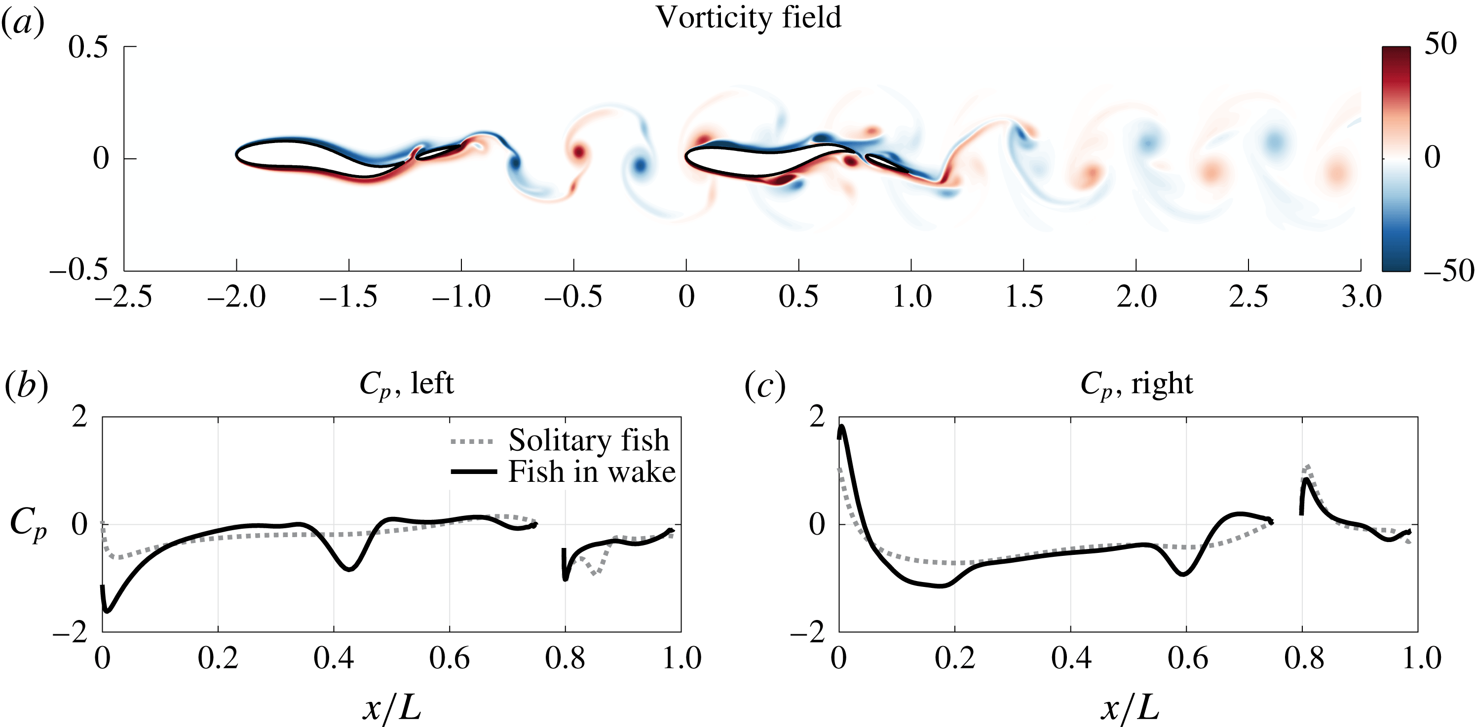
Within the simulation, an idealized lateral line sensor array is assumed to measure the pressure on the surface of the fish. A snapshot of the pressure sensed is shown in figure 9. For discrete lateral line measurements, values are interpolated from this idealized signal.
(a) A snapshot of the vorticity field generated when a fish swims at a distance of one body length directly downstream from another fish. The lower plots show, for the same time step, a snapshot of the pressure induced on the (b) left and (c) right sides of the downstream fish, compared with the pressure that would be experienced by a solitary fish swimming with the same kinematics.

Within the wake of the upstream fish, the downstream fish encounters a row of vortices of alternating sign. As each vortex approaches the nose of the fish, the stagnation point is shifted such that the pressure rises on one side while dropping on the other, creating a highly detectable signal. As the downstream fish encounters the oncoming wake, interaction with each oncoming vortex induces the formation of a secondary vortex. The formation of the induced vortex is associated with a significant low pressure dip at the nose of the fish. The signal along the body of the fish is dominated by the induced vortices (figure 9). The original vortices from the upstream wake are masked by the induced vortices along the body, and become largely unobservable after they pass the nose.
To execute appropriate timing, it is critical for the fish to detect the phase of the oncoming vortex street, as well as the position of induced vortices along the body. Control of the body undulation phase is performed relative to the phase of the upstream vortices, while control of the tail pitch is performed relative to the induced vortices along the body.
4.2 Potential flow model and validation
A two-dimensional potential flow model was developed to provide a low-order representation of the fish–vortex system, which is a requirement for a well-conditioned estimation (inverse) problem. The model functions to relate a reduced number of states which characterize the near-field flow to the hydrodynamic pressure distribution captured by the lateral line. Within the forward model formulation, the states of nearby vortices are used as an input; however, within the inverse problem, these vortex states are the unknowns to be estimated.
While potential flow methods have been used in the past with success as forward models of swimming fish (Barrett et al. Reference Barrett, Triantafyllou, Yue, Grosenbaugh and Wolfgang1999; Zhu et al. Reference Zhu, Wolfgang, Yue and Triantafyllou2002), it should be noted that such elaborate models are not required and in fact may be detrimental for an inverse model, because of the intense computational effort they require. In forward modelling, fluid states are predicted in succession, so that errors over many time steps build up to result in an ultimately inaccurate fluid state. In contrast, for inverse models, small errors are acceptable, as the model must only predict the measurements yielded by a single fluid state at a time. As a new measurement is collected at each time step, there is no need to predict the successive evolution of fluid states. As a result, even simple potential flow models have been used with great success in inverse modelling (Maertens Reference Maertens2011). In fact, the complication of additional complexity often results in poor conditioning of the inverse problem and increased estimation error. Therefore, it is more important to develop a low-order model which captures the local unsteady wake effects, rather than a higher-order model that captures the full flow physics and entire wake history which unnecessarily complicates controller and observer design (Izraelevitz, Zhu & Triantafyllou Reference Izraelevitz, Zhu and Triantafyllou2017).
Following the methodology outlined by Katz & Plotkin (Reference Katz and Plotkin2001), the body of the fish is modelled with a panel method consisting of
 $N=200$
discrete constant-strength source panels. Near-body vortices are represented as point vortices; a single point vortex is used for the vortices emanating from the upstream fish, while three closely spaced vortices are used to model each induced vortex. As such, each vortex is represented using only three states. Through solving a boundary value problem which ensures the satisfaction of the no-flux condition on the surface of the fish, the strength of each panel can be determined, and Bernoulli’s unsteady pressure law is used to solve for the pressure on each panel.
The Kutta condition, which governs vorticity shed at the trailing edge of the fish, was omitted in this case, as models including the Kutta condition did not perform significantly better than models without it. Both models fail to capture the pressure accurately near the trailing edge of the fish, where viscous effects are greater and the assumption of ideal flow fails. However, as the vortices are highly detectable at the nose and along the body of the fish, their positions near the tail can be tracked relatively accurately despite the less ideal performance of the model in this region. Along the majority of the fish body, a model excluding the Kutta condition performs just as well as that with it, and averts the complexity associated with the iterative schemes required to solve a pressure Kutta condition.
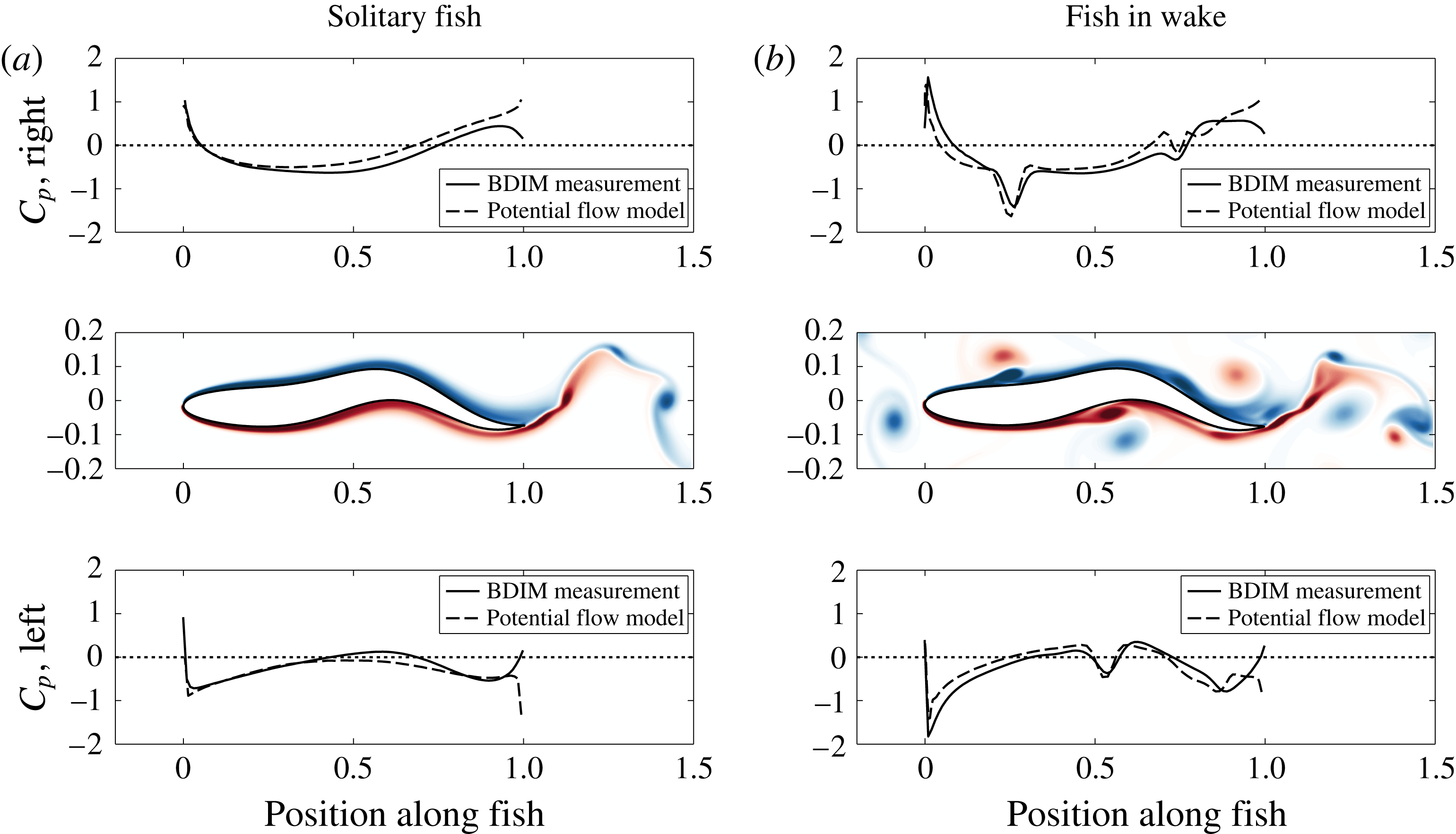
This potential flow model was validated for a continuous fish swimming alone, and also for the same fish within a wake. For the fish within a wake, the position and strength of near-field vortices were estimated from the vorticity field data collected within the BDIM simulation. A comparison between the pressure measured with the BDIM simulation and the pressure predicted by the potential flow model is shown in figure 10, for these two cases.
Validation of the potential flow forward model for (a) a fish swimming in quiescent water and (b) a fish swimming within a wake. Each plot shows a comparison between the pressure estimated with the source panel method model (dashed line) and the pressure measured within the BDIM simulation (solid line), for the left and right sides of the fish at an instant in time. The middle plots shows a snapshot of the vorticity field from the BDIM simulation. The colour bar for the vorticity field is the same as in figure 2.

Figure 10(a) shows a comparison between the modelled (potential flow) and actual (BDIM) pressure signals for a fish in quiescent water. It can be seen that the accuracy is high in the front half of the fish, and the error grows toward the back. This is expected – near the front of the fish the pressure gradient is favourable and viscous effects are negligible. However, near the back, the boundary layer thickens and viscous effects become more prominent.
Figure 10(b) shows a comparison between the modelled (potential flow) and actual (BDIM) pressure signals for a fish within a wake. The potential flow model is capable of capturing with reasonable accuracy both the large-scale pressure changes that result from its own undulating motion and the upstream vortices, and the small-scale pressure dips produced by the induced vortices along the body. While there is some error between the modelled and actual pressure, the error is remarkably low given the significant interaction between the fish and the wake. In particular, the error near the nose is small, and the low pressure minima created by vortices along the body are captured very well. Conveniently, for energy extraction within a wake, the strongest interactions, which yield the highly observable signals created by the upstream vortices and the induced vortices along the body, are also the most important to capture.
We employ a panel method as a low-order approximation model to relate the states of near-field vortices with the pressure sensed on the surface of the fish. Through matrix formulation, this forward problem can be solved rapidly, and much faster than the BDIM simulation described in § 2. Due to its ability to (i) be solved quickly, (ii) model the surrounding flow using a low number of states and (iii) capture the interaction between the undulating fish and the surrounding flow accurately, we determined that this model would be suitable to use within the inverse problem of estimating near-field vortices using lateral line feedback.
4.3 Vortex state estimation
An unscented Kalman filter (UKF) was implemented to solve the inverse problem of estimating the states of near-field vortices using the distributed pressure measurements captured by the lateral line, following the methodology outlined by Julier & Uhlmann (Reference Julier and Uhlmann2004).
The estimation of surrounding vortices is divided into three distinct parts: (i) estimation of the approaching vortex street, (ii) identification and tracking of the induced vortex and (iii) dead reckoning for characterization of the original vortex at the tail. Each estimation task uses only a subset of the sensors available on the body.
For the first task, estimation of the approaching vortex street, the UKF at the head estimates four states to characterize the oncoming vortex street:
 $\boldsymbol{x}_{1}=[x;y;\unicode[STIX]{x1D6FE};\unicode[STIX]{x1D706}]$
.
 $(x,y)$
is the position of the closest approaching vortex upstream of the nose,
 $\unicode[STIX]{x1D6E4}$
is the circulation of the vortex and
 $\unicode[STIX]{x1D706}$
is the wavelength of the upstream vortex street. This state characterizes a set of three vortices from the wake of the upstream fish, around the nose of the downstream fish.
A second UKF estimates the strength of the induced vortex along the body, while the position of the vortex is inferred from the pressure minimum along the body. Finally, the forward model only is used to estimated the position of the original vortex as it reaches the tail, with no feedback from pressure measurements.
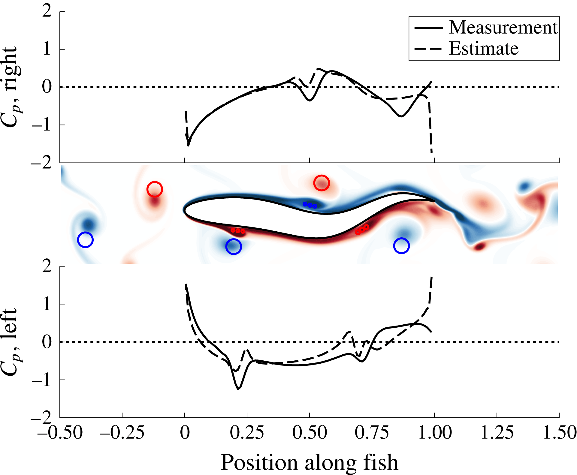
The performance of the estimation scheme at one instance is shown in figure 11, for a fish with a continuous body (no separate caudal fin). As shown, the position and strength of each vortex in the near field is captured extremely accurately. While there is some error in the lateral position estimate of the upstream wake vortices, this is expected, and not important. Since the upstream vortices are estimated as a set of three vortices, characterized by only four states, it is impossible to capture the lateral position of each perfectly. However, with some tuning, very high accuracy of the streamwise position estimate for the oncoming vortices can be attained. The streamwise positions of the induced vortices are very observable, and are estimated very accurately along the body.
Validation of the vortex estimation scheme. The middle plot shows a snapshot of the vorticity field, with the circles showing the estimated positions of all near-field vortices (red for positive and blue for negative). The colour bar for the vorticity field is the same as in figure 2. The other two plots show a comparison between the actual pressure (measured in the BDIM simulation) and the estimated pressure (estimated using the estimated vortex positions and the potential flow model). The upstream wake vortices and the vortices along the body are estimated using three different strategies, as described in the text. Induced vortices are modelled using three closely spaced point vortices, as shown.

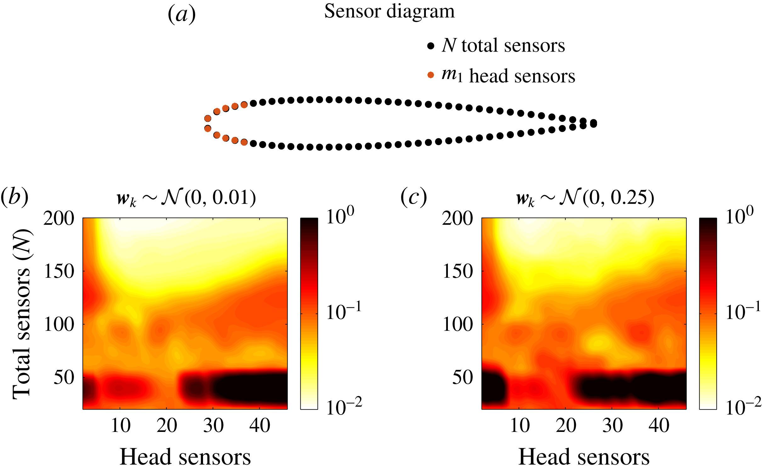
In an actual implementation, measurements are corrupted by noise. Figure 12 illustrates the average error in the estimated streamwise position of the upstream wake vortices, given two different levels of Gaussian white noise.
The average error in the streamwise position estimate, for upstream wake vortices at
 $x/L=0$
, with (a) a small amount of Gaussian white measurement noise, and (b) with measurement noise of variance that exceeds the variance of the pressure signal itself.

With a low level of noise (
 $\unicode[STIX]{x1D70E}^{2}=0.01$
), figure 12(b) shows that the UKF can extract the streamwise position of the upstream wake vortices within an error of 0.7 % of the body length, using
 $m_{1}=16$
sensors at the nose, at a density of
 $N=200$
sensors over the entire body. Furthermore, for
 $N>150$
, the estimation error is generally low (within 2 % of the body length, for
 $10<m_{1}<34$
). Since the formation of induced vortices is not included in the potential flow model, estimation is most accurate when pressure measurements within the front 20 % of the body are used for feedback.
With a high level of measurement noise (
 $\unicode[STIX]{x1D70E}^{2}=0.25$
), figure 12(c) shows that the UKF can still extract the streamwise position of the upstream wake vortices within an error of 2 % of the body length, using
 $10<m_{1}<25$
sensors at the nose at a density of
 $N>150$
sensors over the body. For reference, the mean variance of pressure measurements over the nose of the fish is
 $\unicode[STIX]{x1D70E}^{2}=0.22$
, so in the high noise case, the measurement noise varies as much as the pressure signal at the nose.
In summary, even with significant measurement noise, it is feasible for the distributed pressure sensing capability of the lateral line to provide the precise feedback required for the fish to execute precise vortex-relative control.
5 Active flow control
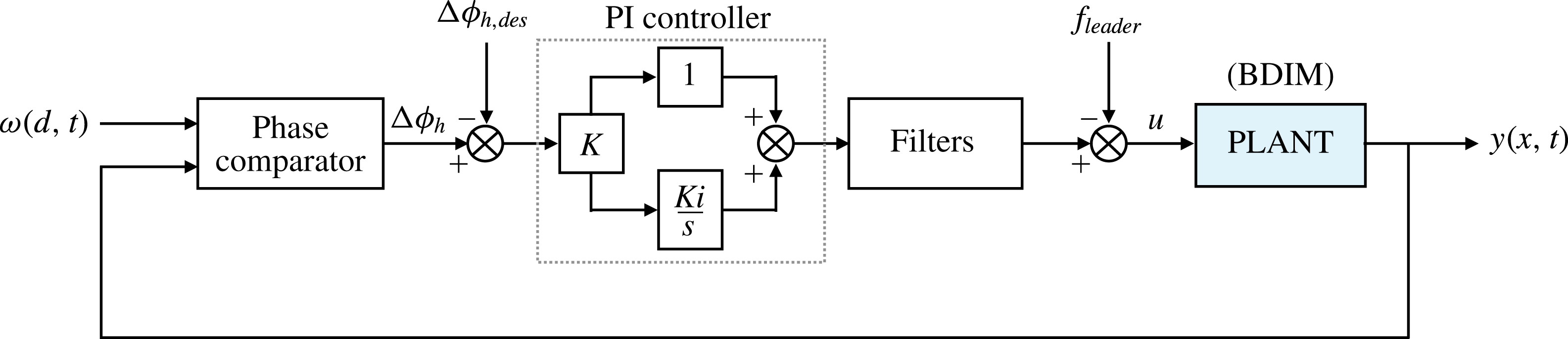
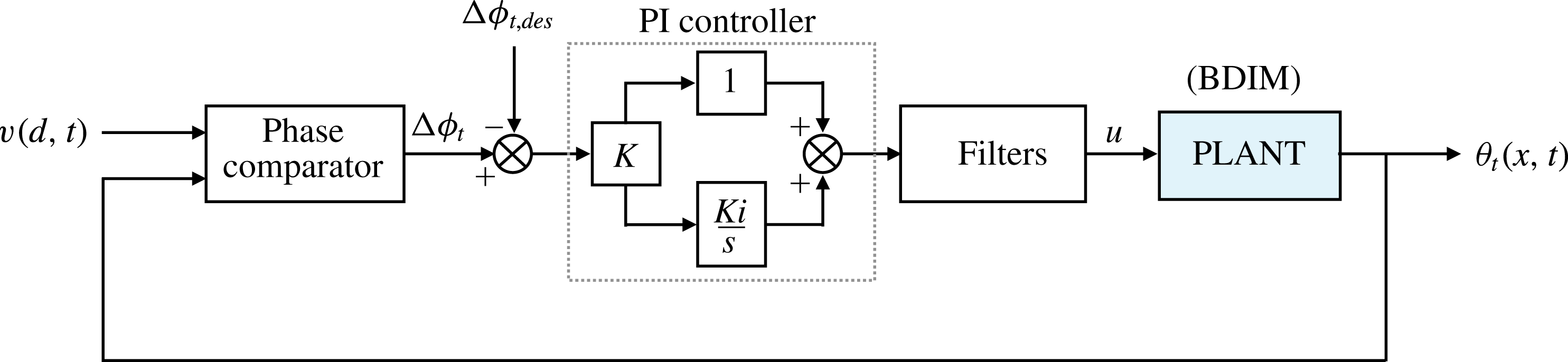
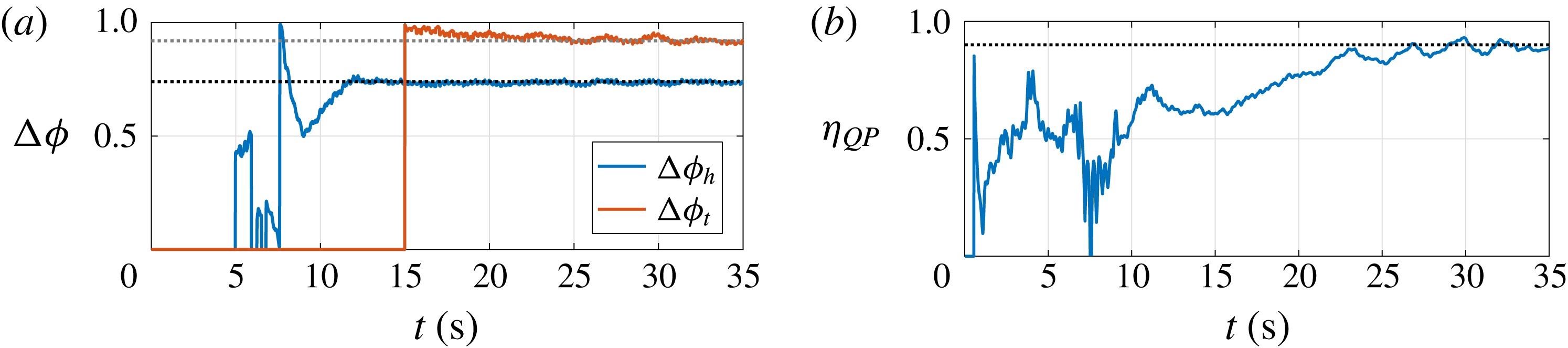
Using the precise feedback described in § 4.3, the downstream fish can time its motion relative to vortices in the surrounding flow. Section 3 demonstrated that with a distinct tail, the phasing of the body undulating motion and the independent timing of tail pitch motion are both extremely important. To optimally harness energy from the upstream wake, the fish must control its motion to synchronize to the upstream wake frequency and establish the most advantageous phase relationship. While the optimal phase has been defined in relation to the upstream fish, § 3 demonstrated that the interactions occurring on a local level drive the ideal timing. The mechanisms behind and timing of these local interactions remain consistent despite changes to the swimming configuration. Additionally, fine tuning of the tail pitch motion relative to approaching induced vortices can yield a significant further increase to the swimming efficiency. In this section, we will show that a phase-locked loop controller can use the estimated vortex positions provided by the estimator in order to drive a fish toward the optimal phase relationships.
In order to keep the control problem computationally tractable, the following assumptions were made:
(i) The optimal vortex-relative phase is learned a priori. For the current system, this learning process has effectively been performed by the optimization routine.
(ii) The first PID controller, which adjusts
 $a_{0}$
to regulate swimming speed (§ 2.4), acts fast enough to keep the fish at a constant distance behind an upstream fish. This allows us to simulate the control system on a fish with fixed streamwise position, greatly reducing the time required for convergence.
(iii) The upstream wake is general regular, so that the control system can be designed to operate on the timescale of several tail-beat periods, rather than within a single period.
(iv) We assume that the downstream fish can see the upstream fish, allowing it to stay centred within the wake of the upstream fish. Alternatively, algorithms such as developed in Beal et al. (Reference Beal, Hover, Triantafyllou, Liao and Lauder2006) can be used to centre the fish within an oncoming wake.

5.1 Phase-locked loop controller
Fish are known to synchronize their tail-beat frequency to the frequency of an external source, even when that frequency is significantly different from their own (Liao et al. Reference Liao, Beal, Lauder and Triantafyllou2003a ,Reference Liao, Beal, Lauder and Triantafyllou b ). In order to capture energy from the upstream wake, the downstream fish must first synchronize to the frequency of the upstream wake. To perform this synchronization, a phase-locked loop controller was implemented.
Diagram of the phase-locked loop controller for the body undulation.

Diagram of the phase-locked loop controller for the tail pitch phase.

The phase-locked loop (PLL) controller compares the phase of an input signal with that of an output signal, and adjusts the frequency or phase of the system in response. Figure 13 shows a diagram of the PLL controller which drives the body undulatory phase toward the optimal phase relative to the upstream wake vortices, and figure 14 shows a diagram of the PLL controller that drives the tail pitch phase toward the optimal relative to the induced vortices within the system. Each controller consists of three basic parts: (i) the phase comparator, which compares the phase of vortices with the motion of the fish, (ii) a proportional-integral (PI) controller that drives the phase difference toward a desirable value and (iii) a few filters to smooth out noise.
5.2 Active wake-relative control
Simulation with active sensing and body control were conducted with the upstream fish swimming at a constant velocity of
 $U_{l}=1$
and frequency
 $f_{l}=1.8$
, and the following fish at
 $U_{f}=1$
and
 $f_{f}=1.7$
. In order to consistently extract energy from the upstream wake, the following fish must synchronize to the upstream wake frequency and converge to the optimal phase difference of
 $\unicode[STIX]{x0394}\unicode[STIX]{x1D719}_{h}=0.74,~\unicode[STIX]{x0394}\unicode[STIX]{x1D719}_{t}=0.92$
, using feedback from the lateral line.
The desired phase difference for the tail controller is only valid at
 $\unicode[STIX]{x0394}\unicode[STIX]{x1D719}_{h}=0.74$
, since the development of induced vortices along the body depends directly on the interaction with the upstream wake. Therefore, the body controller works first to drive the body undulation phase toward the optimal value, and subsequently the tail controller drives the tail pitch phase difference to the desired value.
(a) The estimated head and tail phase differences and (b) the period-averaged efficiency over time, for a fish which first converges to the desired body undulation vortex-relative phase
 $\unicode[STIX]{x0394}\unicode[STIX]{x1D719}_{h}$
, and activates the tail control at
 $t=15$
.

Figure 15 shows simulation results when the two PLL controllers successfully drive the fish to the optimal swimming configuration within the wake of an upstream fish. Figure 15(a) shows that both controllers converge to the desired vortex-relative phase differences quickly. In the beginning of the simulation, approximately 5 s are required for the vortices from the leading fish to reach the following fish, and for the flow state to reach a fully developed state. Following this (
 $t=5$
), the vortex estimator requires a short amount of time to converge to an accurate estimate of the upstream wake. After the estimator converges (
 $t=6.5$
), the body phase controller converges to the desired phase within about 5 s, or 10 swimming periods. After the tail controller is activated at
 $t=15$
, the tail pitch phase converges to the desired value in approximately 10 s. Figure 15(b) shows that shortly after this, the period-averaged efficiency converges to the optimal value of
 $\unicode[STIX]{x1D702}_{QP}=90\,\%$
.
Figure 16 shows vorticity snapshots of the flow surrounding the fish before the body phase controller has converged (a–c), after the body phase controller has converged (d,e) and after the tail controller has converged (f), in order to better illustrate the flow patterns over time and the corresponding swimming performance. While the body controller is working to drive the body phase toward the ideal phase difference, the amplitude of undulation and efficiency vary wildly, along with the downstream wake. Changes to the phase dramatically affect the interaction between the entire body of the fish and the upstream wake. The interactions vary between being beneficial and detrimental, and the overall efficiency hovers around 50 %–60 %.
Vorticity snapshots of the fish (a–c) before the body phase controller has converged, (d,e) after the body phase controller has converged and after the tail controller is activated and (f) after the tail controller has converged. The colour bar for the vorticity field is the same as in figure 2.

Even after the body phase has converged (figure 16
d), the efficiency is still quite low. However, this step is necessary, as the range of feasible tail phases is fundamentally limited and the induced vortices must be properly positioned to allow for the tail to exploit them within its own constraints. However, once the body is properly phased, as shown in figure 15(a), the greatest change to the efficiency occurs between
 $t=15$
and
 $t=25$
, as the tail motion is fine tuned. As seen in the last three snapshots of figure 16, although the flow field looks quite similar in
 $t=15.24$
and subsequent time steps, this fine tuning of the tail motion results in a 30 % increase to the efficiency. This is similar to the results shown in § 3.4.3; the dramatic rise in efficiency results from precise vorticity control. While the previous result was obtained in open loop (without feedback), the present demonstration shows that the fish can execute this precise control using only the distributed sensing ability provided by the lateral line. Although it is unlikely for a fish to accurately time its motion relative to an upstream fish by visual feedback alone, the local pressure feedback acquired along its body allows it to establish the precise vortex-relative phase that gives rise to the optimal efficiency.
In summary, using the sensor information developed in § 4, we show that fish can actively synchronize to the frequency of an upstream wake at the correct phase, and fine tune their tail motion to optimally exploit the wake. As described in § 3.5, while some energy can be harnessed from the wake without precise timing, the energy savings is greatly increased when the optimal phasing is executed. Together, distributed flow sensing and vorticity control provide a powerful tool to control the flow for enhanced swimming performance.
6 Conclusions
We study through two-dimensional simulation the optimal energy extraction mechanisms of a self-propelled fish swimming within the wake of an identical self-propelled upstream fish. There are three central conclusions of the study:
(i) A fish in the wake of an upstream fish needs less than half the power to self-propel than in open water, achieving quasi-propulsive efficiency of 90 % when using optimal body and tail motion for energy extraction from the vortices generated by the upstream fish. The head of the fish must move in a slaloming motion among the oncoming vortices, and, more critically, the independently controlled pitching motion of the tail must employ vorticity annihilation for this efficiency to materialize (figures 4–7).
(ii) The location of the oncoming vortices and the induced vortices can be localized with high accuracy using distributed pressure measurements along the body of the fish, such as those obtained from the lateral line of a fish, to drive an unscented Kalman filter.
(iii) Closed loop control can use the estimated location of the near body vortices by the Kalman filter to optimize the body and tail motion of the fish to stably converge to the optimal gait, obtaining the same high efficiency identified through parametric optimization.
High efficiency is found over a narrow parametric range and is possible only when the caudal fin is allowed to pitch independently from the motion of the main body. Consequently, closed loop control also requires an independently controlled caudal fin. This is the first study, to the authors’ knowledge, which shows that such dramatic increases in efficiency can be achieved through vorticity control with a distinct tail when schooling.
In conclusion, artificial lateral lines that are currently under development (Triantafyllou et al. Reference Triantafyllou, Weymouth and Miao2016), which can potentially be used with the algorithms developed in this paper to drive controllers to extract energy and achieve high propulsive efficiency in schooling fish-like robots.
Acknowledgements
The authors wish to acknowledge support from the Singapore-MIT Alliance for Research and Technology through the CENSAM Program, and from the MIT Sea Grant Program.
Appendix. Numerical method validation
BDIM has been validated for several single and multi-body body problems, including the flow past a circular cylinder, the flow past an asymmetric foil at an angle of attack, a foil gliding by a cylinder, the flow induced vibration of a circular cylinder and the impact of a blunt body on a free surface (Weymouth & Yue Reference Weymouth and Yue2011; Maertens Reference Maertens2015). In Maertens & Weymouth (Reference Maertens and Weymouth2015), the method was validated for both stationary and heaving and pitching airfoils at Reynolds numbers of
 $Re=10\,000$
and above, and found to produce good agreement with the literature. Cartesian grid methods are also well established for problems with multiply connected domains (Ye et al.
Reference Ye, Mittal, Udaykumar and Shyy1999; Weymouth et al.
Reference Weymouth, Dommermuth, Hendrickson and Yue2006).
Furthermore, BDIM has been used successfully to study problems involving shedding of vorticity from retracting foils (Wibawa et al. Reference Wibawa, Steele, Dahl, Rival, Weymouth and Triantafyllou2012), deformable jet-propelled bodies (Weymouth & Triantafyllou Reference Weymouth and Triantafyllou2013; Steele, Weymouth & Triantafyllou Reference Steele, Weymouth and Triantafyllou2017), flow control with rotating cylinders (Schulmeister et al. Reference Schulmeister, Dahl, Weymouth and Triantafyllou2017) and the unsteady aerodynamics of perching (Polet et al. Reference Polet, Christensen, Rival and Weymouth2014; Polet, Rival & Weymouth Reference Polet, Rival and Weymouth2015). These demonstrate the ability of BDIM to handle simulations with multiple and deforming bodies accurately, involving problems with small details or gaps.
For the present study, a grid refinement study was performed for a NACA0012 at
 $Re=5000$
, and
 $0^{\circ }$
and
 $5^{\circ }$
relative to the oncoming flow. Figure 17 shows the error in the friction and pressure drag as a function of grid resolution. At the finest resolution, the error is within 10 %, and remains bounded at higher resolutions.
Time-averaged friction and pressure drag (
 $C_{Df}$
and
 $C_{Dp}$
, respectively) on a NACA0012 at
 $Re=5000$
and angle of attack
 $\unicode[STIX]{x1D6FC}=0^{\circ }$
and
 $5^{\circ }$
, as a function of grid resolution. The absolute value of the relative error
 $E$
is computed with respect to XFOIL:
 $E=|C_{D_{\text{BDIM}}}/C_{D_{\text{XFOIL}}}-1|$
. Figure adapted from Maertens et al. (Reference Maertens, Gao and Triantafyllou2017).