1. Introduction
The flow in precessing rapidly rotating containers has a long history; the early works are comprehensively covered in Greenspan (Reference Greenspan1968). The problem is interesting not only from a fundamental perspective, but also due to its prominence in a wide range of applications. These include astrophysical and geophysical flows (Malkus Reference Malkus1968; Tilgner Reference Tilgner2005; Nore et al.
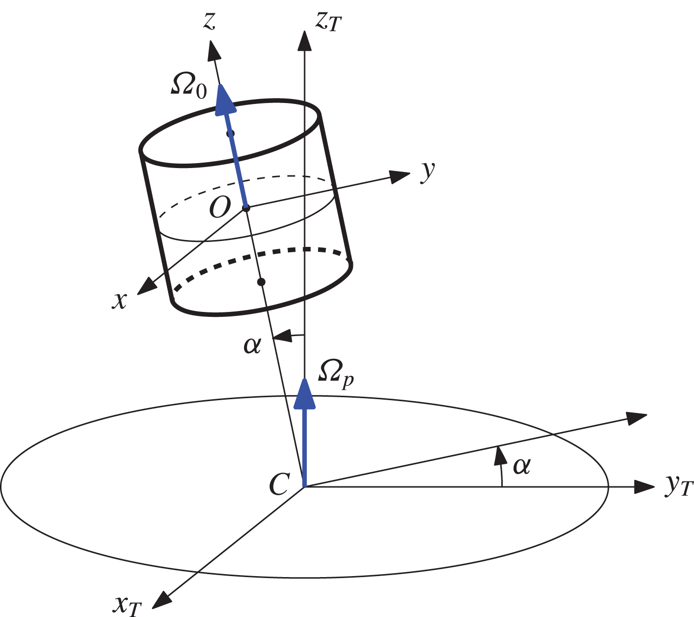
Reference Nore, Léorat, Guermond and Luddens2011), and engineering applications (Manasseh Reference Manasseh1993; Johnston Reference Johnston1998). A canonical example of a precessing flow consists of a rapidly rotating cylinder with angular velocity
 ${\it\Omega}_{0}$
, with the cylinder axis rotating with angular velocity
 ${\it\Omega}_{p}$
around another axis; see figure 1. The angle
 ${\it\alpha}$
between the two axes is called the nutation or tilt angle. When the tilt angle
 ${\it\alpha}$
is zero or the precessing frequency
 ${\it\Omega}_{p}$
is zero, the flow in the rotating cylinder is stable solid-body rotation. The limits
 ${\it\alpha}\rightarrow 0$
and
 ${\it\Omega}_{p}\rightarrow 0$
are singular in the sense that the symmetries of the problem in the limit are completely different from the symmetries of the problem at either
 ${\it\alpha}=0$
or
 ${\it\Omega}_{p}=0$
, and this impacts on the nature of the instabilities of the flow.
Schematic of the precessing cylinder and the different frames of reference involved. The axis
 $(x_{T},y_{T},z_{T})$
and
 $(x,y,z)$
are fixed on the rotating table, with origin at
 $C$
and
 $O$
, the cylinder and table centers, respectively;
 ${\it\alpha}$
is the constant tilt angle,
 ${\it\Omega}_{p}$
is the angular velocity of the table and
 ${\it\Omega}_{0}$
is the angular velocity of the cylinder with respect to the rotating table.

The early theory was also developed in the singular inviscid limit and in the limit of vanishingly small nonlinearities. Lord Kelvin (Reference Lord Kelvin1880) solved the inviscid Navier–Stokes equations (Euler equations) linearized about solid-body rotation; by assuming a perturbation with a single temporal frequency, an eigenvalue problem is obtained, and its solutions are the so-called Kelvin modes which only exist for perturbation frequencies less than two times the solid-body rotation frequency. These neutral modes are damped by viscosity, and any physical realization of these modes with finite viscosity requires an external forcing to excite them. The cylinder precession in our problem corresponds to a body force that drives a Kelvin mode with azimuthal wavenumber
 $m=1$
due to the tilt of the rotation axis. In a physical cylinder, the no-slip boundary conditions lead to the formation of viscous boundary layers, and together with nonlinearity of the system, an axisymmetric azimuthal mean flow results, essentially via steady streaming (Riley Reference Riley2001). It is expected to be essentially independent of the axial direction except in the boundary layer, and so is often referred to as the geostrophic mode (Greenspan Reference Greenspan1968).
The aspect ratio of the cylinder and the precession frequency
 ${\it\Omega}_{p}$
can be tuned so that various Kelvin modes can ‘fit’ into the cylinder. McEwan (Reference McEwan1970), based on experiments in a related flow, suggested that for an appropriately tuned precessing cylinder, two other Kelvin modes can form a resonant triad with the forced
 $m=1$
mode and lead to complex flows, along the lines outlined in Kerswell (Reference Kerswell1999, Reference Kerswell2002). Manasseh (Reference Manasseh1992, Reference Manasseh1994) observed such flows in precessing cylinder experiments, and Lagrange et al. (Reference Lagrange, Eloy, Nadal and Meunier2008, Reference Lagrange, Meunier, Nadal and Eloy2011) developed a linear and weakly nonlinear theory that accounted for some of the viscous effects to predict the triadic resonances and compared the theoretical results with laboratory experiments. The agreement was generally very good, although details of the bifurcations involved were unresolved due to experimental limitations. They focused on the first resonance of the forced Kelvin mode where free Kelvin modes with azimuthal wavenumbers
 $m=5$
and
 $m=6$
are excited. It is this same resonance that we focus our nonlinear numerical study on here.
2. Governing equations and numerical scheme
Consider a cylinder of height
 $H$
and radius
 $R$
filled with an incompressible fluid of kinematic viscosity
 ${\it\nu}$
. All variables are non-dimensionalized using the cylinder radius
 $R$
as the length scale and the viscous time
 $R^{2}/{\it\nu}$
as the time scale. The cylinder is mounted at the centre
 $C$
of a horizontal table that rotates with angular velocity
 ${\it\Omega}_{p}$
around the vertical axis
 $z_{T}$
, as shown in figure 1. The cylinder axis is tilted an angle
 ${\it\alpha}$
relative to the vertical, and is at rest relative to the table, therefore the cylinder axis precesses with angular velocity
 ${\it\Omega}_{p}$
with respect to the laboratory inertial reference frame. Moreover, in the table reference frame, the cylinder rotates around this tilted axis with angular velocity
 ${\it\Omega}_{0}$
.
There are four independent non-dimensional parameters governing the flow:
 $$\begin{eqnarray}\displaystyle & \displaystyle \text{cylinder rotation}\quad {\it\omega}_{0}={\it\Omega}_{0}R^{2}/{\it\nu}, & \displaystyle\end{eqnarray}$$
 $$\begin{eqnarray}\displaystyle & \displaystyle \text{precession rate}\quad {\it\omega}_{p}={\it\Omega}_{p}R^{2}/{\it\nu}, & \displaystyle\end{eqnarray}$$
 $$\begin{eqnarray}\displaystyle & \displaystyle \text{aspect ratio}\quad {\it\Gamma}=H/R, & \displaystyle\end{eqnarray}$$
 $$\begin{eqnarray}\displaystyle & \displaystyle \text{tilt angle}\quad {\it\alpha}. & \displaystyle\end{eqnarray}$$
 $\mathit{Re}={\it\omega}_{0}+{\it\omega}_{p}\cos {\it\alpha}$
, the Rossby number
 $\mathit{Ro}={\it\omega}_{p}\sin {\it\alpha}/\mathit{Re}$
, the forcing frequency
 ${\it\omega}_{f}={\it\omega}_{0}/Re$
and the Poincaré number
 ${\it\omega}_{p}/{\it\omega}_{0}=(1/{\it\omega}_{f}-1)/\text{cos}{\it\alpha}$
.
The product
 $\mathit{Re}\mathit{Ro}$
is used (Lagrange et al.
Reference Lagrange, Eloy, Nadal and Meunier2008, Reference Lagrange, Meunier, Nadal and Eloy2011) as a measure of the strength of the precessional forcing. In terms of our parameters,
 $\mathit{Re}\mathit{Ro}={\it\omega}_{p}\sin {\it\alpha}$
, and it clearly shows that the strength of the precessional forcing has two contributing factors, how fast the table is rotating (relative to the viscous time) and how large the tilt angle is. In the absence of viscous effects, the individual values of the two factors are not important, only their product is, and so in many theoretical treatments (e.g. Mahalov Reference Mahalov1993; Lehner et al.
Reference Lehner, Mouhali, Leorat and Mahalov2010) a tilt angle of
 ${\it\alpha}=90^{\circ }$
is used. However, viscous effects do make material differences for different values of
 ${\it\alpha}$
when
 ${\it\omega}_{p}\sin {\it\alpha}$
is fixed, due to boundary layer deformations and even separations when both
 ${\it\alpha}$
and
 ${\it\omega}_{p}\sin {\it\alpha}$
are large (e.g. Kong, Liao & Zhang Reference Kong, Liao and Zhang2014; Kong et al.
Reference Kong, Cui, Liao and Zhang2015). As noted by Greenspan (Reference Greenspan1968), the sidewall boundary layer in the precessing cylinder is not simply due to an Ekman-like balance between Coriolis force and pressure gradient, but is rather more subtle.
The governing equations are written using cylindrical coordinates
 $(r,{\it\theta},z)$
, fixed in the rotating table frame of reference, with the
 $z$
direction aligned with the cylinder axis and the origin
 $O$
at the centre of the cylinder, as shown in figure 1. The fluid domain is given by
 $\mathscr{D}=\{(r,{\it\theta},z)\in [0,1]\times [0,2{\rm\pi}]\times [-{\it\Gamma}/2,{\it\Gamma}/2]\}$
. As this reference frame is non-inertial, the Navier–Stokes equations include four inertial terms as body forces:
 $$\begin{eqnarray}\partial _{t}\boldsymbol{v}+(\boldsymbol{v}\boldsymbol{\cdot }\boldsymbol{{\rm\nabla}})\boldsymbol{v}=-\boldsymbol{{\rm\nabla}}p_{0}-\frac{\text{d}^{2}\overrightarrow{CO}}{\text{d}t^{2}}-\frac{\text{d}{\bf\omega}_{p}}{\text{d}t}\times \boldsymbol{r}-2{\bf\omega}_{p}\times \boldsymbol{v}-{\bf\omega}_{p}\times ({\bf\omega}_{p}\times \boldsymbol{r})+{\rm\Delta}\boldsymbol{v},\end{eqnarray}$$
where
 ${\bf\omega}_{p}$
is the angular velocity vector of the reference frame considered
 $\{O;x,y,z\}$
with respect to the laboratory inertial reference frame. In Cartesian
 $\{\hat{\boldsymbol{x}},\hat{\boldsymbol{y}},\hat{\boldsymbol{z}}\}$
and cylindrical
 $\{\hat{\boldsymbol{r}},\hat{{\bf\theta}},\hat{\boldsymbol{z}}\}$
coordinates, its components are
 $$\begin{eqnarray}{\bf\omega}_{p}={\it\omega}_{p}\sin {\it\alpha}\,\hat{\boldsymbol{y}}+{\it\omega}_{p}\cos {\it\alpha}\,\hat{\boldsymbol{z}}={\it\omega}_{p}\sin {\it\alpha}\sin {\it\theta}\,\hat{\boldsymbol{r}}+{\it\omega}_{p}\sin {\it\alpha}\cos {\it\theta}\,\hat{{\bf\theta}}+{\it\omega}_{p}\cos {\it\alpha}\,\hat{\boldsymbol{z}}.\end{eqnarray}$$
This vector depends explicitly on the azimuthal coordinate
 ${\it\theta}$
due to the tilt angle
 ${\it\alpha}$
, but is independent of time, and so the second inertial term in (2.5) is zero. Moreover, the first and last inertial terms (acceleration of
 $O$
and the centrifugal term) are gradients and can be included in the pressure gradient term:
 $$\begin{eqnarray}\frac{\text{d}^{2}\overrightarrow{CO}}{\text{d}t^{2}}+{\bf\omega}_{p}\times ({\bf\omega}_{p}\times \boldsymbol{r})=\boldsymbol{{\rm\nabla}}\left(\frac{\text{d}^{2}\overrightarrow{CO}}{\text{d}t^{2}}\boldsymbol{\cdot }\boldsymbol{r}-\frac{1}{2}|{\bf\omega}_{p}\times \boldsymbol{r}|^{2}\right).\end{eqnarray}$$
The governing equations are
 $$\begin{eqnarray}\partial _{t}\boldsymbol{v}+(\boldsymbol{v}\boldsymbol{\cdot }\boldsymbol{{\rm\nabla}})\boldsymbol{v}=-\boldsymbol{{\rm\nabla}}p-2{\bf\omega}_{p}\times \boldsymbol{v}+{\rm\Delta}\boldsymbol{v},\quad \boldsymbol{{\rm\nabla}}\boldsymbol{\cdot }\boldsymbol{v}=0,\end{eqnarray}$$
where now
 $p$
includes contributions from the acceleration of
 $O$
and the centrifugal term. The rotation rate of the cylinder about its axis,
 ${\it\omega}_{0}$
, appears only in the boundary conditions for the velocity, which correspond to solid-body rotation:
 $$\begin{eqnarray}\boldsymbol{v}|_{\partial \mathscr{D}}=(0,r{\it\omega}_{0},0).\end{eqnarray}$$
As the solid-body rotation is a large component of the velocity field, and this tends to make it difficult to visualize deviations from it, we have used the perturbation field with respect to the solid-body rotation component in order to visualize and study the properties of the solutions, i.e. we have decomposed
 $\boldsymbol{v}=\boldsymbol{v}_{\mathit{SB}}+\boldsymbol{u}$
, where in cylindrical coordinates
 $\boldsymbol{v}_{\mathit{SB}}=(0,r{\it\omega}_{0},0)$
and the perturbation velocity field
 $\boldsymbol{u}=(u,v,w)$
. The governing equations for the perturbation
 $\boldsymbol{u}$
are
 $$\begin{eqnarray}\partial _{t}\boldsymbol{u}+(\boldsymbol{u}\boldsymbol{\cdot }\boldsymbol{{\rm\nabla}})\boldsymbol{u}=-\boldsymbol{{\rm\nabla}}p-2{\bf\omega}_{p}\times \boldsymbol{u}-2{\bf\omega}_{p}\times \boldsymbol{v}_{\mathit{SB}}+{\rm\Delta}\boldsymbol{u},\quad \boldsymbol{{\rm\nabla}}\boldsymbol{\cdot }\boldsymbol{u}=0,\end{eqnarray}$$
with homogeneous boundary conditions
 $\boldsymbol{u}|_{\partial \mathscr{D}}=0$
. The inertial body force is the Coriolis term which splits in two. The detailed expression of the body force is
 $$\begin{eqnarray}\displaystyle -\!2{\bf\omega}_{p}\times \boldsymbol{v} & = & \displaystyle 2r{\it\omega}_{0}{\it\omega}_{p}\sin {\it\alpha}\sin {\it\theta}\,\hat{\boldsymbol{z}}+2{\it\omega}_{p}\sin {\it\alpha}((v\cot {\it\alpha}-w\cos {\it\theta})\hat{\boldsymbol{r}}\nonumber\\ \displaystyle & & \displaystyle +\,(w\sin {\it\theta}-u\cot {\it\alpha})\hat{{\bf\theta}}+(u\cos {\it\theta}-v\sin {\it\theta})\hat{\boldsymbol{z}}),\end{eqnarray}$$
where one of the terms in
 $-2{\bf\omega}_{p}\times \boldsymbol{v}_{\mathit{SB}}$
has been incorporated into the pressure term, because it is a gradient. The body force depends explicitly on the azimuthal coordinate
 ${\it\theta}$
due to the tilt angle
 ${\it\alpha}$
, but is independent of time.
The governing equations have been solved using a second-order time-splitting method, with space discretized via a Galerkin–Fourier expansion in
 ${\it\theta}$
and Chebyshev collocation in
 $r$
and
 $z$
. The spectral solver is based on that described by Mercader, Batiste & Alonso (Reference Mercader, Batiste and Alonso2010), and we have added in the inertial body force. This code, with slight variations, has already been used in a variety of fluid problems (Lopez & Marques Reference Lopez and Marques2010, Reference Lopez and Marques2011, Reference Lopez and Marques2013, Reference Lopez and Marques2014). The numerical technique used is particularly well suited for the precessing flow, where an
 $m=1$
azimuthal wavenumber is being driven which results in a non-zero velocity across the axis of the cylinder; the Chebyshev–Fourier decomposition used respects the parity conditions at the axis (Marques & Lopez Reference Marques and Lopez2001). For the solutions presented in this study, we have used
 $n_{r}=n_{z}=64$
Chebyshev modes in the radial and axial directions and
 $n_{{\it\theta}}=130$
azimuthal Fourier modes. The number of Chebyshev spectral modes used provides a good resolution of the boundary layers forming at the cylinder walls; the solutions have at least four orders of magnitude of decay in the modal spectral energies.
The
 $L_{2}$
-norms of the azimuthal Fourier modes of a given solution are
 $$\begin{eqnarray}E_{m}=\frac{1}{2}\int _{z=-{\it\Gamma}/2}^{z={\it\Gamma}/2}\int _{r=0}^{r=1}\boldsymbol{u}_{m}\boldsymbol{\cdot }\boldsymbol{u}_{m}^{\ast }\,r\,\text{d}r\,\text{d}z,\end{eqnarray}$$
where
 $\boldsymbol{u}_{m}$
is the
 $m$
th azimuthal Fourier mode of the velocity field and
 $\boldsymbol{u}_{m}^{\ast }$
is its complex conjugate. These provide a convenient way to characterize the different states obtained. Other useful variables are the vorticity field
 $\boldsymbol{{\rm\nabla}}\times \boldsymbol{u}=({\it\xi},{\it\eta},{\it\zeta})$
and the helicity
 $\mathscr{H}=\boldsymbol{u}\boldsymbol{\cdot }(\boldsymbol{{\rm\nabla}}\times \boldsymbol{u})$
, both defined in terms of
 $\boldsymbol{u}$
, the deviation of the velocity field with respect to solid-body rotation.
2.1. Symmetries
In order to discuss the symmetry properties of the problem, some background and notation on partial differential equations (PDEs) with symmetry is necessary; a short summary with definitions and notation for symmetries of PDEs is presented in appendix A. The cylindrical container is invariant under the action of the symmetry group
 $SO(2)\times \mathbb{Z}_{2}\times \mathbb{R}^{T}$
. The
 $SO(2)$
group is generated by the rotations
 $R_{{\it\phi}}$
about the cylinder axis, with the angle
 $0\leqslant {\it\phi}<2{\rm\pi}$
. The
 $\mathbb{Z}_{2}$
group is generated by the reflection
 $K_{z}$
about the cylinder mid-plane
 $z=0$
. The
 $\mathbb{R}^{T}$
group is generated by translations in time
 $T_{{\it\tau}}$
; the superscript
 $^{T}$
has been used to indicate that this group acts on the temporal coordinate. We have not considered the reflections about meridional planes. These leave the cylindrical container invariant, but the boundary conditions, (2.9), are not invariant under them. The actions of these symmetries on the velocity field are
 $$\begin{eqnarray}\displaystyle & \displaystyle \mathscr{A}(R_{{\it\phi}})(u,v,w)(r,{\it\theta},z,t)=(u,v,w)(r,{\it\theta}-{\it\phi},z,t), & \displaystyle\end{eqnarray}$$
 $$\begin{eqnarray}\displaystyle & \displaystyle \mathscr{A}(K_{z})(u,v,w)(r,{\it\theta},z,t)=(u,v,-w)(r,{\it\theta},-z,t), & \displaystyle\end{eqnarray}$$
 $$\begin{eqnarray}\displaystyle & \displaystyle \mathscr{A}(T_{{\it\tau}})(u,v,w)(r,{\it\theta},z,t)=(u,v,w)(r,{\it\theta},z,t-{\it\tau}). & \displaystyle\end{eqnarray}$$
 $$\begin{eqnarray}\displaystyle \displaystyle \mathscr{A}(R_{{\it\phi}})({\it\xi},{\it\eta},{\it\zeta})(r,{\it\theta},z,t)\! & = & \displaystyle \!({\it\xi},{\it\eta},{\it\zeta})(r,{\it\theta}-{\it\phi},z,t),\end{eqnarray}$$
 $$\begin{eqnarray}\displaystyle \displaystyle \mathscr{A}(K_{z})({\it\xi},{\it\eta},{\it\zeta})(r,{\it\theta},z,t)\! & = & \displaystyle \!(-{\it\xi},-{\it\eta},{\it\zeta})(r,{\it\theta},-z,t),\end{eqnarray}$$
 $$\begin{eqnarray}\displaystyle \displaystyle \mathscr{A}(T_{{\it\tau}})({\it\xi},{\it\eta},{\it\zeta})(r,{\it\theta},z,t)\! & = & \displaystyle \!({\it\xi},{\it\eta},{\it\zeta})(r,{\it\theta},z,t-{\it\tau}).\end{eqnarray}$$
 $K_{z}$
is due to the fact that the vorticity is an axial vector, while the velocity is a normal (polar) vector.
The boundary conditions (2.9) are invariant under
 $R_{{\it\phi}}$
,
 $K_{z}$
and
 $T_{{\it\tau}}$
. The terms
 $\partial _{t}\boldsymbol{v}$
,
 $(\boldsymbol{v}\boldsymbol{\cdot }\boldsymbol{{\rm\nabla}})\boldsymbol{v}$
,
 $\boldsymbol{{\rm\nabla}}p$
and
 ${\rm\Delta}\boldsymbol{v}$
in the Navier–Stokes equations are also equivariant under these symmetries, due to the transformation properties of
 $\boldsymbol{{\rm\nabla}}$
and the dot product. Therefore, the body force (2.11) is the only term whose symmetry properties must be examined in order to determine the symmetry group of the hydrodynamic problem. When applying the symmetry operations, we shall keep
 ${\it\alpha}$
,
 ${\it\omega}_{0}$
and
 ${\it\omega}_{p}$
constant while transforming the coordinates and the velocity vector. Due to the explicit dependence on
 ${\it\theta}$
, the body force is not equivariant under
 $R_{{\it\phi}}$
. Moreover, since the
 $z$
-component of the body force is not zero, it is not equivariant under
 $K_{z}$
either. However, it is equivariant under the combined action of
 $R_{{\rm\pi}}$
and
 $K_{z}$
, i.e. the action of the inversion
 $\mathscr{J}=K_{z}R_{{\rm\pi}}$
, which is the only spatial symmetry of the system. Summarizing, the Navier–Stokes equations (including the domain and the boundary conditions) of the precessing cylinder problem in the rotating table frame of reference are equivariant under the group
 $\mathbb{Z}_{2}\times \mathbb{R}^{T}$
, where
 $\mathscr{J}$
and
 $T_{{\it\tau}}$
are the corresponding generators. The problem has a purely spatial symmetry, the inversion, and a purely temporal symmetry
 $\mathbb{R}^{T}$
, because the inertial body force is time-independent. As a result, the base state is steady and invariant under inversion. The action of the inversion symmetry
 $\mathscr{J}$
on the position vector is
 $\mathscr{J}\boldsymbol{r}=-\boldsymbol{r}$
, and on the cylindrical coordinates it is
 $(r,{\it\theta},z)\mapsto (r,{\it\theta}+{\rm\pi},-z)$
. Its action on the velocity and vorticity components and the helicity is
 $$\begin{eqnarray}\displaystyle \displaystyle \mathscr{A}(\mathscr{J})(u,v,w)(r,{\it\theta},z,t)\! & = & \displaystyle \!(u,v,-w)(r,{\it\theta}+{\rm\pi},-z,t),\end{eqnarray}$$
 $$\begin{eqnarray}\displaystyle \displaystyle \mathscr{A}(\mathscr{J})({\it\xi},{\it\eta},{\it\zeta})(r,{\it\theta},z,t)\! & = & \displaystyle \!(-{\it\xi},-{\it\eta},{\it\zeta})(r,{\it\theta}+{\rm\pi},-z,t),\end{eqnarray}$$
 $$\begin{eqnarray}\displaystyle \displaystyle \mathscr{A}(\mathscr{J})\mathscr{H}(r,{\it\theta},z,t)\! & = & \displaystyle \!-\mathscr{H}(r,{\it\theta}+{\rm\pi},-z,t).\end{eqnarray}$$
The action of the inversion on the different variables shown in (2.15) falls into two families, depending on whether the variable changes sign under the action
 $\mathscr{A}(\mathscr{J})$
:
 $$\begin{eqnarray}\mathscr{A}(\mathscr{J})f^{\pm }({\it\theta},z)=\pm f^{\pm }({\it\theta}+{\rm\pi},-z).\end{eqnarray}$$
We have specified only the dependence on
 ${\it\theta}$
and
 $z$
because
 $\mathscr{A}(\mathscr{J})$
leaves
 $r$
and
 $t$
unchanged. The velocity components
 $u$
and
 $v$
and the axial vorticity
 ${\it\zeta}$
behave like
 $f^{+}$
, while
 $w$
,
 ${\it\xi}$
,
 ${\it\eta}$
and the helicity
 $\mathscr{H}$
behave like
 $f^{-}$
. The velocity fields equivariant under inversion satisfy
 $\mathscr{A}(\mathscr{J})f^{\pm }({\it\theta},z)=f^{\pm }({\it\theta},z)$
, with implications on the structure of their azimuthal Fourier modes. If we Fourier expand in
 ${\it\theta}$
,
 $$\begin{eqnarray}f^{\pm }({\it\theta},z)=\mathop{\sum }_{n}f_{n}^{\pm }(z)\text{e}^{\text{i}n{\it\theta}},\end{eqnarray}$$
the equivariance under
 $\mathscr{A}(\mathscr{J})$
,
 $f^{\pm }({\it\theta},z)=\pm f^{\pm }({\it\theta}+{\rm\pi},-z)$
, results in
 $$\begin{eqnarray}f_{n}^{+}(z)=(-1)^{n}f_{n}^{+}(-z),\quad f_{n}^{-}(z)=(-1)^{n+1}f_{n}^{-}(-z).\end{eqnarray}$$
Therefore, all azimuthal Fourier modes of an equivariant field have a well-defined parity in
 $z$
(even or odd, depending on the mode and the type of variable considered). These expressions suggest the introduction of a symmetry parameter
 $\mathscr{S}$
, defined as
 $$\begin{eqnarray}\displaystyle \mathscr{S}^{2} & = & \displaystyle \frac{1}{N}\mathop{\sum }_{n,j}\left(|u_{n}(z_{j})-(-1)^{n}u_{n}(-z_{j})|^{2}+|v_{n}(z_{j})-(-1)^{n}v_{n}(-z_{j})|^{2}\right.\nonumber\\ \displaystyle & & \displaystyle \left.+\,|w_{n}(z_{j})+(-1)^{n}w_{n}(-z_{j})|^{2}\right),\end{eqnarray}$$
where the sum extends over all azimuthal Fourier modes and all collocation points in
 $z$
, used in the numerical computations;
 $N$
is the total number of elements in the double sum. The symmetry parameter
 $\mathscr{S}$
is greater than or equal to zero, and
 $\mathscr{S}=0$
means that the velocity field considered is inversion symmetric.
Moreover, for a
 $\mathscr{J}$
-symmetric Navier–Stokes solution, the relations (2.18) imply that the odd azimuthal Fourier modes of
 $u$
,
 $v$
and
 ${\it\zeta}$
and the even azimuthal Fourier modes of
 $w$
,
 ${\it\xi}$
,
 ${\it\eta}$
and
 $\mathscr{H}$
are zero at the mid-plane. This property will be used to display the structure of inversion-symmetric solutions.
2.2. Inertial waves and Kelvin eigenmodes
Inertial waves play an important role in the present problem, devoted to the exploration of the triadic resonance of inertial waves discussed in Lagrange et al. (Reference Lagrange, Eloy, Nadal and Meunier2008, Reference Lagrange, Meunier, Nadal and Eloy2011). Here, we summarize the relevant facts needed to compare our direct numerical simulation results with the linear theory of inertial waves. In the present problem the total angular velocity of the cylinder, seen from an inertial reference frame, is given by
 $$\begin{eqnarray}{\bf\omega}_{C}={\bf\omega}_{p}+{\bf\omega}_{0}={\it\omega}_{p}\sin {\it\alpha}\sin {\it\theta}\,\hat{\boldsymbol{r}}+{\it\omega}_{p}\sin {\it\alpha}\cos {\it\theta}\,\hat{{\bf\theta}}+({\it\omega}_{0}+{\it\omega}_{p}\cos {\it\alpha})\,\hat{\boldsymbol{z}}={\it\omega}_{\bot }+\mathit{Re}\,\hat{\boldsymbol{z}}.\end{eqnarray}$$
The axial component of
 ${\bf\omega}_{C}$
,
 $\mathit{Re}$
, is constant. The component orthogonal to the axis,
 ${\bf\omega}_{\bot }$
, is not constant, but rotates around the cylinder axis with angular velocity
 ${\bf\omega}_{0}$
(in the cylinder reference frame), This is the forcing temporal frequency able to excite inertial waves in the system, and motivates the introduction of
 ${\it\omega}_{f}={\it\omega}_{0}/\mathit{Re}$
. In the present study, the tilt angle is small,
 ${\it\alpha}=1^{\circ }$
, and due to the
 $\sin {\it\alpha}$
factor,
 ${\bf\omega}_{\bot }$
is also small and can be treated as a perturbation.
Consider a cylinder rotating around its axis with angular velocity
 $\mathit{Re}\,\hat{\boldsymbol{z}}$
. The linearized inviscid equations in the cylinder reference frame are
 $$\begin{eqnarray}\partial _{t}\boldsymbol{v}=-\boldsymbol{{\rm\nabla}}p-2\mathit{Re}\,\hat{\boldsymbol{z}}\times \boldsymbol{v},\quad \boldsymbol{{\rm\nabla}}\boldsymbol{\cdot }\boldsymbol{v}=0.\end{eqnarray}$$
These equations admit wave-like solutions of temporal frequency
 ${\it\sigma}$
if
 ${\it\sigma}<2\mathit{Re}$
. The wave-like solutions, called the Kelvin modes, are characterized by three integers
 $(k,m,n)$
(
 $k,n=1,2,\ldots ,m$
any integer), and their axial components of velocity and vorticity are of the form (see appendix B for details)
 $$\begin{eqnarray}\displaystyle & \displaystyle w_{kmn}(r,{\it\theta},z,t)=-\text{sin}\,{\it\beta}\,\text{J}_{m}({\it\delta}r)\sin [n{\rm\pi}(z/{\it\Gamma}+0.5)]\sin (m{\it\theta}+{\it\sigma}t), & \displaystyle\end{eqnarray}$$
 $$\begin{eqnarray}\displaystyle & \displaystyle {\it\zeta}_{kmn}(r,{\it\theta},z,t)=\frac{n{\rm\pi}}{{\it\Gamma}}\tan {\it\beta}\,\text{J}_{m}({\it\delta}r)\cos [n{\rm\pi}(z/{\it\Gamma}+0.5)]\cos (m{\it\theta}+{\it\sigma}t), & \displaystyle\end{eqnarray}$$
 ${\it\delta}$
is a zero of a combination of Bessel functions (B 6),
 $\tan {\it\beta}={\it\Gamma}{\it\delta}/n{\rm\pi}$
and
 ${\it\sigma}=2\mathit{Re}\cos {\it\beta}$
;
 ${\it\delta}$
,
 ${\it\beta}$
and
 ${\it\sigma}$
depend on
 $(k,m,n)$
. The other components of the velocity and vorticity fields, and also the pressure, are given in appendix B. These solutions, called Kelvin modes, satisfy the zero-normal-velocity boundary condition at the cylinder walls, and can be used as a basis for expanding the velocity field of the Navier–Stokes equations. However, the Kelvin modes do not satisfy the no-slip boundary conditions, resulting in convergence problems with these expansions, and the necessity to include viscous boundary layer corrections.
One can also look for plane-wave solutions of the linearized inviscid equations, without considering any boundary condition at all, i.e.
 $$\begin{eqnarray}\boldsymbol{v}=\boldsymbol{A}\exp \{\text{i}(\boldsymbol{k}\boldsymbol{\cdot }\boldsymbol{r}+{\it\sigma}t)\},\quad p=a\exp \{\text{i}(\boldsymbol{k}\boldsymbol{\cdot }\boldsymbol{r}+{\it\sigma}t)\}.\end{eqnarray}$$
This leads to the dispersion relationship
 ${\it\sigma}=2\mathit{Re}\cos {\it\beta}$
(Greenspan Reference Greenspan1968), where
 ${\it\beta}$
is the angle between the wavevector
 $\boldsymbol{k}$
and the cylinder axis. The dispersion relation results in a group velocity orthogonal to
 $\boldsymbol{k}$
, so that the plane waves propagate along characteristic lines orthogonal to
 $\boldsymbol{k}$
, and so
 ${\it\beta}$
is also the angle between the characteristics and the horizontal plane orthogonal to the cylinder axis. Using these plane-wave solutions, wave beam solutions can be formed, propagating along the characteristics, and these inertial-wave beams have been observed in a variety of problems.
The plane-wave solutions can have any temporal frequency in the interval
 ${\it\sigma}\in (0,2\mathit{Re})$
. The frequencies
 ${\it\sigma}_{kmn}$
of the Kelvin modes are dense in the same interval
 $(0,2\mathit{Re})$
. When the flow is perturbed with a forcing frequency
 ${\it\omega}_{0}$
, one can obtain Kelvin eigenmodes, inertial-wave beams, or both. The inertial waves are quickly damped by viscosity, so in order to sustain them a continuous excitation must be applied. If this excitation acts globally, as is the case with the precessing effects due to the term
 ${\it\omega}_{\bot }$
in (2.20), the Kelvin modes with frequencies very close to the forcing frequency are excited. In fact, since
 ${\it\omega}_{\bot }$
has azimuthal wavenumber
 $m=1$
and is independent of
 $z$
, it excites the
 $(k,m,n)=(1,1,1)$
mode, and the base flow of our problem resembles the
 $(1,1,1)$
Kelvin mode. If the excitation is local (for example generated at specific points in the boundary layer), then an inertial-wave beam is generated at the excitation point, synchronous with the forcing. We will see both mechanisms at play in the present problem.
It is also possible to find resonances between different Kelvin modes. As shown in Lagrange et al. (Reference Lagrange, Eloy, Nadal and Meunier2008, Reference Lagrange, Meunier, Nadal and Eloy2011), triadic resonances between the
 $(1,1,1)$
Kelvin mode and two additional modes
 $(k_{1},m_{1},n_{1})$
and
 $(k_{2},m_{2},n_{2})$
are possible when
 $|n_{2}\pm n_{1}|=1$
,
 $|m_{2}\pm m_{1}|=1$
and
 $|{\it\sigma}_{k_{2},m_{2},n_{2}}\pm {\it\sigma}_{k_{1},m_{1},n_{1}}|={\it\omega}_{0}$
. By fine tuning the aspect ratio
 ${\it\Gamma}$
and the Poincaré number
 ${\it\omega}_{p}/{\it\omega}_{0}$
it is possible to obtain a variety of triadic resonances, and here we focus on the 5–6 resonance between the Kelvin modes
 $(1,6,2)$
and
 $(1,-5,1)$
and the forced Kelvin mode
 $(1,1,1)$
, which takes place for
 ${\it\Gamma}=1.62$
and
 ${\it\omega}_{p}/{\it\omega}_{0}=-0.15253$
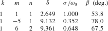
. The corresponding resonant frequencies (see table 2 in appendix B) are
 $$\begin{eqnarray}{\it\sigma}_{1,6,2}=0.648\,{\it\omega}_{0},\quad {\it\sigma}_{1,-5,1}=0.352\,{\it\omega}_{0}.\end{eqnarray}$$
In the rotating table reference frame, we must add to or subtract from these frequencies (depending on the sign of
 $m$
) the corresponding temporal frequency of the azimuthal
 $m$
mode, which is
 $m{\it\omega}_{0}$
. Therefore, the temporal frequency of the resonant modes, seen from the rotating table reference frame, is
 $$\begin{eqnarray}{\it\omega}_{\mathit{res}}=6{\it\omega}_{0}-{\it\sigma}_{1,6,2}=5{\it\omega}_{0}+{\it\sigma}_{1,-5,1}=5.352\,{\it\omega}_{0}.\end{eqnarray}$$
3. Base state flow
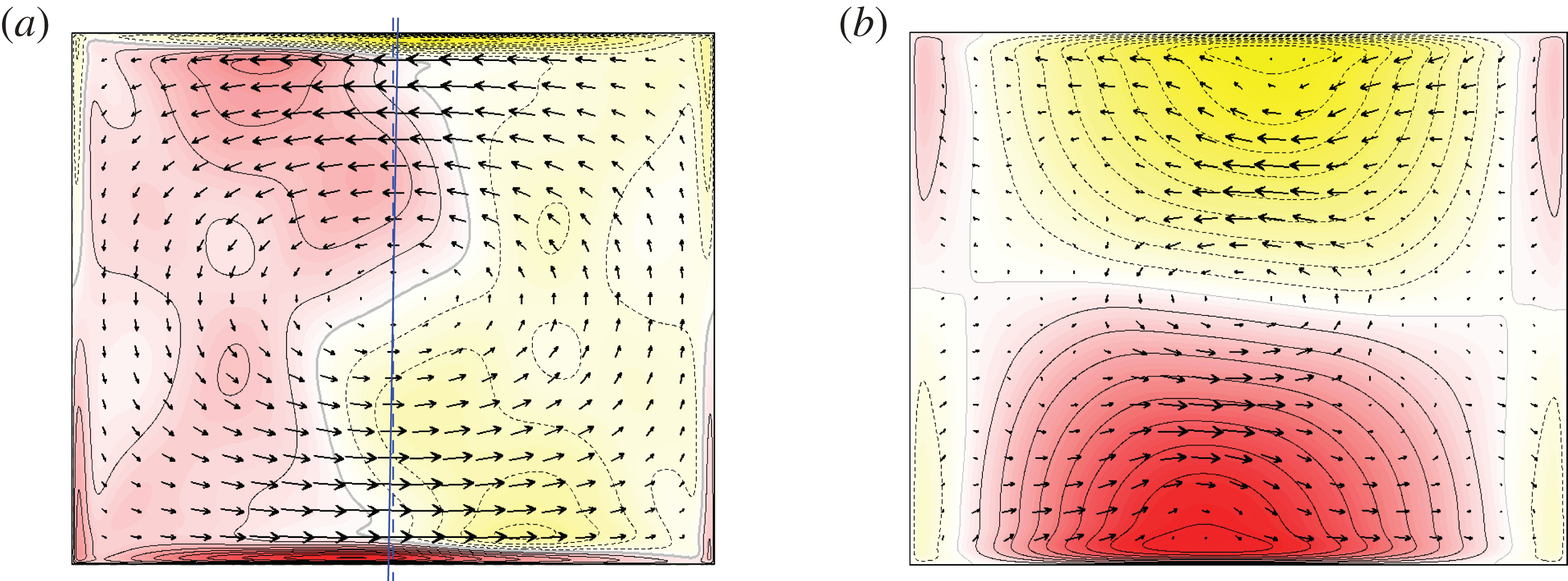
For sufficiently strong viscous dissipation in the system, the free Kelvin modes predicted by the triadic-resonance theory are damped, even at the exact resonance point, and the resultant flow is the base state. The base state is steady and inversion symmetric. It corresponds to the so-called spin-over mode in a cylinder (Greenspan Reference Greenspan1968), modified by viscous effects. Figure 2 shows the velocity field in two orthogonal meridional planes. Arrows for the in-plane velocities and contours for the normal velocity are plotted. The flow is dominated by a single vortex cell filling the whole domain. The velocity is large in the meridional plane where the angular velocity
 ${\it\omega}_{p}$
of the rotating table is located, corresponding to
 ${\it\theta}=90^{\circ }$
, as shown in figure 2(a). The dashed (blue) line coinciding with the axis of the cylinder indicates the cylinder rotation axis
 ${\it\omega}_{0}$
, and the solid (blue) line indicates the direction of
 ${\it\omega}_{p}$
; the angle between the two is
 ${\it\alpha}=1^{\circ }$
. Even such a small angle produces dramatic effects on the flow, generating the strong
 $m=1$
vortex indicated by arrows in figure 2(a). In the orthogonal plane
 ${\it\theta}=0$
, figure 2(b), the meridional velocity is almost zero (approximately 40 times smaller than in the
 ${\it\theta}=90^{\circ }$
plane), and the normal velocity contours show the orthogonal cut of the spin-over flow. Another feature of the base flow is the S-shape of the zero contour (thick grey line) in figure 2(a), which separates fluid rotating in opposite directions. This is consistent with visualizations of the core flow in experiments (Manasseh Reference Manasseh1992).
Base state flow at
 ${\it\omega}_{0}=4500$
,
 ${\it\omega}_{p}/{\it\omega}_{0}=-0.15253$
,
 ${\it\Gamma}=1.62$
and
 ${\it\alpha}=1^{\circ }$
, showing meridional sections at (a)
 ${\it\theta}=90^{\circ }$
and (b)
 ${\it\theta}=0$
; the arrows correspond to the in-plane meridional velocity
 $(u,w)$
and the contours/colour map correspond to the out-of-plane azimuthal velocity,
 $v$
. There are 10 positive (red, solid lines) and 10 negative (yellow, dashed lines) contours, equispaced in the range (a)
 $v\in [-200,200]$
and (b)
 $v\in [-650,650]$
. The arrows in (b) have been scaled by a factor of 10 relative to those in (a).

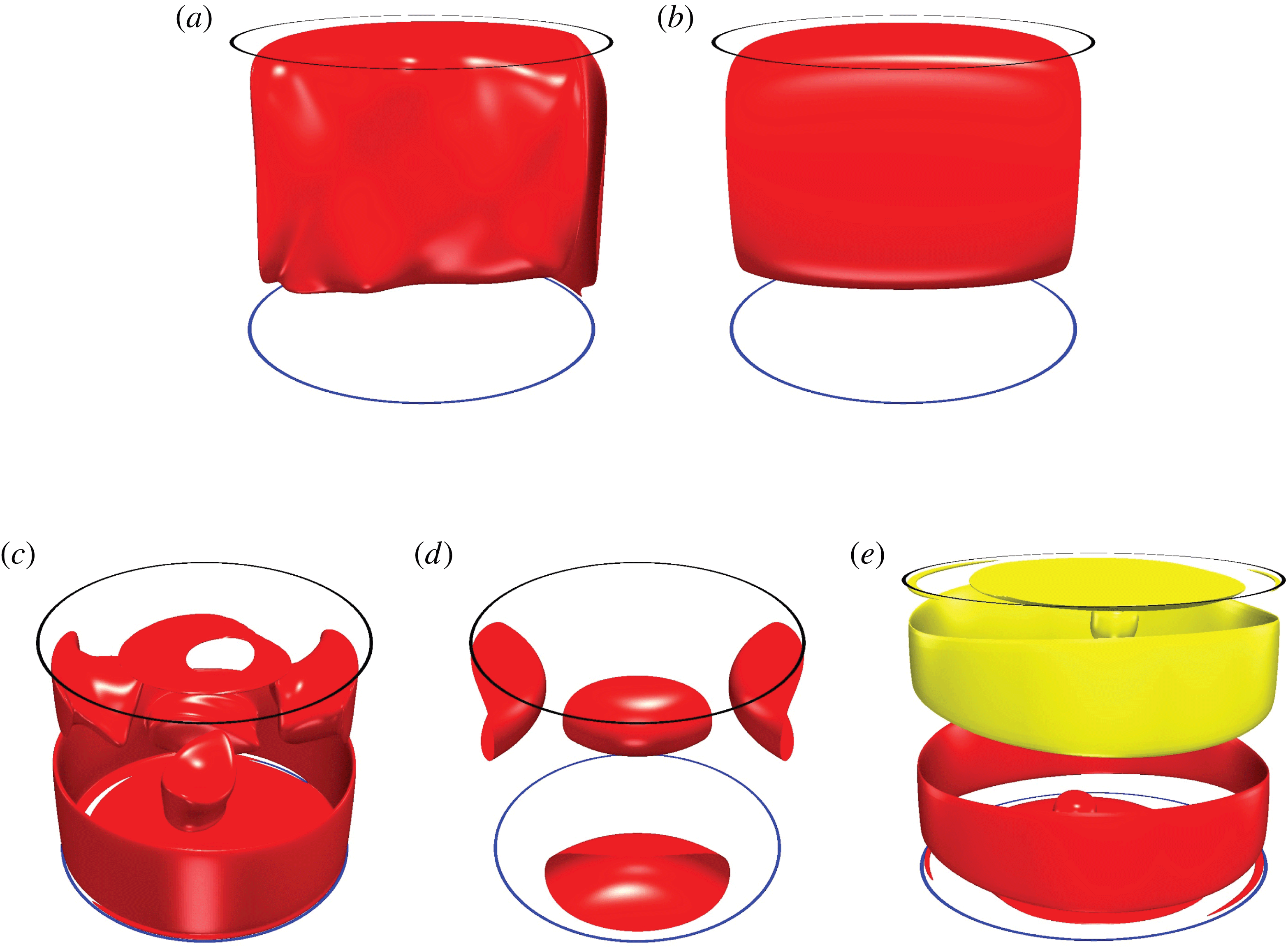
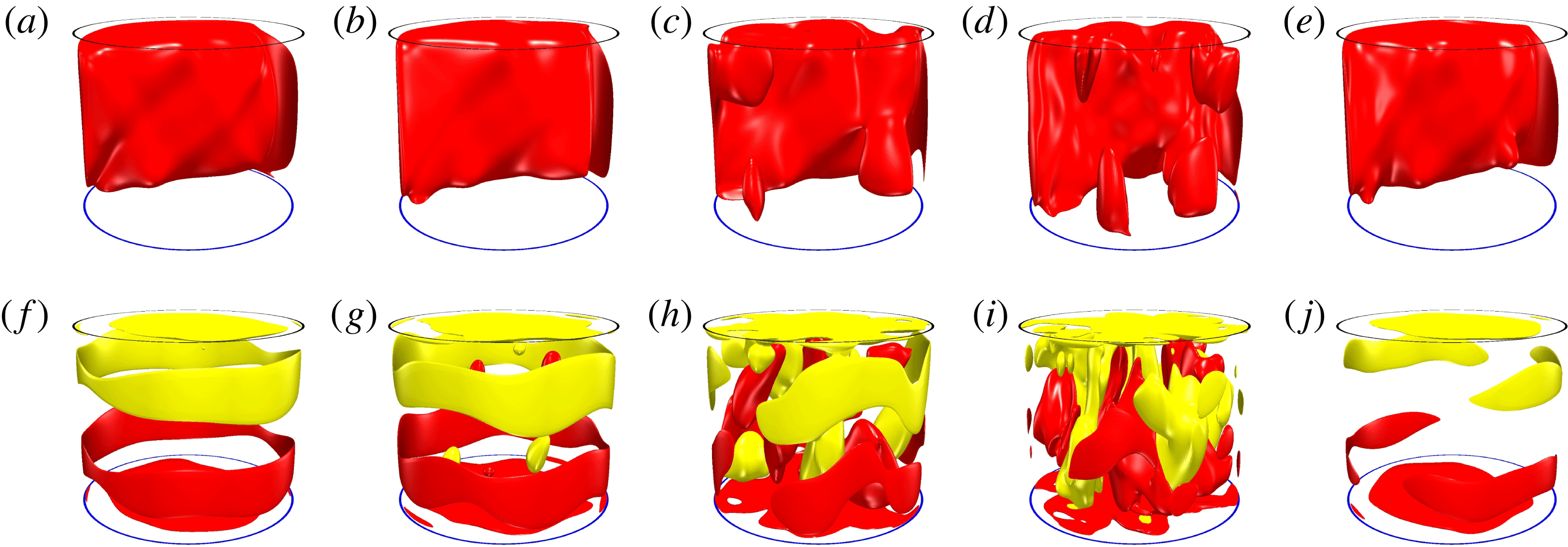
Figure 3(a) shows a three-dimensional rendering of an isosurface of the axial velocity at level
 $w=25$
, illustrating the basic state spin-over flow (the
 $w=-25$
isosurface is not shown, but is simply the inversion of the
 $w=25$
isosurface in the other half of the cylinder). The isosurface shows the presence of several folds. The folds go from the corners and reflect off the endwalls. These are essentially following the characteristics of the linearized inviscid approximation to the problem (they are not straight as the rotation of the fluid is perturbed away from solid-body rotation). The angle of the characteristics with the horizontal direction,
 ${\it\beta}$
, is given by the dispersion relation
 $2\cos {\it\beta}={\it\omega}_{f}$
, and for
 ${\it\omega}_{f}=1.18$
used in this example,
 ${\it\beta}\approx 53.9^{\circ }$
. Therefore, the folds correspond to inertial-wave beams emanating from the boundary layer at the corners. We can compare the base state with the
 $(1,1,1)$
Kelvin mode shown in figure 3(b). The shape is the same, but there are no inertial-wave beams, and the boundary layers are absent. These two features are due to viscosity acting in the boundary layers, and producing inertial-wave beams in addition to the Kelvin mode. The influence of the boundary layers is more evident when we plot an isosurface of the helicity of the base state in figure 3(c), at level
 $\mathscr{H}=5\times 10^{4}$
, and compare it with the helicity of the
 $(1,1,1)$
Kelvin mode shown in figure 3(d). The base state exhibits the four bulges shown in the Kelvin mode, substantially deformed, as well as a strong boundary layer and an ejection of helicity from the centre of the bottom endwall. Only the positive helicity is plotted for clarity; the negative is the inversion-symmetric image, and the inclination of the container has been changed in order to better see the interior. In figure 3(e) the helicity of the base state at levels
 $\mathscr{H}=\pm 1.5\times 10^{5}$
is shown. At this higher level (at approximately 4 % of the maximum value of
 $\mathscr{H}$
), the contribution to the helicity from the Kelvin mode is too weak to be seen, and the dominant features are helicity in the boundary layers and the ejection of helicity from the centre of the endwalls.
Isosurfaces of axial velocity for (a) the base state (same state as in figure 2) at level
 $w=25$
and (b) the
 $(1,1,1)$
Kelvin mode. Isosurfaces of the helicity for (c) the base state at levels
 $\mathscr{H}=5\times 10^{4}$
, (d) the
 $(1,1,1)$
Kelvin mode and (e) the base state at levels
 $\mathscr{H}=\pm 1.5\times 10^{5}$
.

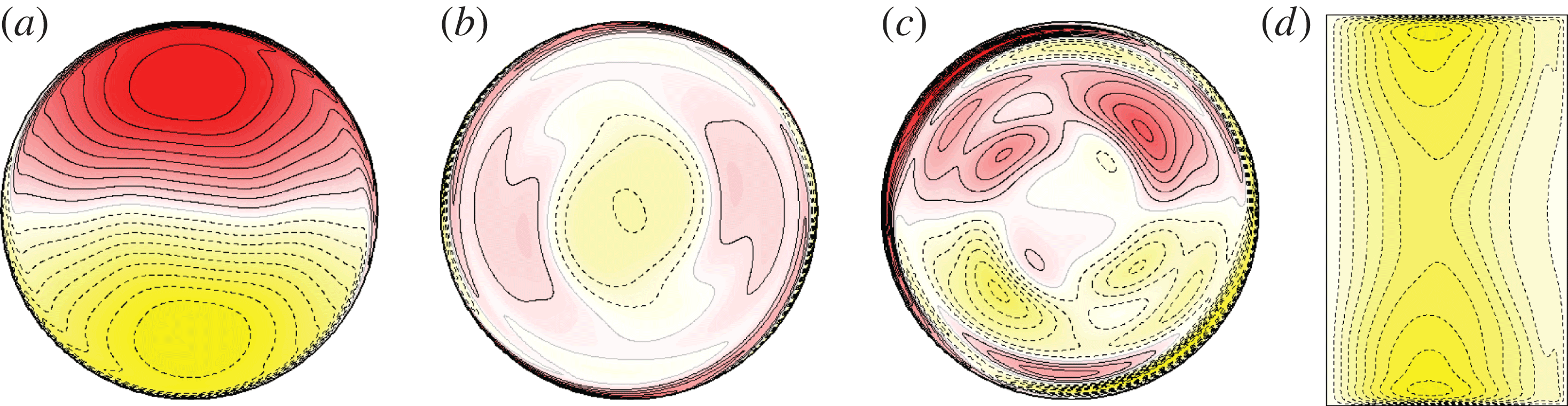
Base state at
 ${\it\omega}_{0}=4500$
,
 ${\it\omega}_{p}/{\it\omega}_{0}=-0.15253$
,
 ${\it\Gamma}=1.62$
and
 ${\it\alpha}=1^{\circ }$
; the horizontal sections are at the mid-plane and show contours of (a) axial velocity,
 $w$
, (b) axial vorticity,
 ${\it\zeta}$
, and (c) helicity,
 $\mathscr{H}$
. The contours in (d) are of the
 $m=0$
azimuthal Fourier component of the azimuthal velocity
 $v_{0}$
(deviation with respect to solid-body rotation) in a meridional plane, corresponding to the steady-streaming flow.

Variation with
 ${\it\omega}_{0}$
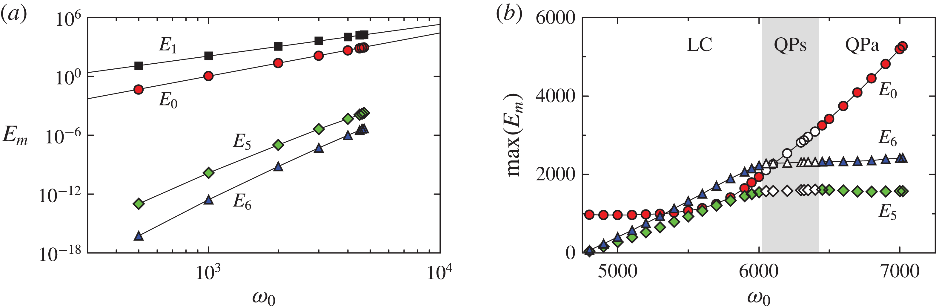
of (a) the primary modal kinetic energies of the basic state BS and (b) maxima in the modal kinetic energies of the time-periodic state LC and quasi-periodic states QPs and QPa (described in §§ 4.2 and 4.3), for
 ${\it\omega}_{p}/{\it\omega}_{0}=-0.15253$
,
 ${\it\Gamma}=1.62$
and
 ${\it\alpha}=1^{\circ }$
.

In figure 4(a–c), contours of axial velocity
 $w$
, axial vorticity
 ${\it\zeta}$
and helicity
 $\mathscr{H}$
are shown at the mid-plane
 $z=0$
. The contours of
 $w$
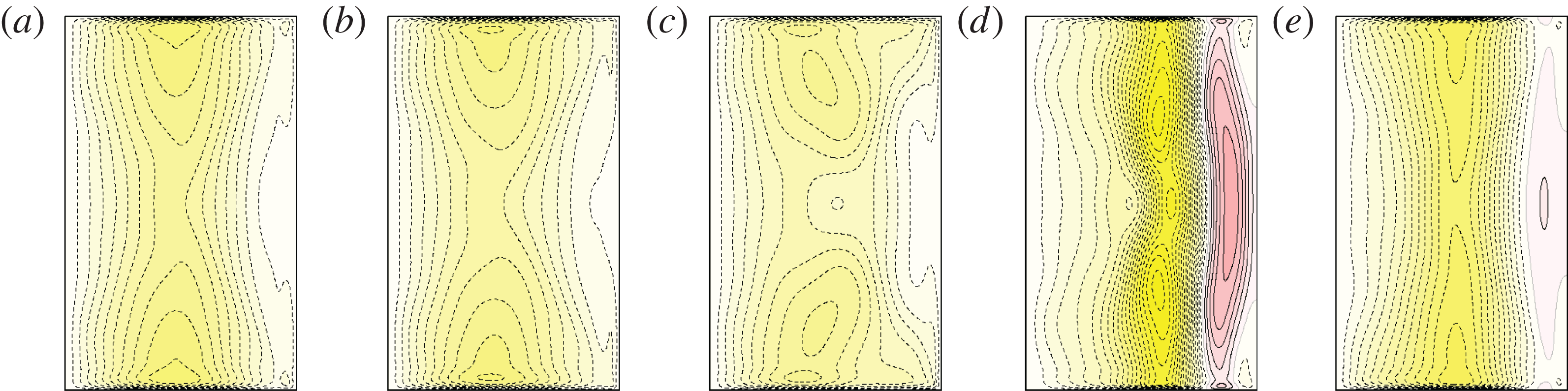
show a horizontal section of the forced spin-over flow. The axial vorticity is very weak in the bulk of the flow, and is concentrated mainly at the wall boundary layer. The contours of helicity show that the vortical structure of the spin-over flow is complicated: both the upward and the downward parts of the vortex cell have a pair of helicity columns inside, although this helical motion is much smaller than the helicity in the wall boundary layer. Viscosity and nonlinearity result in an axisymmetric azimuthal mean flow, the steady-streaming flow, shown in figure 4(d), consisting of contours of the
 $m=0$
azimuthal Fourier component of the azimuthal velocity,
 $v_{0}$
. These contours have small variations in the axial direction, except near the endwalls, and this streaming flow is often referred to as the geostrophic mode (Greenspan Reference Greenspan1968). However, the streaming flow has departures from geostrophic (
 $\partial v_{0}/\partial z\neq 0$
) due to the inertial-wave beams emanating from the corners: the angles of the
 $v_{0}=\text{constant}$
lines in figure 4(d) close to the corners are the same as the inertial-wave beams shown in figure 3(a).
We can compare figure 4 with the
 $(1,1,1)$
Kelvin mode: for this Kelvin mode, the axial vorticity
 ${\it\zeta}$
and helicity
 $\mathscr{H}$
are zero at the mid-plane, so all features displayed in figure 4(b,c) are due to nonlinearities and boundary layer effects. The same is true with the streaming flow, which is also absent in the
 $(1,1,1)$
Kelvin mode. The wrinkles in the
 $w$
contours, especially about the zero contour, are due to the inertial-wave beams described earlier. The presence of the inertial-wave beams is also evident in the streaming flow shown in figure 4(d), where they emanate from the corners at the same angle as is evident in figure 3(a). The presence of the beams means that the streaming flow is not geostrophic, i.e. the beams impart non-negligible axial gradients to the streaming flow throughout the flow.
4. Instabilities inside the resonance
We now consider the fate of the basic state at the predicted first resonance as viscous effects are reduced. Specifically, we fix
 ${\it\alpha}=1^{\circ }$
and
 ${\it\Gamma}=1.62$
, for which the spin-over
 $m=1$
mode has a primary resonance at
 ${\it\omega}_{f}=1.18$
(Lagrange et al.
Reference Lagrange, Meunier, Nadal and Eloy2011). These fixed values of
 ${\it\alpha}$
and
 ${\it\omega}_{f}$
correspond to a fixed Poincaré number
 ${\it\omega}_{p}/{\it\omega}_{0}=-0.15253$
. We now increase
 ${\it\omega}_{0}$
(and therefore
 ${\it\omega}_{p}$
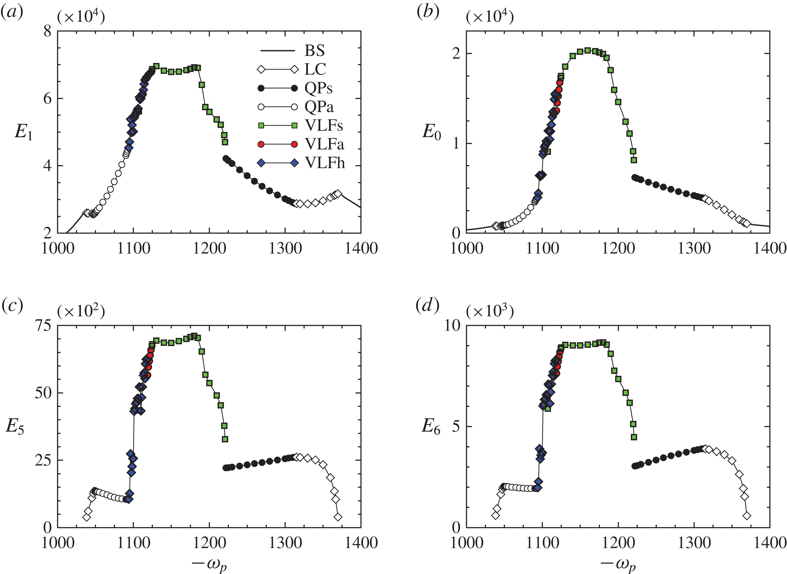
) from the viscous dominated values where the basic state is the unique stable solution. Figure 5(a) shows the development of the modal kinetic energies of the base state. These are
 $E_{1}$
, the modal energy of the azimuthal wavenumber
 $m=1$
forced spin-over component of the flow,
 $E_{0}$
, the modal energy of the axisymmetric streaming (geostrophic) component (the solid-body rotation of the cylinder has been subtracted), and
 $E_{5}$
and
 $E_{6}$
. For the basic state, the
 $m=5$
and
 $m=6$
components are simply harmonics of the forced
 $m=1$
mode, as are all of the
 $m\neq 0$
components. We include them in the figure as they are involved in the instability of the base state. The energies
 $E_{0}$
and
 $E_{1}$
follow the power laws
 $E_{0}\propto {\it\omega}_{0}^{4.40}$
and
 $E_{1}\propto {\it\omega}_{0}^{3.23}$
, represented by solid lines in the figure. The energy
 $E_{0}$
grows faster than
 $E_{1}$
, and on extrapolating they would eventually become equal at
 ${\it\omega}_{0}\sim 57\,500$
; however, the base state becomes unstable well before this value.
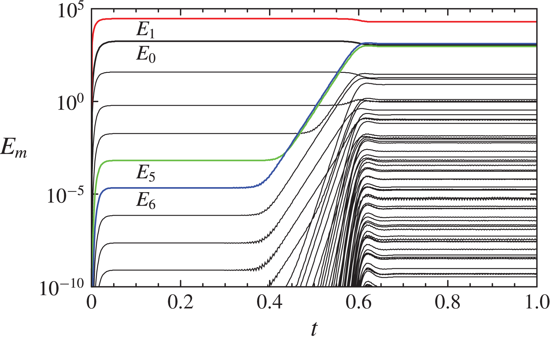
Time series of the modal kinetic energies,
 $E_{m}$
, for
 ${\it\omega}_{0}=5500$
,
 ${\it\omega}_{p}/{\it\omega}_{0}=-0.15253$
,
 ${\it\Gamma}=1.62$
and
 ${\it\alpha}=1^{\circ }$
, following an impulsive start of the table rotation with the cylinder initially in solid-body rotation.

4.1. The symmetric limit cycle
The first bifurcation of the base state as
 ${\it\omega}_{0}$
is increased inside the resonance region is to a periodic solution, a limit cycle LC. On comparing
 $E_{5}$
and
 $E_{6}$
for the base state in figure 5(a) with the maxima of the corresponding energies of the time-periodic LC solution in figure 5(b), we observe that these energies grow by more than six orders of magnitude over a very small range in
 ${\it\omega}_{0}$
, growing to be of the same order of magnitude as the
 $m=0$
streaming flow, but still an order of magnitude smaller than the
 $m=1$
spin-over flow forced by the precession of the cylinder;
 $E_{1}$
is not included in the figure so that the details of the variations in the other energies can be appreciated in this linear–linear plot. Figure 6 shows the time series of the modal azimuthal kinetic energies for a case where at
 $t=0$
the cylinder flow is in solid-body rotation, corresponding to
 ${\it\omega}_{0}=5500$
, with
 ${\it\Gamma}=1.62$
and
 ${\it\alpha}=1^{\circ }$
, and the table is impulsively set to rotate such that
 ${\it\omega}_{p}/{\it\omega}_{0}=-0.15253$
. It shows that by
 $t\approx 0.05$
, the system has spun up to the
 $m=1$
BS described earlier for lower
 ${\it\omega}_{0}$
, which appears to be stable with no discernible variations in the modal energies for over a third of a viscous time. However, a little later on,
 $E_{6}$
is seen to be growing exponentially fast, along with other
 $E_{m}$
. Extrapolating the growth in
 $E_{6}$
back in time, we see that this exponential growth begins from numerical noise levels (
 ${\sim}10^{-20}$
) from approximately the time the BS state has been spun up. We do not see evidence of this growth until it grows to the level of
 $E_{6}$
corresponding to the sixth harmonic of the
 $m=1$
BS. The energy
 $E_{5}$
starts to grow exponentially when
 $E_{6}$
reaches the level of the fifth harmonic of BS, and they both grow hand-in-hand, with
 $E_{5}$
always slightly smaller than
 $E_{6}$
, until they reach the level of
 $E_{0}$
, at which point they saturate nonlinearly, primarily by extracting energy from
 $E_{0}$
and
 $E_{1}$
. The Kelvin modes with azimuthal wavenumbers
 $m=5$
and
 $m=6$
are the two that are predicted to be excited via a triadic resonance with the forced
 $m=1$
spin-over flow (Lagrange et al.
Reference Lagrange, Meunier, Nadal and Eloy2011). The modal energies
 $E_{6}$
and
 $E_{5}$
grow linearly with
 ${\it\omega}_{0}$
, and so the corresponding velocity amplitudes grow proportional to
 ${\it\omega}_{0}^{0.5}$
. This behaviour is typical of a supercritical Hopf bifurcation, in which the resonant modes
 $m=5$
and 6 come into play. A linear fit to the LC energies in figure 5(b) gives
 ${\it\omega}_{0}\approx 4777$
as the bifurcation point value; P. Meunier (private communication, 2015) has used the reduced model from Lagrange et al. (Reference Lagrange, Meunier, Nadal and Eloy2011) and found the critical value to be
 ${\it\omega}_{0}\approx 4956$
, which is less than 4 % different from the results using the full Navier–Stokes equations. Below this critical
 ${\it\omega}_{0}$
value, viscous effects are strong and the resonance does not manifest itself. As
 $E_{6}$
and
 $E_{5}$
become larger, the associated eigenmodes begin to have a non-negligible interaction with the viscous boundary layers, resulting in a contribution to the
 $m=0$
streaming flow, and
 $E_{0}$
is seen to begin to grow rapidly for
 ${\it\omega}_{0}\gtrsim 5800$
; this leads to an instability of LC. It is worth mentioning that the energies of the other azimuthal Fourier modes are at least two orders of magnitude smaller than for modes
 $m=0$
, 1, 5 and 6.
For LC at
 ${\it\omega}_{0}=5500$
,
 ${\it\omega}_{p}/{\it\omega}_{0}=-0.15253$
,
 ${\it\Gamma}=1.62$
and
 ${\it\alpha}=1^{\circ }$
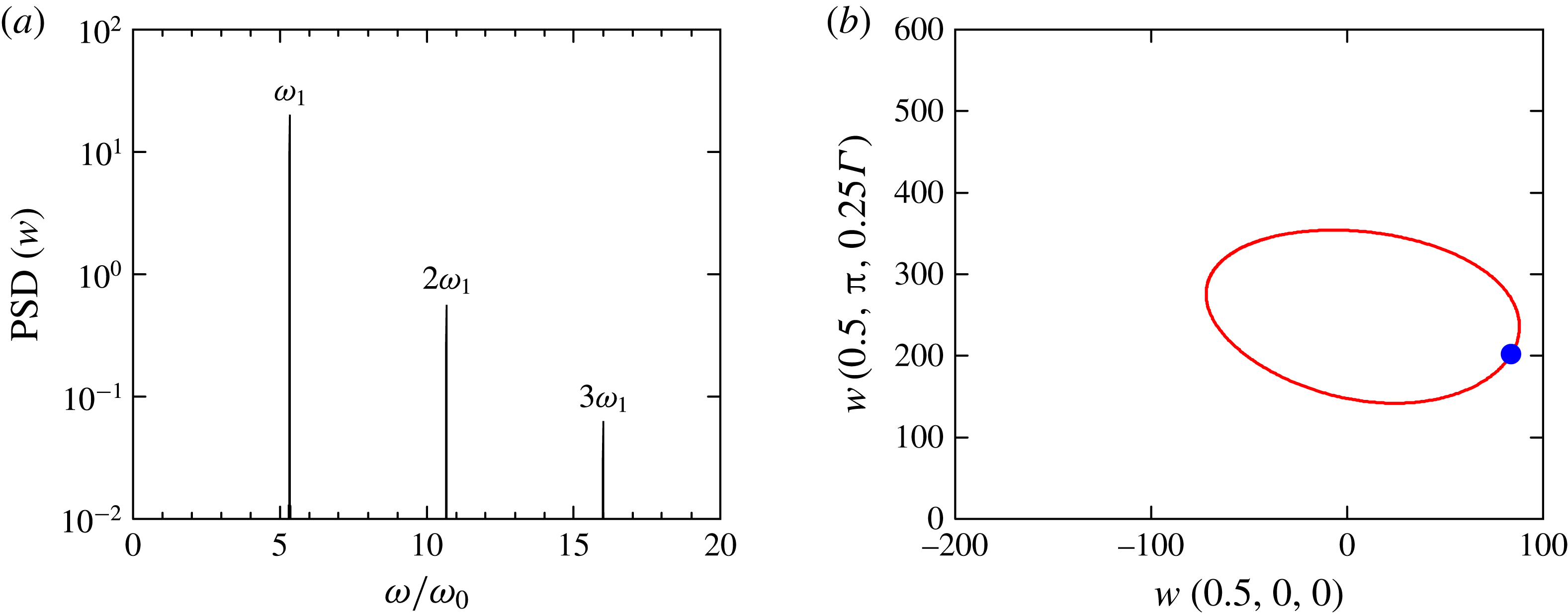
, (a) shows the power spectral density of
 $w(0.5,0,0)$
and (b) shows the phase portrait of
 $w$
at
 $(0.5,0,0)$
and
 $(0.5,{\rm\pi},-0.25{\it\Gamma})$
; the Poincaré section corresponds to
 $w(0.5,{\rm\pi},-0.25{\it\Gamma})=97$
.

Figure 7(a) shows the power spectral density (PSD) of the time series of the axial velocity
 $w$
at the point
 $(0.5,0,0)$
of LC at
 ${\it\omega}_{0}=5500$
,
 ${\it\omega}_{p}/{\it\omega}_{0}=-0.15253$
,
 ${\it\Gamma}=1.62$
and
 ${\it\alpha}=1^{\circ }$
. It consists of a single frequency
 ${\it\omega}_{1}=2.93\times 10^{4}$
and its multiples. The period of this solution is
 ${\it\tau}_{1}=2{\rm\pi}/{\it\omega}_{1}\approx 2.14\times 10^{-4}$
, corresponding to approximately 5.3 oscillations for every rotation of the cylinder. It should be noted that this corresponds to
 ${\it\omega}_{1}/{\it\omega}_{0}\approx 5.327$
, which is in very good agreement with
 ${\it\omega}_{\mathit{res}}=5.352$
from the linear triadic-resonance theory (2.25); the difference is less than 0.5 %. Therefore, we can say that the Hopf bifurcation is induced by the triadic resonance at the present parameter values. Figure 7(b) shows a two-dimensional projection of the LC phase portrait, obtained using the axial velocity at two points in the flow,
 $w(0.5,0,0)$
and
 $w(0.5,{\rm\pi},-0.25{\it\Gamma})$
. The (blue) symbol in the figure is the Poincaré section of the limit cycle at
 $w(0.5,{\rm\pi},-0.25{\it\Gamma})=97$
. We will use the same phase portrait and Poincaré section later in order to characterize more complex solutions. This periodic solution is not a rotating wave because the base state from which it bifurcates is not axisymmetric. However, the modal energies have very small variation in time, similar to a rotating wave that has constant modal energies; the variation of the energies is approximately one part in a million. This is because the excited modes
 $m=5$
and
 $m=6$
are essentially rotating waves, while the
 $m=1$
mode (the underlying base state) is pinned to the tilted precession angle direction and does not rotate, as will be shown below.
For LC at
 ${\it\omega}_{0}=5500$
,
 ${\it\omega}_{p}/{\it\omega}_{0}=-0.15253$
,
 ${\it\Gamma}=1.62$
and
 ${\it\alpha}=1^{\circ }$
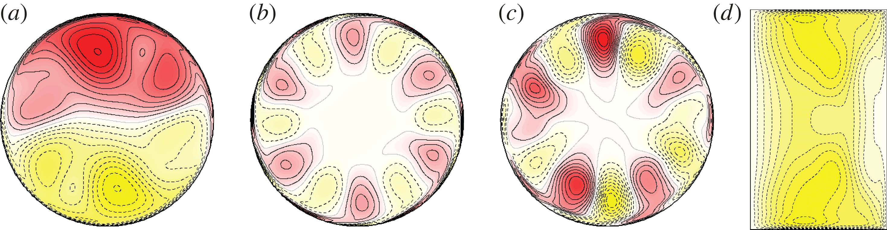
, the mid-plane horizontal sections show contours of (a) axial velocity, (b) axial vorticity and (c) helicity. The contours in (d) show the streaming flow
 $v_{0}$
in a meridional
 $(r,z)$
plane (
 ${\it\theta}$
is arbitrary since
 $v_{0}$
is axisymmetric, and the left boundary of the figure is the cylinder axis
 $r=0$
). See online movies for animations over one period.

The
 $\mathscr{J}$
-symmetric LC at
 ${\it\omega}_{0}=5500$
is illustrated in figure 8, which shows contours of the axial velocity, axial vorticity and helicity at the mid-plane
 $z=0$
, and of the
 $v_{0}$
streaming flow in a meridional plane. In the mid-plane
 $z=0$
the inversion symmetry manifests itself as a rotational symmetry of
 $180^{\circ }$
. The inversion symmetry of LC can also be verified by directly computing the symmetry parameter of this solution; it is
 $\mathscr{S}\approx 3\times 10^{-9}$
, which is essentially numerical noise about zero.
On comparing the
 $w$
contours of LC with the base state in figure 4(a), we observe that the forced spin-over flow is still the dominant feature, and it remains essentially steady. The temporal dependence corresponds to superimposed perturbations travelling anticlockwise (as seen from the top lid) in the azimuthal direction (see the supplementary movies available at http://dx.doi.org/10.1017/jfm.2015.524). Figure 8(b) shows contours of axial vorticity
 ${\it\zeta}$
at the mid-plane. As discussed in § 2.1, due to the
 $\mathscr{J}$
-symmetry of LC, the odd azimuthal Fourier modes of
 ${\it\zeta}$
at the mid-plane are zero, and this figure does not have any contribution from the
 $m=1$
azimuthal component. From the accompanying online movie, it is evident that the
 $m=6$
mode is travelling anticlockwise at exactly
 ${\it\omega}_{1}/6=4890$
, approximately 10 % smaller than
 ${\it\omega}_{0}$
. In fact,
 ${\it\zeta}$
at the mid-plane is not a pure rotating wave since there are very small modulations in
 ${\it\zeta}$
during the period, due to the effects of the small but non-zero even modes (in particular
 $m=2$
and
 $m=4$
). Figure 8(c) shows contours of helicity
 $\mathscr{H}$
at the mid-plane. As discussed in § 2.1, due to the
 $\mathscr{J}$
-symmetry of LC, the even azimuthal Fourier modes of
 $\mathscr{H}$
at the mid-plane are zero, and this figure does not have any contribution from the
 $m=0$
and
 $m=6$
modes. The
 $m=5$
contribution is clearly visible, and there is also a strong contribution from
 $m=1$
. The accompanying online movie shows the
 $m=5$
azimuthal rotation over the fixed
 $m=1$
component.
It is also interesting to note that the positive
 ${\it\zeta}$
values in figure 8(b) are larger than the negative values, due to the presence of the streaming flow. Figure 8(d) shows contours of the
 $m=0$
component of the azimuthal velocity,
 $v_{0}$
, on a meridional plane. The deviation of the azimuthal velocity with respect to the solid-body rotation has a well-defined sign (negative), therefore the bulk of the fluid has a counterclockwise azimuthal rotation on average; this is called the streaming flow. We can compare the
 $v_{0}$
streaming flow of LC at
 ${\it\omega}_{0}=5500$
in figure 8(d) with the
 $v_{0}$
streaming flow of the base state at
 ${\it\omega}_{0}=4500$
in figure 4(d). They look similar, but for LC
 $v_{0}$
has developed an indentation in the mid-plane and an equatorial band that is almost stagnant relative to the sidewall motion; these are the effects of the
 $m=5$
and 6 resonant modes. Although the LC solution is periodic, its streaming flow is essentially steady: it shows very small variations in time that cannot be appreciated in a movie of the
 $v_{0}$
contours. It should be mentioned that the
 $(1,-5,1)$
and
 $(1,6,2)$
Kelvin modes that participate in the triadic resonance leading to the LC state have associated wave beam angles that are different from that of the
 $(1,1,1)$
forced Kelvin mode that is responsible for BS; they are respectively
 $78.0^{\circ }$
and
 $67.5^{\circ }$
, compared with
 $53.8^{\circ }$
(see table 2).
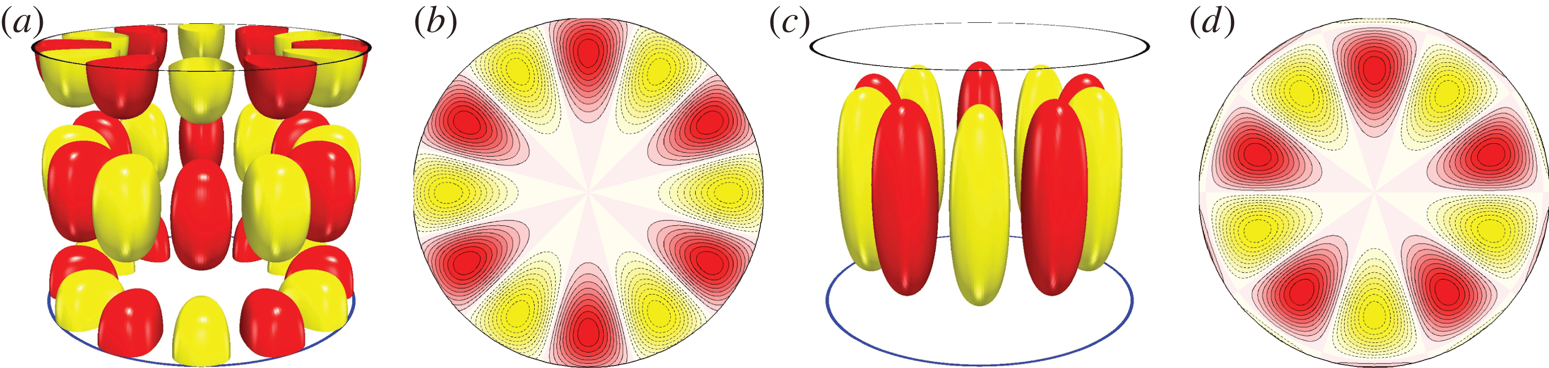
(a) Isosurfaces and (b) contours on the mid-plane of the axial vorticity of the
 $(1,6,2)$
inviscid Kelvin mode, and (c) isosurfaces and (d) contours on the mid-plane of the axial velocity of the
 $(1,-5,1)$
inviscid Kelvin mode.

We can compare the LC solution with the pure Kelvin modes that are part of the triadic-resonance mechanism. Figure 9 shows an isosurface and contours on the mid-plane for the axial vorticity of the
 $(1,6,2)$
Kelvin mode and for the axial velocity of the
 $(1,-5,1)$
Kelvin mode. We have selected these plots because of the three variables (
 $w$
,
 ${\it\zeta}$
and
 $\mathscr{H}$
) we have shown for BS and LC; they are the only ones that do not vanish at the mid-plane for these Kelvin modes (see the analytic expressions in (2.22) and (B 8)). The 3D isosurfaces shown in figure 9(a,c) display the spatial structure of these modes, and illustrate the significance of the three integers
 $(k,m,n)$
that are directly related to the number of zeros of the Kelvin modes in the radial, azimuthal and axial directions respectively. The resemblance between the contours at mid-plane of
 ${\it\zeta}$
for the
 $(1,6,2)$
Kelvin mode (figure 9
b) and the LC solution (figure 8
b) is very strong. It may come as a surprise that the contours at mid-plane of
 $w$
for the
 $(1,-5,1)$
Kelvin mode (figure 9
d) and
 $\mathscr{H}$
for the LC solution (figure 8
c) are also very similar. However, one should note that there is not a direct relationship between the azimuthal
 $m$
Fourier mode of the solution to the full Navier–Stokes equations and the Kelvin eigenmode with azimuthal wavenumber
 $m$
. The Navier–Stokes solutions are intrinsically nonlinear, and any particular azimuthal Fourier mode contains information of all the azimuthal Fourier modes of the solution via interaction through the nonlinear advection term. For example, the helicity
 $\mathscr{H}$
is zero at the mid-plane for the
 $(1,-5,1)$
Kelvin mode, while the
 $m=5$
azimuthal Fourier component of
 $\mathscr{H}$
(which is a quadratic, i.e. nonlinear variable) of the LC solution, has contributions from the non-zero product
 $w_{5}{\it\zeta}_{0}$
(and others) at the mid-plane. This particular term of interaction between the
 $m=5$
azimuthal Fourier mode,
 $w_{5}$
, and the
 $m=0$
streaming flow,
 ${\it\zeta}_{0}$
, explains the strong resemblance between figures 9(d) and 8(c). This points to a warning that one must be careful when comparing solutions of the full Navier–Stokes equations with the Kelvin modes.
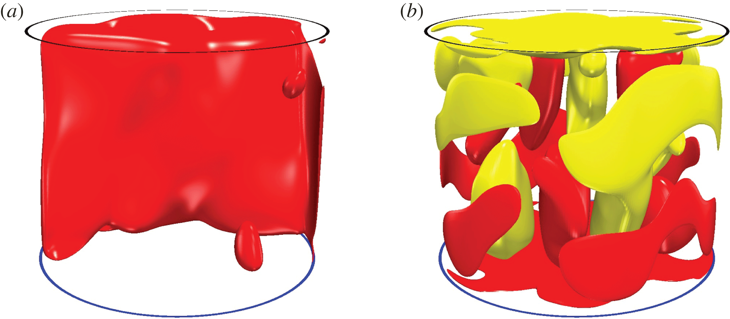
Isosurfaces of (a) the axial velocity at level
 $w=25$
and (b) the helicity at levels
 $\mathscr{H}=\pm 3\times 10^{5}$
of the LC at
 ${\it\omega}_{0}=5500$
,
 ${\it\omega}_{p}/{\it\omega}_{0}=-0.15253$
,
 ${\it\Gamma}=1.62$
and
 ${\it\alpha}=1^{\circ }$
. See online movies for animations over one period.

Power spectral density of QPs at
 ${\it\omega}_{0}=6300$
,
 ${\it\omega}_{p}/{\it\omega}_{0}=-0.15253$
,
 ${\it\Gamma}=1.62$
and
 ${\it\alpha}=1^{\circ }$
.

Figure 10 shows an isosurface of the axial velocity
 $w$
and the helicity
 $\mathscr{H}$
of LC at
 ${\it\omega}_{0}=5500$
, which can be directly compared with the corresponding isosurfaces of BS in figure 2(a,e). The isosurfaces of
 $w$
for BS and LC are similar, indicating that the spin-over flow, forced by the slight inclination of the cylinder axis, is a dominant characteristic of both flows. In the LC solution, the isosurface of
 $w$
is more distorted, and the signature of the inertial-wave beams is more complicated due to the presence of the resonant modes with
 $m=5$
and 6, whose angles of propagation,
 ${\it\beta}$
, of their respective inertial-wave beams are different (see table 2). The
 $\mathscr{H}$
isosurface for LC is much more complex than that corresponding to BS, and the presence of the
 $m=5$
and 6 resonant modes results in a complex interior pattern, absent in BS. The accompanying online movies clearly show the spatial complexity of this time-periodic flow.
4.2. The symmetric quasiperiodic flow
On increasing
 ${\it\omega}_{0}$
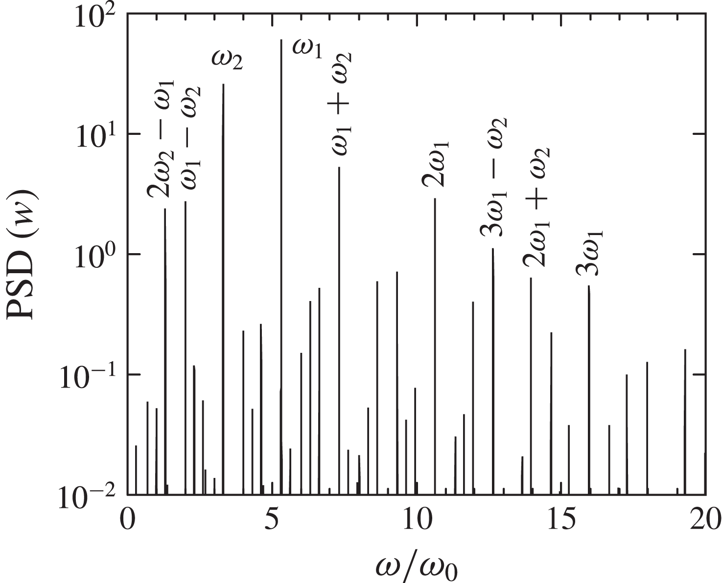
, the periodic LC loses stability, as shown in figure 5(b), to a quasiperiodic solution. Figure 11 shows the PSD of the quasiperiodic state at
 ${\it\omega}_{0}=6300$
, consisting of two well-defined frequencies,
 ${\it\omega}_{1}$
and
 ${\it\omega}_{2}$
, and their linear combinations. This should be compared with the PSD of LC at
 ${\it\omega}_{0}=5500$
in figure 7(a), consisting of a single frequency
 ${\it\omega}_{1}$
and its harmonics. The instability is due to a secondary Hopf bifurcation, also known as a Neimark–Sacker bifurcation (Kuznetsov Reference Kuznetsov2004). Specifically,
 ${\it\omega}_{1}=3.352\times 10^{4}$
and
 ${\it\omega}_{2}=2.090\times 10^{4}$
; they are in an approximate ratio
 ${\it\omega}_{2}/{\it\omega}_{1}\approx 5/8$
. The quasiperiodic state is also
 $\mathscr{J}$
-symmetric, verified by directly computing the symmetry parameter
 $\mathscr{S}$
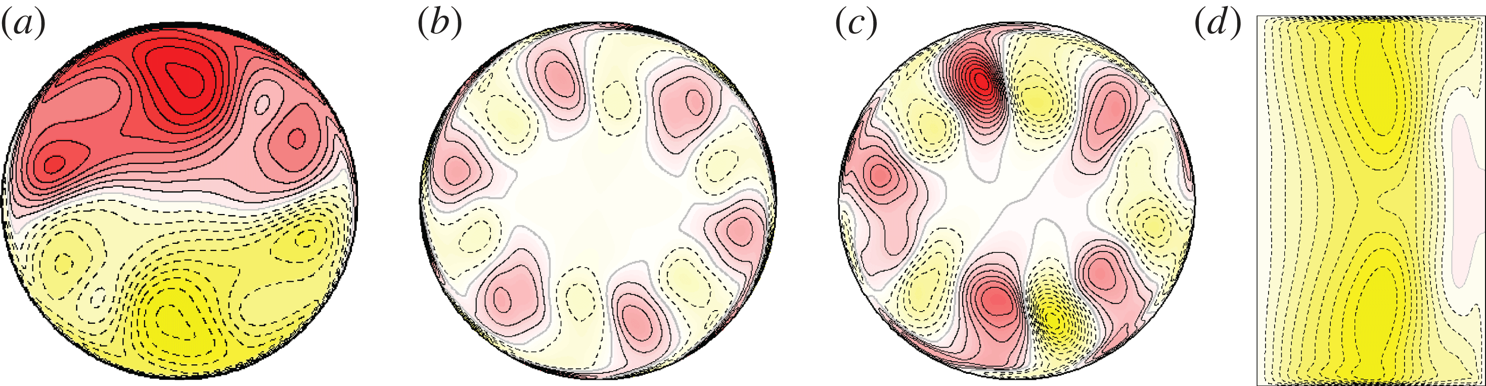
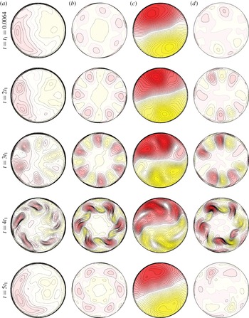
, and shall be referred to as QPs. The symmetry can also be observed from contours of any variable at the mid-plane, as illustrated in figure 12(a–c), showing contours of axial velocity, axial vorticity and helicity; the inversion symmetry manifests itself as a rotational symmetry of
 $180^{\circ }$
. For LC, the axial vorticity
 ${\it\zeta}$
at the mid-plane (figure 8
b) was a rotating wave and the streaming flow (figure 8
d) was steady and negative throughout the whole cylinder; both with minuscule modulations. For QPs,
 ${\it\zeta}$
has significant variations due to the second frequency, the streaming flow
 $v_{0}$
is no longer steady, and has an equatorial belt with positive
 $v_{0}$
(see figure 12 and the corresponding online movies). The time variations of
 ${\it\zeta}$
, apart from the azimuthal translations, are not oscillations in intensity, but an oscillation in the radial direction. These are correlated with radial variations in time of the streaming flow. This radial oscillation has a frequency
 ${\it\omega}_{2}$
. The modal energies
 $E_{5}$
and
 $E_{6}$
do not change with increasing
 ${\it\omega}_{0}$
, while
 $E_{0}$
, which includes the streaming flow energy, increases linearly with
 ${\it\omega}_{0}$
, as shown in figure 5(b). Increase of the streaming flow energy results in additional bifurcations when
 ${\it\omega}_{0}$
is increased above 6400.
The QPs at
 ${\it\omega}_{0}=6300$
,
 ${\it\omega}_{p}/{\it\omega}_{0}=-0.15253$
,
 ${\it\Gamma}=1.62$
and
 ${\it\alpha}=1^{\circ }$
; the mid-plane horizontal sections show contours of (a) axial velocity, (b) axial vorticity and (c) helicity. The contours in (d) show the streaming flow
 $v_{0}$
in a meridional
 $(r,z)$
plane. See online movies for animations over one period.

For QPs at
 ${\it\Gamma}=1.62$
,
 ${\it\alpha}=1^{\circ }$
,
 ${\it\omega}_{p}/{\it\omega}_{0}=-0.15253$
and
 ${\it\omega}_{0}=6300$
, (a) shows a phase portrait of
 $w$
at
 $(0.5,0,0)$
and
 $(0.5,{\rm\pi},-0.25{\it\Gamma})$
; the Poincaré section corresponds to
 $w(0.5,{\rm\pi},-0.25{\it\Gamma})=40$
; (b) shows the phase portrait of the energies
 $E_{0}$
and
 $E_{6}$
; the Poincaré section corresponds to
 $E_{5}=1578$
.

Phase portraits and Poincaré sections of the stable QPa and unstable QPs at
 ${\it\Gamma}=1.62$
,
 ${\it\alpha}=1^{\circ }$
,
 ${\it\omega}_{p}/{\it\omega}_{0}=-0.15253$
and
 ${\it\omega}_{0}=6500$
. The Poincaré sections correspond to
 $w(0.5,{\rm\pi},-0.25{\it\Gamma})=50$
in (a) and (b), to
 $E_{5}=1580$
in (c) and to
 $E_{5}=1610$
in (d).

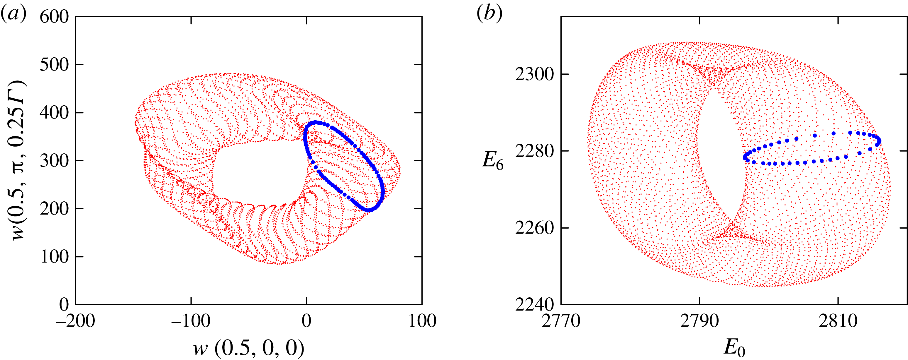
Figure 13(a) shows a two-dimensional projection of the QPs phase portrait, the same projection that was used for LC in figure 7(b), showing the two-torus nature of QPs. The Poincaré section at
 $w(0.5,{\rm\pi},-0.25{\it\Gamma})=40$
is shown as the solid (blue) curve. Figure 13(b) shows a different phase portrait and Poincaré section, using the modal energies
 $E_{0}$
and
 $E_{6}$
.
4.3. Torus doubling: breaking
 $\mathscr{J}$
-symmetry

On increasing
 ${\it\omega}_{0}$
above
 $6400$
, QPs loses stability to a very similar solution, QPa, which breaks the
 $\mathscr{J}$
-symmetry. Figure 5(a) shows that the energies of the primary modes
 $m=0$
, 1, 5 and 6 vary smoothly with
 ${\it\omega}_{0}$
and do not indicate the presence of a transition or bifurcation. However, the phase portrait of QPa at
 ${\it\omega}_{0}=6500$
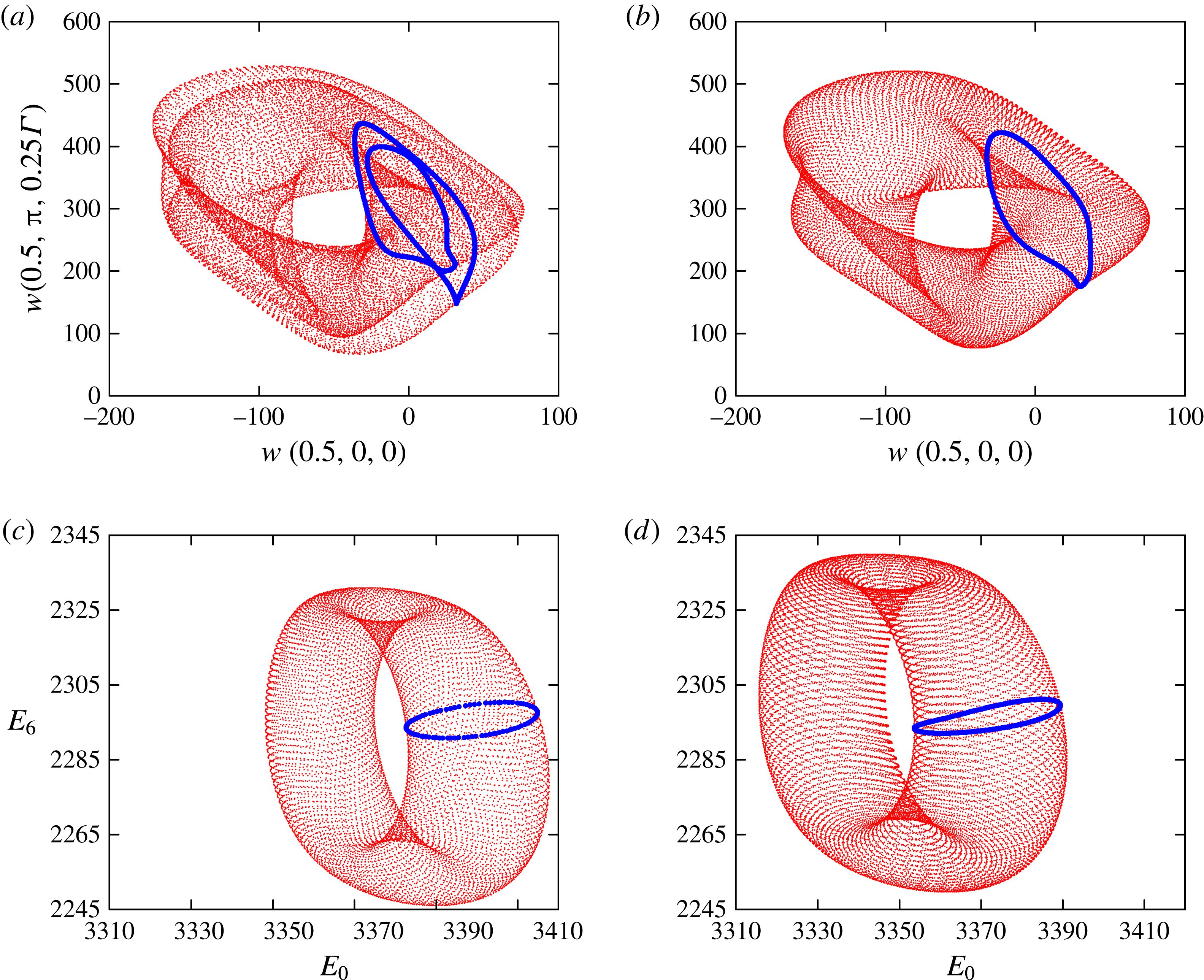
shown in figure 14(a) reveals a dramatic change: the two-torus QPs has undergone a torus-doubling bifurcation. This is clearly evident from the Poincaré section of QPa which shows an invariant circle that has doubled in comparison with the same Poincaré section of QPs (see figure 13). The symmetry parameter
 $\mathscr{S}$
of this new branch of solutions is of order one, indicating that the
 $\mathscr{J}$
-symmetry is broken, i.e. the QPa solutions are not point-wise
 $\mathscr{J}$
-symmetric (a point-wise
 $\mathscr{J}$
-symmetric flow is one that at any instant in time is
 $\mathscr{J}$
-invariant). By restricting the numerical simulations to the
 $\mathscr{J}$
-invariant subspace, the QPs branch can be continued numerically up to higher values of
 ${\it\omega}_{0}$
beyond the bifurcation. Figure 14(b) shows the phase portrait of the unstable QPs computed at
 ${\it\omega}_{0}=6500$
, the same value of
 ${\it\omega}_{0}$
used for QPa in figure 14(a). The doubling of the two-torus and the doubling of the invariant cycle in the Poincaré section are clearly evident in the comparison between the two figures. Each half of the doubled torus is not
 $\mathscr{J}$
-symmetric, but one is the
 $\mathscr{J}$
image of the other: applying the
 $\mathscr{J}$
-symmetry to one half results in the other half. Therefore, as a set, the two-torus where the QPa solution evolves is
 $\mathscr{J}$
-symmetric, i.e. the doubled torus is set-wise
 $\mathscr{J}$
-invariant but the solutions evolving on it are not
 $\mathscr{J}$
-invariant. We have verified this by computing the
 $\mathscr{J}$
-image of a QPa solution, and letting it evolve, and verifying that the evolution takes place on the same doubled two-torus.
Power spectral density of QPs and QPa at
 ${\it\omega}_{0}=6500$
,
 ${\it\omega}_{p}/{\it\omega}_{0}=-0.15253$
,
 ${\it\Gamma}=1.62$
and
 ${\it\alpha}=1^{\circ }$
, showing the period doubling (i.e. frequency halving of
 ${\it\omega}_{2}$
).

Figure 14(c,d) shows the phase portraits using
 $E_{0}$
and
 $E_{6}$
of QPa and QPs respectively, both at
 ${\it\omega}_{0}=6500$
. In these particular phase portraits, the torus doubling is not observed. This is because the energies are global measures of the flow, and the two halves of the two-torus in figure 14(a) have exactly the same energy, so their projections into an energy subspace are the same. The only significant difference between the energy phase portraits of QPa and QPs is the shift in the value of
 $E_{0}$
, which is larger in the QPa branch than in the (unstable) QPs branch at the same value of
 ${\it\omega}_{0}$
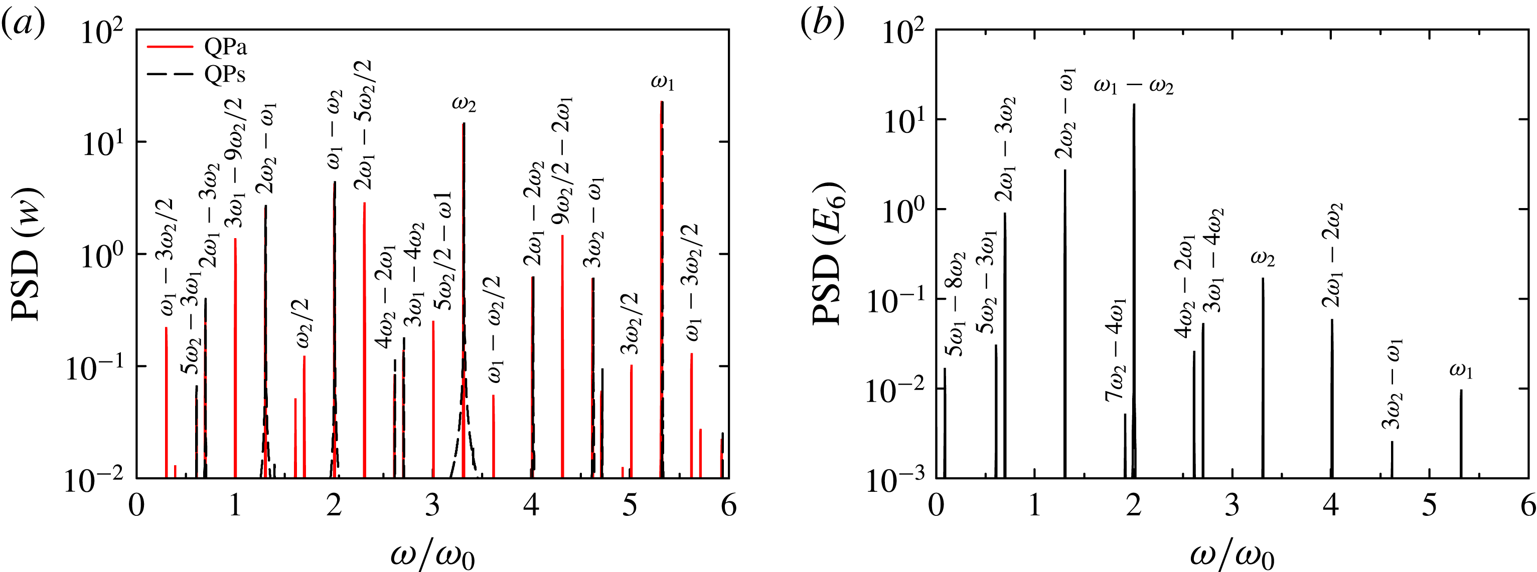
. This indicates that the streaming flow becomes more energetic following the torus-doubling bifurcation. Figure 15(a) shows the PSD of
 $w$
for QPs and QPa at
 ${\it\omega}_{0}=6500$
. The frequencies corresponding to integer combinations of
 ${\it\omega}_{1}$
and
 ${\it\omega}_{2}$
are almost coincidental (differences are less than 0.1 %), but the PSD of QPa also has peaks at
 ${\it\omega}_{2}/2$
and its integer combinations with
 ${\it\omega}_{1}$
, but no peak at
 ${\it\omega}_{1}/2$
. Therefore, the torus doubling corresponds to frequency halving of
 ${\it\omega}_{2}$
, the streaming flow temporal frequency of the QPs/QPa solutions. Figure 15(b) shows the PSD of the modal energy
 $E_{6}$
for QPa at
 ${\it\omega}_{0}=6500$
. The peaks at
 ${\it\omega}_{2}/2$
and its combinations with
 ${\it\omega}_{1}$
are absent, confirming that the two halves of the doubled torus QPa are
 $\mathscr{J}$
-symmetric, so that each half has the same energy and the peak at
 ${\it\omega}_{2}/2$
is not present in the PSD of the modal energies. Moreover, the power of the
 ${\it\omega}_{1}$
peak (the azimuthal rotation frequency of the resonant modes
 $m=5$
and 6) has decreased by three orders of magnitude in comparison with that in figure 15(a). This is consistent with our interpretation that
 ${\it\omega}_{1}$
is essentially an azimuthal rotation frequency (if LC were exactly a rotating wave, the
 ${\it\omega}_{1}$
peak would be absent in the PSD of
 $E_{6}$
).
Variation with
 ${\it\omega}_{0}$
of (a)
 $\mathscr{S}$
and (b) the maxima over long times of the primary modal energies, of the various VLF states for
 ${\it\omega}_{p}/{\it\omega}_{0}=-0.15253$
,
 ${\it\Gamma}=1.62$
and
 ${\it\alpha}=1^{\circ }$
.

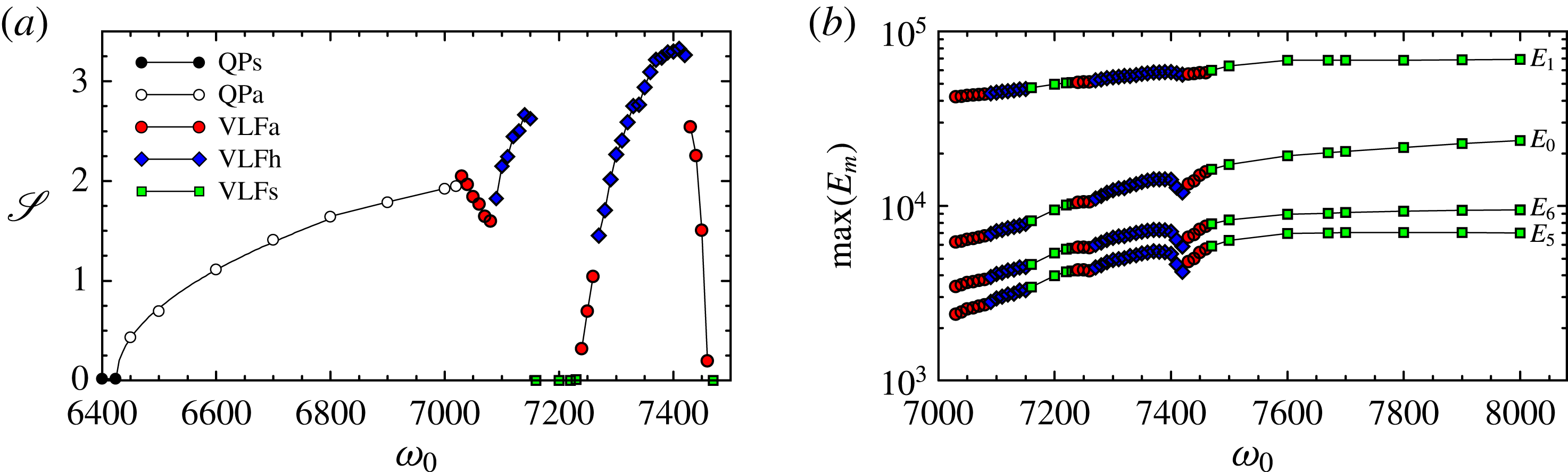
Figure 16(a) shows the variation of
 $\mathscr{S}$
with
 ${\it\omega}_{0}$
for the QPa branch (hollow circles). The symmetry parameter grows as
 $\mathscr{S}\sim ({\it\omega}_{0}-{\it\omega}_{0}^{\mathit{TD}})^{0.5}$
, where
 ${\it\omega}_{0}^{\mathit{TD}}$
is the value of
 ${\it\omega}_{0}$
at the torus-doubling bifurcation, indicating that the bifurcation is supercritical, and that the amplitude behaves as in an ordinary supercritical period-doubling bifurcation. By fitting a square-root profile, the bifurcation value has been estimated to be
 ${\it\omega}_{0}^{\mathit{TD}}\approx 6424$
.
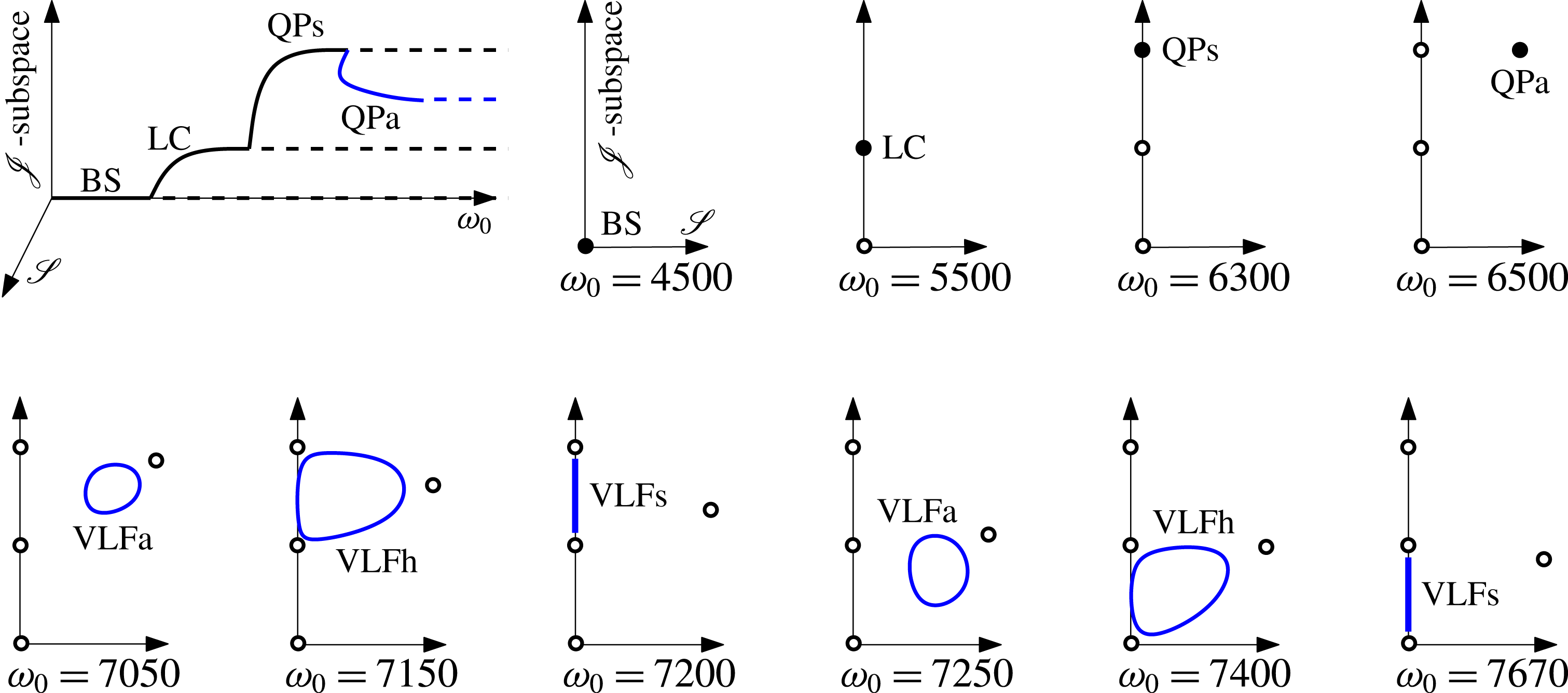
4.4. Very-low-frequency flows and
$\mathscr{J}$
-symmetry restored

On increasing
 ${\it\omega}_{0}$
above 7000, additional bifurcations take place. The new solution branches have an additional very low temporal frequency. Figure 16 shows the variation of
 $\mathscr{S}$
and the maxima over long times of the primary modal energies
 $E_{m}$
of the various VLF states obtained. Figure 17 shows time series of
 $\mathscr{S}$
and the modal energies
 $E_{m}$
, together with the PSD of the VLF state at
 ${\it\omega}_{0}=7050$
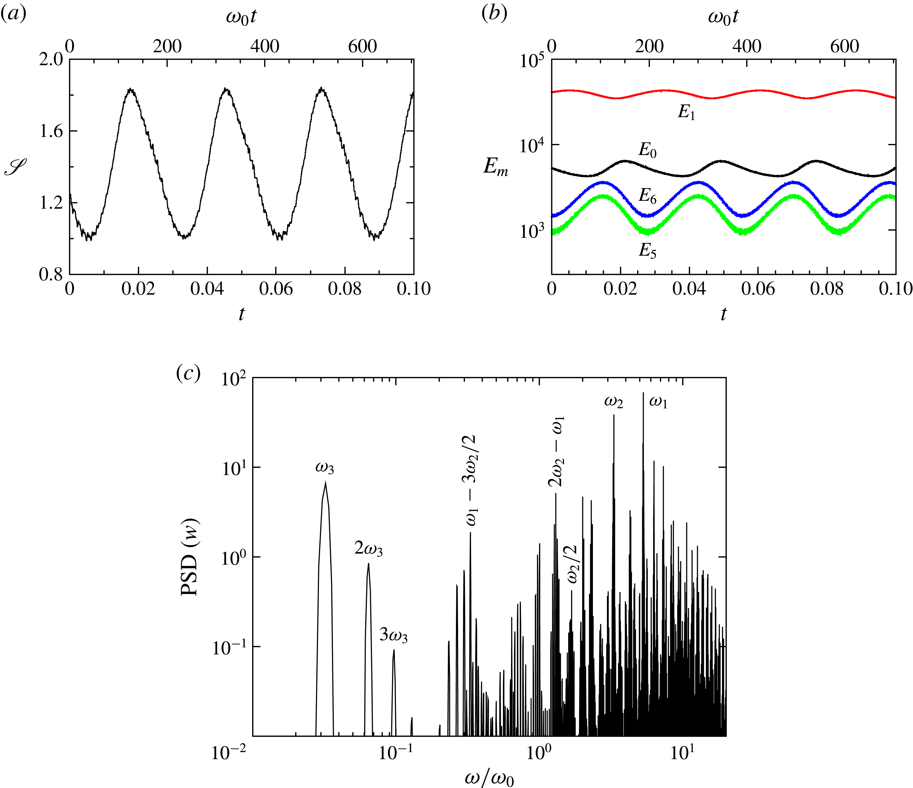
. Since
 $\mathscr{S}\neq 0$
, this VLF state is asymmetric and we have called it VLFa. The time series in figure 17(a,b) show that all variables have a long oscillation period
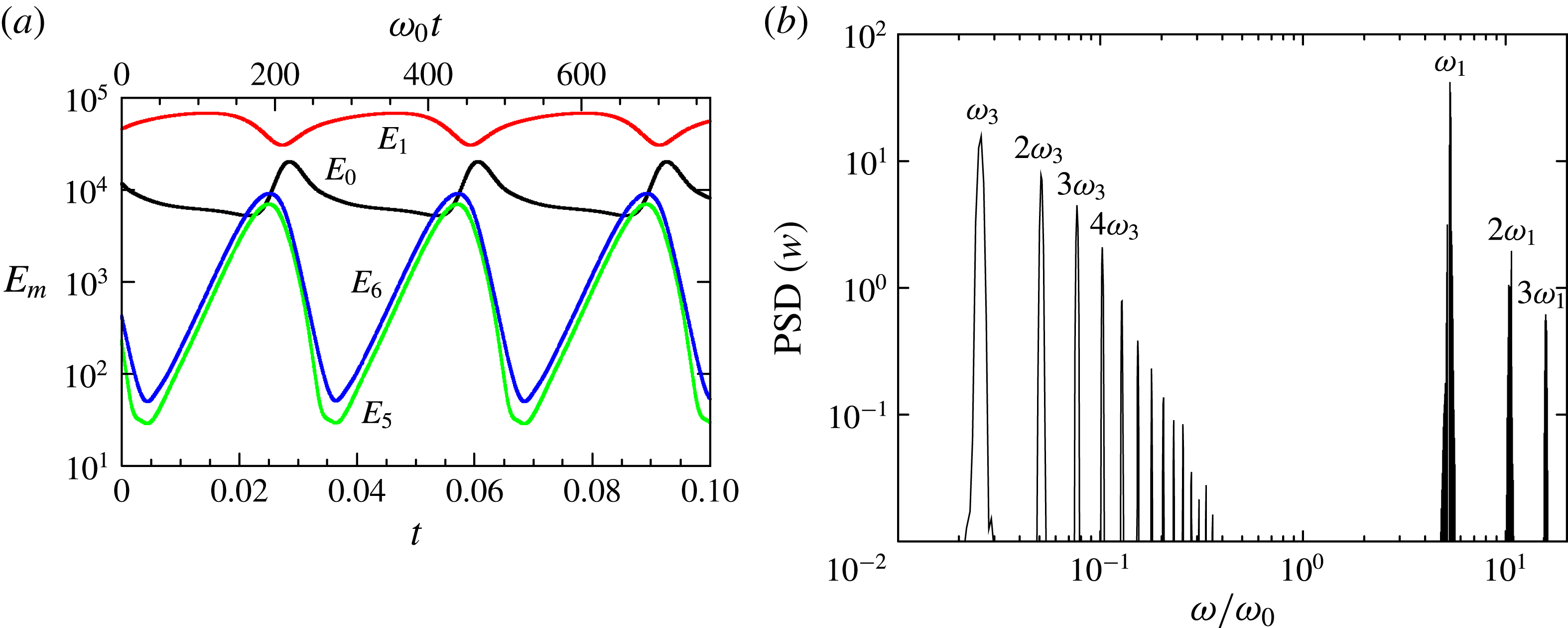
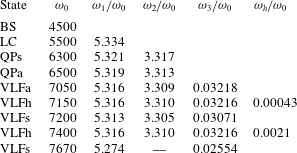
 ${\it\omega}_{0}{\it\tau}_{3}\approx 195$
, corresponding to a very-low-frequency
 ${\it\omega}_{3}/{\it\omega}_{0}\approx 0.0322$
. The frequency
 ${\it\omega}_{3}$
is two orders of magnitude smaller than the azimuthal rotation and streaming frequencies
 ${\it\omega}_{1}$
and
 ${\it\omega}_{2}$
, which are also present in this solution; they can be detected in the power spectral density of this solution shown in figure 17(c) using a log–log plot in order to cover the two orders of magnitude variation between
 ${\it\omega}_{1}$
,
 ${\it\omega}_{2}$
and
 ${\it\omega}_{3}$
. This solution, having three well-defined frequencies, is a three-torus that bifurcates from the QPa state at
 ${\it\omega}_{0}\approx 7025$
. The third frequency
 ${\it\omega}_{3}$
can be interpreted as a periodic approach of the solution to the
 $\mathscr{J}$
-symmetric subspace. This is illustrated in figure 17(a) which shows how
 $\mathscr{S}$
decreases by a factor of approximately two in the time associated with
 ${\it\omega}_{3}$
during its approach towards the
 $\mathscr{J}$
-symmetric subspace and then
 $\mathscr{S}$
grows again as it retreats from the subspace.
For VLFa at
 ${\it\omega}_{0}=7050$
,
 ${\it\omega}_{p}/{\it\omega}_{0}=-0.15253$
,
 ${\it\Gamma}=1.62$
and
 ${\it\alpha}=1^{\circ }$
, (a) shows time series of
 $\mathscr{S}$
, (b) shows time series of
 $E_{0}$
,
 $E_{1}$
,
 $E_{5}$
and
 $E_{6}$
, and (c) shows power spectral density in a
 $\log$
–
 $\log$
plot, showing the very-low-frequency
 ${\it\omega}_{3}$
.

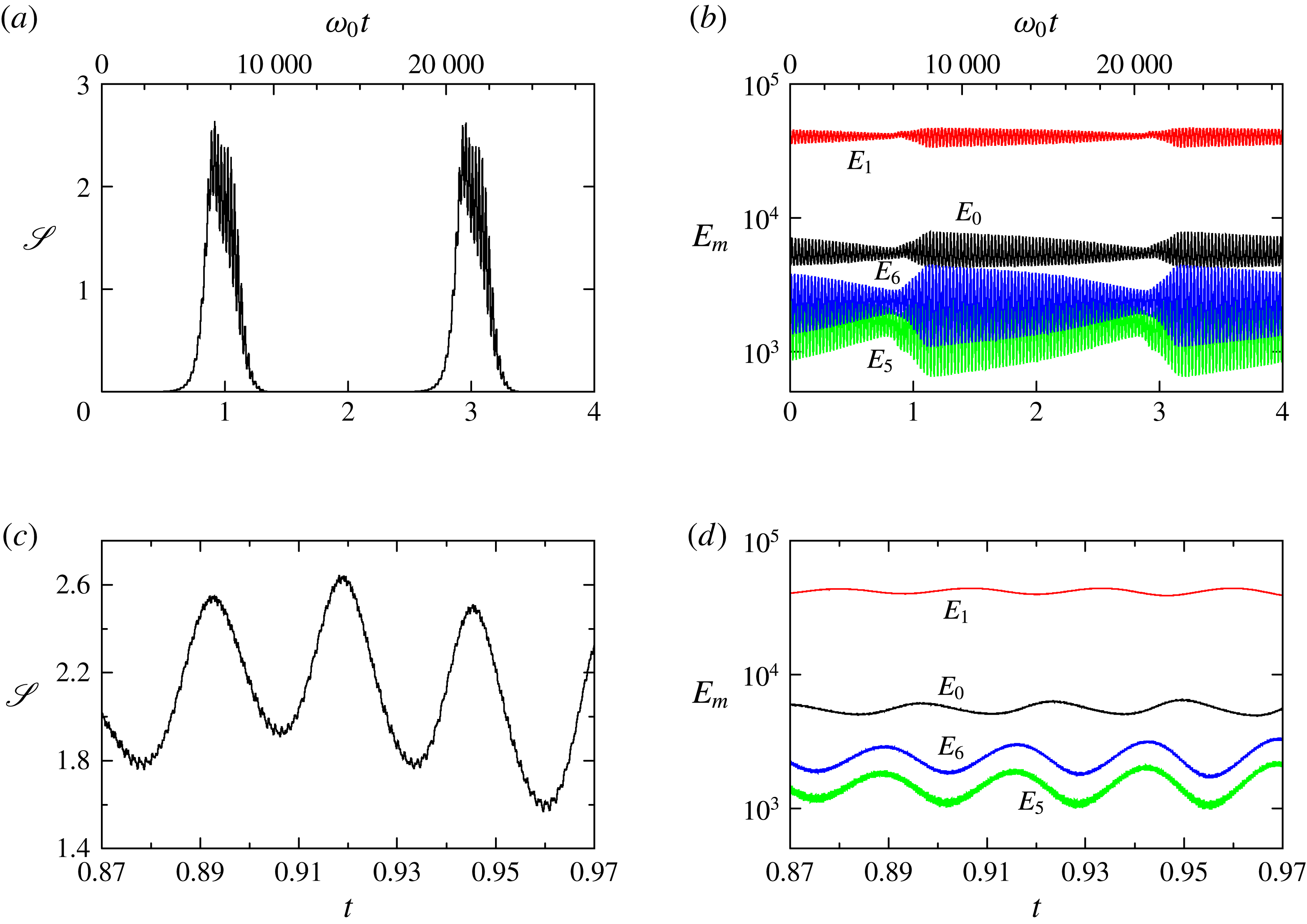
For VLFh at
 ${\it\omega}_{0}=7150$
,
 ${\it\omega}_{p}/{\it\omega}_{0}=-0.15253$
,
 ${\it\Gamma}=1.62$
and
 ${\it\alpha}=1^{\circ }$
, (a) shows time series of
 $\mathscr{S}$
and (b) shows time series of
 $E_{0}$
,
 $E_{1}$
,
 $E_{5}$
and
 $E_{6}$
; (c) and (d) are zooms of (a) and (b) over a time interval that is 40 times smaller.

On increasing
 ${\it\omega}_{0}$
beyond 7085, figure 16(a) shows an abrupt change in the behaviour of
 $\mathscr{S}$
, indicative of another bifurcation. The resulting VLF state, shown in figure 18 at
 ${\it\omega}_{0}=7150$
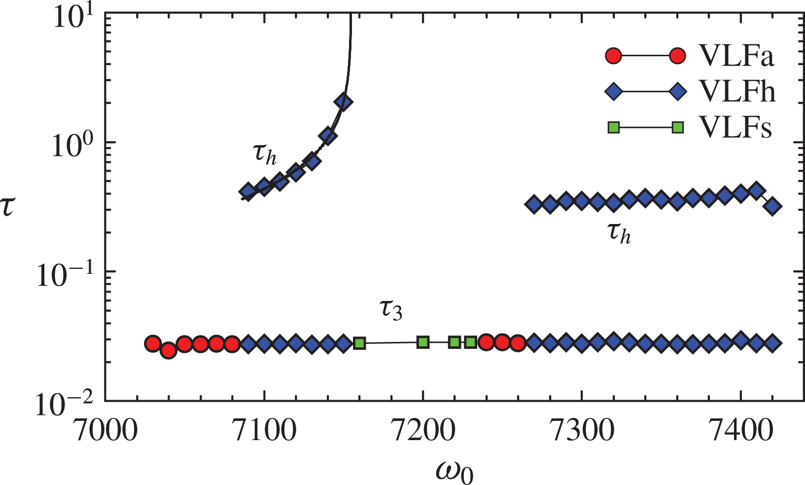
, is very different from VLFa. The period
 ${\it\tau}_{h}$
, corresponding to the variations of
 $\mathscr{S}$
and
 $E_{m}$
shown in figure 18(a,b), is two orders of magnitude larger than
 ${\it\tau}_{3}$
of the previous VLFa branch. This suggests that VLFa (a three-torus) starts to drift with a frequency much smaller than
 ${\it\omega}_{3}$
. For the solution shown in figure 18, this slow drift has a period
 ${\it\tau}_{h}$
of approximately two viscous time units. Figure 18(c,d) shows the same time series as in figure 18(a,b), but over a much smaller time interval. These are very similar to the corresponding time series of VLFa shown in figure 17(a,b), except that they are very slightly modulated by the slow drift. The period
 ${\it\tau}_{h}$
on the new VLF branch goes to infinity at
 ${\it\omega}_{0}\approx 7155$
, a clear signature of homoclinic or heteroclinic dynamics. For this reason we have called this branch VLFh. In figure 18(a),
 $\mathscr{S}$
is almost zero for a long time, a clear indication that this solution spends a long time close to some unstable solution in the
 $\mathscr{J}$
-symmetric subspace. Since
 $E_{5}$
and
 $E_{6}$
are large and oscillating while
 $\mathscr{S}\rightarrow 0$
, this suggests that VLFh approaches QPs for
 $t\gtrsim 1.3$
. Then, later,
 $t\gtrsim 2.5$
, the
 $E_{5}$
and
 $E_{6}$
oscillations decrease, suggesting that the solution approaches closer to LC, before bouncing back (
 $t\gtrsim 3$
) to large values of
 $\mathscr{S}$
, and restarting the heteroclinic cycle again; see figure 18(b).
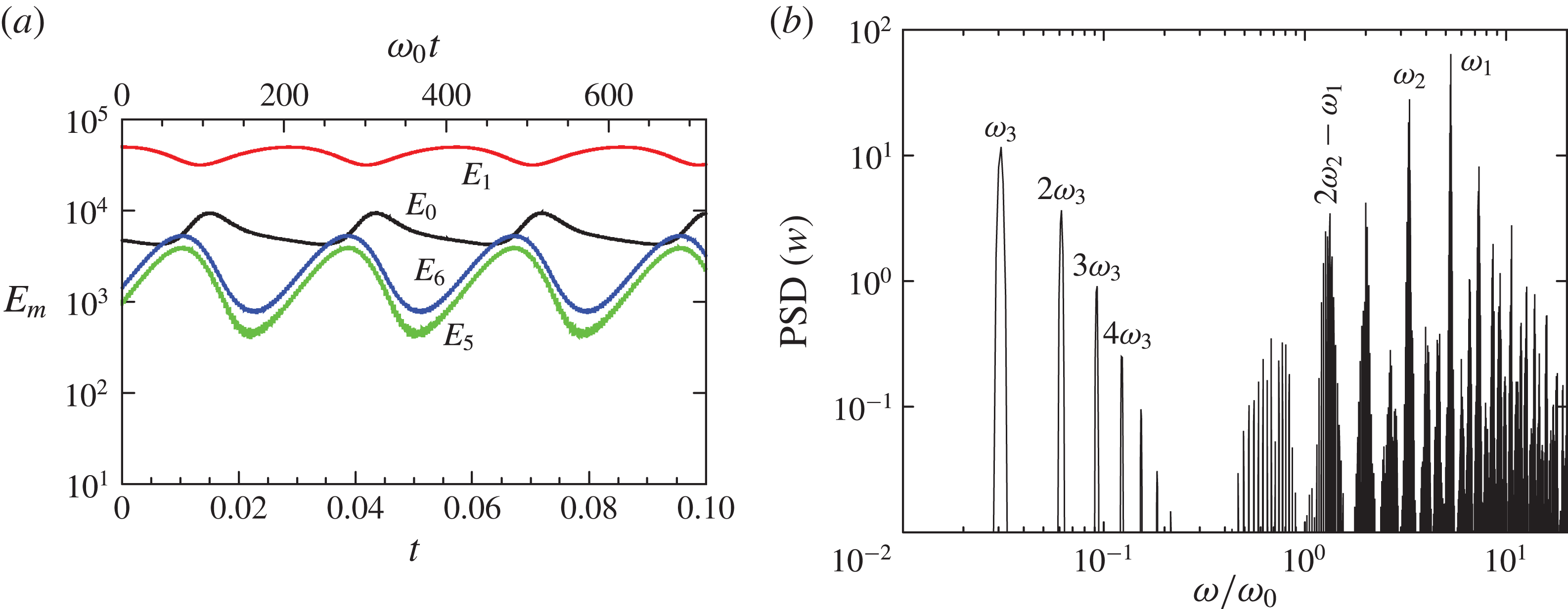
For VLFs at
 ${\it\omega}_{0}=7200$
,
 ${\it\omega}_{p}/{\it\omega}_{0}=-0.15253$
,
 ${\it\Gamma}=1.62$
and
 ${\it\alpha}=1^{\circ }$
, (a) shows time series of the primary modal energies,
 $E_{0}$
,
 $E_{1}$
,
 $E_{5}$
and
 $E_{6}$
, and (b) shows the power spectral density in a
 $\log$
–
 $\log$
plot, showing the very-low-frequency
 ${\it\omega}_{3}$
.

The VLFh branch disappears at the heteroclinic collision, and as can be seen from figure 16(a), the resulting state recovers
 $\mathscr{J}$
-symmetry; we call this branch VLFs. Figure 19 shows time series of the modal energies and the PSD of VLFs at
 ${\it\omega}_{0}=7200$
. The drift has disappeared, and the time series in figure 19(a) are very similar to the corresponding time series of VLFa in figure 17(b). The PSDs of both solutions, VLFs in figure 19(b) and VLFa in figure 17(c), are very similar and the values of
 ${\it\omega}_{1}$
,
 ${\it\omega}_{2}$
and
 ${\it\omega}_{3}$
(relative to
 ${\it\omega}_{0}$
) in the two solutions are almost identical. The only difference between the two PSDs is the absence of the
 ${\it\omega}_{2}/2$
temporal frequency and its combinations with
 ${\it\omega}_{1}$
in the VLFs solution. This is in perfect agreement with the previous observation that
 ${\it\omega}_{2}/2$
appears when the
 $\mathscr{J}$
-symmetry is broken: the asymmetric VLFa has it, but the symmetric VLFs does not. On this VLFs branch,
 ${\it\omega}_{3}$
is not associated with oscillations of the symmetry parameter
 $\mathscr{S}$
, which is zero: the solution is a trajectory inside the
 $\mathscr{J}$
-symmetric subspace. Near the minimum of
 $E_{6}$
in figure 19(a), the relationship between
 $E_{0}$
,
 $E_{5}$
and
 $E_{6}$
is the same as in the QPs state in figure 5(b), where
 $E_{0}$
is larger than
 $E_{5}$
and
 $E_{6}$
. Near the maximum of
 $E_{6}$
in figure 19(a), the relationship between
 $E_{0}$
,
 $E_{5}$
and
 $E_{6}$
is the same as in the LC state in figure 5(b), where
 $E_{0}$
is comparable to
 $E_{5}$
and
 $E_{6}$
. This suggest that VLFs is an oscillation between LC and QPs with frequency
 ${\it\omega}_{3}$
. In fact, both frequencies
 ${\it\omega}_{2}$
and
 ${\it\omega}_{3}$
are present in VLFs (figure 19
b), as well as in QPs (figure 11
b).
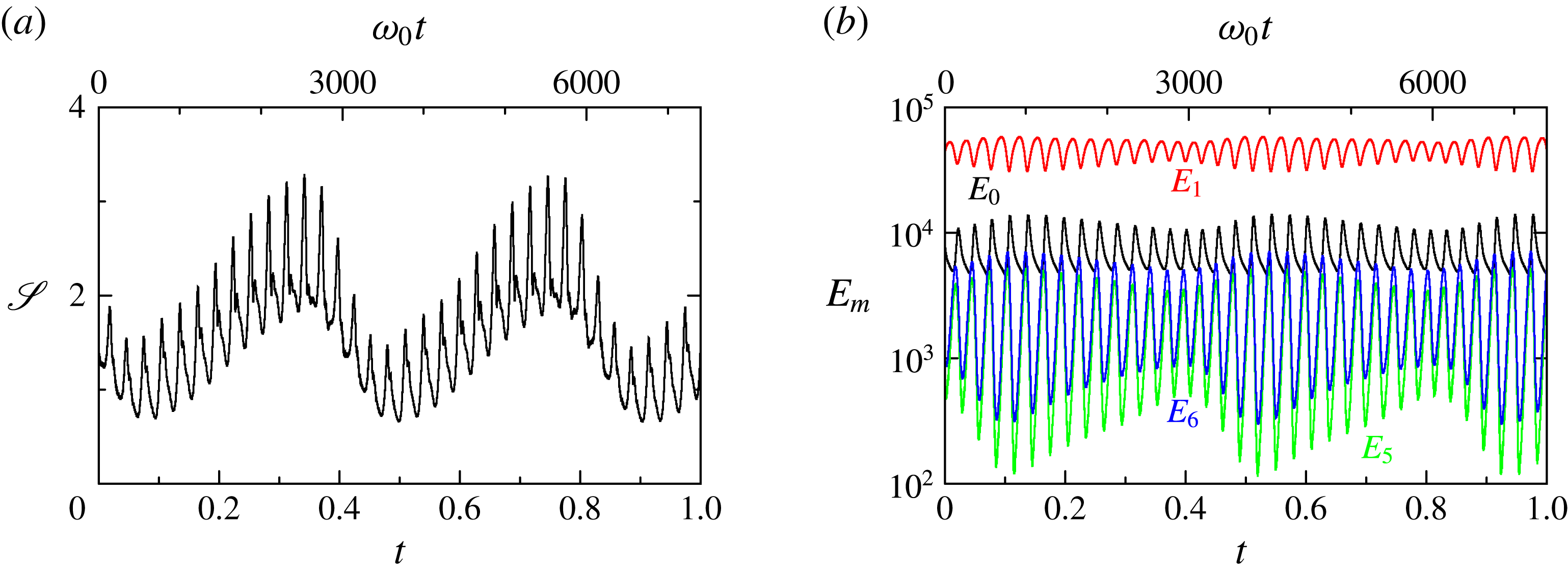
For VLFh at
 ${\it\omega}_{0}=7400$
,
 ${\it\omega}_{p}/{\it\omega}_{0}=-0.15253$
,
 ${\it\Gamma}=1.62$
and
 ${\it\alpha}=1^{\circ }$
, (a) shows time series of
 $\mathscr{S}$
and (b) shows time series of
 $E_{0}$
,
 $E_{1}$
,
 $E_{5}$
and
 $E_{6}$
.

By increasing
 ${\it\omega}_{0}$
beyond 7235, the VLF solutions change again, moving away from the
 $\mathscr{J}$
-symmetric subspace, as shown in figure 16(a). The resulting state is the three-torus solution VLFa described earlier. On increasing
 ${\it\omega}_{0}$
further, at approximately 7265 the VLF solution changes again, becoming the VLFh solution also described earlier. Figure 20 shows time series of
 $\mathscr{S}$
and the primary modal energies of VLFh at
 ${\it\omega}_{0}=7400$
. The period
 ${\it\tau}_{h}$
corresponding to the slow variations of
 $\mathscr{S}$
and
 $E_{m}$
in these plots is 20 times longer than the period
 ${\it\tau}_{3}=2{\rm\pi}/{\it\omega}_{3}$
. Moreover, these time series over a short time span of
 ${\rm\Delta}t=0.1$
show the same behaviour as the other VLFh branch at lower
 ${\it\omega}_{0}$
shown in figure 18(c,d): the solution is almost identical to VLFa on this relatively short time scale. Therefore, this VLFh branch is also a drift of the VLFa solution, with frequency
 ${\it\omega}_{h}=2{\rm\pi}/{\it\tau}_{h}$
. There is an important difference between this VLFh branch and the previous one found in the range
 ${\it\omega}_{0}\in [7085,7155]$
: from the modal energies in figure 20(b), we see that when
 $\mathscr{S}$
approaches its minimum value (at
 $t\sim 0.5$
) the modal energies
 $E_{5}$
and
 $E_{6}$
are one order of magnitude smaller than the corresponding values in the previous branch (figure 18
b). This indicates that the VLFh at
 ${\it\omega}_{0}=7400$
becomes very close to the base state BS, which has almost negligible values of
 $E_{5}$
and
 $E_{6}$
. A detailed analysis of this solution shows that it oscillates between the BS and the LC solutions when it is close to the
 $\mathscr{J}$
-symmetric subspace.
For VLFs at
 ${\it\omega}_{0}=7670$
,
 ${\it\omega}_{p}/{\it\omega}_{0}=-0.15253$
,
 ${\it\Gamma}=1.62$
and
 ${\it\alpha}=1^{\circ }$
, (a) shows time series of
 $E_{0}$
,
 $E_{1}$
,
 $E_{5}$
and
 $E_{6}$
, and (b) shows the power spectral density in a
 $\log$
–
 $\log$
plot.

On increasing
 ${\it\omega}_{0}$
beyond 7425, the VLFh solutions change again, and they evolve into the VLFa branch described earlier. On further increasing
 ${\it\omega}_{0}$
beyond 7465, the VLFa solutions change again, moving into the
 $\mathscr{J}$
-symmetric subspace and resulting in the symmetric state VLFs, as shown in figure 16(a). This new branch of VLFs is stable over a large range of
 ${\it\omega}_{0}$
, extending up to
 ${\it\omega}_{0}=8000$
, as shown in figure 16(b). However, the new VLFs branch is different from the previous VLFs branch that was found for
 ${\it\omega}_{0}\in [7155,7235]$
. Figure 21 shows time series of the modal energies and the PSD of VLFs at
 ${\it\omega}_{0}=7670$
. On comparing the time series of the modal energies in the new branch (figure 21
a) with those of the previous VLFs branch (figure 19
a), we observe that the minimum values of
 $E_{5}$
and
 $E_{6}$
are more than two orders of magnitude smaller than the maximum values, indicating that VLFs drifts very close to the base state BS. On examining this solution at times close to when
 $E_{5}$
and
 $E_{6}$
are largest, we see that it behaves like the limit cycle solution LC. This suggests that the new VLFs branch drifts back and forth between BS and LC inside the
 $\mathscr{J}$
-symmetric subspace. This is confirmed by the PSD of this solution shown in figure 21(b); it clearly shows the presence of the very-low-frequency
 ${\it\omega}_{3}$
, but the streaming frequency
 ${\it\omega}_{2}$
is absent. This is precisely what happens with BS (steady) and LC (with a single frequency
 ${\it\omega}_{1}$
), and therefore
 ${\it\omega}_{3}$
is the frequency of the oscillation of the new VLFs branch drifting between BS and LC.
All of the VLF solutions described share a common feature, associated with the exchange of energy between the resonant modes 5 and 6 (
 $E_{5}$
and
 $E_{6}$
), the streaming flow (
 $E_{0}$
) and the spin-over flow (
 $E_{1}$
). From figures 17(b), 18(d), 19(a) and 21(a), we observe that
 $E_{5}$
and
 $E_{6}$
evolve in phase, showing large oscillations with frequency
 ${\it\omega}_{3}$
. When they start to decrease, the streaming energy
 $E_{0}$
develops a sharp peak, and then remains almost constant until
 $E_{5}$
and
 $E_{6}$
reach their maximum values again. The sharp peak in
 $E_{0}$
coincides with a decrease of
 $E_{1}$
, which recovers again and remains almost constant until the next period
 ${\it\tau}_{3}$
. Therefore,
 ${\it\omega}_{3}$
is associated with the exchange of energy between the resonant
 $m=5$
and
 $m=6$
flow components and the streaming
 $m=0$
flow component. The spin-over
 $m=1$
mode, with a much larger energy than the other modes, acts as a buffer of energy facilitating the exchange between the resonant modes and the streaming flow.
Snapshots of the VLFs state at
 ${\it\omega}_{0}=7670$
,
 ${\it\omega}_{p}=-1170$
,
 ${\it\Gamma}=1.62$
and
 ${\it\alpha}=1^{\circ }$
, showing at five equispaced times over one period
 ${\it\tau}_{3}\approx 0.032$
contours of the axial vorticity at (a)
 $z=-0.25{\it\Gamma}$
and (b)
 $z=0$
, (c) the axial velocity at
 $z=0$
and (d) the helicity at
 $z=0$
. See online movies.

Contours of the
 $m=0$
azimuthal Fourier component of the azimuthal velocity,
 $v_{0}$
(deviation with respect to solid-body rotation), of the VLFs state at
 ${\it\omega}_{0}=7670$
,
 ${\it\omega}_{p}=-1170$
,
 ${\it\Gamma}=1.62$
and
 ${\it\alpha}=1^{\circ }$
at five equispaced times over one period
 ${\it\tau}_{\mathit{VLFs}}\approx 0.032$
: (a)
 $t=t_{1}=0.0064$
, (b)
 $t=2t_{1}$
, (c)
 $t=3t_{1}$
, (d)
 $t=4t_{1}$
, (e)
 $t=5t_{1}$
. See online movie.

Isosurfaces of the axial velocity (a–e) and helicity (f–j), at levels
 $w=50$
and
 $\mathscr{H}=\pm 10^{6}$
, of the VLFs state at
 ${\it\omega}_{0}=7670$
,
 ${\it\omega}_{p}=-1170$
,
 ${\it\Gamma}=1.62$
and
 ${\it\alpha}=1^{\circ }$
at five equispaced times over one period
 ${\it\tau}_{\mathit{VLFs}}\approx 0.032$
: (a,f)
 $t=t_{1}=0.0064$
, (b,g)
 $t=2t_{1}$
, (c,h)
 $t=3t_{1}$
, (d,i)
 $t=4t_{1}$
, (e,j)
 $t=5t_{1}$
. See online movies.

The VLFs at
 ${\it\omega}_{0}=7670$
,
 ${\it\omega}_{p}=-1170$
,
 ${\it\Gamma}=1.62$
and
 ${\it\alpha}=1^{\circ }$
has been studied in detail in the experiments of Lagrange et al. (Reference Lagrange, Eloy, Nadal and Meunier2008), and in Lagrange et al. (Reference Lagrange, Meunier, Nadal and Eloy2011) a weakly nonlinear model was developed which captures many features of the flow. Figure 22 shows snapshots at a few different times during the very-low-frequency oscillation (whose period is
 ${\it\tau}_{3}\approx 0.032$
) of various quantities. Here, (a) shows the axial vorticity at
 $z=-0.25{\it\Gamma}$
; this is the same quantity at the same axial location that corresponds to the experimental particle image velocimetry measurements in Lagrange et al. (Reference Lagrange, Eloy, Nadal and Meunier2008, Reference Lagrange, Meunier, Nadal and Eloy2011). The first snapshot is at a time when
 $E_{5}$
and
 $E_{6}$
are close to their minimum values (see the modal energy time series for this solution in figure 21), and the flow looks very much like the basic state (compare with BS at
 ${\it\omega}_{0}=4500$
shown in figure 4). One interesting difference is the orientation of the axial velocity at mid-height; for BS the zero-
 $w$
contour is almost horizontal, whereas for VLFs it is distinctly inclined. This is probably due to the much stronger streaming flow at the larger
 ${\it\omega}_{0}$
;
 $E_{1}/E_{0}$
is of order 20 for BS and of order 4 for VLFs. The spatial structure of the streaming flow,
 $v_{0}$
, for this VLFs state is shown in figure 23 at the same times. The structure of
 $v_{0}$
of VLFs at the first snapshot is very much like that of BS shown in figure 4(d). By the fourth snapshot,
 $E_{5}$
and
 $E_{6}$
are at their maxima, and as noted by Lagrange et al. (Reference Lagrange, Meunier, Nadal and Eloy2011), the nonlinear interactions of these eigenmodes among themselves and with the viscous boundary layers lead to enhanced axisymmetric streaming flow. The time series (figure 21) shows that as
 $E_{5}$
and
 $E_{6}$
reach their maxima,
 $E_{0}$
suddenly spikes up. It does so in a very localized fashion; figure 23(d) shows that this spike corresponds to a region at approximately 80 % radius, where the vertical velocity and helicity associated with the
 $m=5$
and
 $m=6$
components of the flow are strongest. In this region, the streaming flow develops a strong shear between the core region, which precesses counterclockwise, and the region close to the cylinder wall, which precesses clockwise. This complex interaction with the streaming flow has the tendency to bring the zero-
 $w$
contour line at mid-height back towards horizontal. During this phase of the slow oscillation, the VLF state closely resembles the LC state. The three-dimensional isosurfaces of axial velocity and helicity shown in figure 24 further illustrate this. The isosurfaces at
 $t=0.0064$
in figure 24 should be compared with those corresponding to BS in figure 3(a,e), and those at
 $t=0.0256$
should be compared with those corresponding to LC in figure 10. All of the broad aspects of the VLFs are well described from the experimental observations detailed in Lagrange et al. (Reference Lagrange, Meunier, Nadal and Eloy2011); their weakly nonlinear model captures many of those aspects. It seems that perhaps where their model is lacking is that it does not include the
 $v_{0}$
streaming flow contribution from the forced
 $m=1$
component of the flow. Of course, it is difficult to account for the viscous nonlinear interaction terms in any precise way without solving the complete problem, as we have done numerically.
Frequencies of the solutions obtained inside the resonance horn (
 ${\it\omega}_{p}/{\it\omega}_{0}=-0.15253$
,
 ${\it\Gamma}=1.62$
and
 ${\it\alpha}=1^{\circ }$
), scaled with the solid-body rotation frequency
 ${\it\omega}_{0}$
.

Variations with
 ${\it\omega}_{0}$
of
 ${\it\tau}_{3}$
of VLFa, VLFs and VLFh, and of
 ${\it\tau}_{h}$
of VLFh for
 ${\it\omega}_{p}/{\it\omega}_{0}=-0.15253$
,
 ${\it\Gamma}=1.62$
and
 ${\it\alpha}=1^{\circ }$
.

Table 1 shows the values of the four frequencies
 ${\it\omega}_{1}$
,
 ${\it\omega}_{2}$
,
 ${\it\omega}_{3}$
and
 ${\it\omega}_{h}$
for the solutions we have so far analysed in detail (increasing
 ${\it\omega}_{0}$
above 8000 results in more complicated states whose analysis is beyond the scope of the present study). On scaling these frequencies with the solid-body rotation frequency
 ${\it\omega}_{0}$
, we observe that
 ${\it\omega}_{1}$
and
 ${\it\omega}_{2}$
are almost constant over the entire
 ${\it\omega}_{0}$
range, with variations smaller than 1 %;
 ${\it\omega}_{3}$
is also almost constant for VLF solutions outside the
 $\mathscr{J}$
-symmetric subspace, and has larger variations (up to 20 %) for VLF solutions in the
 $\mathscr{J}$
-symmetric subspace.
The behaviour of
 ${\it\omega}_{h}$
with
 ${\it\omega}_{0}$
is more complicated, and shows very large variations associated with the fact that heteroclinic collisions appear, and in them
 ${\it\omega}_{h}$
goes to zero and the corresponding period
 ${\it\tau}_{h}$
goes to infinity. The variation of
 ${\it\tau}_{h}$
with
 ${\it\omega}_{0}$
along the two branches of VLFh is shown in figure 25. We have also included the period
 ${\it\tau}_{3}$
corresponding to
 ${\it\omega}_{3}$
of various VLF states for comparison. We observe that
 ${\it\tau}_{h}\rightarrow \infty$
in the first VLFh branch that terminates in a heteroclinic collision; a convenient fit has been added to guide the eye. In contrast, in the second VLFh branch,
 ${\it\tau}_{h}$
is almost constant, and one order of magnitude larger than
 ${\it\tau}_{3}$
. We have not explored in minute detail the dynamics of the VLF branches because of the extremely large computational time required to compute the long periods associated with
 ${\it\omega}_{3}$
and
 ${\it\omega}_{h}$
, and also because the transients following changes to
 ${\it\omega}_{0}$
are extremely long. It is possible that these VLF branches coexist in some parameter ranges, and the transitions between them present hysteresis. It is also possible that other heteroclinic collisions take place, in very small parameter ranges.
5. Traverse in precession rate
${\it\omega}_{p}$
, keeping the cylinder rotation
${\it\omega}_{0}=7670$


So far, all of the results we have presented have been nominally in the resonance corresponding to
 ${\it\omega}_{p}/{\it\omega}_{0}=-0.15253$
, and we considered the dynamics as the effects of viscosity were reduced (by increasing
 ${\it\omega}_{0}$
). Generally, viscosity tends to broaden the region of resonance and perhaps introduce detuning effects. In this section, we explore what happens as the resonance is traversed, keeping
 ${\it\omega}_{0}=7670$
,
 ${\it\Gamma}=1.62$
and
 ${\it\alpha}=1^{\circ }$
while varying
 ${\it\omega}_{p}$
, i.e. traversing the resonance through the VLFs state shown in figure 22. The range of
 ${\it\omega}_{p}$
considered is
 ${\it\omega}_{p}\in [-1000,-1400]$
, which in terms of the forcing frequency used by Lagrange et al. (Reference Lagrange, Eloy, Nadal and Meunier2008, Reference Lagrange, Meunier, Nadal and Eloy2011) corresponds to
 ${\it\omega}_{f}\in [1.15,1.22]$
, with the theoretical resonance frequency being
 ${\it\omega}_{f}=1.18$
(
 ${\it\omega}_{p}/{\it\omega}_{0}=-0.15253$
).
Variations of the primary modal energies with
 ${\it\omega}_{p}$
while keeping
 ${\it\omega}_{0}=7670$
;
 ${\it\omega}_{p}\in [-1400,-1000]$
corresponds to
 ${\it\omega}_{f}\in [1.22,1.15]$
.

Figure 26, which shows the relevant modal energies of the different solutions found traversing the resonance, summarizes our results. When moving into the resonance from afar, starting from the base state, we find a succession of bifurcations through states that we have already described, with increasing complexity: the LC, the quasiperiodic solutions and finally the very-low-frequency solutions. The peak of the resonance is dominated by the two-torus VLFs solution described in figures 22 and 23, due to our choice of
 ${\it\omega}_{0}=7670$
. The most noticeable feature in figure 26 is that the resonance is not symmetric. Upon entering the resonance peak from small values of
 $|{\it\omega}_{p}|$
, we observe that the
 $\mathscr{J}$
-symmetric solutions QPs are absent, and a rapid succession of bifurcations in a small parameter range takes place, involving several VLF states, mainly asymmetric, and with clear indications of hysteretic behaviour. Then, just before reaching the resonance peak, the
 $\mathscr{J}$
-symmetry is restored, and the two-torus VLFs solution emerges. On exiting the resonance peak by increasing
 $|{\it\omega}_{p}|$
, the situation is much simpler. All of the solutions obtained are
 $\mathscr{J}$
-symmetric, and the three-torus solutions are absent. From the two-torus VLFs with frequencies
 ${\it\omega}_{1}$
and
 ${\it\omega}_{3}$
we jump to the QPs solution branch with frequencies
 ${\it\omega}_{1}$
and
 ${\it\omega}_{2}$
, and this branch bifurcates back to the limit cycle LC with the single frequency
 ${\it\omega}_{1}$
, and then to the base state steady solution.
6. Discussion and conclusions
We have studied in detail the nonlinear dynamics of the precession flow in a small parameter neighbourhood where the forced spin-over flow is predicted to be resonant in the linearized inviscid theory with two additional Kelvin modes that form a resonant triad with the forced mode. In any physical experiment, the secular unbounded resonant growth is halted by various processes, such as viscous damping and nonlinear saturation. Lagrange et al. (Reference Lagrange, Meunier, Nadal and Eloy2011) determined the parameter regime where this is expected using the linear inviscid theory, conducted experiments showing the triadic resonance, and further developed a weakly nonlinear theory that captures many aspects of what is observed experimentally. For the weakly nonlinear theory to produce dynamics that are close to the experimental observations, an estimate of the strength of the axisymmetric streaming flow that results from nonlinear viscous interactions needed to be incorporated using data from the experimental observations. They only included such contributions from the flow components that are excited via the triadic resonance, and neglected contributions from the primary forced flow. Nevertheless, the theory gives very good estimates of the parameter values at which the triadic resonance occurs, and of the time scales of some of the flows that result. The details of the bifurcations involved could not be resolved experimentally as they required variations in the governing parameters much finer than were experimentally accessible, and the weakly nonlinear theory on its own was inadequate as it required input from the experiments to adjust the fitting parameter characterizing the streaming flow. It is precisely in this parameter regime where we have conducted our study, clarifying in detail the nonlinear dynamics involved, via direct numerical simulations of the Navier–Stokes equations and the use of dynamical systems theory with symmetries.
Recently, Albrecht et al. (Reference Albrecht, Blackburn, Lopez, Manasseh and Meunier2015) have considered the robustness of the triadic-resonance mechanism using direct numerical simulations by including cases where detuning effects are present. For finely tuned cylinders, experiments and weakly nonlinear theory (Lagrange et al. Reference Lagrange, Eloy, Nadal and Meunier2008, Reference Lagrange, Meunier, Nadal and Eloy2011) had already shown that triadic resonance is at play, and here we have investigated in detail the bifurcations involved. The numerical technique used in Albrecht et al. (Reference Albrecht, Blackburn, Lopez, Manasseh and Meunier2015), the spectral element method, is quite different from the spectral collocation method used here. For the cases computed in common, excellent agreement is achieved, providing confidence in both numerical techniques, beyond that afforded by comparisons with experimental data.
The triadic resonance investigated takes place for a cylinder of aspect ratio
 ${\it\Gamma}=1.62$
that has forced frequency
 ${\it\omega}_{f}=1.18$
, corresponding to a Poincaré number
 ${\it\omega}_{p}/{\it\omega}_{0}=-0.15253$
. By keeping these parameters fixed, as well as fixing the tilt angle to
 ${\it\alpha}=1^{\circ }$
while increasing
 ${\it\omega}_{0}$
(reducing the influence of viscosity in the system), we have found that the base state, corresponding to the forced spin-over flow with azimuthal wavenumber
 $m=1$
, is stable up to
 ${\it\omega}_{0}\approx 4777$
. For smaller
 ${\it\omega}_{0}$
viscous effects dominate the flow. This is consistent with experimental observations of Lagrange et al. (Reference Lagrange, Eloy, Nadal and Meunier2008, Reference Lagrange, Meunier, Nadal and Eloy2011), as well as with their weakly nonlinear theory when detuning and volume viscous effects are included (if detuning and volume viscous effects are not included, their theory predicts a critical
 ${\it\omega}_{0}$
that is considerably smaller). Above the critical
 ${\it\omega}_{0}$
value, the triadic resonance comes into play. In the first bifurcation, the resonant modes with azimuthal wavenumbers
 $m=5$
and
 $m=6$
bifurcate from the base state, both with the same frequency
 ${\it\omega}_{1}$
, in agreement with the triadic-resonance theory. The result is a limit cycle LC whose
 $m=5$
and
 $m=6$
azimuthal components rotate in the azimuthal direction almost uniformly.
We have made detailed comparisons of the LC state with the theory of triadic resonant Kelvin modes (the theory is summarized in appendix B): not only is the triadic resonance manifested at the specified values of
 ${\it\Gamma}$
and
 ${\it\omega}_{p}$
, but the frequency of LC coincides with the frequency of the resonant
 $m=5$
and 6 Kelvin modes, with the difference between the frequencies from the nonlinear LC state and the linear theory being less than 0.5 %. The structure of the
 $m=5$
and 6 Kelvin modes is clearly apparent in the LC state, but there are also significant differences due to the nonlinearities and the presence of strong viscous boundary layers. There are two main differences. One is that LC has a strong
 $m=0$
streaming flow, which is not geostrophic, due to the presence of inertial-wave beams originating from the boundary layers. The other difference is the complex structure of the helicity of LC, due mainly to the nonlinear interactions between the different components of the flow. We have also compared the critical value of
 ${\it\omega}_{0}$
, where LC bifurcates from BS, with the corresponding value from the reduced model of Lagrange et al. (Reference Lagrange, Meunier, Nadal and Eloy2011), and both results agree to within 4 %.
On increasing
 ${\it\omega}_{0}$
, LC loses stability at a secondary Hopf bifurcation to a two-torus state QPs. The new frequency introduced at the bifurcation,
 ${\it\omega}_{2}$
, is smaller than but close to
 ${\it\omega}_{1}$
and corresponds to a radial oscillation of the streaming flow, which becomes time-dependent. This oscillation is also associated with modifications in the
 $m=5$
and
 $m=6$
flow components. These components of the flow also introduce wave beams into the bulk, and as the various components active in the triadic resonance and their impacts on the boundary layers are less damped by viscosity with increasing
 ${\it\omega}_{0}$
, the flow becomes more spatio-temporally complex. The governing equations are invariant under a spatial symmetry, the inversion
 $\mathscr{J}$
, and the states described so far (BC, LC and QPs) are also
 $\mathscr{J}$
-invariant. This symmetry is broken in the following bifurcation of QPs, resulting in an asymmetric two-torus QPa. This sequence of bifurcations resembles the classical Ruelle–Takens route to chaos (Ruelle & Takens Reference Ruelle and Takens1971; Newhouse, Ruelle & Takens Reference Newhouse, Ruelle and Takens1978), and is illustrated at the top of figure 27, showing a schematic bifurcation diagram and selected schematic phase portraits of the solutions analysed in detail in this study.
Schematic bifurcation diagram and selected phase portraits of the different solutions obtained. The states BS, LC and QPs are all in the
 $\mathscr{J}$
-symmetric subspace (
 $\mathscr{S}=0$
), while QPa and most of the VLF states are not (
 $\mathscr{S}\neq 0$
). Stable states are shown as solid disks and thick lines, while unstable states are hollow disks.

According to the Ruelle–Takens scenario, the next bifurcation would result in chaotic dynamics. What we obtain in this problem is different. At
 ${\it\omega}_{0}\approx 7025$
the two-torus QPa state bifurcates to a three-torus state with an additional very-low-frequency
 ${\it\omega}_{3}$
. In the range
 ${\it\omega}_{0}\in [7025,8000]$
, a variety of VLF states are found, and schematic phase portraits of these are shown at the bottom of figure 27. The third frequency
 ${\it\omega}_{3}$
is associated with the exchange of energy between the resonant
 $m=5$
and
 $m=6$
flow components and the
 $m=0$
streaming flow component, and corresponds to an oscillation between some of the four states obtained in the first three bifurcations (BS, LC, QPs and QPa), which are now all unstable. In addition, we have also obtained branches of solutions corresponding to slow drifts of the three-torus states. These wander in phase space between some of the unstable states, and for some
 ${\it\omega}_{0}$
values they become heteroclinic to some of them. Moreover, some of these states also move in and out of the
 $\mathscr{J}$
-symmetric subspace, as illustrated at the bottom of figure 27. These VLF states are quasiperiodic three-torus or weakly chaotic states, and the heteroclinic dynamics found suggests the presence of chaotic attractors in the neighbourhood of these heteroclinic collisions.
We have also analysed the bifurcations that take place when traversing the resonance at a fixed
 ${\it\omega}_{0}=7670$
, while varying
 ${\it\omega}_{p}$
. We have found that the resonance peak is asymmetric, with the side corresponding to small values of
 $|{\it\omega}_{p}|$
dominated by asymmetric states involved in a complex sequence of bifurcations over a narrow parameter range, involving three-torus solutions and hysteresis. In contrast, the side corresponding to larger values of
 $|{\it\omega}_{p}|$
is much simpler, consisting of
 $\mathscr{J}$
-symmetric states that are at most two-torus, and no hysteresis has been observed. This asymmetry of the resonant peak is typical of nonlinear oscillators: the resonance peak is tilted to one side, resulting in hysteretic jumps appearing only on the tilted side (Jordan & Smith Reference Jordan and Smith2007). The very-low-frequency
 ${\it\omega}_{3}$
is present on both sides of the resonance; however, states with both
 ${\it\omega}_{3}$
and
 ${\it\omega}_{2}$
, the frequency associated with the temporal oscillation of the streaming flow, appear only on the side with small values of
 $|{\it\omega}_{p}|$
, where complex dynamics of three-torus is present.
The slow drifts between various unstable states, characteristic of the VLF solutions, occur on a viscous time scale. In typical experiments (Manasseh Reference Manasseh1992, Reference Manasseh1994; Lagrange et al.
Reference Lagrange, Eloy, Nadal and Meunier2008, Reference Lagrange, Meunier, Nadal and Eloy2011; Meunier et al.
Reference Meunier, Eloy, Lagrange and Nadal2008) the cylinder radius is between 2 and 10 cm, and the working fluid is water with a nominal kinematic viscosity of approximately
 $0.01~\text{cm}^{2}~\text{s}^{-1}$
, giving viscous times of between 200 s and 2.8 h. Given that the bifurcations we have described are separated by variations in the governing parameters of less than 0.5 %, maintaining the flow conditions over several viscous times constant to within a tolerance of order 0.1 % can present a major challenge, particularly for the larger cylinders, while continuously acquiring data during that time in order to resolve the slow-drift dynamics. Nevertheless, some of the slow-drift dynamics, such as the VLFs state at
 ${\it\omega}_{0}=7670$
,
 ${\it\omega}_{p}=-1170$
,
 ${\it\Gamma}=1.62$
, and
 ${\it\alpha}=1^{\circ }$
, have been clearly captured experimentally and largely explained in terms of a weakly nonlinear theory (Lagrange et al.
Reference Lagrange, Eloy, Nadal and Meunier2008, Reference Lagrange, Meunier, Nadal and Eloy2011), and with the numerical simulations of the full problem, we now have a much clearer understanding of this state being a slow drift between unstable states in the system.
It is worth mentioning that this VLFs state at large
 ${\it\omega}_{0}$
is stable over a large parameter range (see figure 16
b), and has a simple temporal behaviour (it is a two-torus, with two well-defined frequencies
 ${\it\omega}_{1}$
and
 ${\it\omega}_{3}$
), in contrast with the other VLF states, which are three-torus, exist in small parameter ranges and exhibit complicated bifurcations, including homoclinic and heteroclinic dynamics. It is this complicated dynamics that we have elucidated in the present study, which had not been previously analysed experimentally, theoretically or numerically.
So far, all of the states found in this study have either been point-wise
 $\mathscr{J}$
-symmetric (where the state at any point in time is
 $\mathscr{J}$
-invariant), or set-wise
 $\mathscr{J}$
-symmetric (where the state at any point in time is not
 $\mathscr{J}$
-invariant, but evolved in a space that is
 $\mathscr{J}$
-invariant). Such states, even if they have complicated spatio-temporal dynamics, are not turbulent in the sense that because of their symmetry they have long-range correlations in both space and time. It is evident that a transition to turbulence in the precessing flow will have to involve the complete destruction of the
 $\mathscr{J}$
-symmetry.
Acknowledgements
This work was supported by the National Science Foundation grant CBET-1336410 and the Spanish Ministry of Education and Science/FEDER grant FIS2013-40880-P.
Supplementary movies
Supplementary movies are available at http://dx.doi.org/10.1017/jfm.2015.524.
Appendix A. Background on PDEs with symmetry
A symmetry operation
 $\unicode[STIX]{x1D64E}$
acting on Cartesian coordinates as an orthogonal matrix (
 $\boldsymbol{x}\mapsto \unicode[STIX]{x1D64E}\boldsymbol{x}$
) can be extended in a natural way to scalar and vector fields. The natural action
 $\mathscr{A}(\unicode[STIX]{x1D64E})$
on scalar functions
 $f(\boldsymbol{x})$
, such as pressure or temperature, and vectors
 $\boldsymbol{v}(\boldsymbol{r})$
, such as the velocity field, is given by Chossat & Lauterbach (Reference Chossat and Lauterbach2000):
 $$\begin{eqnarray}\mathscr{A}(\unicode[STIX]{x1D64E})f(\boldsymbol{x})=f(\unicode[STIX]{x1D64E}^{-1}\boldsymbol{x}),\quad \mathscr{A}(\unicode[STIX]{x1D64E})\boldsymbol{v}(\boldsymbol{x})=\unicode[STIX]{x1D64E}\boldsymbol{v}(\unicode[STIX]{x1D64E}^{-1}\boldsymbol{x}).\end{eqnarray}$$
These new fields
 $\mathscr{A}(\unicode[STIX]{x1D64E})f$
and
 $\mathscr{A}(\unicode[STIX]{x1D64E})\boldsymbol{v}$
are called the
 $\unicode[STIX]{x1D64E}$
-transformed fields; they are also referred to as the fields that are symmetry related by
 $\unicode[STIX]{x1D64E}$
to the original fields. The natural action in (A 1) is appropriate for the velocity field and in general for the so-called polar vector fields. The natural action for an axial vector field
 ${\bf\omega}$
(such as the vorticity or the vector product of polar fields) is slightly different:
 $$\begin{eqnarray}\mathscr{A}(\unicode[STIX]{x1D64E}){\bf\omega}(\boldsymbol{x})=(\det \unicode[STIX]{x1D64E})\unicode[STIX]{x1D64E}{\bf\omega}(\unicode[STIX]{x1D64E}^{-1}\boldsymbol{x}).\end{eqnarray}$$
It should be noted that for orthogonal matrices,
 $\unicode[STIX]{x1D64E}^{-1}=\unicode[STIX]{x1D64E}^{\text{T}}$
and
 $\det \unicode[STIX]{x1D64E}=\pm 1$
.
A vector field
 $\boldsymbol{u}$
(polar or axial) is
 $\unicode[STIX]{x1D64E}$
-symmetric, or equivariant under
 $\unicode[STIX]{x1D64E}$
, if
 $\mathscr{A}(\unicode[STIX]{x1D64E})\boldsymbol{u}(\boldsymbol{r})=\boldsymbol{u}(\boldsymbol{r})$
, i.e. if it coincides with the
 $\unicode[STIX]{x1D64E}$
-transformed field; an equivalent expression is
 $\unicode[STIX]{x1D64E}\boldsymbol{v}(\boldsymbol{r})=\boldsymbol{v}(\unicode[STIX]{x1D64E}\boldsymbol{r})$
for polar fields and
 $\unicode[STIX]{x1D64E}{\bf\omega}(\boldsymbol{r})=(\det \unicode[STIX]{x1D64E}){\bf\omega}(\unicode[STIX]{x1D64E}\boldsymbol{r})$
for axial fields.
The Navier–Stokes equations are PDEs that depend on the velocity field
 $\boldsymbol{v}$
and the pressure field
 $p$
. We indicate this dependence as
 $\boldsymbol{N}[\boldsymbol{v},p]$
. Here,
 $\boldsymbol{N}$
is a vector field that depends on other scalar and vector fields, and in general the dependence will be nonlinear and involve space and time derivatives. We say that the PDE
 $\boldsymbol{N}=0$
is equivariant under
 $\unicode[STIX]{x1D64E}$
if
 $$\begin{eqnarray}\mathscr{A}(\unicode[STIX]{x1D64E})\boldsymbol{N}[\boldsymbol{v},p](\boldsymbol{x})=\boldsymbol{N}[\mathscr{A}(\unicode[STIX]{x1D64E})\boldsymbol{v},\mathscr{A}(\unicode[STIX]{x1D64E})p](\boldsymbol{x}).\end{eqnarray}$$
Therefore, if the equation
 $\boldsymbol{N}=0$
is equivariant under
 $\unicode[STIX]{x1D64E}$
, then for any given solution (
 $\boldsymbol{v}$
,
 $p$
) of this PDE, the
 $\unicode[STIX]{x1D64E}$
-transformed fields (
 $\mathscr{A}(\unicode[STIX]{x1D64E})\boldsymbol{v}$
,
 $\mathscr{A}(\unicode[STIX]{x1D64E})p$
) are also a solution of
 $\boldsymbol{N}=0$
. This definition of equivariance can be easily generalized to any equation depending on arbitrary scalar and vector fields (as well as tensor fields). We can also include the temporal translation as a symmetry operation. Let
 $T_{{\it\tau}}$
be the time translation, acting on the Cartesian coordinates and time as
 $T_{{\it\tau}}t=t+{\it\tau}$
. Its natural action on scalar and vector fields is
 $$\begin{eqnarray}\mathscr{A}(T_{{\it\tau}})f(\boldsymbol{x},t)=f(\boldsymbol{x},t-{\it\tau}),\quad \mathscr{A}(T_{{\it\tau}})\boldsymbol{v}(\boldsymbol{x},t)=\boldsymbol{v}(\boldsymbol{x},t-{\it\tau}).\end{eqnarray}$$
The definition of equivariance of a PDE (A 3) must be supplemented with appropriate conditions on the domain
 $\mathscr{D}\subset \mathbb{R}^{3}$
where the PDE is defined, and the boundary conditions
 $\boldsymbol{v}|_{\partial \mathscr{D}}=\boldsymbol{b}$
of the problem considered. These conditions are
 $$\begin{eqnarray}\unicode[STIX]{x1D64E}\mathscr{D}=\mathscr{D},\quad \mathscr{A}(\unicode[STIX]{x1D64E})\boldsymbol{b}(\boldsymbol{x})=\boldsymbol{b}(\boldsymbol{x}).\end{eqnarray}$$
If (A 3) and (A 5) are satisfied, then for any given solution (
 $\boldsymbol{v}$
,
 $p$
) of the PDE
 $\boldsymbol{N}=0$
, the
 $\unicode[STIX]{x1D64E}$
-transformed fields (
 $\mathscr{A}(\unicode[STIX]{x1D64E})\boldsymbol{v}$
,
 $\mathscr{A}(\unicode[STIX]{x1D64E})p$
) are also a solution of
 $\boldsymbol{N}=0$
, in the same domain, and satisfying the same boundary conditions. In the particular case of the Navier–Stokes equations, the terms
 $$\begin{eqnarray}\partial _{t}\boldsymbol{v},\quad (\boldsymbol{v}\boldsymbol{\cdot }\boldsymbol{{\rm\nabla}})\boldsymbol{v},\quad \boldsymbol{{\rm\nabla}}p\quad \text{and}\quad {\rm\Delta}\boldsymbol{v}\end{eqnarray}$$
satisfy (A 3) for any
 $\unicode[STIX]{x1D64E}\in O(3)$
, and for spatial and temporal translations, due to the transformation properties of the
 $\boldsymbol{{\rm\nabla}}$
and the dot product. Therefore, the critical terms that must be verified in each particular problem are additional terms such as inertial or body forces, the symmetry properties of the domain
 $\mathscr{D}$
, and the boundary conditions.
Appendix B. Background on inertial waves in a rotating cylinder
Consider a cylinder of height
 $H$
and radius
 $R$
filled with an incompressible fluid of kinematic viscosity
 ${\it\nu}$
, non-dimensionalized using the cylinder radius
 $R$
as the length scale and the viscous time
 $R^{2}/{\it\nu}$
as the time scale. The cylinder is rotating with angular speed
 $\mathit{Re}$
around its axis. The Navier–Stokes equations, written in the cylinder reference frame, are (2.8) but with
 ${\it\omega}_{p}$
replaced by
 $\mathit{Re}\,\hat{\boldsymbol{z}}$
. The linear inviscid problem is obtained by discarding the nonlinear (
 $\boldsymbol{v}\boldsymbol{\cdot }\boldsymbol{{\rm\nabla}}\boldsymbol{v}$
) and the viscous (
 ${\rm\nabla}^{2}\boldsymbol{v}$
) terms in (2.8):
 $$\begin{eqnarray}\partial _{t}\boldsymbol{v}=-\boldsymbol{{\rm\nabla}}p-2\mathit{Re}\,\boldsymbol{k}\times \boldsymbol{v},\quad \boldsymbol{{\rm\nabla}}\boldsymbol{\cdot }\boldsymbol{v}=0.\end{eqnarray}$$
We are looking for wave-like solutions of the form
 $$\begin{eqnarray}\boldsymbol{u}(r,{\it\theta},z,t)=\text{e}^{\text{i}(m{\it\theta}+{\it\sigma}t)}\boldsymbol{v}(r,z),\quad p(r,{\it\theta},z,t)=2\mathit{Re}\,\text{e}^{\text{i}(m{\it\theta}+{\it\sigma}t)}{\it\Phi}(r,z),\end{eqnarray}$$
where
 ${\it\sigma}$
is the temporal frequency of the inertial wave. Substitution of (B 2) into (B 1) results in an eigenvalue problem for
 ${\it\Phi}$
:
 $$\begin{eqnarray}r^{2}{\it\Phi}_{rr}+r{\it\Phi}_{r}-r^{2}\tan ^{2}{\it\beta}{\it\Phi}_{zz}-m^{2}{\it\Phi}=0,\end{eqnarray}$$
where
 $2\cos {\it\beta}={\it\sigma}/\mathit{Re}$
, with boundary conditions
 $$\begin{eqnarray}{\it\Phi}_{z}=0\quad \text{at }z=\pm {\it\Gamma}/2,\quad \cos {\it\beta}{\it\Phi}_{r}+\frac{m}{r}{\it\Phi}=0\quad \text{at }r=1,\end{eqnarray}$$
and regularity at
 $r=0$
. The solutions, obtained by separation of variables, are
 $$\begin{eqnarray}{\it\Phi}_{kmn}(r,z)=C\,\text{J}_{m}({\it\delta}_{kmn}r)\cos n{\rm\pi}\left(\frac{z}{{\it\Gamma}}+\frac{1}{2}\right),\quad \tan {\it\beta}_{kmn}=\frac{{\it\Gamma}{\it\delta}_{kmn}}{n{\rm\pi}},\end{eqnarray}$$
for
 $m\in \mathbb{Z}$
and
 $n,\,k=1,2,3,\ldots$
;
 ${\it\delta}_{kmn}$
is the
 $k$
th root in ascending order of
 $$\begin{eqnarray}{\it\delta}\text{J}_{m}^{\prime }({\it\delta})+m\sqrt{1+\left(\frac{{\it\Gamma}{\it\delta}}{n{\rm\pi}}\right)^{2}}\text{J}_{m}({\it\delta})=0,\end{eqnarray}$$
where
 $\text{J}_{m}$
is the Bessel function of integer order
 $m$
;
 $C$
is an arbitrary normalization constant. From
 ${\it\Phi}$
we can recover the velocity field using
 $$\begin{eqnarray}u=\frac{-\text{i}}{\sin ^{2}{\it\beta}}\left(\cos {\it\beta}{\it\Phi}_{r}+\frac{m}{r}{\it\Phi}\right),\quad v=\frac{1}{\sin ^{2}{\it\beta}}\left({\it\Phi}_{r}+\frac{m\cos {\it\beta}}{r}{\it\Phi}\right),\quad w=\frac{\text{i}}{\cos {\it\beta}}{\it\Phi}_{z}.\vphantom{\mathop{\sum }_{a}}\end{eqnarray}$$
The physical velocity and pressure are the real parts of (B 2); by using
 $C=\sin ^{2}{\it\beta}/{\it\delta}$
we obtain the pressure, velocity and vorticity fields corresponding to the
 $(k,m,n)$
Kelvin mode:
 $$\begin{eqnarray}\displaystyle & \displaystyle p_{kmn}(r,{\it\theta},z,t)=\frac{{\it\Gamma}\mathit{Re}}{n{\rm\pi}}\sin 2{\it\beta}\,\text{J}_{m}({\it\delta}r)\cos n{\rm\pi}z^{\ast }\cos (m{\it\theta}+{\it\sigma}t), & \displaystyle\end{eqnarray}$$
 $$\begin{eqnarray}\displaystyle & \displaystyle u_{kmn}(r,{\it\theta},z,t)=\left(\cos {\it\beta}\,\text{J}_{m}^{\prime }({\it\delta}r)+\frac{m}{{\it\delta}r}\text{J}_{m}({\it\delta}r)\right)\cos n{\rm\pi}z^{\ast }\sin (m{\it\theta}+{\it\sigma}t), & \displaystyle\end{eqnarray}$$
 $$\begin{eqnarray}\displaystyle & \displaystyle v_{kmn}(r,{\it\theta},z,t)=\left(\text{J}_{m}^{\prime }({\it\delta}r)+\frac{m}{{\it\delta}r}\cos {\it\beta}\,\text{J}_{m}({\it\delta}r)\right)\cos n{\rm\pi}z^{\ast }\cos (m{\it\theta}+{\it\sigma}t), & \displaystyle\end{eqnarray}$$
 $$\begin{eqnarray}\displaystyle & \displaystyle w_{kmn}(r,{\it\theta},z,t)=-\text{sin}{\it\beta}\,\text{J}_{m}({\it\delta}r)\sin n{\rm\pi}z^{\ast }\sin (m{\it\theta}+{\it\sigma}t), & \displaystyle\end{eqnarray}$$
 $$\begin{eqnarray}\displaystyle & \displaystyle {\it\xi}_{kmn}(r,{\it\theta},z,t)=\frac{n{\rm\pi}}{{\it\Gamma}}\left(\text{J}_{m}^{\prime }({\it\delta}r)+\frac{m}{{\it\delta}r}\sec {\it\beta}\,\text{J}_{m}({\it\delta}r)\right)\sin n{\rm\pi}z^{\ast }\cos (m{\it\theta}+{\it\sigma}t), & \displaystyle\end{eqnarray}$$
 $$\begin{eqnarray}\displaystyle & \displaystyle {\it\eta}_{kmn}(r,{\it\theta},z,t)=-\frac{n{\rm\pi}}{{\it\Gamma}}\left(\sec {\it\beta}\,\text{J}_{m}^{\prime }({\it\delta}r)+\frac{m}{{\it\delta}r}\text{J}_{m}({\it\delta}r)\right)\sin n{\rm\pi}z^{\ast }\sin (m{\it\theta}+{\it\sigma}t), & \displaystyle\end{eqnarray}$$
 $$\begin{eqnarray}\displaystyle & \displaystyle {\it\zeta}_{kmn}(r,{\it\theta},z,t)=\frac{n{\rm\pi}}{{\it\Gamma}}\tan {\it\beta}\,\text{J}_{m}({\it\delta}r)\cos n{\rm\pi}z^{\ast }\cos (m{\it\theta}+{\it\sigma}t), & \displaystyle\end{eqnarray}$$
 ${\it\delta}={\it\delta}_{kmn}$
,
 ${\it\beta}={\it\beta}_{kmn}$
,
 $\tan {\it\beta}_{kmn}={\it\Gamma}{\it\delta}_{kmn}/n{\rm\pi}$
and
 $z^{\ast }=z/{\it\Gamma}+1/2$
. By numerically solving (B 6) for the case analysed in this paper, with
 ${\it\Gamma}=1.62$
and
 ${\it\omega}_{p}/{\it\omega}_{0}=-0.15253$
, we obtain the results shown in table 2, where we have used that
 ${\it\sigma}_{1,1,1}={\it\omega}_{0}$
.
Parameter values of the Kelvin modes in triadic resonance for
 ${\it\Gamma}=1.62$
and
 ${\it\omega}_{p}/{\it\omega}_{0}=-0.15253$
.