



1. Introduction
Fluid-structure interactions (FSIs) are ubiquitous in numerous scientific and engineering applications, ranging from inclined cables, marine risers, to large-scale industrial structures in civil or ocean engineering (Paidoussis Reference Paidoussis2003; Williamson & Govardhan Reference Williamson and Govardhan2004; Paidoussis et al. Reference Paidoussis, Price and De Langre2010; Jakobsen et al. Reference Jakobsen, Andersen, Macdonald, Nikitas, Larose, Savage and McAuliffe2012; Wang & Xiao Reference Wang and Xiao2016; Boustani et al. Reference Boustani, Barad, Kiris and Brehm2021). The strongly coupled FSI is a complicated multiphysics problem due to inherent structural and fluid nonlinearities across a wide range of spatiotemporal scales generated by the fluid, structure and their interactions (Ahn & Kallinderis Reference Ahn and Kallinderis2006; Morse & Williamson Reference Morse and Williamson2009; Wang & Eldredge Reference Wang and Eldredge2015; Goza & Colonius Reference Goza and Colonius2017; Griffith & Patankar Reference Griffith and Patankar2020), which requires high-fidelity numerical methods and elaborate grids to capture the complex nonlinear interactions and spatiotemporal dynamics involved for accurately modelling high-dimensional FSI dynamics.
Numerical methodology, typically categorized into loosely coupled and strongly coupled approaches, has been a prominent tool for analysing and predicting complex FSI phenomena (Bazilevs et al. Reference Bazilevs, Takizawa and Tezduyar2013b ; Triantafyllou et al. Reference Triantafyllou, Bourguet, Dahl and Modarres-Sadeghi2016; Bourguet Reference Bourguet2020; Ma et al. Reference Ma, Lin, Fan, Wang and Triantafyllou2022). In loosely coupled approaches, the equations of fluid mechanics and structural mechanics are sequentially solved, in an uncoupled manner. Specifically, the staggered approach has been extensively used to simulate the FSI problems characterized by small structural deformation or weak interactions between the flow and structure, primarily due to its computational efficiency and favourable convergence characteristics (Evangelinos & Karniadakis Reference Evangelinos and Karniadakis1999; Evangelinos, Lucor & Karniadakis Reference Evangelinos, Lucor and Karniadakis2000; Prasanth & Mittal Reference Prasanth and Mittal2008; Fan et al. Reference Fan, Wang, Triantafyllou and Karniadakis2019; Chen et al. Reference Chen, Ji, Xu and Zhang2022). However, convergence difficulties are encountered, most commonly when the mass ratio, defined as the ratio of structural mass to fluid mass, is low, and when an incompressible fluid is fully enclosed by the structure (He Reference He2015). Additionally, the staggered solution strategy may result in compromised computational accuracy due to strong interactions of FSI system.
The strongly coupled approaches, in contrast, simultaneously solve the equations for fluid, solid and mesh deformation within each time step in a fully coupled fashion. Based on the predictor–corrector method, a strongly coupled algorithm was proposed for simulating vortex-induced vibrations (VIVs) of a cylinder in laminar flow, significantly outperforming previous loosely coupled approaches with enhanced numerical stability and better accuracy in predicting structural dynamic responses (Ahn & Kallinderis Reference Ahn and Kallinderis2006). Subsequently, a curvilinear immersed boundary-based fluid solver, which was strongly coupled with a finite element structural solver, was developed to numerically investigate the effect of reduced stiffness on the vibration response of the splitter plate attached to a cylinder at a low Reynolds number
 $ \textit{Re}$
(defined as
 $ \textit{Re} = \textit{UD}/\nu$
, where
 $U$
is the inflow velocity,
 $D$
is the diameter of the cylinder and
 $\nu$
is the kinematic viscosity of the fluid), demonstrating computational stability and accuracy even under large-amplitude vibrations in comparison with a staggered coupling scheme (Manjunathan & Borazjani Reference Manjunathan and Borazjani2022). Recently, a strongly coupled FSI model of the cylinder using the arbitrary Lagrangian–Eulerian framework was developed to identify the response branches and corresponding wake dynamics evolution (Liu et al. Reference Liu, Xie, Qu, Gao and Meng2025). Despite significant advances, these methods face common challenges in effectively simulating the FSI problem for large-scale systems at low computational costs (Ahn & Kallinderis Reference Ahn and Kallinderis2006; Bazilevs et al. Reference Bazilevs, Takizawa and Tezduyar2013b
; Griffith & Patankar Reference Griffith and Patankar2020), and have notable limitations in understanding the FSI mechanism in turbulent flow regimes.
Reduced-order models (ROMs), which essentially approximate the spatiotemporal evolution of dynamical systems by means of underlying low-dimensional manifolds (Fukami et al. Reference Fukami, Murata, Zhang and Fukagata2021), have been proposed to provide quantitatively accurate modelling of the dynamics of systems in latent space at lower computational costs (Lucia, Beran & Silva Reference Lucia, Beran and Silva2004; Suzuki, Chatellier & David Reference Suzuki, Chatellier and David2020). Specifically, ROM methods, such as proper orthogonal decomposition (POD) (Lumley Reference Lumley1967; Berkooz, Holmes & Lumley Reference Berkooz, Holmes and Lumley1993; Gupta et al. Reference Gupta, He, Wan, Chen and Li2020; Li et al. Reference Li, Buzzicotti, Biferale, Bonaccorso, Chen and Wan2023), dynamic mode decomposition (Schmid Reference Schmid2010) and Koopman analysis (Rowley et al. Reference Rowley, Mezić, Bagheri, Schlatter and Henningson2009) have shown great potential in reducing high dimensionality to efficiently model fluid dynamics. However, most of these ROM methods are linear or weakly nonlinear, hindering their ability to capture strongly nonlinear characteristics of flow fields.
Machine learning, especially deep learning (DL), has emerged as a promising ROM approach for efficiently resolving strongly nonlinear FSI problems, owing to its capability of universal function approximation (LeCun, Bengio & Hinton Reference LeCun, Bengio and Hinton2015) and nonlinear feature extraction from high-dimensional fluid data (Brunton, Noack & Koumoutsakos Reference Brunton, Noack and Koumoutsakos2020; Brunton Reference Brunton2021). Notably, convolutional neural networks (CNNs) are adopted to extract and integrate low-dimensional latent features from spatial flow distributions, to efficiently model fluid dynamics (Fukami, Nakamura & Fukagata Reference Fukami, Nakamura and Fukagata2020; Murata, Fukami & Fukagata Reference Murata, Fukami and Fukagata2020; Solera-Rico et al. Reference Solera-Rico, Sanmiguel Vila, Gómez-López, Wang, Almashjary, Dawson and Vinuesa2024). By leveraging the advantages of long short-term memory (LSTM) architecture in capturing long-term temporal dependencies, the DL-based framework that combined CNN and LSTM has been proposed to effectively and accurately predict the complex FSI dynamic responses (Li, Kou & Zhang Reference Li, Kou and Zhang2019; Li, Gao & Liu Reference Li, Gao and Liu2021; Gupta & Jaiman Reference Gupta and Jaiman2022; Nazvanova, Ong & Yin Reference Nazvanova, Ong and Yin2023). Therein, the CNN-based autoencoder CAE is utilized to map high-dimensional flow fields into a low-dimensional latent space, which represents nonlinear spatial flow characteristics contained in the high-dimensional flows, and the flow field latent vectors extracted by CAE, together with the structural motion conditions in low-dimensional spaces, are then submitted to the LSTM architecture to efficiently predict the temporal evolution of FSI dynamics (Han et al. Reference Han, Wang, Zhang and Chen2019, Reference Han, Wang, Qian, Wang, Zhang and Chen2022). Likewise, a hybrid DL-based ROM integrating a masked deep neural network with a convolutional LSTM architecture was proposed to identify the underlying low-dimensional manifolds and spatiotemporal evolution in latent space, respectively, for effectively reconstructing high-dimensional flow fields and accurately predicting the structural responses, by leveraging the high-dimensional flow data embedded with structural deformation information (Liu et al. Reference Liu, Zhao, Wang and Tang2024). However, these DL-based data-driven frameworks often face difficulties in accurately capturing the underlying nonlinear modes in highly nonlinear turbulent regimes (i.e. generalization ability), causing significant error accumulation in predicting long-term spatiotemporal dynamics; this is primarily due to their lack of physical priors and excessively relying on large datasets. In particular, existing data-driven DL methods lack embedded physical prior information, resulting in significant deficiencies in computational accuracy and generalization performance for solving high-dimensional nonlinear FSI systems (Hu, Dou & Zhang Reference Hu, Dou and Zhang2024).
To address these limitations, physical constraints have been embedded into neural networks to efficiently reconstruct the strongly nonlinear flow fields and accurately predict FSI responses. Notably, physics-informed neural networks (PINNs) (Raissi et al. Reference Raissi, Perdikaris and Karniadakis2019a
; Karniadakis et al. Reference Karniadakis, Kevrekidis, Lu, Perdikaris, Wang and Yang2021), which integrate the boundary conditions or physical equations into neural networks, was proposed and applied to the classical FSI problem, i.e. VIV of flow past a circular cylinder (Raissi et al. Reference Raissi, Wang, Triantafyllou and Karniadakis2019b
; Kharazmi et al. Reference Kharazmi, Fan, Wang and Triantafyllou2021). By embedding the Navier–Stokes equations into the loss function, the PINNs successfully predicted the velocity and pressure fields across the entire fluid domain, as well as structural responses (i.e. displacement, lift and drag forces) using only limited velocity field data. Similarly, the PINN-based DL method was applied to two-degree-of-freedom VIV and wake-induced vibration of a cylinder at different reduced velocities
 $V_r$
(defined as
 $V_r=U/f_nD$
, where
 $f_n$
is the natural frequency of the cylinder), demonstrating that the predicted flow field and structural displacement are in good agreement with the reference one (Cheng et al. Reference Cheng, Meng, Li and Zhang2021), which reveals that the PINN method can deal with more complex scenarios. By introducing a viscosity-like parameter into the governing equations, the parameter Navier–Stokes equations-based PINN (PNS-PINN) was proposed for extending applications to VIV of a cylinder in turbulent flows (Bai & Zhang Reference Bai and Zhang2022). The results demonstrate that PNS-PINN is more effective in reconstructing multiscale flows and predicting lift and drag forces. In fact, the iterations between the fluid flow and structural field occur simultaneously. However, the aforementioned DL FSI frameworks, categorized into data-driven and physics-constrained neural networks, fail to take strong coupling (SC) approaches into consideration; specifically, they solve the flow fields and structural dynamics sequentially, and lack computational accuracy due to only one model training iteration within each time step. Consequently, existing loosely coupled-based hybrid DL methods have limited capability to capture flow dynamics characteristics and strong nonlinear interactions, unable to model the high-dimensional strongly nonlinear FSI system efficiently and accurately in more complex flows.
To address these shortcomings, in this study, a novel SC DL framework for FSI modelling is proposed to efficiently reconstruct the strongly nonlinear flow fields and accurately predict long-term temporal structural dynamics. It accomplishes this by (i) decomposing the high-dimensional flow fields into the nonlinear normal modes (NNMs) potentially containing strong nonlinearity of the flow; (ii) identifying the low-dimensional NNMs subspace where multistep recursive prediction is carried out efficiently on flow field state and structural dynamics response; (iii) adopting the SC scheme to simultaneously perform flow field and structural response prediction.
The remainder of the paper is organized as follows. Section 2 introduces the proposed SC FSI DL method. Then § 3 presents the numerical simulation methods and the model validations. Further, in § 4, the SC FSI model performance on the VIV in laminar and turbulent regimes is studied and presented. Finally, in § 5, important conclusions are summarized.
2. Method
2.1. Problem description
The classical VIV problem of flow past an elastic-supported circular cylinder is considered. The fluid motion is governed by the incompressible Navier–Stokes equations, while the dynamics of the structure is determined by the structural motion equation. In two dimensions, the physical model of the stay cable in bridge wind engineering is reduced to a mass–spring–damper system, with the cylinder allowed to oscillate solely in the transverse (i.e.
 $y$
) direction. Unless otherwise mentioned, the Reynolds number
 $ \textit{Re}$
is fixed at 200 and 3900, corresponding to laminar and high-
 $ \textit{Re}$
flow regimes, respectively.
The equation of motion governing the elastically mounted rigid cylinder is expressed as
 \begin{align} m\ddot {y} + c\dot {y} + K{y} = F_L, \end{align}
where
 $y$
represents the transverse displacement of the cylinder, with a dot notation indicating differentiation with respect to time. The parameter
 $m$
denotes the cylinder mass per unit length, while
 $c$
and
 $K$
represent the structural damping coefficient and structural stiffness, respectively. The term
 $F_L$
refers to the lift force exerted by the fluid on the cylinder. In addition to
 $ \textit{Re}$
, the FSI system is governed by three dimensionless parameters, i.e. the mass ratio
 $m^{*}$
, the structural damping ratio
 $\zeta$
and the reduced velocity
 $V_r$
,
 \begin{align} m^* = \frac {m}{\rho _{\kern-1pt f} D^2}, \quad \zeta =\frac {c}{2\sqrt {mK}}, \quad V_r = \frac {U}{f_nD}, \end{align}
where
 $\rho _{\kern-1pt f}$
represents the fluid density and
 $f_n=\sqrt {K/m}/2\pi$
denotes the natural frequency of the mass–spring system in vacuum. The fluid forces of the cylinder, the drag
 $F_D$
and lift
 $F_L$
, are functions of the pressure and velocity gradients. Therefore, the lift and drag forces exerted by the fluid on the cylinder are determined with the following equations:
 \begin{align} F_{D} = \oint _{\varGamma } \left[-pn_{x}+2{\mu }\frac {\partial u}{\partial x}n_{x}+{\mu } \left(\frac {\partial u}{\partial y}+\frac {\partial v}{\partial x} \right)n_{y} \right]\mathrm{d}\textit{s}, \\[-28pt] \nonumber \end{align}
 \begin{align} F_{L} = \oint _{\varGamma } \left[-pn_{y}+2{\mu }\frac {\partial v}{\partial y}n_{y}+{\mu }\left(\frac {\partial u}{\partial y}+\frac {\partial v}{\partial x} \right)n_{x} \right]\mathrm{d}\textit{s}, \\[0pt] \nonumber \end{align}
where
 $\varGamma$
is the boundary of the cylinder wall, while
 $\mu$
denotes the dynamic viscosity of the fluid. Here
 $n_{x}$
and
 $n_{y}$
represent the unit normal vectors along the
 $x$
- and
 $y$
-directions of the cylindrical surface, respectively. Here
 $\mathrm{d}\textit{s}$
is the arclength on the surface of a cylinder.
2.2. Strong coupling FSI DL framework
The traditional loosely coupled algorithm, wherein the Navier–Stokes equations and structural equations are sequentially solved, often suffers from limited computational accuracy. Additionally, the strongly coupled approach solves the governing equations simultaneously at a high computational cost. To address these limitations, we propose a physics-constrained DL framework of SC nonlinear reduced-order modelling for effectively reconstructing nonlinear flow structures and accurately predicting structural responses in strong nonlinear FSI systems. The proposed DL framework for SC FSI modelling consists mainly of two parts: (i) extracting intrinsic flow features and identifying NNMs from the high-dimensional flow field input by the physics-constrained convolutional neural network autoencoder (CAE), and (ii) predicting future-state fluid flows and structural responses in latent space through a SC prediction module. In general, these two components are collectively termed the SC-CAE-NNM FSI framework.
Figure 1 illustrates the schematic workflow of the proposed SC-CAE-NNM DL framework. In the present study, the inputs
 $\boldsymbol{X}^t=[u,v,p]^t$
of the physics-constrained CAE model are flow velocity and pressure fields from the previous learning step
 $t$
. Through the encoder part of the CAE model, the high-dimensional input
 $\boldsymbol X$
is mapped into a low-dimensional latent vector
 $\varphi ^t\in \mathbb{R}^{n_e}$
, where
 ${n_e}$
denotes the dimension of the latent vector. It should be noted that the identified latent vector
 $\varphi ^t$
together with the structural velocity
 $\boldsymbol{V}^t$
are then fed into the fluid dynamics prediction (DP) module in the SC prediction model to predict the temporal evolution of the low-dimensional latent representation. This evolved latent vector is subsequently mapped back to the reference space through the decoder to reconstruct the high-dimensional flow fields
 $\boldsymbol{X}^{t+1}$
at time step
 $t+1$
. In this way, the lift force
 $F_L$
exerted by the fluid on the structure is determined by (2.4), and the governing equations for structural motions are directly solved based on the calculated fluid force and structural motion conditions from the previous learning step
 $t$
, yielding the structural velocity
 $\boldsymbol{V}^{t+1}$
at time step
 $t+1$
. To efficiently reconstruct the future-state high-dimensional flow fields and accurately predict the structural responses, the SC model is subjected to two or more iterative coupling procedures at each time step to correct the learned mapping relationships of the trained fluid and structural DPs, until convergence criteria are satisfied. The physics-constrained CAE model and SC prediction module are further described in the following subsections §§ 2.3.1 and 2.3.2, respectively.
Schematic workflow of the proposed SC FSI DL framework for prediction of future-state flow field and structural responses. Two or more SC iterative procedures (
 $\ell$
= 2, 3, …,
 $n$
) are implemented within each time step.

2.3. Architecture and training of the SC-CAE-NNM FSI model
2.3.1. The physics-constrained CAE
The CAE, which has been part of the deep neural networks, exhibited its remarkable ability in nonlinear flow feature extraction from high-dimensional flow fields (Fukami, Fukagata & Taira Reference Fukami, Fukagata and Taira2019; Murata et al. Reference Murata, Fukami and Fukagata2020; Eivazi et al. Reference Eivazi, Le Clainche, Hoyas and Vinuesa2022). However, previous studies by Solera-Rico et al. (Reference Solera-Rico, Sanmiguel Vila, Gómez-López, Wang, Almashjary, Dawson and Vinuesa2024) have demonstrated that the latent space generated by the conventional CAE models often leads to overfitting and limited physical interpretability, especially for high-dimensional flow field inputs. In fact, the limitations of conventional CAE models can be explained by the fact that there are no physical constraints imposed on the learned latent representations. To overcome this issue, we introduce independence constraints of the latent vector
 $\varphi _1, \ldots , \varphi _{n_e}$
to efficiently identify latent representations corresponding to the physical phenomenon from the high-dimensional flow field, which is presented in more detail in the following.
A schematic of the physics-constrained CAE architecture is illustrated in figure 2(
 $a$
,
 $b$
). The CAE model comprises two parts: an encoder
 $\mathcal{F}_{\textit{enc}}$
that maps the high-dimensional data
 $\boldsymbol{X}$
into a low-dimensional latent vector
 $\varphi$
(figure 2
 $a$
), and a decoder
 $\mathcal{F}_{\textit{dec}}$
that projects the latent vector back to the reference space (figure 2
 $b$
). The internal procedure of the CAE can be expressed by (2.5); through the CAE model training, the AE learns to extract the important flow features to accurately reconstruct reference flow fields to minimize the reconstruction loss
 $\mathcal{L}^{\textit{Rec}}_{\textit{fluid}}$
expressed by (2.6):
 \begin{align} \varphi = \mathcal{F}_{\textit{enc}}(\boldsymbol{X}), \quad \boldsymbol{X} = \mathcal{F}_{\textit{dec}}(\varphi ), \\[-28pt] \nonumber \end{align}
 \begin{align} \mathcal{L}_{\textit{fluid}}^{\textit{Rec}} = \left \|\boldsymbol{X}^t- \mathcal{F}_{\textit{dec}} \big(\mathcal{F}_{\textit{enc}}(\boldsymbol{X}^t) \big) \right \| ^2_2 .\\[0pt] \nonumber \end{align}
Schematic of the proposed SC-CAE-NNM FSI model: (
 $a$
) the encoder part; (
 $b$
) decoder part of the CAE model; (
 $c$
) SC prediction module integrated with the fluid and structural dynamics prediction modules. Blue models, encoder (
 ${\mathcal{F}}_{\textit {enc}}$
); orange models, decoder (
 ${\mathcal{F}}_{\textit {dec}}$
); purple models, fluid dynamics prediction module (
 $G_{\textit {fluid}}$
); green models, structural dynamics prediction module (
 $G_{\textit {struc.}}$
).

Phase trajectory of the modal coordinates of the NNMs identified by the SC FSI model compared with that of POD methods for transverse velocity in (a) low-
 $ \textit{Re}$
laminar and (b) high-
 $ \textit{Re}$
turbulent flow regimes.

As mentioned above, to efficiently capture the underlying nonlinear dynamics of the fluid flow from the latent representations, physics-based constraints are incorporated into the CAE model to enforce the independence of modal coordinates, thereby ensuring that the identified NNMs correspond to physical processes such as vortex shedding, shear layer instabilities and wake dynamics. Furthermore, we emphasize that by constraining independence of the latent vector
 $\varphi _1, \ldots , \varphi _{n_e}$
, any two modal coordinates either exhibit distinct dominant frequencies or maintain 90
 $^\circ$
phase difference with the same frequency (i.e. conjugate modes), as is depicted in figure 3. In this way, the invariant manifolds of modal coordinates (i.e. NNMs) can be captured by minimizing the modal-uncorrelated loss, which is defined as follows:
 \begin{align} \mathcal{L}^{\textit{Corr}}_{\textit{fluid}} = \left \| \textit{Corr}(\varphi _i,\varphi _{\kern-1pt j})-I_{n_{e}\times n_{e}} \right \| ^2_2, \quad i,j=1,2,\ldots ,n_{e}, \end{align}
where
 $ \textit{Corr}$
and
 $I$
are correlation matrix and identity matrix, respectively, and
 $n_{e}$
represents the NNMs order. The fluid DP module
 $G_{\textit{fluid}}$
takes the output of the encoder and tries to advance the latent coordinates evolution, as will be discussed in more detail in § 2.3.2. Based on the predicted fluid modal coordinates in the latent space combined with the structural velocity, the decoders transform them back to the reference space by minimizing the prediction loss
 $\mathcal{L}^{\textit{Pred}}_{\textit{fluid}}$
, thereby accurately predicting the future-state flow field,
 \begin{align} \mathcal{L}_{\textit{fluid}}^{\textit{Pred}} = \left \| \boldsymbol{X}^{t+1} - \mathcal{F}_{\textit{dec}} \big[G_{\textit{fluid}} \big[\mathcal{F}_{\textit{enc}}(\boldsymbol{X}^{t}),\boldsymbol{V}^t \big]\big] \right \| ^2_2, \end{align}
where
 $G_{\textit{fluid}}$
is the fluid DP module represented as a mapping function, and
 $\boldsymbol{X}^{t+1}$
and
 $\boldsymbol{V}$
represent the predicted flow fields and structural velocity, respectively. Hence, the training process for the CAE model involves simultaneous training of the encoder and decoder parts by incorporating three contributions
 $\mathcal{L}^{\textit{Rec}}_{\textit{fluid}}$
,
 $\mathcal{L}^{\textit{Corr}}_{\textit{fluid}}$
and
 $\mathcal{L}^{\textit{Pred}}_{\textit{fluid}}$
into the loss function:
 \begin{align} \mathcal{L}_{\textit{CAE}} = \alpha ^{\textit{Rec}}_{\textit{fluid}} \mathcal{L}^{\textit{Rec}}_{\textit{fluid}} + \alpha ^{\textit{Corr}}_{\textit{fluid}} \mathcal{L}^{\textit{Corr}}_{\textit{fluid}} + \alpha ^{\textit{Pred}}_{\textit{fluid}} \mathcal{L}^{\textit{Pred}}_{\textit{fluid}}. \end{align}
The detailed architecture of the CAE model for the case of VIV in periodic oscillating state at
 $ \textit{Re}$
= 200 is presented in Appendix A. The velocity and pressure fields
 $\boldsymbol{X}^t=[u,v,p]^t\in \mathbb{R}^{N_x \times N_y \times 3}$
(where the superscripts
 $N_x$
,
 $N_y$
indicate the position of the grid points in the
 $x$
and
 $y$
directions, respectively) are consider as the input of the model. The convolutional layer extracts the spatiotemporal features of the flow field, while the max-pooling layer decreases the degree of freedom of the flow. Thus, the encoder adopts multiple convolutional layers to recognize nonlinear features and multiscale flow patterns even in turbulent flows (Guastoni et al. Reference Guastoni, Güemes, Ianiro, Discetti, Schlatter, Azizpour and Vinuesa2021; Eivazi et al. Reference Eivazi, Le Clainche, Hoyas and Vinuesa2022). Throughout the CAE model, we employ a kernel size of
 $3\times 3$
for convolutional layers and
 $2\times 2$
for max-pooling and upsampling operations. The exponential linear unit (ELU), defined as follows, is applied as the nonlinear activation function in each layer of the CAE model, except for the last layer where the activation function is linear:
 \begin{align} \mathrm{ELU}(x) = \begin{cases} \alpha (e^x - 1) & \text{if } x \leqslant 0, \\ x & \text{if } x \gt 0. \end{cases} \end{align}
2.3.2. Strong coupling prediction module
Although the existing DL-based FSI frameworks can efficiently predict the nonlinear interactions of FSI, they still exhibit limitations in accurately predicting the high-dimensional nonlinear flow fields and structural responses due to the loosely coupled training strategies. Accordingly, a flexible multi-iterative prediction framework is introduced, inspired by the principle of SC (Ahn & Kallinderis Reference Ahn and Kallinderis2006; Bazilevs et al. Reference Bazilevs, Takizawa and Tezduyar2013a , Reference Bazilevs, Takizawa and Tezduyarb ).
The proposed SC prediction model consists of two components: the fluid DP module and the structural DP module. As illustrated in figure 4, the recurrent prediction architecture, referring to prior intensive studies (Li & Yang Reference Li and Yang2021; Wang et al. Reference Wang, Mao, Li and Yang2025b
), is employed to learn the dynamical evolution characteristics of fluid flow. The architecture of the fluid DP module is composed of densely connected layers to approximate the dynamical evolution function
 $G_{\textit{fluid}}$
that utilizes the initial latent state (
 $\varphi ^t$
) and the corresponding structural information (
 $\boldsymbol{V}^t$
) to recursively predict the future-state fluid flow (
 $\varphi ^{t+1}, \varphi ^{t+2}, \ldots , \varphi ^{k-1}, \varphi ^{k}$
) in latent space. It should be noted that the structural information serves solely as an input to account for nonlinear interactions rather than as outputs for the fluid DP module. Specifically, the fluid DP module is designed to take the fluid latent vector
 $\varphi$
along with the structural velocity
 $\boldsymbol{V}$
within the same time step as inputs, and outputs the fluid latent vector at the subsequent time step. The objective is to learn the temporal evolution of the fluid flow and to identify its nonlinear interactions with the structure in the latent space by incorporating the structural information into the DP module. Furthermore, to accurately predict the evolution characteristics of the dynamical system (VIV) in latent space, the fluid DP module is enforced by minimizing the loss
 $\| \varphi ^{t+1} - G_{\textit{fluid}}(\varphi ^{t}, \boldsymbol{V}^t)\|_{2}$
.
Recurrent predictive architecture of the fluid DP module in our proposed SC prediction module. Given the initial latent state (
 $\varphi ^t$
) and the corresponding structural information (
 $\boldsymbol{V}^t$
), the fluid DP module is expected to learn the dynamical evolution function
 $G_{\textit{fluid}}$
and recursively predicts the future-state fluid flow (
 $\varphi ^{t+1}, \varphi ^{t+2}, \ldots , \varphi ^{k-1}, \varphi ^{k}$
) in latent space.

On the other hand, unlike the fluid DP module, the structural dynamics module contributes to the training process in an indirect way, by directly solving the structural motion (2.1) to obtain the structural response
 $\boldsymbol{V}^{t+1}$
at the subsequent time step. Note that, in this study, the SC prediction model is capable of accurately predicting the flow field and structural response by alternately employing the fluid and structural DP modules, which is discussed in detail in the following.
Here we introduce the only one iterative prediction of the training procedure within each time step. As illustrated in figure 2(
 $c$
), the identified latent coordinates
 $\varphi ^{t}$
, combined with structural velocity
 $\boldsymbol{V}^{t}$
are used as inputs of the fluid DP module to predict the temporal evolution of the fluid modal coordinates
 $\varphi ^{t+1}$
in the latent space. Next, the decoder part of the CAE model is used to project the predicted latent-space vector
 $\varphi ^{t+1}$
back into reference space, and the lift force on the cylindrical surface are determined by (2.4). Based on the calculated fluid force and structural motion conditions
 $\boldsymbol{S}^t$
from the previous time step
 $t$
, the structural DP modules directly solve the motion equations of structure (2.1) to obtain the structural velocity
 $\boldsymbol{V}^{t+1}$
at learning step
 $t+1$
. Therefore, the loss function used in the only one iterative prediction for the flow field and structural responses is expressed as follows:
 \begin{align} \mathcal{L}_{\textit{SC}}(\ell =0) = \mathcal{L}_{\textit{fluid}}^{\textit{DP}}(\ell =0) + \mathcal{L}_{\textit{struc.}}^{\textit{DP}}(\ell =0). \end{align}
The two terms on the right-hand side of (2.11) are the fluid and structural dynamics losses defined as follows:
 \begin{align} \mathcal{L}_{\textit{fluid}}^{\textit{DP}}(\ell =0) &= \left \| \mathcal{F}^{(\ell )}_{\textit{enc}}(\boldsymbol{X}^{t+1}) - \mathcal{F}^{(\ell )}_{\textit{enc}}(\boldsymbol{X}^{t}) - G_{\textit{fluid}}^{(\ell )} \left [\mathcal{F}^{(\ell )}_{\textit{enc}}(\boldsymbol{X}^{t}), \boldsymbol{V}^t \right ] \right \|^2_2 , \\[-12pt] \nonumber \end{align}
 \begin{align} \mathcal{L}_{\textit{struc.}}^{\textit{DP}}(\ell =0) &= \left \| \boldsymbol{V}^{t+1} - \boldsymbol{V}^{t} - G_{\textit{struc.}} \!\left [\left [\mathcal{F}^{(\ell )}_{\textit{dec}}\left [G^{(\ell )}_{\textit{fluid}} \! \left [\mathcal{F}^{(\ell )}_{\textit{enc}}(\boldsymbol{X}^{t}), \boldsymbol{V}^{t} \right ] + \mathcal{F}^{(\ell )}_{\textit{enc}}(\boldsymbol{X}^{t})\right ]\right ], \boldsymbol{S}^t\right ] \right \|^2_2 \notag \\ &= \left \| \boldsymbol{V}^{t+1} - \boldsymbol{V}^{t} - G_{\textit{struc.}} \big(\boldsymbol{F}^{t+1,(\ell )}_{L}, \boldsymbol{S}^t \big) \right \|^2_2, \\[10pt] \nonumber \end{align}
where the subscript
 $(\ell )$
indicates the
 $\ell$
th trained model and corresponding model output. This loss ensures that the latent-space representation effectively captures the dynamical evolutions of the fluid and its interactions with the structure.
To accurately learn the evolution of modal coordinates in the latent space, the SC prediction module is subjected to two or more iterative prediction procedures, as mentioned above. Furthermore, in each procedure, the trained fluid DP module and decoder part serve as the core for capturing the nonlinear fluid dynamics interacting with the structure. In the first iterative prediction procedure (
 $\ell$
= 0), the fluid DP module first advances the flow field evolution from learning step
 $t$
to
 $t+1$
, thereby roughly predicting a general trend of evolution of fluid modal coordinates in the latent space. Next, the decoder part is trained to preserve the large-scale flow structures and reconstruct the near-wall flow as faithfully as possible, thereby enabling a preliminary estimation of the lift force, which is subsequently used to predict the future structural state. Through this initial coupled prediction procedure, the SC prediction module and decoder parts are trained to capture the underlying dynamical behaviour in the latent space for the VIV system, providing a low-fidelity yet physically consistent output for the subsequent iterative prediction procedures (
 $\ell \geqslant 1$
).
In the second iterative prediction procedure (
 $\ell$
= 1), the predicted fluid modal coordinates and structural velocity obtained from the initial SC prediction module are used as inputs for the second-updated fluid DP module. The mapping relationships from the previous learning step
 $t$
to
 $t+1$
in fluid DP module are subsequently corrected to more accurately predict the fluid modal coordinates evolutions. Following this step, the decoder part is trained to further enhance the resolution of small-scale vortical structures in the predicted flow field, particularly in the near-wall regions. Moreover, the well-predicted flow field is capable of predicting the more accurate lift force and structural velocity at the next time step. Through this procedure, the fluid dynamical evolutions and interactions with the structure are well captured by the second-updated SC prediction module. To summarize, the specific subiteration operation for the SC training strategy is as follows:
for subiteration
 $\ell =0,\ldots ,\ell _{\textit{max}}-1$
,
 \begin{align} \left \{ \begin{aligned} \varphi ^{t+1,(\ell +1)} &= G^{(\ell )}_{\textit{fluid}} \left ( \frac {\mathcal{F}^{(\ell )}_{\textit{enc}}(\boldsymbol{X}^{t}) + \varphi ^{t+1,(\ell )}}{2},\ \frac {\boldsymbol{V}^t + \boldsymbol{V}^{t+1,(\ell )}}{2} \right ) + \mathcal{F}^{(\ell )}_{\textit{enc}}(\boldsymbol{X}^{t}), \\ \boldsymbol{V}^{t+1,(\ell +1)} &= G_{\textit{struc.}}\Bigl [\Bigl [\mathcal{F}^{(\ell )}_{\textit{dec}}\Bigl [G^{(\ell )}_{\textit{fluid}} \Bigl (\frac {\mathcal{F}^{(\ell )}_{\textit{enc}}(\boldsymbol{X}^{t}) +\varphi ^{t+1,(\ell )}}{2},\ \frac {\boldsymbol{V}^t + \boldsymbol{V}^{t+1,(\ell )}}{2} \Bigr ) + \\ &\mathcal{F}^{(\ell )}_{\textit{enc}}(\boldsymbol{X}^{t}) \Bigr ]\Bigr ], \boldsymbol{S}^t\Bigr ] + \boldsymbol{V}^{t},\\ &=G_{\textit{struc.}}(\boldsymbol{F}_L^{t+1,(\ell )}, \boldsymbol{S}^t) + \boldsymbol{V}^{t}. \\ &{(\boldsymbol {Note}: \boldsymbol {for} \ell =0, \varphi ^{t+1,(\ell )} = \mathcal{F}^{(\ell )}_{\textit{enc}}(\boldsymbol{X}^{t+1}))} \end{aligned} \right . \end{align}
end
It should be noted that the correction iteration can be performed until some criterion of convergence is met, namely, the number of corrector iterations is fixed in advance, as depicted in figure 1. The multi-iterative SC dynamics loss
 $\mathcal{L}_{\textit{SC}}$
is defined as
 \begin{align} \mathcal{L}_{\textit{SC}}(\ell ) = \mathcal{L}_{\textit{fluid}}^{\textit{DP}}(\ell ) + \mathcal{L}_{\textit{struc.}}^{\textit{DP}}(\ell ). \end{align}
Therefore, the overall loss function of our proposed SC FSI DL framework is defined as follows:
 \begin{align} \begin{aligned} \mathcal{L}^{\textit{FSI}} = \mathcal{L}_{\textit{CAE}} + \mathcal{L}_{\textit{SC}}(\ell ) = \alpha ^{\textit{Rec}}_{\textit{fluid}} \mathcal{L}^{\textit{Rec}}_{\textit{fluid}} &+ \alpha ^{\textit{Corr}}_{\textit{fluid}}\mathcal{L}^{\textit{Corr}}_{\textit{fluid}} + \alpha ^{\textit{Pred}}_{\textit{fluid}} \mathcal{L}^{\textit{Pred}}_{\textit{fluid}} \\ & + \alpha ^{\textit{DP}}_{\textit{fluid}} \mathcal{L}^{\textit{DP}}_{\textit{fluid}}(\ell ) + \alpha ^{\textit{DP}}_{\textit{struc.}} \mathcal{L}^{\textit{DP}}_{\textit{struc.}}(\ell ), \end{aligned} \end{align}
where
 $\alpha ^{\textit{Rec}}_{\textit{fluid}}$
,
 $\alpha ^{\textit{Corr}}_{\textit{fluid}}$
,
 $\alpha ^{\textit{Pred}}_{\textit{fluid}}$
,
 $\alpha _{\textit{fluid}}^{\textit{DP}}$
and
 $\alpha _{\textit{struc.}}^{\textit{DP}}$
are loss weights as hyperparameters. In this study, to efficiently reconstruct the flow field and accurately predict the structural responses, a flexible multi-iterative prediction procedure is applied to the SC prediction module to perform SC prediction for the high-dimensional VIV system. Assuming that the fluid flow and structural motion conditions at the current time step are known, the trained SC-CAE-NNM FSI model is capable of accurately reconstructing a high-dimensional flow field and efficiently predicting structural response.
2.3.3. Training settings
The detailed architectures of the CAE model are shown in Appendix A. It should be noted that the CAE model, consisting of an encoder and a decoder, and the SC prediction module are trained simultaneously, indicating that all weights are shared and modified during the training phase. In the fluid DP module of the SC prediction model, the rectified linear unit (defined as
 $f(x)$
= max
 $(0, x)$
) is applied as activation function, meaning that the output is the maximum value between 0 and the input
 $x$
. The training variables are updated using the Adam optimizer (Kingma & Ba Reference Kingma and Ba2015) with an initial learning rate of
 $1\times 10^{-3}$
for the three models mentioned above. The learning rate adopts an exponential decay schedule, and the learning rate of the last 2000 epochs is fixed at
 $1\times 10^{-5}$
to fine-tune the result. The TensorFlow-GPU DL framework is used to implement the training process described above on a supercomputing platform with multiple NVIDIA A100 SXM4 GPUs.
3. Data generation
3.1. Governing equations and numerical details
In order to generate the high-resolution datasets for training and testing the SC-CAE-NNM FSI model, we conduct two-dimensional VIV simulations under uniform inflow conditions. The governing equations to simulate the fluid flow around an elastically mounted rigid circular cylinder are the unsteady incompressible Reynolds-averaged Navier–Stokes, which are written as follows:
 \begin{align} \frac {\partial u_i}{\partial x_i} = 0 , \\[-28pt] \nonumber \end{align}
 \begin{align} \frac {\partial u_i}{\partial t} + u_{\kern-1pt j} \frac {\partial u_i}{\partial x_{\kern-1pt j}} = -\frac {1}{\rho _{\kern-1pt f}} \frac {\partial p}{\partial x_i} + \frac {\partial }{\partial x_{\kern-1pt j}} \left ( 2\nu S_{\textit{ij}} - \overline {u_i' u_{\kern-1pt j}'} \right ), \\[0pt] \nonumber \end{align}
where
 $u_{i}$
is the fluid velocity component in
 $x_i$
direction,
 $p$
denotes the pressure and
 $\nu$
represents the kinematic viscosity of the fluid. The symbol
 $S_{\textit{ij}}$
denotes the main strain rate tensor, which is defined by
 \begin{align} S_{\textit{ij}} = \frac {1}{2} \left ( \frac {\partial u_i}{\partial x_{\kern-1pt j}} + \frac {\partial u_{\kern-1pt j}}{\partial x_i} \right ). \end{align}
According to Boussinesq’s hypothesis of eddy viscosity, the Reynolds stress tensor can be presented as follows (Boussinesq Reference Boussinesq1877; Schmitt Reference Schmitt2007):
 \begin{align} -\overline {u_i' u_{\kern-1pt j}'} = 2 \nu _t S_{\textit{ij}} - \frac {2}{3} k \delta _{\textit{ij}}, \end{align}
where
 $\nu _{t}$
is the eddy viscosity,
 $k$
denotes the turbulent kinetic energy and
 $\delta {ij}$
is the Kronecker symbol. The shear stress transport (SST)
 $k$
–
 $\omega$
turbulence model, originally proposed by Menter (Reference Menter1994), is found to be more suitable to capture boundary layer flows with strong adverse pressure gradients (Zhao & Cheng Reference Zhao and Cheng2011; Gao et al. Reference Gao, Zong, Zou, Takagi and Jiang2018; Xu et al. Reference Xu, Wu, Jia and Wang2021). Furthermore, previous studies have demonstrated that it exhibits good prediction for VIV at subcritical Re (Xu et al. Reference Xu, Wu, Sha and Wang2022; Wang et al. Reference Wang, Xu and Zhang2025a
). Therefore, the
 $k$
–
 $\omega$
SST model is employed for modelling the turbulence in the present numerical studies.
The governing equations of (3.1) and (3.2) above are discretized based on the finite volume method. A first-order implicit formulation is used for time discretization due to its stability (Stewart & Trinkle Reference Stewart and Trinkle1996). The second-order upwind scheme and central differencing scheme are adopted to discretize the convective and diffusion terms, respectively. The pressure-correction-based coupled algorithm is employed for coupling the pressure and velocity fields to simultaneously solve the continuity and momentum equations.
3.2. Computational simulation set-up and validation
The structural response of the circular cylinder is given by (2.1). The fourth-order Runge–Kutta method is employed to solve this second-order differential equation at each time step (Gao et al. Reference Gao, Zong, Zou, Takagi and Jiang2018; Lin & Alam Reference Lin and Alam2024). The lift force acting on the cylinder surface, which is composed of pressure and viscous forces, is obtained from the flow solver. Subsequently, the lift force is transferred to the structural dynamic model (2.1), which is integrated to induce the structural motion of the cylinder. The structural motion state of the cylinder is updated, and the new mesh configuration managed by the overset mesh method is evaluated. In the next time step, the field variables (
 $u$
,
 $v$
,
 $p$
) of the computational domain are calculated by solving (3.1) and (3.2) based on the new mesh configuration. The FSI procedure above is repeated at each time step until the end of the simulation.
Sketch of the computational domain for simulating the VIV of an elastically mounted rigid cylinder.

A computational domain of 60
 $D$
in the streamwise direction and 40
 $D$
in the transverse direction is shown in figure 5. The cylinder is positioned at a downstream distance of 20
 $D$
from the inlet boundary. Figure 6(
 $a$
) presents the mesh topology of the entire computational domain, and figure 6(
 $b$
) illustrates a close-up view of the mesh distributions around a circular cylinder. In the simulations, we assumed that the incoming flow is a uniform stream with no disturbance at the inlet. The boundary conditions for the governing equations were set as follows. For the inflow boundary, a free stream velocity of (
 $u$
,
 $v$
) =
 $(U_{\infty }, 0)$
is specified. A no-slip boundary condition is applied on the surfaces of the cylinder and a slip boundary condition is imposed on both top and bottom boundaries. In addition, the Dirichlet boundary condition (
 $p=0$
) is applied at the pressure outlet.
The same structural parameters as those used in classic experiments (Jauvtis & Williamson Reference Jauvtis and Williamson2004) are adopted to facilitate the comparisons to validate our numerical methodology for VIV of an elastically mounted circular cylinder in high-Re flow regimes. The specific parameters used for numerical validation are summarized in table 1. Figure 7 compares the oscillation amplitude and frequency responses with the previous experimental and numerical results at different reduced velocity
 $V_r$
(Re). From figure 7, it is observed that the present results of amplitude and frequency responses are in good agreement with those reported by other researchers (Jauvtis & Williamson Reference Jauvtis and Williamson2004; Han et al. Reference Han, Lin, Wang, Qiu, Feng, Tang and Wu2018).
Summary of case parameters for numerical validation.

Table 1. Long description
A table with four rows and four columns. The columns are labeled Parameters, Mass ratio (m*), Natural frequency (fn), Damping ratio (ζ), and Reduced velocity (Vr). The rows are labeled Values. Row 1: Parameters, Mass ratio (m*), Natural frequency (fn), Damping ratio (ζ), Reduced velocity (Vr). Row 2: Values, 2.6, 0.4, 0.003611, 2-14.
Mesh topology of the computational domain: (
 $a$
) overview of the whole mesh; (
 $b$
) detailed view of the refined mesh and boundary layer cells near the cylinder.

3.3. Data description and processing
To achieve a fully developed state of VIV, the numerical simulation is performed until the wake downstream of the cylinder is fully developed, which accounts for approximately 400 non-dimensional time units
 $\Delta T$
(defined as
 $\Delta T=\Delta tU/D$
, where
 $\Delta t$
is the time step size of simulations) in each case. The flow field data around a cylinder within the domain (
 $x/D, y/D$
) = [−2.5, 7.5]
 $\times$
[−3, 3] are utilized as training datasets. To facilitate the implementation and training of our DL model, the original simulation data is interpolated into a range of concentric circles with dimensions of (
 $N_c \times N_r$
) = (128, 160). A total of 2300 snapshots of the flow field data (i.e. streamwise and transverse velocity components and pressure) are stored to generate the high-fidelity datasets at a time step size of 0.05, corresponding to approximately 50 snapshots per vibration cycle and covering approximately 48 vortex shedding periods in a duration of
 $t$
= [0, 115]. Specifically, the first 1400 snapshots are allocated exclusively for training, while the subsequent 400 snapshots are used for validation, and the last 500 snapshots constitute the testing set for VIVs in periodic oscillating state for both laminar and turbulent regimes in the following § 4.1. For the cases in turbulent regimes, the domain size of training datasets is the same, but more sampling points are extracted, as explained later in §§ 4.2 and 4.3.
In addition, the usage of training and test datasets and corresponding governing parameters considered in this study are summarized in table 2. Cases I–III correspond to datasets used for training and in-distribution testing of the SC-CAE-NNM model at
 $ \textit{Re} = 200$
(
 $V_r = 5$
) and
 $ \textit{Re} = 3900$
(
 $V_r = 5.291$
), which are generated from the same numerical simulation operating condition and include both periodic and developing VIV states. The last case, IV, is designed to assess the generalization capability of the proposed framework. In this case, the two different operating conditions (
 $ \textit{Re}$
= 200,
 $V_r$
= 5 and
 $ \textit{Re}$
= 3900,
 $V_r$
= 5.291) are used for training the SC-CAE-NNM FSI model, while the test dataset is generated from an unseen operating condition with
 $ \textit{Re} = 3000$
and
 $m^{*} = 5.0$
.
Descriptions and FSI parameters of the training and test datasets used in SC-CAE-NNM. The training and test datasets corresponding to different time interval
 $t$
are generated from the high-fidelity numerical results.

Table 2. Long description
The table presents data for four cases of training and test datasets used in SC-CAE-NNM. It includes columns for Case, Stage, Data type, Time interval [s], Re, Vr, Mass ratio m*, and Damping ratio ζ. The table has four rows and eight columns. Row 1: Case I, Periodic, Training, test, 0 - 70, 90 - 115, 200, 5, 10, 0.003611. Row 2: Case II, Periodic, Training, test, 0 - 70, 90 - 115, 3900, 5.291, 2.6, 0.003611. Row 3: Case III, Developing, Training, test, 0 - 28, 28 - 40, 3900, 5.291, 2.6, 0.003611. Row 4: Case IV, Periodic, Training, 0 - 70, 200, 5, 10, 0.003611; Test, 90 - 102.5, 4423, 6, 5.0, 0.003611; 5897, 8, 5.0, 0.003611.
Comparisons of (
 $a$
) in-line response amplitude, (
 $b$
) transverse response amplitude and (
 $c$
) transverse frequency ratio
 $f^*(=f_y/f_n)$
of a circular cylinder at mass ratio
 $m^*=2.6$
with previous studies (Jauvtis & Williamson Reference Jauvtis and Williamson2004; Han et al. Reference Han, Lin, Wang, Qiu, Feng, Tang and Wu2018).

The structural response characteristics of VIV in periodic oscillating state under laminar regimes (
 $ \textit{Re}$
= 200): time history of (
 $a$
) transverse displacement; (
 $c$
) drag coefficient; (
 $e$
) lift coefficient of the circular cylinder; (
 $b{,}d{,}f$
) corresponding frequency distribution diagram.

4. Results and discussion
In this section, the performance of the proposed physics-constrained SC-CAE-NNM FSI model in reconstructing the flow field and predicting structural responses for VIV of a circular cylinder in the periodic oscillating state under low-
 $ \textit{Re}$
laminar flow (
 $ \textit{Re}$
= 200) and high-
 $ \textit{Re}$
turbulent flow conditions (
 $ \textit{Re}$
= 3900), is assessed in §§ 4.1 and 4.2, respectively. In § 4.3, VIV in the developing state, which serves as an example of more complex flow phenomena, is also considered.
4.1. The VIV of a circular cylinder in periodic oscillating state at Re =
 $\mathrm{200}$

To facilitate the performance assessment of reconstructing flow fields and predicting structural response, the SC-CAE-NNM FSI model is trained within the time history of
 $t$
= [0, 70]. The performance of these trained models is then assessed by providing initial conditions to predict time evolution within the last window
 $t$
= [90, 115], and corresponding transverse dominant vibration frequency is close to the natural frequency
 $f_n$
of the structure, as depicted in figure 15(
 $a$
,
 $b$
).
4.1.1. Nonlinear normal modes decomposition of flow field
As discussed in § 2.3.1, our proposed physics-constrained CAE model aims to encourage independence of the latent modal coordinates to efficiently extract NNMs from high-dimensional fluid flows. To examine the independence of the modal coordinates, figure 3(
 $a$
) illustrates the phase trajectory of the first two NNMs identified by the SC-CAE-NNM model for the streamwise velocity component. Compared with the linear-theory-based POD method, the phase trajectories of NNMs are more distorted, indicating that the latent vectors
 $\varphi$
encoded by CAE model effectively capture the strong nonlinear characteristics of the fluid flow thanks to the nonlinear modal physical constraints on our encoder outputs.
To further investigate the distortion observed above, we present the nonlinear mode decomposition of the streamwise velocity obtained by the proposed SC-CAE-NNM FSI model, as shown in figure 9(
 $b$
). And the reference streamwise velocity, characterizing dominant and secondary modes of distinct temporal frequencies, is presented in figure 9(
 $a$
). Correspondingly, the two pairs of NNMs decomposed by the SC-CAE-NNM FSI model typically manifest two different temporal frequencies of 0.4 and 0.8 Hz, as illustrated in figure 9(
 $b$
ii–v). Furthermore, the characteristic frequency of the first two NNMs is close to the natural frequency of the structure. This suggests that the first two NNMs with the same temporal frequencies effectively resolve and isolate spatiotemporal flow structures induced by structural vibration, indicating the potential of the proposed FSI model in accurately capturing complex FSIs. Additionally, A key observation is that the first four NNMs of streamwise velocity exhibit non-symmetric and irregular spatial distributions, particularly pronounced in the wake region downstream of the cylinder. This observation corroborates the findings from the twisted phase trajectories of NNMs (figure 3
 $a$
), indicating that the nonlinear vortical structures are well captured in the periodic oscillating state at
 $ \textit{Re}$
= 200. Furthermore, the NNMs of the transverse velocity decomposed by the SC-CAE-NNM is illustrated in figure 10. It can be observed that the identified transverse velocity NNMs from the SC-CAE-NNM exhibit temporal dynamics with two different frequencies (figure 10
c ii–v), corresponding to the characteristic frequency of the reference transverse velocity (figure 10
 $a$
), similar to the streamwise velocity in figure 9. On the other hand, the transverse velocity NNMs exhibit chaotic spatial distributions. This further indicates that the physics-based independence constraints imposed on the latent modal coordinates enhance the capability of the proposed CAE model to effectively extract the dominant nonlinear flow structures.
Mode decomposition analysis of streamwise velocity for VIV in periodic oscillating state at
 $ \textit{Re}$
= 200 given by SC-CAE-NNM FSI model: (a i, b i,c i) contour plot of reference instantaneous streamwise velocity, along with the corresponding dominant frequency spectrum and temporal evolution of a selected spatial point, and identified the (a ii, b ii,c ii) first, (a iii, b iii,c iii) second, (a iv, b iv,c iv) third and (a v, b v,c v) fourth NNMs given by SC-CAE-NNM FSI model, together with (b) the corresponding time varying frequency distribution and its (c) nonlinear modal coordinates.

Similarly, the temporal evolution of the pressure field for a selected spatial point, along with the corresponding frequency spectrum analysis, is shown in figure 11(
 $a$
). It can be observed that the reference pressure field exhibits multiple modes with the dominant frequency corresponding to the natural frequency of the structure. We present the mode decomposition of the pressure field by the proposed SC-CAE-NNM FSI model, as depicted in figure 11. It is evident that modes 1 and 2 (i.e. NNMs) are primarily associated with Kármán vortex street, exhibiting alternating positive and negative velocity regions. Moreover, it can be observed that the temporal evolution of first and second NNMs have a low-frequency sinusoidal vibration with the natural frequency (
 $f_n$
) of the cylinder, whereas the dominant frequency of third and fourth-order NNMs is approximately twice the natural frequency
 $\approx 2f_n$
. It should be highlighted that
 $f_n$
and
 $2f_n$
coincide with the frequencies of lift and drag coefficients, as presented in figure 8(
 $c$
–
 $f$
). Hence, these results suggest that the vortex shedding modes (modes 1 and 2) contribute to the lift force to induce cross-flow oscillations of the structure, while modes 3 and 4 make contributions to the drag force. From these observations, we can further confirm that the first four NNMs can effectively represent nonlinear interactions between the synchronizing vortex shedding and structural vibration. Additionally, these identified low-dimensional NNMs containing dominant nonlinear spatiotemporal features of flows demonstrate superior computational efficiency in the prediction of high-dimensional nonlinear flow field and structural responses, which are discussed in detail in §§ 4.1.2 and 4.1.3.
Mode decomposition analysis of transverse velocity for VIV in periodic oscillating state at
 $ \textit{Re}$
= 200 given by SC-CAE-NNM FSI model: (a i, b i,c i) contour plot of reference instantaneous transverse velocity, along with the corresponding dominant frequency spectrum and temporal evolution of a selected spatial point, and identified the (a ii, b ii,c ii) first, (a iii, b iii,c iii) second, (a iv, b iv,c iv) third and (a v, b v,c v) fourth NNMs given by SC-CAE-NNM FSI model, together with (b) the corresponding time varying frequency distribution and its (c) nonlinear modal coordinates.

Mode decomposition analysis of pressure
 $p$
for VIV in periodic oscillating state at
 $ \textit{Re}$
= 200 given by SC-CAE-NNM FSI model: (a i, b i,c i) contour plot of reference instantaneous pressure field, along with the corresponding dominant frequency spectrum and temporal evolution of a selected spatial point, and identified the (a ii, b ii,c ii) first, (a iii, b iii,c iii) second, (a iii, b iii,c iii) third and (a v, b v,c v) fourth NNMs given by SC-CAE-NNM FSI model, together with (b) the corresponding time varying frequency distribution and its (c) nonlinear modal coordinates.

4.1.2. Spatiotemporal prediction of steady fluid flows
In this subsection, the reconstruction and prediction performance of SC-CAE-NNM FSI model for flow fields are investigated. Assuming that the flow field state and the structural motion conditions at the current time step are known, the trained SC-CAE-NNM FSI model is used to reconstruct the flow field at the current time step and predict the flow field at the next time step. If both the reconstruction results and prediction results are accurate, it means that the CAE model and SC prediction module achieve the specified goals.
The instantaneous flow field distributions reconstructed and predicted by the first four NNMs of VIV in periodic oscillating state at
 $ \textit{Re}$
= 200: (
 $a$
) streamwise velocity, (
 $b$
) transverse velocity and (
 $c$
) pressure, compared with the corresponding reference ones.

Figure 12 shows the instantaneous flow field comparison between the reconstructed and predicted results of the SC-CAE-NNM FSI model. It is observed that the real flow field represents distinct wake regions, while the reconstructed and predicted results successfully reproduce similar vortex structures, although some discrepancies may still be observed. Overall, the reconstruction and prediction results of the flow field demonstrate good agreement with the reference flow fields in figure 12. Moreover, the well-predicted flow field indirectly proves that the identified NNMs are able to capture the abundant multiscale and nonlinear characteristics underlying the complex flow dynamics, thereby enhancing the reconstruction and prediction performance of the SC-CAE-NNM FSI model.
In order to quantitatively evaluate the prediction performance of the DL model, the time-averaged local
 $L_2$
error norm
 $\epsilon$
between the predicted and reference flow fields is determined by (4.1) (Fukami et al. Reference Fukami, Fukagata and Taira2019). As illustrated in figure 13(
 $a$
–b ii–v), for both streamwise and transverse velocity components, the larger errors are mainly distributed in the near-wake regions. Notably, in contrast to the velocity fields, the prediction error spatial distribution in the shear layer region is significantly larger than that in the wake regions.
Furthermore, the long-horizon prediction of the flow field over a duration of 10 vortex shedding cycles by the SC-CAE-NNM FSI model is examined. Once the SC-CAE-NNM FSI model receives the current flow field and structural motion state, it recursively predicts the subsequent 499 time steps of the dynamics of the coupled FSI system.
Since each step is a prediction based on the estimated previous time step, it requires a precise prediction at each time step to avoid error accumulation over time. The comparison of the predicted flow field with that of the real one at a randomly selected spatial point is illustrated in figure 13(
 $c$
). It can be found that the streamwise and transverse component velocities and the pressure exhibit a relatively good fit with the reference solution. However, a subtle discrepancy is observed where the maximum amplitude of streamwise velocity is not well predicted. The reason is due to the pronounced nonlinear characteristics of streamwise velocity, as demonstrated by the NNMs with complex temporal evolution characteristics and disordered spatial patterns in figure 9,
 \begin{align} \epsilon (x, y)=\frac {1}{N_t}\frac {\sum _{t=1}^{N_t}\|\boldsymbol{Y}(x,y,t)-\widehat {\boldsymbol{Y}}(x,y,t)\|_2}{\|\boldsymbol{Y}(x,y,t) \|_2}. \end{align}
Comparison of the flow field distributions predicted by the SC-CAE-NNM FSI model of VIV in periodic oscillating state at
 $ \textit{Re}$
= 200: the reference instantaneous flow field, the predicted flow field, spatial distribution of the time-averaged
 $L_2$
norm prediction errors, time-domain prediction for a selected point in the flow field and prediction results of vertical profiles at four streamwise directions (
 $X/D$
= −0.75, 0, 1.25 and 3.0), respectively, for (a) streamwise velocity, (
 $b$
) transverse velocity and (
 $c$
) pressure.

Figure 13. Long description
The image contains multiple graphs comparing reference and predicted flow fields, errors, and time-domain predictions for streamwise velocity, transverse velocity, and pressure. Panel A: For streamwise velocity, three heat maps show reference flow field, predicted flow field, and spatial distribution of time-averaged norm prediction errors. A line graph compares time-domain predictions for a selected point, and a scatter plot shows vertical profiles at four streamwise directions. Panel B: For transverse velocity, three heat maps show reference flow field, predicted flow field, and spatial distribution of time-averaged norm prediction errors. A line graph compares time-domain predictions for a selected point, and a scatter plot shows vertical profiles at four streamwise directions. Panel C: For pressure, three heat maps show reference flow field, predicted flow field, and spatial distribution of time-averaged norm prediction errors. A line graph compares time-domain predictions for a selected point, and a scatter plot shows vertical profiles at four streamwise directions.
4.1.3. Temporal prediction of vibration responses
In order to accurately reproduce the actual FSI dynamics process, the structural motion equation is embedded into the SC-CAE-NNM FSI model, facilitating a SC solution methodology. Specifically, the lift and drag forces exerted by the fluid on the cylinder are obtained using (2.4) and (2.3). Subsequently, constrained by the structural motion equation, the motion state of the cylinder is determined by (2.1). Given the current state of the flow field and the location of the cylinder, the instantaneous flow state at the subsequent time step is predicted as the output of the trained SC-CAE-NNM FSI model. Hence, by means of simultaneously performing flow field prediction and solving structural motion control equations, the SC scheme is applied to cyclically predict the FSI response.
On the other hand, due to the FSI forces generated by velocity and pressure distributions on the cylinder surface, figure 14(
 $a$
–
 $c$
) present the instantaneous surface distributions (−180
 $^\circ$
 $\leqslant$
 $\theta$
 $\leqslant$
180
 $^\circ$
) predicted by the SC-CAE-NNM FSI model. From figure 14, the predicted streamwise velocity and pressure distributions show basically the same trends in comparison with the reference value, except that some discrepancies for transverse velocity are observed between
 $\theta$
= −120
 $^\circ$
and
 $\theta$
= 120
 $^\circ$
. The reason why the prediction precisions are worsened lies in the abundant fluctuation components of transverse velocity induced by the cross-flow vibrations. In addition, the prediction results are in good agreement with reconstruction results.
Comparisons of the reference data and prediction results for cylindrical surface (
 $a$
) streamwise velocity, (
 $b$
) transverse velocity and (
 $c$
) pressure.

Long-horizon prediction of FSI response over 10 oscillation periods for (
 $a$
) normalized transverse amplitude, (
 $b$
) structural motion velocity, (
 $c$
) lift force, (
 $d$
) drag force, respectively.

As can be seen in figure 15, despite the long-term predictions, the predicted lift and drag forces by the SC-CAE-NNM FSI model agree well with the reference data. Meanwhile, the frequency-doubling relationship between drag and lift forces has also been successfully captured by the DL model. Due to the SC scheme incorporated into the training process, the prediction results of the normalized transverse amplitude align perfectly with the simulation results. Overall, with the advantage of the NNMs’ ability to capture considerable nonlinear physics and a SC method, the physics-constrained SC-CAE-NNM FSI model exhibits favourable performance in long-time future-state prediction of flow field state and structural dynamics response. Hence, we confirm the effectiveness and accuracy of the FSI prediction analysis for VIV in a periodic oscillating state under a laminar flow regime.
Long-horizon stability analysis of the proposed SC-CAE-NNM framework for VIV in a periodic oscillating state at
 $ \textit{Re}$
= 200: (
 $a$
) time evolution of the
 $L_2$
error and (
 $b$
) cumulative drift of the transverse structural displacement.

The temporal evolution of the
 $L_2$
error and cumulative drift of the transverse displacement for VIV at
 $ \textit{Re}$
= 200 are illustrated in figure 16. As the prediction horizon increases, the envelope of the
 $L_2$
error gradually grows, and the error amplification occurs in a progressive manner. The corresponding cumulative displacement drift is shown in figure 16(
 $b$
). The drift initially increases slowly and enters a gentle region, indicating that error propagation is effectively suppressed over an extended time interval. As the prediction horizon increases, the drift growth rate increases, which is consistent with the amplification of the
 $L_2$
error envelope observed in figure 16(
 $a$
). This delayed onset of drift suggests that the proposed strongly coupled framework maintains stable structural dynamics over multiple oscillation periods before gradual error accumulation becomes significant.
4.2. The VIV of a circular cylinder in periodic oscillating state at Re =
$\mathrm{3900}$

In order to investigate the effectiveness and robustness of the proposed SC-CAE-NNM FSI framework on the more complex flows at Re = 3900 corresponding to the reduced velocity
 $V_{r}$
= 5.291. The flow field data around a cylinder within the domain (
 $x/D, y/D$
) = [−2.5, 7.5]
 $\times$
[−3, 3] are utilized as training datasets. To facilitate the implementation and training of a DL model, the original simulation data is interpolated into a range of concentric circles with dimensions of (
 $N_c \times N_r$
) = (256, 256). Likewise, 2300 snapshots are selected to generate the high-fidelity datasets, covering approximately 50 vortex shedding periods. Specifically, the first 1400 snapshots are allocated exclusively for training, while the subsequent 400 snapshots are used for validation, and the last 500 snapshots constitute the testing set.
Mode decomposition of the velocity and pressure given by SC-CAE-NNM FSI model at
 $ \textit{Re}$
= 3900: the identified NNMs in (i) (show the first two), along with the corresponding time history of NNMs (ii) and its time varying frequency distribution (iii) for (
 $a$
) streamwise velocity, (
 $b$
) transverse velocity and (
 $c$
) pressure.

Figure 17. Long description
Panel A: Three sets of graphs show mode decomposition of streamwise velocity. Each set includes a heatmap, a frequency distribution plot, and a time history plot. The heatmap displays the spatial distribution of the mode with color gradients indicating intensity. The frequency distribution plot shows the power spectral density across frequencies. The time history plot illustrates the variation of the mode over time. Panel B: Three sets of graphs depict mode decomposition of transverse velocity. Similar to Panel A, each set includes a heatmap, a frequency distribution plot, and a time history plot. Panel C: Three sets of graphs show mode decomposition of pressure. Each set includes a heatmap, a frequency distribution plot, and a time history plot, similar to Panels A and B.
The instantaneous flow field distributions reconstructed and predicted by the first four NNMs of VIV in periodic oscillating state at
 $ \textit{Re}$
= 3900: (
 $a$
) streamwise velocity, (
 $b$
) transverse velocity and (
 $c$
) pressure, compared with the corresponding reference ones.

Comparison of the flow field distributions predicted by the SC-CAE-NNM FSI model of VIV in periodic oscillating state at
 $ \textit{Re}$
= 3900: the reference instantaneous flow field, the predicted flow field, spatial distribution of the time-averaged
 $L_2$
norm prediction errors, time-domain prediction for a selected point in the flow field and prediction results of vertical profiles at four streamwise directions (
 $X/D$
= −0.75, 0, 1.25 and 3.0), respectively, for (
 $a$
) streamwise velocity, (
 $b$
) transverse velocity and (
 $c$
) pressure.

Figure 19. Long description
The figure contains multiple panels showing different aspects of flow field distributions predicted by the SC-CAE-NNM FSI model of VIV in periodic oscillating state at Re equals 3900. Panel A: Three subpanels (i, ii, iii) display heatmaps for streamwise velocity. Subpanel (i) shows the reference instantaneous flow field, subpanel (ii) shows the predicted flow field, and subpanel (iii) shows the spatial distribution of the time-averaged norm prediction errors. Subpanel (iv) is a line graph plotting time-domain prediction for a selected point in the flow field, with flow time in seconds on the x-axis and velocity in meters per second on the y-axis. Subpanel (v) contains four vertical profile predictions at different streamwise directions, with Y over D on the y-axis and u over U infinity on the x-axis. Panel B: Three subpanels (i, ii, iii) display heatmaps for transverse velocity. Subpanel (i) shows the reference instantaneous flow field, subpanel (ii) shows the predicted flow field, and subpanel (iii) shows the spatial distribution of the time-averaged norm prediction errors. Subpanel (iv) is a line graph plotting time-domain prediction for a selected point in the flow field, with flow time in seconds on the x-axis and velocity in meters per second on the y-axis. Subpanel (v) contains four vertical profile predictions at different streamwise directions, with Y over D on the y-axis and v over U infinity on the x-axis. Panel C: Three subpanels (i, ii, iii) display heatmaps for pressure. Subpanel (i) shows the reference instantaneous flow field, subpanel (ii) shows the predicted flow field, and subpanel (iii) shows the spatial distribution of the time-averaged norm prediction errors. Subpanel (iv) is a line graph plotting time-domain prediction for a selected point in the flow field, with flow time in seconds on the x-axis and pressure in Pascals on the y-axis. Subpanel (v) contains four vertical profile predictions at different streamwise directions, with Y over D on the y-axis and p over rho U infinity squared on the x-axis.
Long-horizon prediction of FSI response over 10 oscillation periods of VIV in periodic oscillating state at
 $ \textit{Re}$
= 3900 for (
 $a$
) normalized transverse amplitude, (
 $b$
) structural velocity, (
 $c$
) lift force and (
 $d$
) drag force.

Interestingly, the identified nonlinear modal shapes of the flow field at
 $ \textit{Re}$
= 3900 in the turbulent flow regime are illustrated in figure 17. The nonlinear mode decomposition of the streamwise velocity obtained by the proposed SC-CAE-NNM FSI model is presented in figure 17(i). It can be evident that the first four NNMs of streamwise velocity exhibit asymmetric and irregular spatial distributions, particularly pronounced in the wake region adjacent to the cylinder, revealing the complex nonlinear spatiotemporal flow characteristics in the periodic oscillating state at
 $ \textit{Re}$
= 3900. Moreover, the reference streamwise velocity, characterizing two dominant modes of distinct temporal frequencies and spatial patterns, is presented in figure 17(
 $c$
). Figure 18 illustrates the instantaneous flow field distributions reconstructed and predicted by the first four NNMs of VIV in a periodic oscillating state at high Reynolds number (
 $ \textit{Re}$
= 3900). The reconstructed and predicted high-dimensional flow fields exhibit reasonable agreement with the reference ones, which suggests that the dominant nonlinear dynamical features are well captured by the first four NNMs. Meanwhile, the more detailed results predicted by the SC-CAE-NNM FSI model are presented in figure 19. To thoroughly investigate the prediction performance, we further assess the time-averaged local
 $L_2$
error norm with 200 test snapshots (figure 19
 $a$
iii–
 $c$
iii). It can be observed that the relatively higher errors are mainly distributed in the near-wake regions for both velocity and pressure fields. A possible explanation for this is that the flow field characterized by strong fluctuations becomes unstable in the near-wake regions, where the strong nonlinear interaction between vortex shedding and structural motion occurs. The comparison of the predicted vertical profiles of time-averaged streamwise, transverse velocity and pressure at four streamwise locations (i.e.
 $X$
/
 $D$
= −0.75, 0, 1.25 and 3.0) is presented in figure 19(
 $a$
v–
 $c$
v). It is also evident that all time-averaged velocity and pressure profiles of the SC-CAE-NNM prediction nearly overlap with the reference ones, even in the shear layer regions. The time-domain prediction for a randomly selected point in the flow field is also illustrated in figure 19(
 $a$
iv–
 $c$
iv). From the figure, it can be observed that the long-time predictions from the SC-CAE-NNM closely match the ground truth, although the streamwise velocity and pressure at a given point both contain distinct components of different frequencies. A similar trend is also observed in the transverse velocity component, indicating that the SC-CAE-NNM effectively captures the coupled dynamics of fluid flow through the identified NNMs, which preserve vortex frequency and phase relationships in the streamwise and transverse directions. Different from the laminar flow at
 $ \textit{Re}$
= 200, the nonlinear characteristics and fluctuation components of the flow field have a significant tendency of enhancement at high Reynolds number, which increases the difficulty of predicting flow field distributions and FSI forces. Nevertheless, as illustrated in figure 20(
 $c$
,
 $d$
), the long-term predictions of fluid force are in good agreement with the reference values, despite minor discrepancies in the last oscillation cycle of the structure. These results may be attributed to multiple iterative coupling procedures employed in the SC prediction model within each time step, which continuously refine the learned mapping relationships of structural and fluid DP modules. These procedures enhance the orthogonality of the latent variables
 $\varphi$
and the fidelity in temporal evolution. It should be highlighted that the near-orthogonal latent-space vectors, i.e. NNMs, may effectively represent the intrinsic dynamics of the system, which will be discussed in detail in the following analyses. In this way, the CAE model maps the near-orthogonal NNMs back to the physical space to accurately reconstruct the viscous force and wall pressure. Therefore, the structural motion and velocity agree well with the reference ones based on the well-predicted lift force of the structure, as shown in figure 20(
 $a$
,
 $b$
), indicating that the SC can effectively mitigate error accumulation over long-term predictions.
Long-horizon stability analysis of the proposed SC-CAE-NNM framework for VIV in a periodic oscillating state at
 $ \textit{Re}$
= 3900: (
 $a$
) time evolution of the
 $L_2$
error and (
 $b$
) cumulative drift of the transverse structural displacement.

Prediction performance of NNMs identified from the SC-CAE-NNM based FSI model of VIV in periodic oscillating state at high-Re flow regimes (
 $ \textit{Re}$
= 3900): (
 $a$
) dependence on the number of latent vector, i.e. NNMs, used for predicting the flow field and structural response, (
 $b$
) correlation matrices corresponding to the modal coordinates of NNMs.

Distributions of cumulative energy of POD modes and NNMs of VIV in periodic oscillating state at high-Re flow regimes. Comparisons of the reconstructed streamwise velocity fields based on different numbers of modes (
 $n_{\textit{mode}}$
) decomposed by (
 $b$
) SC-CAE-NNM FSI model and (
 $c$
) POD are shown below.

To quantitatively evaluate the prediction performance of the SC-CAE-NNM FSI model, the time-averaged mean square error (MSE) is determined (4.2) for the predicted flow fields and structural displacement within the testing time series,
 \begin{align} \text{MSE} = \frac {\sum _{t=1}^{N_t}\sum _{i=1}^{N_p} \left ( \boldsymbol{X} - \tilde {\boldsymbol{X}} \right )^2}{N_t \boldsymbol{\cdot }N_p}, \end{align}
where
 $\boldsymbol{X}$
and
 $\tilde {\boldsymbol{X}}$
represent the reference and predicted velocity and pressure values, respectively. Here,
 $N_t$
denotes the total number of snapshots, each of which consists of
 $N_p$
grid points along the spatial domain. Subsequently, the dependence on the number of NNMs for flow field reconstruction and structural response prediction is further investigated under high-
 $ \textit{Re}$
flow conditions, as shown in figure 22(
 $a$
). It can be observed that the MSE of model prediction experiences a sharp reduction as
 $n_{\textit{mode}}$
is increased from 1 to 2, followed by a slight decline trend when
 $n_{\textit{mode}}$
reaches 8. The predicted structural response shows similar tendencies. Moreover, it is crucial to note that
 $n_{\textit{mode}}$
= 4 is sufficient to accurately reconstruct the flow field and predict structural response. Next, we compare the independence of the latent modal coordinates identified from the CAE model. As shown in figure 22(
 $b$
), the correlation matrix of the first eight NNMs reveals that these modes are nearly uncorrelated, which may promote the isolation of multiscale flow features and identify the VIV modes. Correspondingly, the SC-CAE-NNM FSI model exhibits remarkable prediction performance based on these uncorrelated NNMs. These results may be attributed to SC time advance in latent space and the independence constraint imposed on the modal coordinates during the training process. On the other hand, these findings support the conclusion that the low-order uncorrelated NNMs in latent space can effectively capture complex nonlinear flow features and accurately represent dynamics of the system, as we discussed in §§ 2.3.1 and 4.1.1. Furthermore, we investigate the effect of the number of modes on the performance of the SC-CAE-NNM FSI model in terms of reconstruction accuracy and energy content captured by the modes in comparison with the POD method. As suggested in the work of (Eivazi et al. Reference Eivazi, Le Clainche, Hoyas and Vinuesa2022; Solera-Rico et al. Reference Solera-Rico, Sanmiguel Vila, Gómez-López, Wang, Almashjary, Dawson and Vinuesa2024), the energy percentage
 $E_k$
that is captured by the low-order modes reconstruction is chosen as the evaluation metric to measure the reconstruction quality,
 \begin{align} E_k = \left ( 1 - \left \langle \frac {\sum _{i=1}^{N_p} (u - \tilde {u})^2}{\sum _{i=1}^{N_p} u^2} \right \rangle \right ) \times 100, \end{align}
where
 $\left \langle \boldsymbol{\cdot }\right \rangle$
indicates ensemble average of time history,
 $u$
and
 $\tilde {u}$
denotes the reference and reconstructed streamwise velocity, respectively. The distributions of cumulative energy of POD modes and NNMs of VIV in periodic oscillating state at high-
 $ \textit{Re}$
flow regimes, as depicted in figure 23. It can be seen that the energy contribution of the streamwise velocity component that is captured by different-order NNMs exhibits a higher proportion compared with that of the POD modes. Moreover, our proposed SC-CAE-NNM model with the first four NNMs leads to
 $E_k$
of 95.38 % against 91.17 % obtained from POD modes, which demonstrates the remarkable performance of SC-CAE-NNM in the reconstruction of the high-
 $ \textit{Re}$
flow from only four modes. The reconstruction results using a varying number of modes
 $n_{\textit{mode}}$
are also presented in figure 23(
 $b$
,
 $c$
), providing further insight into the reconstruction fidelity. It can be observed that, despite minor discrepancies in the wake regions, the dominant structures and underlying nonlinear dynamics of the high-
 $ \textit{Re}$
flow are well captured by the identified NNMs for SC-CAE-NNM FSI model. These results further validate that by enforcing the independence of modal coordinates in latent space, we can extract physical nonlinear flow features where the first-order NNM corresponds predominantly to the vortex shedding, as presented in figure 17(
 $c$
).
To evaluate the long horizon stability and prediction ability of the proposed SC-CAE-NNM framework, the temporal evolution of the
 $L_2$
error and cumulative drift of the transverse displacement are illustrated in figure 21. The envelope of the
 $L_2$
error increases gradually with time, indicating that the error accumulation of small phase and amplitude discrepancies subjected to multistep recursive predictions. The cumulative drift of the transverse displacement is presented in figure 21(
 $b$
). The approximately linear trend indicates that, although prediction errors accumulate over time, the structural response remains dynamically coherent and free from instability. Moreover, the observed displacement drift is primarily attributed to the gradual accumulation of phase mismatch for the predicted structural response.
As discussed in § 2.3.2, the architecture of proposed SC prediction module differs from the recurrent neural network, which typically rely on information from the immediately preceding step rather than a prior sequence or long time-dependency. Consequently, the long-horizon prediction error of SC-CAE-NNM is accumulated. Inspired by Li & Yang (Reference Li and Yang2021), the adaptive prediction horizon
 $T$
training strategy may address this issue by progressively increasing the prediction horizon over epochs to enhance convergence in long-term predictions.
In addition, a quantitative comparison between the proposed SC-CAE-NNM and representative data-driven, loosely coupled FSI predictors on identical test datasets is summarized in table 3, in terms of training data volume, prediction accuracy and inference latency. Despite being trained with a smaller amount of data, the proposed SC-CAE-NNM achieves more than one order of magnitude reduction in the MSE for both flow field and structural predictions compared with the conventional CNN-LSTM and Koopman-guided FSI predictors, indicating that the fluid NNMs identified by physics-constrained FSI framework are able to efficiently capture the nonlinear fluid dynamics and their interactions with the structure. In comparison with the CNN-LSTM model, although the SC-CAE-NNM may not exhibit outstanding advantages in inference latency, it delivers superior prediction accuracy under limited training data. These results suggest that the SC scheme plays a key role in accurately capturing the underlying FSI dynamics.
The comparisons of performance metrics on the identical test datasets by our proposed SC-CAE-NNM FSI model and other representative frameworks for VIV in periodic oscillating state at
 $ \textit{Re}$
= 200.

Table 3. Long description
A table comparing the performance metrics of different methods for predicting fluid-structure interaction. The table has three rows and four columns. The columns are labeled Method, Training data volume, Performance metrics, and Average inference latency. The rows are labeled SC-CAE-NNM, CNN-LSTM, and Koopman-guided. The Training data volume column lists the dimensions of the training data for each method. The Performance metrics column lists the mean squared error (MSE) of prediction for both flow and structure. The Average inference latency column lists the latency in milliseconds for each method. Row 1: SC-CAE-NNM, 1400 x 128 x 160 x 3, MSE of prediction (flow-structure) 1.524 x 10^-3, 2.388 x 10^-6, Average inference latency 55. Row 2: CNN-LSTM, 2000 x 128 x 160 x 3, MSE of prediction (flow-structure) 2.256 x 10^-2, 9.057 x 10^-5, Average inference latency 53. Row 3: Koopman-guided, 2000 x 128 x 160 x 3, MSE of prediction (flow-structure) 8.562 x 10^-2, 1.698 x 10^-4, Average inference latency 78.
The structural response characteristics of VIV in developing oscillating state at high-
 $ \textit{Re}$
flow regimes (
 $ \textit{Re}$
= 3900): (
 $a$
) time history of transverse displacement, (
 $b$
) corresponding frequency distribution diagram, (
 $c$
) contours pf spanwise vorticity
 $\omega _z$
at different time instants (
 $t=10, 20$
and
 $30$
).

The temporal prediction of the structural response of VIV in a periodic oscillating state at
 $ \textit{Re}$
= 3900 is presented in figure 20. It can be found that the lift and drag forces are in good agreement with the reference results, except for subtle differences observed with the time instant
 $t \in [8,10]$
. Moreover, the accurate prediction of lift force, originating from pressure and velocity gradients, indicates that the SC-CAE NNM can effectively resolve and reproduce the near-wall flow around the cylinder. In addition, the trained model exhibits its remarkable performance in long-term predictions of the normalized transverse amplitude, as shown in figure 20(
 $a$
). These results suggest that the SC iterative correction embedded in the SC-CAE-FSI model can accurately capture the temporal evolution and effectively suppresses the accumulative errors in long-term prediction, even for the high-
 $ \textit{Re}$
VIV case.
4.3. The VIV of a circular cylinder in developing state at Re =
$\mathrm{3900}$

To further evaluate the applicability and effectiveness of the proposed SC-CAE-NNM FSI model across various FSI scenarios, this subsection considers the VIV case in the developing state under high-
 $ \textit{Re}$
flow conditions, which serves as a representative example of more complex flows involving high-order modes. In contrast to the first two cases, this case exhibits weak periodic flow patterns and structural response in the developing state of VIVs. Figure 24 illustrates the transverse vibration response variation over time in a duration of
 $t$
= [0, 40] for the case of VIV in the developing state, 70 % of which are selected exclusively to generate the training datasets while the remaining 30 % are used for testing. The time history of transverse displacement (figure 24
 $a$
) indicates that the cylinder initially undergoes extremely low-amplitude vibrations before gradually transitioning to large-amplitude vibrations and becoming stable. The time–frequency variation of the transverse displacement is further presented in figure 24(
 $b$
). It can be observed that with the development of fluid flow, the vibration frequency of the structure exhibits a phenomenon akin to lock-in, where the cross-flow response frequency approaches the natural frequency
 $f_n$
of the structure. Additionally, figure 24(
 $c$
) shows the variations in the spanwise vorticity
 $\omega _z$
contours of the cylinder at different instants, i.e.
 $t$
= 10, 20 and 30. As can be seen from the figure, the vortex shedding modes in the developing stage of VIV vary considerably, compared with the first two regular periodic vibration cases. Therefore, in the following analyses, the performance of SC-CAE-NNM FSI model is further examined in this complex FSI scenario.
First, the predictive ability of the proposed model in terms of structural response is examined in figure 25. It can be observed that the predicted transverse vibration amplitude and structural velocity align well with the reference data, although some discrepancies are observed at specific time instants in terms of lift force. These results suggest that the SC-CAE-FSI successfully captures the development of vortex modes, covering both the transition and stable vibration phases, despite the abundant non-periodic training datasets as input. On the other hand, the prediction performance and the computation cost for the case of VIV in developing oscillating state at
 $ \textit{Re}$
= 3900 are summarized in table 4. As shown in table 4, the current FSI framework is capable of accurately predicting flow fields and structural response (
 $1\times 10^{-3}\lt$
MSE
 $\lt 1\times 10^{-5}$
) in the test sets. Moreover, we assess the running time of the trained model for the prediction phase. Considering that each learning step typically covers multiple numerical time steps, the proposed FSI model offers notable speedup for long time-span predictions. It can be inferred that the proposed SC-CAE-NNM can accelerate computation by 16.8 times when simulating the same physical time length.
The computational efficiency of our proposed SC-CAE-NNM FSI model.

Table 4. Long description
A table comparing the computational efficiency of two models, SC-CAE-NNM and CFD-FEM. The table has two rows and three columns. The columns are labeled Parameter, SC-CAE-NNM (ours), and CFD-FEM. The first row compares computational time, with SC-CAE-NNM taking 5 seconds and CFD-FEM taking 84 seconds. The second row compares average inference latency, with SC-CAE-NNM taking 55 milliseconds and CFD-FEM taking 160 milliseconds.
Prediction of FSI response of VIV in developing oscillating state at
 $ \textit{Re}$
= 3900 for (
 $a$
) normalized transverse amplitude, (b) structural motion velocity, (
 $c$
) lift force, respectively.

Next, while the strong nonlinear flow characteristics and non-periodic vibrations are involved in the developing stage of VIV, the SC prediction module, subjected to multiple corrector iterations, is capable of accurately advancing the latent-space modal coordinates forward in time. In this manner, the evolved modal coordinates (NNMs) that capture strong nonlinearity and high energy distributions of flow effectively represent the complex dynamics of the VIV. Consequently, when faced with complex scenarios such as the VIV in the developing stage, the proposed SC-CAE-NNM model demonstrates its remarkable ability to extract uncorrelated NNMs and predict the temporal coherence of system nonlinear dynamics.
4.4. Generalization capability of the proposed SC-CAE-NNM FSI model
To verify the generalization capability of the proposed SC-CAE-NNM FSI framework, the prediction performances across various FSI scenarios are evaluated. In particular, we assess the capability of the proposed model to accurately reconstruct the high-dimensional flow fields and predict structural responses under unseen structural parameters, such as mass ratio and spring stiffness, that are not included in the training dataset. Therefore, we feed the trained SC-CAE-NNM FSI model with initial conditions (i.e. flow field and structural position) for different reduced velocity
 $Vr$
(
 $ \textit{Re}$
) and mass ratios to reconstruct flow fields and predict structural responses.
The prediction of flow field distributions and structural responses of VIV: (i) contour of the instantaneous spanwise vorticity
 $\omega _z$
, (ii) the reference instantaneous streamwise velocity, (iii) the predicted streamwise velocity, (iv) the temporal prediction of the normalized transverse amplitude and (v) the lift force, respectively, for unseen structural parameter
 $m^* = 5.0$
and reduced velocities (
 $a$
)
 $V_r$
= 4.070, (
 $b$
)
 $V_r$
= 6 and (
 $c$
)
 $V_r$
= 8 (corresponding to Re = 3000, 4423 and 5897, respectively).

Figure 26. Long description
The figure contains three sets of graphs labeled (a), (b), and (c), each corresponding to different reduced velocities. Each set includes five panels: (i) contour of the instantaneous spanwise vorticity, (ii) the reference instantaneous streamwise velocity, (iii) the predicted streamwise velocity, (iv) the temporal prediction of the normalized transverse amplitude, and (v) the lift force. Panel (i) in each set shows a contour plot with the Y/D axis ranging from -4 to 4 and the X/D axis ranging from 0 to 12. Panel (ii) and (iii) display heat maps with the Y/D axis ranging from -2 to 2 and the X/D axis ranging from -2 to 6. Panel (iv) presents a line graph with the Y/D axis ranging from -0.5 to 0.5 and the flow time axis ranging from 0 to 12 seconds. Panel (v) shows another line graph with the lift force axis ranging from -0.2 to 0.2 Newtons and the flow time axis ranging from 0 to 12 seconds. The graphs compare reference data with predicted data, highlighting the accuracy of the predictions.
To investigate the generalization ability of the proposed FSI model in the lock-in regime (
 $4\leqslant V_r\leq 8$
), the prediction of flow field distributions and structural responses for unseen structural parameter
 $m^*$
= 5.0 at different reduced velocities under lock-in conditions, are presented in figure 26. The nonlinear mode decomposition of the flow field obtained by the proposed FSI model to reconstruct the flow fields is discussed in Appendix B. For
 $V_r=4.070$
, where the cylinder exhibits the weak periodic oscillations, the SC-CAE-FSI model accurately predicts the high-dimensional flow fields, with the exception of subtle differences observed in the near-wake flow field of the cylinder. On the other hand, the temporal tendency of structural responses over a duration of five vortex shedding cycles are well-captured by the proposed FSI model, except for subtle deviations observed in the last oscillation cycle. In terms of the
 $V_r=6$
and 8, the SC-CAE-NNM FSI model accurately predicts the high-dimensional flow fields, aligning well with the ground truth. This accuracy extends to the prediction of structural responses, as depicted in figures 26(
 $b$
) and 26(
 $c$
). It can be observed that the temporal prediction of the normalized transverse amplitude agrees well with the true ones. In addition, the trained model successfully reproduces the periodic characteristics and magnitude of the lift force, except for subtle deviations observed at the minimum value. Overall, these results demonstrate that when faced with VIV scenarios involving new structural parameters outside the training datasets, the SC-CAE-NNM FSI model can accurately and efficiently reconstruct high-dimensional flow fields and predict the structural responses for the independent lock-in regime of VIV, even when faced with VIV scenarios involving new structural parameters outside the training datasets. Furthermore, it can be inferred that the high-dimensional nonlinear flow field and structural responses are well predicted even over in long-term horizons, showcasing the high robustness of the SC-CAE-NNM:
 \begin{align} D_{v\textit{is}} = 2\nu \left [\left (\frac {\partial u}{\partial x}\right )^2 +\left (\frac {\partial v}{\partial y}\right )^2 +\frac {1}{2}\!\left (\frac {\partial u}{\partial y}+\frac {\partial v}{\partial x}\right )^2\right ]. \end{align}
Figure 27 shows the viscous dissipation variations
 $D_{v\textit{is}}$
(calculated by (4.4)) of modes and NNMs obtained from POD and SC-CAE-NNM FSI model, respectively. It can be observed that the single-mode viscous dissipation of POD modes decreases almost linearly with the mode index, which is consistent with the energy-based ordering of POD, as shown in figure 27(
 $a$
). This indicates that the most energy is occupied by the low-order modes, where the relatively high viscous dissipation is observed. Compared with the POD method, the NNMs obtained from the SC-CAE-NNM show a relatively lower tendency of cumulative dissipation than POD for the same number of modes, indicating that the fluid flow can be reproduced with energy-dominant coherent structures prioritized and highly dissipative small scales suppressed. Moreover, a slight drop around the first four to five NNMs is observed, which may be attributed to the nonlinear and near-orthogonal latent representation from high-dimensional flow fields learned by the physics-constrained CAE. Overall, these observations suggest that the proposed SC-CAE-NNM provides a more efficient nonlinear representation, thereby enabling coherent nonlinear flow structures and their interactions with the structure to be captured more accurately and effectively.
(
 $a$
) The dissipation distributions of the single mode obtained from POD, and (
 $b$
) comparison of cumulative dissipation percentage of the multimodes obtained from POD and SC-CAE-NNM (ours).

5. Conclusion
To efficiently and accurately reconstruct the high-dimensional flow field, it is essential to learn a compact and near-orthogonal latent representation (NNMs) of the high-dimensional flow field. Additionally, faced with the accumulative errors in long-term prediction, the SC iterative correction is adopted to capture the temporal evolution of fluid flow and its interactions with the structure. Therefore, a SC FSI DL framework for reduced-order modelling of VIVs is proposed in this study. By integrating the SC prediction module involving multiple iterative corrections with the physics-constrained CAE model, a SC NNM-based CAE (SC-CAE-NNM) FSI model is constructed. The objective of the CAE model is to identify uncorrelated latent representations of a high-dimensional flow field by introducing independence in the process of dimension reduction and minimizing the correlation between the latent modal coordinates. In the SC prediction module, the fluid DP module leverages the identified low-dimensional NNMs combined with the structural velocity to carry out multi-iterative prediction procedures to correct the mapping relationships of the fluid temporal evolutions and to capture its nonlinear interactions with the structure. Meanwhile, the structural DP module embeds structural motion equations into the SC prediction module to simultaneously perform structural response prediction.
Schematic view of the CAE (CNN, CAE) architecture combined by an encoder and a decoder. The CAE architecture is depicted by colour blocks: two-dimensional convolution ( ), tanh activation function (
 ), max-pooling (
 , reshape (
 ), fully connected layer (
 ), linear activation function (
 ) and upsampling (
 ).

The trained SC-CAE-NNM FSI model is used to predict the flow field state at the next time step based on the current flow field state and structural motion conditions. The structural motion control equations are solved based on the force conditions to obtain the structural motion conditions. We applied the proposed SC-CAE-NNM FSI architecture for different VIV scenarios. The performance of the SC-CAE-NNM is evaluated in terms of the prediction quality and orthogonality of the extracted modes (NNMs). For the case of VIV in periodic oscillating state at
 $ \textit{Re}$
= 3900, the first four NNMs identified from the SC-CAE-NNM lead to energy percentage
 $E_k$
of 95.38 % against 88.41 % obtained from POD, which exhibits the remarkable performance of the SC-CAE-NNM in the reconstruction of the high-
 $ \textit{Re}$
flow from only the first four NNMs. By constraining the independence of the latent vector, the SC-CAE-NNM FSI model is capable of extracting nonlinear flow features with physical significance, such as vortex shedding, shear layer instabilities and wake dynamics. The trained fluid DP module and decoder part serve as the core to capturing the nonlinear fluid dynamics interacting with the structure, thereby accurately capturing the near-wall flow to yield accurate predictions of the lift force. By means of the SC scheme, the SC-CAE-NNM FSI model can make accurate long-term predictions of structural response based on the well-predicted lift force. In addition, the a posteriori test was also performed over unseen mass ratio
 $m^*=5.0$
to test the proposed SC-CAE-NNM’s robustness against different structural parameters from the training dataset. The predicted flow fields and structural responses from SC-CAE-NNM show good agreement with the reference ones, showcasing the robustness of the proposed methodology to extrapolatory structural parameters.
While the proposed SC-CAE-NNM FSI model shows good potential in reconstructing flow fields and predicting structural responses, its generalization capability across different Reynolds numbers from the training dataset needs to be further improved. In the next step, we will (i) further optimize the FSI network to improve the accuracy of surface-pressure distributions and (ii) embed the Navier–Stokes equations and the structural equations of motion into the DNN to provide physics-based regularization. Existing data-driven FSI studies likewise struggle to accurately predict interactions at Reynolds numbers beyond the training range, especially at higher
 $ \textit{Re}$
. In future work, the improved SC-CAE-NNM FSI model is expected to reconstruct flow fields and predict structural responses and show the robustness of the proposed methodology to extrapolatory flow conditions (
 $ \textit{Re}$
).
Funding
The research was partially funded by the National Key Research and Development Program of China (grant no. 2024YFC3808604), the National Natural Science Foundation of China (grant nos. 52478315 & U25A6006 & 52308529) and the Key R
 $\&$
D Program of Ningbo (grant nos. 2023Z066 and 2023Z227). The computing for this research was supported by the High Performance Computing Center at Eastern Institute of Technology, Ningbo.
Declaration of interests
The authors report no conflict of interest.
Code availability
The data and sample codes for constituting and training our SC-CAE-NNM FSI model are available on GitHub at https://github.com/zhuxiangxiang-sjtu/SC-CAE-NNM.
Appendix A. The CAE model architectures
The detailed architectures for the CAE employed in this study are shown in figure 28. Table 5 summarises the architecture of the CAE model for the case of VIV in periodic oscillating state at
 $ \textit{Re}$
= 200. Input and output shapes shown are those during the training as described in § 2.3 and written in the form (height
 $\times$
width
 $\times$
channels).
The network structure of CAE combined by an encoder and a decoder. The convolution layers and the max pooling layers are denoted as Conv. and MaxPooling, respectively.

Table 5. Long description
The table presents the network structure of a convolutional autoencoder (CAE) combined by an encoder and a decoder. The convolution layers and the max pooling layers are denoted as Conv. and MaxPooling, respectively. The table has two main sections: Encoder and Decoder, each with columns for Layer, Kernel size, and Data size. The Encoder section lists the layers from Input to Fully connected, with corresponding kernel sizes and data sizes. The Decoder section lists the layers from 1st value to 12th Conv., with corresponding kernel sizes and data sizes. Each row in the table provides specific details for each layer in the network structure.
Mode decomposition of the streamwise velocity given by SC-CAE-NNM FSI model for unseen structural parameter
 $m^*$
= 5.0 and reduced velocities
 $V_r = 6$
 $(Re=4423)$
: the first-four identified NNMs in (i), along with the corresponding time history of NNMs (ii) and its time varying frequency distribution (iii).

Appendix B. Results for case IV at
$ \textit{Re}$
= 4423

To explain the robust generalization of the SC-CAE-NNM FSI model, we present the identified nonlinear modal shapes of the flow field at
 $V_r=6$
(
 $ \textit{Re}=4423$
) as an example. As illustrated in figure 29, the two pairs of NNMs decomposed by the proposed FSI model exhibit distinct temporal frequencies of 0.4 and 0.8 Hz. Furthermore, the characteristic frequency of the first two NNMs is close to the natural frequency of the structure. This suggests that the first two NNMs with the same temporal frequencies effectively resolve and isolate spatiotemporal flow structures induced by structural vibration, indicating the potential of the proposed FSI model in accurately capturing complex FSIs. Additionally, a key observation is that the first four NNMs of streamwise velocity exhibit non-symmetric and irregular spatial distributions, particularly pronounced in the wake region downstream of the cylinder. Overall, our results confirm that SC-CAE-NNM FSI model can accurately capture the coherent nonlinear flow structures and their interactions with the structure, efficiently reconstructing high-dimensional flow fields and predicting structural responses for unseen parameters (
 $m^*$
and
 $V_r$
) under the independent lock-in regime of VIV (
 $4\leqslant V_r \leqslant 8$
), exhibiting the model’s strong robustness and generalizability.


 ℓ
 n

 a
 b
 c
 Fenc
 Fdec
 Gfluid
 Gstruc.
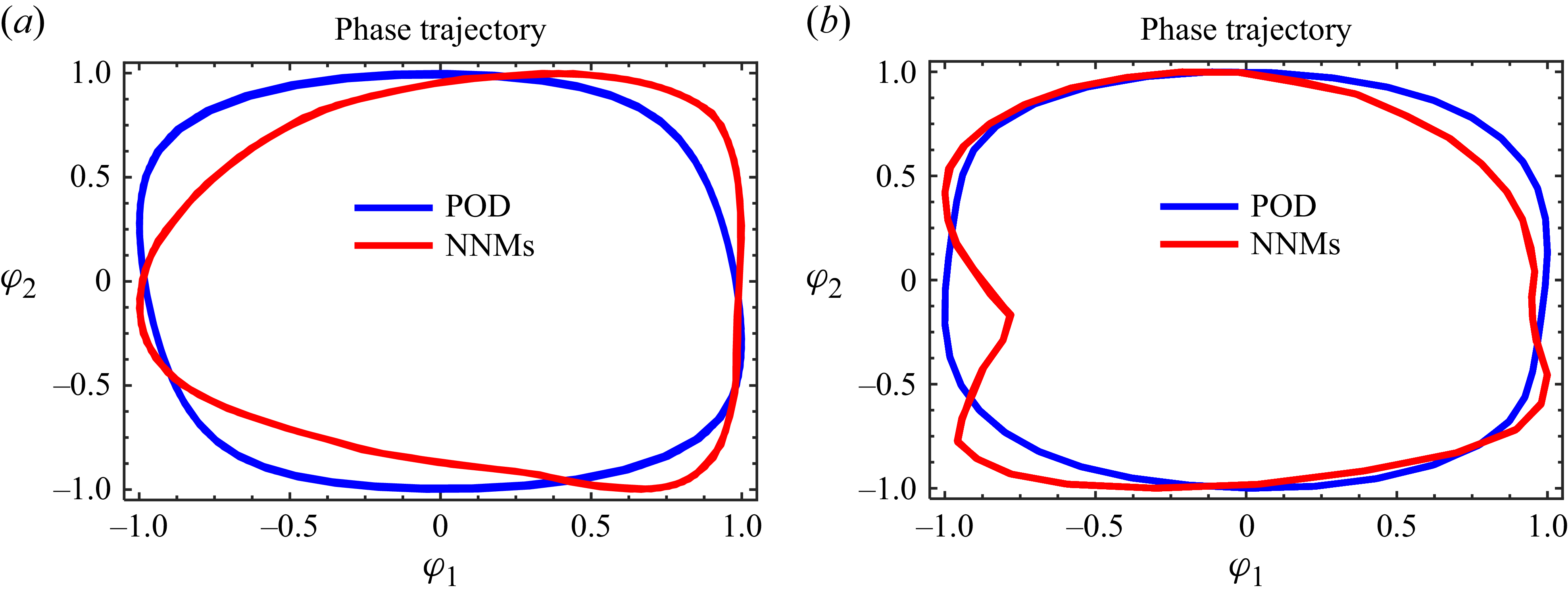
 Re
 Re

 φt
 Vt
 Gfluid
 φt+1,φt+2,…,φk−1,φk
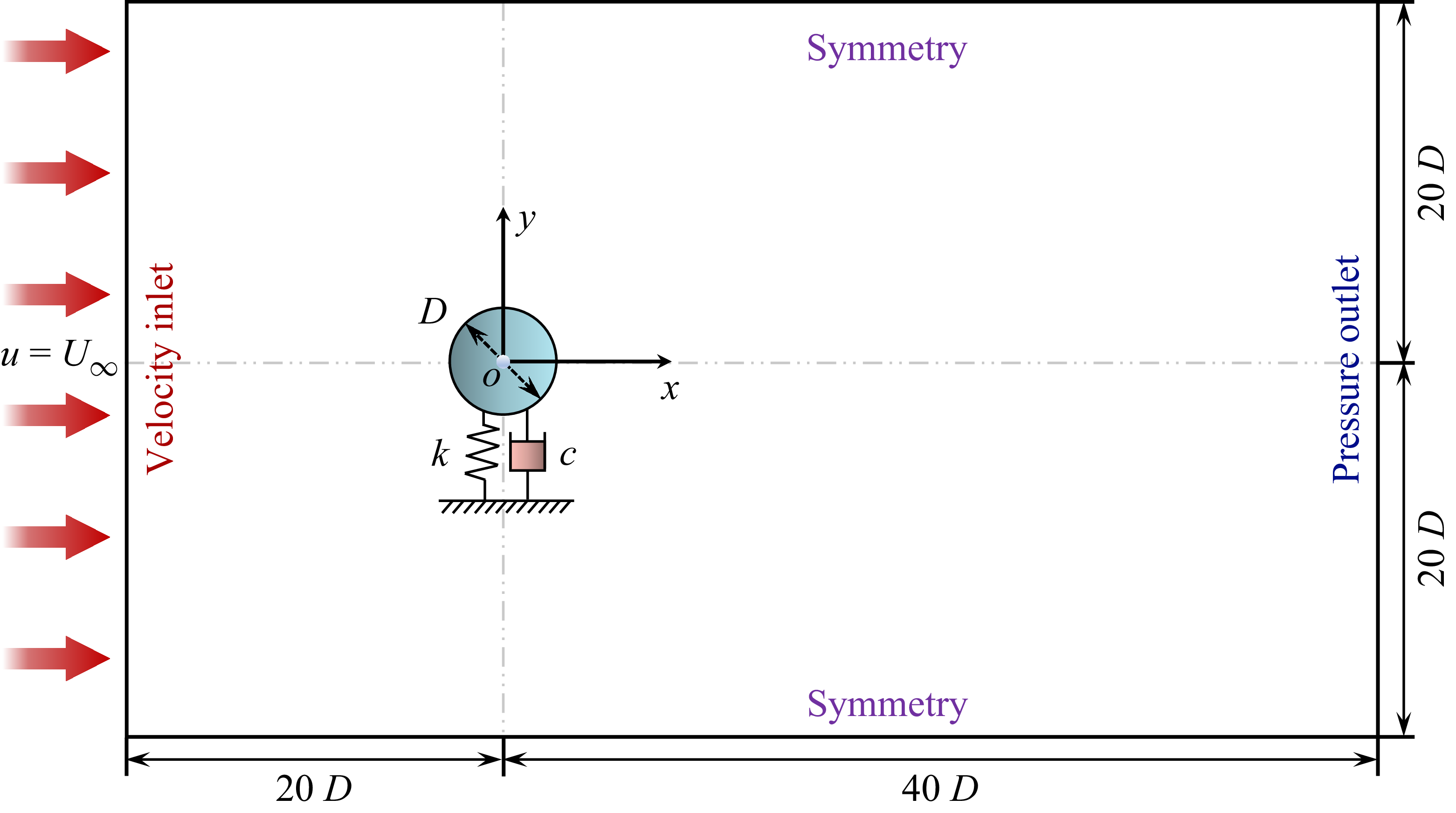


 a
 b
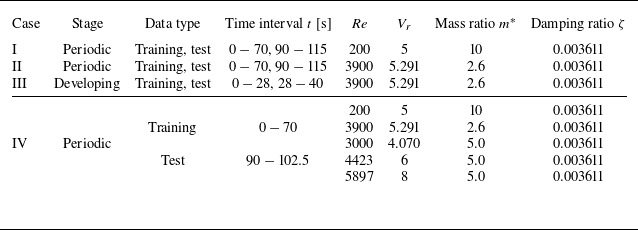
 t

 a
 b
 c
 f∗(=fy/fn)
 m∗=2.6

 Re
 a
 c
 e
 b,d,f

 Re

 Re

 p
 Re

 Re
 a
 b
 c

 Re
 L2
 X/D
 b
 c

 a
 b
 c

 a
 b
 c
 d

 Re
 a
 L2
 b

 Re
 a
 b
 c

 Re
 a
 b
 c

 Re
 L2
 X/D
 a
 b
 c

 Re
 a
 b
 c
 d

 Re
 a
 L2
 b

 Re
 a
 b

 nmode
 b
 c
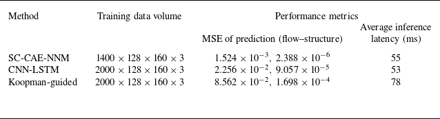
 Re

 Re
 Re
 a
 b
 c
 ωz
 t=10,20
 30


 Re
 a
 c

 ωz
 m∗=5.0
 a
 Vr
 b
 Vr
 c
 Vr

 a
 b

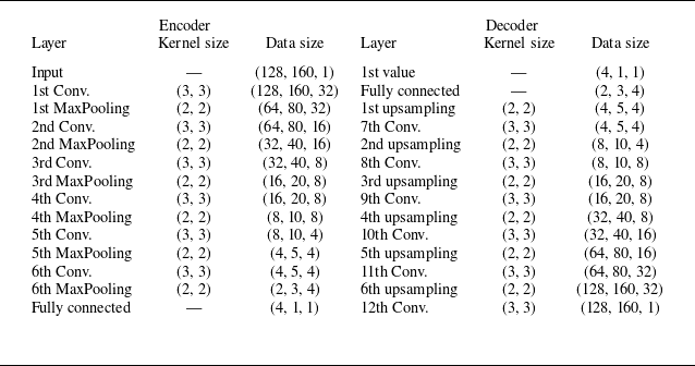

 m∗
 Vr=6
 (Re=4423)


