



1 Introduction
This paper is a continuation of the previous works [Reference Uramoto13, Reference Uramoto15] of the second author, where he studied integral/algebraic Witt vectors and proved the modularity theorem for algebraic Witt vectors over imaginary quadratic fields in particular (Section 2). On the one hand, the (integral/algebraic) Witt vectors studied in [Reference Uramoto13] are those Witt vectors in the sense of Borger [Reference Borger1, Reference Borger2], which are defined over the integer ring
$O_K$
 of a number field K and have their coefficients in algebraic integers; as shown in [Reference Uramoto13], such a Witt vector
$\xi $
 is integral over
$O_K$
 if and only if the orbit under the action of Frobenius lifts is finite (see [Reference Uramoto13, Theorem 3.4]); thanks to the work of Borger and de Smit [Reference Borger and de Smit3, Reference Borger and de Smit4], they are then intrinsically related to the class field theory of K. On the other hand, the modularity theorem for algebraic Witt vectors over imaginary quadratic fields K (see [Reference Uramoto15, Theorems 4.2.1 and 4.3.1) gives an analytic description of the
$\Lambda $
 -ring
${E_K = K \otimes W_{O_K}^a(O_{\bar {K}})}$
 of algebraic Witt vectors over K (where
$W_{O_K}^a(O_{\bar {K}})$
 denotes the
$\Lambda $
 -ring of integral Witt vectors) in terms of the special values of a certain deformation family of Fricke modular functions. The current work belongs in this context and is concerned with a description of
$W_{O_K}^a(O_{\bar {K}})$
 rather than
$E_K = K \otimes W_{O_K}^a(O_{\bar {K}})$
 for imaginary quadratic fields K; to this end, we demonstrate that the modularity theorem provides us a useful symbolic representation of algebraic Witt vectors, with which it is shown that the membership to
$W_{O_K}^a(O_{\bar {K}})$
 within
$E_K$
 is decidable.
Technically, the (strong) modularity theorem (that is, [Reference Uramoto15, Theorem 4.3.1]) shows that (i) the special values of a certain deformation family of Fricke modular functions
$f_a$
 (
$a \in \mathbb {Q}^2/\mathbb {Z}^2$
 ) induce algebraic Witt vectors, which are called modular vectors and denoted
$\widehat {f}_a$
 ; and conversely, (ii) every algebraic Witt vector is generated over K by modular vectors
$\widehat {f}_a$
 (see Section 2). This theorem implies, in particular, that we have a representation of (a priori mysterious) algebraic Witt vectors
$\xi \in E_K$
 over imaginary quadratic fields K as
$\xi = F(\widehat {f}_a)$
 with K-coefficient polynomials
${F(z_a) \in K[z_a \mid a \in \mathbb {Q}^2/\mathbb {Z}^2]}$
 , with which we can manipulate all algebraic Witt vectors symbolically and compute them numerically; thus it makes sense to ask whether the integrality of algebraic Witt vectors
$\xi = F(\widehat {f}_a)$
 is decidable (see Section 2). The major goal of this paper is to show this decidability, providing an effective procedure for determining whether the algebraic Witt vectors
$\xi = F(\widehat {f}_a)$
 belong to
$W_{O_K}^a(O_{\bar {K}})$
 for the polynomials
$F(z_a)$
 ; the proof is based on a module-theoretic argument (see Section 4) together with some estimates of denominators of special values of Fricke functions (see Section 3).
This decidability result gives a natural auxiliary step towards a K-intrinsic/explicit description of the integral Witt vectors among the algebraic ones over imaginary quadratic fields, which was unsolved in [Reference Uramoto15]. In the case of the rational number field
$\mathbb {Q}$
 , it was already shown (see [Reference Uramoto15, Corollary 3.3.1]) that the integral Witt vectors are precisely the
$\mathbb {Z}$
 -linear combinations of the vectors of the form
$\widehat {e}_a := (e^{2 \pi i a \cdot n})_{n\in \mathbb {N}}$
 for
$a \in \mathbb {Q}/\mathbb {Z}$
 ; the proof of this characterization depends on (or is essentially due to) a nontrivial result of Borger and de Smit [Reference Borger and de Smit3, Theorem 3.4]. On the contrary, in the case of imaginary quadratic fields we do not have any satisfactory characterization of integral Witt vectors; in fact, much worse, we do not yet have even nontrivial examples of integral Witt vectors other than the one induced by the j-function (see [Reference Uramoto15, Example 4.1.10]). With this background, the decidability result of this paper enables us to construct and enumerate (in principle all) integral Witt vectors over imaginary quadratic fields, which would also be helpful for formulating some conjectures on a K-intrinsic/expicit characterization of the integral Witt vectors.
The technical challenge for this problem is two-fold. First, in order that an algebraic Witt vector
$\xi $
 is an integral Witt vector, it is necessary that the components
$\xi _{\mathfrak {a}}$
 of
$\xi $
 are all algebraic integers; but from the representation
$\xi = F(\widehat {f}_a)$
 , we can a priori know only approximate numerical values of the components
$\xi _{\mathfrak {a}}$
 . This naively means that we need to judge whether each algebraic number
$\xi _{\mathfrak {a}}$
 is an algebraic integer only from its approximate numerical value. For this first challenge we employ the idea of division polynomials, which tells us necessary upper bounds on the denominators of the special values of Fricke functions
$f_a$
 and is useful to check effectively the integrality of these values (see Section 3).
The second challenge arises from the fact that the integral Witt vectors
$\xi $
 not only have integral components but also must be arithmetically smooth, that is, the distribution of the values
$\xi _{\mathfrak {a}}$
 must be infinitely many differentiable by infinitely many arithmetic derivatives, see Section 2. This arithmetic smoothness is an infinitary condition on
$\xi $
 and a priori impossible to check within finite steps; thus we need to reduce this infinitary condition to some finitary one. For this second challenge, we apply an elementary module-theoretic argument: To be more specific, we prove that
$\xi $
 is arithmetically smooth (that is, infinitely many differentiable) if and only if it is in fact differentiable M times for some number M, where an upper bound of M can be calculated from
$\xi $
 . Technically speaking, this upper bound comes from the fact that a certain K-algebra
$X_\xi $
 induced by
$\xi $
 is finite over K, and thus, the integral closure of
$O_K$
 within
$X_\xi $
 is noetherian; Section 4 is devoted to this second problem and constitutes the central ingredient of this work.
To conclude this paper, we note that, from the decidability of the integral Witt vectors, it also follows, in particular, that the maximal integral models of all galois objects in the semi-galois category
$\mathscr {C}_K$
 of Borger and de Smit [Reference Borger and de Smit3, Reference Borger and de Smit4] for imaginary quadratic fields K can be constructed effectively, for which we devote the last section, Section 5. We also note that no result on numerical computations is provided in this paper; we restrict our attention to the theoretical decidability result. In particular, our algorithm below is not the most efficient one (see Section 4), but instead is designed to be theoretically transparent. Numerical computations would be useful when one formulates some conjectures regarding a description of the integral Witt vectors, which is left open for some future work.
1.1 Related works
We noticed that Borger and de Smit [Reference Borger and de Smit5], following Gurney [Reference Gurney8], had already worked on a related problem in a slightly different form. In particular, in Theorem 11.12, Section 11 [Reference Borger and de Smit5], they gave a description of the maximal integral models of certain galois objects
$X_{\mathfrak {f}}$
 , in terms of (the structure ring of) a Lattes scheme, a coarse moduli space that classifies CM-elliptic curves; and the maximal integral models of the galois objects
$X_{\mathfrak {f}}$
 that they described are isomorphic to the rings of our target objects (that is, integral Witt vectors). In this sense, the current work is strongly related to that of Borger and de Smit [Reference Borger and de Smit5].
It seems however that their characterization itself is not yet completely K-intrinsic nor explicit, unlike the case of
$K = \mathbb {Q}$
 [Reference Borger and de Smit3], and hence does not yet give explicit examples of integral Witt vectors over imaginary quadratic fields. On the other hand, as discussed above too, our decidability result enables us to construct/enumerate by numerical computations all (in principle) integral Witt vectors over imaginary quadratic fields; further, our algorithm is based on the description of algebraic Witt vectors by modular functions on the upper-half space
$\mathfrak {H}$
 (that is, the moduli space of not necessarily CM-elliptic curves; see [Reference Uramoto15, Theorem 4.3.1]), and hence is slightly different also in the setting from [Reference Borger and de Smit5, Reference Gurney8]. In this respect, our decidability result would be complementary to the geometric description of integral Witt vectors due to Borger and de Smit [Reference Borger and de Smit5].
2 Preliminaries
This section gathers from [Reference Borger1–Reference Borger and de Smit4, Reference Uramoto13, Reference Uramoto15] some basic terminology and definitions on algebraic Witt vectors over number fields (Section 2.1) as well as major results concerning the modularity theorem over imaginary quadratic fields (Section 2.2). For more detail and proofs, the reader is referred to the original sources [Reference Borger1–Reference Borger and de Smit4, Reference Uramoto13, Reference Uramoto15]. Essentially this section contains no novel results; the reader who is already familiar with these works can skip directly to the next section, where the major contribution of this work starts.
2.1 Basic definitions
Let K be an arbitrary number field in general and
$O_K$
 the ring of integers in K. We denote by
$P_K$
 the set of nonzero prime ideals of
$O_K$
 , and by
$I_K$
 the monoid of nonzero integral ideals of
$O_K$
 . For each prime
$\mathfrak {p} \in P_K$
 ,
$k_{\mathfrak {p}}$
 denotes the residue field
$k_{\mathfrak {p}} := O_K/ \mathfrak {p}$
 ; and, for each
$\mathfrak {a} \in I_K$
 , its absolute norm is denoted
$N\mathfrak {a}$
 .
The major object of this work concerns the ring
$W_{O_K}(A)$
 of (generalized) Witt vectors over
$O_K$
 with components in an
$O_K$
 -algebra A introduced by Borger [Reference Borger1, Reference Borger2]; for our purpose, we only need to recall the definition of
$W_{O_K}(A)$
 for a flat
$O_K$
 -algebra A, in particular. In what follows, we denote by
$A^{I_K}$
 the
$I_K$
 -times product of A; and by
$\psi _{\mathfrak {c}}: A^{I_K} \rightarrow A^{I_K}$
 for
$\mathfrak {c} \in I_K$
 the
$\mathfrak {c}$
 -shift operator defined by
$\psi _{\mathfrak {c}} (\xi ) := (\xi _{\mathfrak {c} \mathfrak {a}})_{\mathfrak {a}}$
 for each
$\xi = (\xi _{\mathfrak {a}})_{\mathfrak {a}} \in A^{I_K}$
 . Informally speaking, the ring
$W_{O_K}(A)$
 of Witt vectors is defined as a subring of
$A^{I_K}$
 consisting of those
$\xi \in A^{I_K}$
 that are smooth with respect to arithmetic derivatives (in the sense of Remark 2.2 below).
Definition 2.1 (the ring
$W_{O_K}(A)$
 of Witt vectors).

Let A be a flat
$O_K$
 -algebra. Then the ring
$W_{O_K}(A)$
 of Witt vectors over
$O_K$
 with components in A is defined as the intersection
$\bigcap _n U_n(A)$
 of the following subalgebras
$U_n (A) \subseteq A^{I_K}$
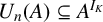 defined by induction on
$n \geq 0$
 :

Remark 2.2 (arithmetic smoothness of Witt vectors).
To gain some intuition on Witt vectors, it is helpful to review the above definition for the case where K is of class number one, in particular; in fact, informally speaking, the above ring
$U_n(A) \subseteq A^{I_K}$
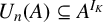 can be regarded as the ring of ‘
$C^n$
 -functions’ on
$I_K$
 with respect to arithmetic derivatives in the sense of Buium [Reference Buium6], whence
$W_{O_K}(A) = \bigcap _n U_n(A)$
 is then regarded as the ring of ‘
$C^\infty $
 -functions’ on
$I_K$
 .
When K is of class number one, we can take a uniformizer
$\pi _{\mathfrak {p}} \in \mathfrak {p}$
 for each prime
$\mathfrak {p} \in P_K$
 so that
$\mathfrak {p} = \pi _{\mathfrak {p}} O_K$
 ; then the above inductive definition of
$U_{n+1}(A)$
 means that
$\xi \in U_n(A)$
 belongs to
$U_{n+1}(A)$
 if and only if
$(\psi _{\mathfrak {p}} \xi - \xi ^{N\mathfrak {p}})/\pi _{\mathfrak {p}} \in U_n(A)$
 for all
$\mathfrak {p}$
 . Here the operator
$\xi \mapsto (\psi _{\mathfrak {p}} \xi - \xi ^{N\mathfrak {p}})/\pi _{\mathfrak {p}}$
 was studied by Buium [Reference Buium6] as an analogue of the usual derivation
$f(z) \mapsto \lim _{h \to 0} (f(z+h) - f(z))/h$
 of functions, and called the arithmetic derivation; we denote this operation as
$\delta _{\mathfrak {p}} \xi := (\psi _{\mathfrak {p}} \xi - \xi ^{N\mathfrak {p}})/\pi _{\mathfrak {p}}$
 . With this analogy in mind, if we regard
$U_0(A)$
 as the ring of ‘continuous functions’ on
$I_K$
 , the ring
$U_n(A)$
 can be inductively regarded as that of ‘
$C^n$
 -functions’ in the sense of these arithmetic derivatives
$\delta _{\mathfrak {p}}$
 . It is in this sense that we regard the ring
$W_{O_K}(A) = \bigcap _n U_n(A)$
 of Witt vectors as that of ‘
$C^\infty $
 -functions’; moreover, by comparing it with the arithmetic derivative
$\delta _{\mathfrak {p}} \xi = (\psi _{\mathfrak {p}} \xi - \xi ^{N\mathfrak {p}})/\pi _{\mathfrak {p}}$
 , the
$\mathfrak {p}$
 -shift operator
$\psi _{\mathfrak {p}}$
 for each prime
$\mathfrak {p}$
 can also be regarded as a kind of ‘difference operator’.
In general the ring
$W_{O_K}(A)$
 of Witt vectors enjoys the following properties, which means that
$W_{O_K}(A)$
 is not just a ring but in fact has a structure of a (generalized)
$\Lambda $
 -ring [Reference Borger1].
Proposition 2.3 (Borger, [Reference Borger1, Proposition 1.9]).
The ring
$W_{O_K}(A)$
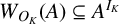
 satisfies the following properties: for all
$\xi \in W_{O_K}(A)$
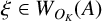 and
$\mathfrak {p}, \mathfrak {q} \in P_K$
 ,
-
(1) $\psi _{\mathfrak {p}} \xi \in W_{O_K}(A)$
, that is,
$W_{O_K}(A) \subseteq A^{I_K}$
is closed under
$\psi _{\mathfrak {p}}: A^{I_K} \rightarrow A^{I_K}$
; -
(2) $\psi _{\mathfrak {p}} \psi _{\mathfrak {q}} = \psi _{\mathfrak {q}} \psi _{\mathfrak {p}}$
, that is,
$\psi _{\mathfrak {p}}$
s commute with each other; -
(3) $\psi _{\mathfrak {p}} \xi - \xi ^{N\mathfrak {p}} \in \mathfrak {p} W_{O_K}(A)$
, that is,
$\psi _{\mathfrak {p}}$
lifts the Frobenius map on
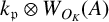
$k_{\mathfrak {p}} \otimes W_{O_K}(A)$
onto
$W_{O_K}(A)$
.






Remark 2.4 (generalized
$\Lambda $
-ring).

In general, a (flat)
$O_K$
 -algebra A is said to be a
$\Lambda $
 -ring if A is equipped with a mutually commuting family
$\{\psi _{\mathfrak {p}}: A \rightarrow A\}$
 of
$O_K$
 -algebra homomorphisms such that
$\psi _{\mathfrak {p}} a - a^{N\mathfrak {p}} \in \mathfrak {p} A$
 for all
$a \in A$
 and
$\mathfrak {p} \in P_K$
 . In this sense, the ring
$W_{O_K}(A)$
 of Witt vectors is an example of
$\Lambda $
 -rings. In fact, the construction
$A \mapsto W_{O_K}(A)$
 extends to a comonad
$W_{O_K}$
 on the category of (not necessarily flat)
$O_K$
 -algebras; and the
$\Lambda $
 -rings are defined in general as comodules
$\nabla : A \rightarrow W_{O_K}(A)$
 for this comonad
$W_{O_K}$
 . In particular, the ring
$W_{O_K}(A)$
 of Witt vectors is the cofree
$\Lambda $
 -ring (that is, the cofree comodule
$W_{O_K}(A) \rightarrow W_{O_K}(W_{O_K}(A))$
 with respect to this comonad
$W_{O_K}$
 ). See [Reference Borger1] for more detail.
Amongst (generalized) Witt vectors, our major concern is with the integral Witt vectors over
$O_K$
 with coefficients in the algebraic integers
$O_{\bar {K}}$
 , in particular; the algebraic Witt vectors over K are also of our central concern, being defined through integral Witt vectors as follows.
Definition 2.5 (integral and algebraic Witt vectors).
We say that a Witt vector
${\xi \in W_{O_K}(O_{\bar {K}})}$
 is an integral Witt vector over
$O_K$
 if it is integral over
$O_K$
 ; we denote simply by
$A_K$
 the subring of
$W_{O_K}(O_{\bar {K}})$
 consisting of integral Witt vectors (which coincides with
$W_{O_K}^a(O_{\bar {K}})$
 in [Reference Uramoto13]). Moreover, by the algebraic Witt vectors over K we mean the elements of
$E_K:= K \otimes A_K$
 .
Remark 2.6 (
$A_K$
and
$E_K$
are
$\Lambda $
-rings).


It can be shown that the subring
${A_K \subseteq W_{O_K}(O_{\bar {K}})}$
 is also a
$\Lambda $
 -ring with respect to the restriction of the Frobenius lifts
$\psi _{\mathfrak {p}}: W_{O_K}(O_{\bar {K}}) \rightarrow W_{O_K}(O_{\bar {K}})$
 onto
$A_K$
 ; this is also the case for
$E_K = K \otimes A_K$
 , which is equipped with the action of
$\psi _{\mathfrak {p}}$
 s induced from those on
$A_K$
 . See [Reference Uramoto13, Section 3.2] for more detail.
By definition, an (integral) Witt vector
$\xi \in A_K$
 is a vector
$\xi = (\xi _{\mathfrak {a}})$
 that consists of algebraic integers
$\xi _{\mathfrak {a}} \in O_{\bar {K}}$
 indexed by the nonzero integral ideals
$\mathfrak {a} \in I_K$
 such that the distribution of the values
$\xi _{\mathfrak {a}}$
 on
$I_K$
 is arithmetically smooth; when K is of class number one, in particular, this means that the rth arithmetic derivatives
$\delta _{\mathfrak {p}_1} \cdots \delta _{\mathfrak {p}_r} \xi $
 of
$\xi $
 must have integral components for any
$r \geq 0$
 and any
$\mathfrak {p}_1, \ldots , \mathfrak {p}_r \in P_K$
 . In view of the fact that the arithmetic derivative
$\delta _{\mathfrak {p}} \xi = (\psi _{\mathfrak {p}} \xi - \xi ^{N\mathfrak {p}})/\pi _{\mathfrak {p}}$
 contains the fractional operation
$\pi _{\mathfrak {p}}^{-1}$
 , the arithmetic smoothness of
$\xi \in A_K$
 (that the components of
$\delta _{\mathfrak {p}_1} \cdots \delta _{\mathfrak {p}_r} \xi $
 must be all integers) imposes a strong constraint on the distribution of the integral values
$\xi _{\mathfrak {a}}$
 . In fact, for instance, the components
$\xi _{\mathfrak {a}}$
 of
$\xi \in A_K$
 are all forced to be abelian over K, despite the fact that we only assume that the
$\xi _{\mathfrak {a}}$
 s are algebraic integers (hence, a priori not necessarily abelian over K); see [Reference Borger and de Smit4, Section 3] and [Reference Uramoto13, Section 4].
Yet another constraint imposed on integral Witt vectors
$\xi \in A_K$
 is that the orbit of
$\xi $
 under the action of the operators
$\psi _{\mathfrak {p}}$
 (or Frobenius lifts) is finite; in fact, this orbit-finiteness characterizes the integral Witt vectors
$\xi \in A_K$
 among general Witt vectors in
$W_{O_K}(O_{\bar {K}})$
 . In what follows, note that if an integral ideal
$\mathfrak {a} \in I_K$
 decomposes as
$\mathfrak {a} = \mathfrak {p}_1 \cdots \mathfrak {p}_n$
 , the operator
$\psi _{\mathfrak {a}}$
 is equal to the composition
$\psi _{\mathfrak {p}_1} \circ \cdots \circ \psi _{\mathfrak {p}_n}$
 of the Frobenius lifts
$\psi _{\mathfrak {p}_i}$
 .
Theorem 2.7 (arithmetic Christol theorem [Reference Uramoto13]).
A Witt vector
$\xi \in W_{O_K}(O_{\bar {K}})$
 is integral over
$O_K$
 if and only if the orbit
$I_K \xi := \{\psi _{\mathfrak {a}} \xi \mid \mathfrak {a} \in I_K\}$
 under the action of
$\psi _{\mathfrak {a}}$
 s is a finite set, and also, if and only if the set
$C_\xi := \{\xi _{\mathfrak {a}} \mid \mathfrak {a} \in I_K\}$
 of the component values
$\xi _{\mathfrak {a}}$
 of
$\xi $
 is a finite set.
Due to this strong constraint on the components
$\xi _{\mathfrak {a}}$
 , only a few examples of integral Witt vectors have been explicitly constructed so far; the few examples include those over
$\mathbb {Z}$
 [Reference Uramoto15, Corollary 3.3.1] and the one induced by the j-function [Reference Uramoto15, Example 4.1.10]. This fact motivates the current work; and the subject of this paper is to give at least an effective algorithm to enumerate (in principle all) examples of integral Witt vectors over imaginary quadratic fields. For this purpose, the modularity theorem for algebraic Witt vectors [Reference Uramoto15] gives us a useful representation of algebraic Witt vectors as we briefly recall below.
2.2 The modularity theorem
Unlike the case of integral Witt vectors, we have a relatively concise description of algebraic Witt vectors; in particular, in the case of imaginary quadratic fields K, the distribution of the components
$\xi _{\mathfrak {a}}$
 of algebraic Witt vectors
$\xi \in E_K$
 admits an analytic description in terms of special values of a deformation family of Fricke functions
$f_a$
 (indexed by
$a=(a_1, a_2) \in \mathbb {Q}^2/\mathbb {Z}^2$
 ), which are modular functions on the upper-half plane
$\mathfrak {H} :=\{z \in \mathbb {C} \mid \mathrm {Im}(\tau )> 0\}$
 . Here we recall the definition of the Fricke functions
$f_a$
 (see [Reference Shimura11]), with which the modular vectors
$\widehat {f}_a$
 are constructed.
Definition 2.8 (Fricke functions
$f_a$
).

Let K be an imaginary quadratic field. The Fricke function
$f_a$
 indexed by
$a = (a_1, a_2) \in \mathbb {Q}^2/\mathbb {Z}^2$
 with
$a \neq 0$
 is defined as follows: for each
$\tau \in \mathfrak {H}$
 ,

for
$a=0$
 we define
$f_0(\tau ) = j(\tau )$
 with the j-function j; also,
$\wp $
 is the Weierstrass
$\wp $
 -function.
As shown in [Reference Uramoto15] this family of modular functions
$f_a$
 induces algebraic Witt vectors
$\widehat {f}_a$
 in a certain manner; technically, this construction is based on a canonical isomorphism between the
$\Lambda $
 -ring
$E_K$
 of algebraic Witt vectors and the
$\Lambda $
 -ring
$\mathrm {Hom}_{G_K}(DR_K, K^{ab})$
 of locally constant,
$K^{ab}$
 -valued,
$G_K$
 -equivariant functions on a profinite monoid
$DR_K$
 called the Deligne–Ribet monoid [Reference Uramoto15, Corollary 3.1.6]; this profinite monoid
$DR_K$
 is defined as the inverse limit of the following finite Deligne–Ribet monoids (or the ray class monoids).
Definition 2.9 (ray class monoid
$DR_{\mathfrak {f}}$
, [Reference Deligne and Ribet7]).

For each
$\mathfrak {f} \in I_K$
 , we define the finite Deligne–Ribet monoid
$DR_{\mathfrak {f}}$
 (or the ray class monoid of conductor
$\mathfrak {f}$
 ) as the finite quotient
$DR_{\mathfrak {f}} := I_K/\sim _{\mathfrak {f}}$
 of the monoid
$I_K$
 with respect to the following congruence
$\sim _{\mathfrak {f}}$
 of finite index: for
$\mathfrak {a}, \mathfrak {b} \in I_K$
 ,

where
$K^+$
 denotes the totally positive elements of K.
Remark 2.10 (definition and structure of
$DR_K$
).

It is known from [Reference Deligne and Ribet7] that (i) for
$\mathfrak {f} \mid \mathfrak {f}'$
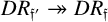
 , we have a canonical surjective monoid homomorphism
$DR_{\mathfrak {f}'} \twoheadrightarrow DR_{\mathfrak {f}}$
 ; and (ii) the unit group
$DR_{\mathfrak {f}}^\times $
 is naturally isomorphic to the (strict) ray class group
$C_{\mathfrak {f}}$
 for conductor
$\mathfrak {f}$
 . Thus, by (i), the finite monoids
$DR_{\mathfrak {f}}$
 constitute an inverse system, whose inverse limit is the Deligne–Ribet monoid
$DR_K$
 ; moreover, from (ii), it also follows that the unit group
$DR_K^\times $
 is isomorphic to the maximal abelian Galois group
$G_K^{ab}$
 by class field theory. This way,
$DR_K$
 admits a natural
$G_K$
 -action via
$G_K \twoheadrightarrow G_K^{ab} \simeq DR_K^\times \hookrightarrow DR_K$
 ; note also that, as each
$DR_{\mathfrak {f}}$
 is a finite quotient of
$I_K$
 , we have a canonical homomorphism
$I_K \rightarrow DR_K$
 , which is in fact injective and has a dense image.
Since
$DR_K$
 has an action of
$G_K$
 , we may consider locally constant
$K^{ab}$
 -valued
$G_K$
 -equivariant functions on
$DR_K$
 , the set of which is denoted by
$\mathrm {Hom}_{G_K}(DR_K, K^{ab})$
 and forms a K-algebra with respect to the point-wise operations. Moreover, since
$I_K$
 embeds into
$DR_K$
 , we also have mutually commuting operators
$\psi _{\mathfrak {p}}: \mathrm {Hom}_{G_K}(DR_K, K^{ab}) \rightarrow \mathrm {Hom}_{G_K}(DR_K, K^{ab})$
 defined by
$\psi _{\mathfrak {p}} \xi (x) := \xi (\mathfrak {p} x)$
 for each
$\xi \in \mathrm {Hom}_{G_K}(DR_K, K^{ab})$
 and
$x \in DR_K$
 . With these structures,
$\mathrm {Hom}_{G_K}(DR_K, K^{ab})$
 forms a
$\Lambda $
 -ring, which is in fact isomorphic to
$E_K$
 .
Theorem 2.11 [Reference Uramoto15, Corollary 3.1.6].
We have a canonical isomorphism of
$\Lambda $
 -rings:

This theorem says that, to construct algebraic Witt vectors, it is sufficient to construct locally constant
$K^{ab}$
 -valued
$G_K$
 -equivariant functions on
$DR_K$
 ; our construction of modular vectors
$\widehat {f}_a$
 is based on this fact, together with the presentation of
$DR_K$
 due to Yalkinoglu [Reference Yalkinoglu17]; in this paper, we need this presentation for the case of imaginary quadratic fields, which is given as follows.
Proposition 2.12 (Yalkinoglu, [Reference Yalkinoglu17, Proposition 8.2]).
Let K be an imaginary quadratic field. Then we have a canonical isomorphism of profinite monoids:

where the monoid
$\widehat {O}_K \times _{\widehat {O}_K^\times } (\mathbb {A}_{K, f}^\times /K^\times )$
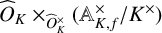 is the quotient of the multiplicative monoid
${\widehat {O}_K \times (\mathbb {A}_{K, f}^\times /K^\times )}$
 by the action of the group
$\widehat {O}_K^\times $
 given by
$[\rho , s] \mapsto [\rho u, u^{-1} s]$
 for each
$u \in \widehat {O}_K^\times $
 .
With these preparations, we now recall the construction of modular vectors
$\widehat {f}_a$
 over imaginary quadratic fields K (see [Reference Uramoto15, Section 4.1]). Below, throughout this paper, K denotes an imaginary quadratic field. The following definition first gives a general construction of
$\widehat {f}_a$
 ; for more detail the reader is referred to [Reference Uramoto15]; but we then recall a more explicit description of this construction given by [Reference Uramoto15, Lemma 4.1.9], which would be more useful for actual computations.
Definition 2.13 (modular vector
$\widehat {f}_a$
).

Let K be an imaginary quadratic field; for each
$a \in \mathbb {Q}^2/\mathbb {Z}^2$
 , the modular vector
$\widehat {f}_a: DR_K \rightarrow K^{ab}$
 is defined as follows:

where
$\rho \in \widehat {O}_K$
 acts on
$a \in \mathbb {Q}^2/\mathbb {Z}^2$
 via the natural isomorphisms
$\mathbb {Q}^2/\mathbb {Z}^2 \simeq K/O_K \simeq \mathbb {A}_{K, f}/ \widehat {O}_K$
 , the first one being determined by a basis of the
$\mathbb {Z}$
 -module
$O_K = \mathbb {Z} \tau _K + \mathbb {Z}, \tau _K \in \mathfrak {H}$
 ; this basis also induces an adelic representation
$q: \mathbb {A}_{K, f} \rightarrow \mathrm {GL}_2(\mathbb {A}_{\mathbb {Q}, f})$
 , so that
$q(s) \in \mathrm {GL}_2(\mathbb {A}_{\mathbb {Q}, f})$
 admits a decomposition of the form
$q(s) = u \cdot \alpha _s$
 , where
$u \in \mathrm {GL}_2(\widehat {\mathbb {Z}})$
 and
$\alpha _s \in \mathrm {GL}_2(\mathbb {Q})$
 . The former
$u \in \mathrm {GL}_2(\widehat {\mathbb {Z}})$
 naturally acts on
$\mathbb {Q}^2/\mathbb {Z}^2 \simeq \mathbb {A}_{\mathbb {Q}, f}^2/ \widehat {\mathbb {Z}}^2$
 ; the latter
$\alpha _s$
 determines
$\tau _s \in \mathfrak {H}$
 as the usual fractional transformation
$\tau _s := \alpha _s(\tau _K)$
 .
Remark 2.14. The above construction of modular vectors has a natural geometric interpretation, which is related to the fact that the special values of Fricke functions are x-coordinates of torsion points of elliptic curves; see, for example, [Reference Shimura11, Section 4.5]. In a sequel work [Reference Uramoto16] of [Reference Uramoto15], the second author has clarified this geometric interpretation of modular vectors in more detail in relation to an extension of [Reference Uramoto15] to the case of CM fields. For this geometric viewpoint, the interested reader is referred to [Reference Uramoto16, Section 2.1.2], in particular.
Theorem 2.15 (modularity theorem, [Reference Uramoto15, Theorem 4.3.1]).
For each
$a \in \mathbb {Q}^2/\mathbb {Z}^2$
 , the modular vector
$\widehat {f}_a$
 defines a locally constant
$K^{ab}$
 -valued
$G_K$
 -equivariant function on
$DR_K$
 , hence gives an algebraic Witt vector
$\widehat {f}_a \in E_K$
 ; moreover, these modular vectors generate
$E_K$
 over K. That is,

This theorem means that every algebraic Witt vector
$\xi $
 can be represented as
$\xi = F(\widehat {f}_a)$
 with a K-coefficient polynomial
$F(z_a) \in K[z_a \mid a \in \mathbb {Q}^2/\mathbb {Z}^2]$
 . Since the coefficients of
$F(z_a)$
 are all in
$K = \mathbb {Q} \tau _K + \mathbb {Q}$
 , each polynomial
$F(z_a)$
 can be identified with the finitely many rational numbers appearing in its coefficients, which enables us to manipulate all algebraic Witt vectors
$\xi = F(\widehat {f}_a)$
 symbolically. With this representation, it makes sense to ask the decidability of whether a given algebraic Witt vector
$\xi = F(\widehat {f}_a) \in E_K$
 belongs to
$A_K$
 ; and the main result of this paper is to prove this decidability.
Theorem 2.16 (decidability of integral Witt vectors).
It is decidable whether a given
$\xi = F(\widehat {f}_a) \in E_K$
 belongs to
$A_K \subset E_K$
 for the polynomial
$F(z_a)$
 .
As mentioned above, the function
$\widehat {f}_a: DR_K \rightarrow K^{ab}$
 induces an algebraic Witt vector actually by restricting this function onto its submonoid
$I_K \hookrightarrow DR_K$
 . In the current case, K being imaginary quadratic, this restriction can be calculated by [Reference Uramoto15, Lemma 4.1.9] more explicitly as follows.
Proposition 2.17 (see [Reference Uramoto15, Lemma 4.1.9]).
Let
$K=\mathbb {Q}(\sqrt {-d})$
 with a square-free natural number d; represent each nonzero integral ideal
$\mathfrak {a} \in I_K$
 as
$\mathfrak {a} = \mathbb {Z} (a \tau _K + b) + \mathbb {Z} c$
 with integers
$a, b, c \in \mathbb {Z}$
 . Then the
$\mathfrak {a}$
 th component of
$\widehat {f}_a \in E_K$
 is given as follows:

where
$\beta \in \mathrm {GL}_2(\mathbb {Z})$
 is determined by
$\mathfrak {a}^{-1} = \mathbb {Z}^2 \cdot \beta \cdot (\tau _K, 1)^t = \mathbb {Z} w_1 + \mathbb {Z} w_2$
 so that
${\tau _{\mathfrak {a}^{-1}} = w_1/w_2 \in \mathfrak {H}}$
 . In particular,

Proof. By [Reference Uramoto15, Lemma 4.1.9], we have
$\widehat {f}_a (\mathfrak {a}) = f_{a \cdot \beta ^{-1}} (\tau _{\mathfrak {a}^{-1}})$
 , where
$\mathfrak {a}^{-1} = \mathbb {Z}^2 \cdot \beta \cdot (\tau _K, 1)^t = \mathbb {Z} w_1 + \mathbb {Z} w_2$
 for
$\beta \in M_2(\mathbb {Q})$
 and
$\tau _{\mathfrak {a}^{-1}} = w_1 / w_2$
 . Here, the matrix
$\beta $
 can be computed more explicitly using the equalities
$\mathfrak {a}^{-1} = (N\mathfrak {a})^{-1} \bar {\mathfrak {a}}$
 and
$N\mathfrak {a} = ac$
 , where
$\bar {\mathfrak {a}}$
 is the Galois conjugate of
$\mathfrak {a}$
 ; thus,

From this, the inverse
$\beta ^{-1}$
 can be computed as Equation (2-1), hence the claim.
Now we proceed to the problem of judging the integrality of algebraic Witt vectors. As outlined in Section 1, the major technical challenge is two-fold. First, we need to check whether each component
$\xi _{\mathfrak {a}}$
 of an algebraic Witt vector
$\xi = F(\widehat {f}_a) \in E_K$
 is an algebraic integer, which is the subject of Section 3; for this task, we employ the idea of division polynomials [Reference Silverman12] from the theory of elliptic curves. As remarked in Section 1 too, nevertheless, in order that
$\xi \in E_K$
 is an integral Witt vector (that is,
$\xi \in A_K$
 ), it is not sufficient that every component
$\xi _{\mathfrak {a}}$
 of
$\xi $
 is an algebraic integer: the distribution of the integers
$\xi _{\mathfrak {a}}$
 must be smooth with respect to arithmetic derivations, namely, infinitely differentiable by any
$\mathfrak {p} \in P_K$
 . The subject of Section 4 is thus to develop an effective procedure of checking this arithmetic smoothness, based on an elementary module-theoretic idea.
3 Integrality of components
The subject of this section is to prove that it is decidable whether the component
$\xi _{\mathfrak {a}}$
 of an algebraic Witt vector
$\xi \in E_K$
 at each ideal
$\mathfrak {a} \in I_K$
 is an algebraic integer; since every
$\xi \in E_K$
 is represented as
$\xi = F(\widehat {f}_a)$
 , this decidability is reduced to giving an estimate of the denominators of the special value of the Fricke functions
$f_a$
 at each imaginary quadratic point
$\tau \in \mathfrak {H}$
 . This decidability is needed in our target decision procedure developed in the next section (Section 4).
3.1 Outline of algorithm
The Fricke functions
$f_a$
 , used in the construction of the above modular vectors
$\widehat {f}_a \in E_K$
 , are defined in terms of Eisenstein series (see [Reference Shimura11]); hence, we can compute the components
$\widehat {f}_a(\mathfrak {a})$
 of the modular vectors
$\widehat {f}_a \in E_K$
 (= special values of
$f_a$
 s), and therefore those of all
$\xi \in E_K$
 as well, approximately with an arbitrary accuracy. The problem here is to judge whether the components
$\xi _{\mathfrak {a}}$
 of
$\xi = F(\widehat {f}_a)$
 are integers, using only this approximate numerical value.
Concerning this issue, note first that, for any
$\xi = F(\widehat {f}_a) \in E_K$
 , the indices
$a \in \mathbb {Q}^2/\mathbb {Z}^2$
 appearing in the polynomial
$F(z_a) \in K[z_a \mid a\in \mathbb {Q}^2/\mathbb {Z}^2]$
 are in
$N^{-1} \mathbb {Z}^2/\mathbb {Z}^2$
 for some natural number
$N \geq 1$
 , whence the components
$\xi _{\mathfrak {a}}$
 of
$\xi \in E_K$
 all belong in the ray class field
$K_{NO_K}$
 with the conductor
$NO_K \in I_K$
 ; in fact, this result can be stated more specifically as follows.
Proposition 3.1 (see [Reference Uramoto15, Proposition 3.2.1 and Lemma 4.3.5]).
For each
${a \in N^{-1}\mathbb {Z}^2/\mathbb {Z}^2}$
 , we have
$\widehat {f}_a \in X_{NO_K} \simeq \prod _{\mathfrak {d} \mid NO_K} K_{NO_K / \mathfrak {d}}$
 .
Therefore, the integrality of
$\xi _{\mathfrak {a}}$
 s can be judged by checking the integrality of the symmetric functions
$s(\xi _{\mathfrak {a}}^{\sigma } \mid \sigma \in \mathrm {Gal}(K_{NO_K}/K)) \in K$
 of the conjugates of
$\xi _{\mathfrak {a}} \in K_{NO_K}$
 over K, at least whose values are computable by Proposition 2.17. Of course, as mentioned above too, we can know only approximate values of
${s = s(\xi _{\mathfrak {a}}^{\sigma } \mid \sigma \in \mathrm { Gal}(K_{NO_K}/K)) \in K}$
 ; but if we could estimate upper bounds of their denominators, we can judge the integrality of such values s since we know that the (for example, decimal) expansions of
$s_1, s_2$
 where
$s = s_1 + s_2 \tau _K$
 with
$O_K = \mathbb {Z} + \mathbb {Z} \tau _K$
 are periodic (because
$s_1, s_2 \in \mathbb {Q}$
 ), and that the periods can be estimated by the size of the denominator of s; also we can compute their decimal expansions in any accuracy.
Moreover, since all
$\xi \in E_K$
 are expressed as K-polynomials of
$\widehat {f}_a$
 s, we can estimate the upper bound of the denominator of the above s for all
$\xi \in E_K$
 if we could do this just for the special values of
$f_a$
 s at imaginary quadratic
$\tau \in \mathfrak {H}$
 . As seen in Definition 2.8, these special values are constant multiples of x-coordinates of torsion points in an elliptic curve for
$\tau $
 ; hence, the problem is reduced to an estimate of the denominators of coordinates of torsion points on elliptic curves, for which, however, some more information on arithmetic of elliptic curves is needed. Indeed we then solve this problem by employing the idea of division polynomials from the theory of elliptic curves (see [Reference Silverman12]); in fact, division polynomials are explicitly computable and tell us polynomials whose roots are the special values of
$f_a$
 s, hence are useful to give upper bounds of their denominators. Therefore, using this, we can judge the integrality of the components of the modular vectors
$\widehat {f}_a$
 (
$a \in \mathbb {Q}^2/\mathbb {Z}^2$
 ), hence the integrality of the components
$\xi _{\mathfrak {a}}$
 of any
$\xi = F(\widehat {f}_a) \in E_K$
 as well.
3.2 Estimate of denominators
Before stating, we first recall the definition of division polynomials from [Reference Silverman12, Exercise III.3.7]. Let
$E \colon y^2 = x^3 - Ax - B$
 be an elliptic curve over a number field k. For
$n \ge 0$
 , the division polynomial
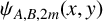
$\psi _{A, B, n} = \psi _{A, B, n}(x, y) \in \mathbb {Z}[A, B, x, y]$
 is defined by the following recurrence equation for
$m \ge 2$


with initial conditions

Putting
$\deg x = 2, \deg y = 3, \deg A = 4$
 and
$\deg B = 6$
 , we can derive the following properties of these division polynomials
$\psi_{A, B, N} (x, y)$
 .
Lemma 3.2 [Reference Silverman12, Exercise III.3.7].
For
$N \ge 1$
 , the polynomial
$\psi _{A, B, N}(x,y)$
 is homogeneous of degree
$N^2-1$
 . Moreover, the following hold:
-
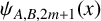
(1) If $N = 2m+1$
, then
$\psi _{A, B, 2m+1}$
is a polynomial in
$\mathbb {Z}[x, A, B]$
. -
(2) If $N = 2m$
, then
$\psi _{A, B, 2m}(x,y)$
is divisible by
$2y$
, and the quotient is a polynomial in
$\mathbb {Z}[x, A, B]$
. -
(3) In each case, the term of highest degree as a polynomial of $x, y$
is uniquely determined;
$Nx^{2m^2 + 2m}$
if
$N = 2m + 1$
, and
$Nx^{2m^2 + 4m} y$
if
$N = 2m+2$
. In particular, the coefficient is N.







Moreover, we find the following description.
Lemma 3.3 [Reference Silverman12, Exercise III.3.7].
-
(1) For $N = 2m+1$
with
$m \ge 1$
, $$ \begin{align*} \psi_{A, B, 2m+1}(x) = (2m+1) \prod_{ \substack{P \in E_{A,B}[2m+1]/\pm \\ P \neq O}} (x - x(P)). \end{align*} $$In other words, the zeros of division polynomial $\psi _{A, B, 2m+1}(x)$
are the x-coordinates of nontrivial
$(2m+1)$
-torsion points of
$E_{A, B}$
.
-
(2) For $N = 2m+2$
with
$m \ge 1$
, $$ \begin{align*} \psi_{A, B, 2m+2}(x, y) = 2y \cdot (m+1) \prod_{ \substack{P \in E_{A,B}[2m+2]/\pm \\ 2P \neq O}} (x - x(P)). \end{align*} $$In other words, the zeros of division polynomial $\psi _{A, B, 2m+2}(x, y)/2y$
are the x-coordinates of
$(2m+2)$
-torsion points of
$E_{A, B}$
excluding the 2-torsion points.







In our case, we can take

We write
$E_{\tau } = E_{-g_2(\tau )/4, -g_3(\tau )/4}$
 .
The
$x, y$
 -coordinates of
$P \in E_\tau $
 corresponding to
$a = (a_1, a_2) \in \mathbb {R}^2 / \mathbb {Z}^2 \cong \mathbb {C} / (\mathbb {Z} \tau + \mathbb {Z})$
 are described by

where
$\wp '(z; \tau )$
 is the derivation of
$\wp (z; \tau )$
 .
Let
$N = 2m$
 be even. The odd case is similar. Since
$a \in ((N^{-1}\mathbb {Z})^2/\mathbb {Z}^2)$
 corresponds to an N-torsion point of
$E_\tau $
 , taking products over
$a = (a_1, a_2) \in ((N^{-1}\mathbb {Z})^2/\mathbb {Z}^2) / \pm $
 with
$2a \neq (0,0)$
 ,

We would like to modify this formula to one for the Fricke functions
$f_a(\tau )$
 .
Let us assume that
$K \neq \mathbb {Q}(i), \mathbb {Q}(\sqrt {-3})$
 ; in this case, the Fricke function is
${f_a(\tau ) = g_2g_3/\Delta \cdot \wp (a_1 \tau + a_2; \tau )}$
 with

Changing the coordinates

the left-hand side is changed to

Since the right-hand side is homogeneous with respect to
$(\deg x, \deg y, \deg A, \deg B) = (2, 3, 4, 6)$
 and the variable y does not appear essentially by Lemma 3.2, we can modify it as

Thus,

and it is a polynomial in
$\mathbb {Z}[x', A', B']$
 by Lemma 3.3.
Next we consider the case
$K = \mathbb {Q}(i)$
 . In this case, we have
$g_3 = B = 0$
 and
$\Delta = g_2^3$
 , and then we change the coordinates as

Note that in this case, we have
$B = 0$
 , and if
$x'$
 is a coordinate of a N-torsion point P, then
$-x'$
 is also a coordinate of
$[i]P$
 . Hence,

and the polynomial is in
$\mathbb {Z}[x', A', B']$
 by Lemma 3.3. We can handle the case
${K = \mathbb {Q}(\sqrt {-3})}$
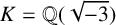 with the complex multiplication
$[\omega ]P$
 .
As a summary, we have the following proposition.
Proposition 3.4. Let us define

We set the degree of
$x, A', B'$
 as
$2, 4, 6$
 . Then we have the following:
-
(1) For $N = 2m+1$
with
$m \ge 1$
, we define Then, this is a polynomial in $\mathbb {Z} [x, A', B' ]$
, homogeneous of degree
$N^2-1$
. Moreover, as a polynomial of x, the leading coefficient is
$N = 2m+1$
.
-
(2) For $n = 2m+2$
with
$m \ge 1$
, Then, this is a polynomial in $\mathbb {Z} [x, A', B' ]$
, homogeneous of degree
$N^2-4$
. Moreover, as a polynomial in x, the leading coefficient is
$N/2 = m$
.



Using this proposition, we estimate the denominator of the minimal polynomial of
$f_a(\tau )$
 over
$\mathbb {Q}(j(\tau ))$
 .
4 Arithmetic smoothness
The results discussed above provide us a basis for the target algorithm to judge the integrality of algebraic Witt vectors
$\xi = F(\widehat {f}_a)$
 represented by polynomials
$F(z_a)$
 , which we outline in Section 4.1. First we give the algorithm separately in the case where K is of class number one, in particular; some necessary treatment for the general case algorithm is given afterwards. Needless to say, the general case algorithm works equally for the case of class number one as well, but in that special case, the operators
$\delta _{\mathfrak {p}}$
 are globally available. So the algorithm in the special case (that is, the case of class number one) is formulated explicitly using the operators
$\delta _{\mathfrak {p}}$
 ; the general case algorithm is built using a localization argument. After this outline of algorithms, we prove in Section 4.2 some facts on algebraic Witt vectors necessary for verification of these algorithms.
4.1 Outline of algorithm
4.1.1 The special case
The problem here is that, given
$\xi = F(\widehat {f}_a) \in E_K$
 , we need to judge whether
$\xi $
 belongs to
$A_K$
 , or in elementary words, we need to judge whether the components of the arithmetic derivatives
$\delta _{\mathfrak {p}_1} \delta _{\mathfrak {p}_2} \cdots \delta _{\mathfrak {p}_N} \xi $
 of
$\xi $
 are integers for all
$N \geq 0$
 and any
$\mathfrak {p}_1, \ldots , \mathfrak {p}_N \in P_K$
 ; apparently, this itself is a priori impossible to check within finite steps. Therefore, our challenge here is to reduce this infinitary problem to some finitary one.
This reduction can be divided into two steps. First, for each
$\xi \in E_K$
 , it is sufficient to consider the arithmetic derivatives
$\delta _{\mathfrak {p}}$
 only for finitely many
$\mathfrak {p} \in P_K$
 , depending on
$\xi $
 : As discussed in [Reference Uramoto15, Section 4.3], each
$\xi $
 belongs to a certain
$\Lambda $
 -ring
$X_{NO_K}$
 , which is, as a finite etale K-algebra, of the form
$X_{NO_K} = \prod _{\mathfrak {d} \mid NO_K} K_{NO_K / \mathfrak {d}}$
 , where
$K_{\mathfrak {f}}$
 denotes the ray class field of K with conductor
$\mathfrak {f} \in I_K$
 . Therefore, for those
$\mathfrak {p} \in P_K$
 coprime to
$NO_K$
 , the action of
$\psi _{\mathfrak {p}}$
 on
$X_{NO_K}$
 is equal to that of the Frobenius automorphism
$\sigma _{\mathfrak {p}} $
 on each component
$K_{NO_K / \mathfrak {d}}$
 of
$X_{NO_K}$
 , hence on
$\xi $
 as well. This implies that our problem for
$\xi \in X_{NO_K}$
 is reduced to considering the arithmetic derivatives
$\delta _{\mathfrak {p}}$
 only for those
$\mathfrak {p}$
 that divide
$NO_K$
 ; also
$N \in \mathbb {N}$
 can be chosen so that the indices
$a \in \mathbb {Q}^2/\mathbb {Z}^2$
 appearing in
$\xi = F(\widehat {f}_a)$
 are all in
$N^{-1}\mathbb {Z}^2/\mathbb {Z}^2$
 . Moreover, since
$X_{NO_K} = \mathrm {Hom}_{G_K}(DR_{NO_K}, \bar {K})$
 , all the components
$\xi _{\mathfrak {a}}$
 of
$\xi \in X_{NO_K}$
 are determined by those at
$\mathfrak {a}_1, \ldots , \mathfrak {a}_k$
 , which represent the elements of the finite ray class monoid
$DR_{NO_K} = \bigsqcup _{\mathfrak {d} \mid NO_K} [\mathfrak {d}] \cdot C_{NO_K / \mathfrak {d}}$
 , where
$C_{\mathfrak {f}}$
 denotes the ray class group of K with conductor
$\mathfrak {f} \in I_K$
 (see [Reference Uramoto15, Section 2.1]).
Nevertheless this first step only is not yet sufficient for our goal; in fact, even with finitely many
$\mathfrak {p} \mid NO_K$
 , we still need to judge whether
$\xi \in X_{NO_K}$
 is differentiable infinitely many times with respect to those finitely many
$\mathfrak {p} \mid NO_K$
 . The second step to reduce this is to show that
$\xi \in X_{NO_K}$
 is differentiable infinitely many times with respect to all
$\mathfrak {p} \mid NO_K$
 if and only if it is differentiable at least M times for some finite number M by those
$\mathfrak {p} \mid NO_K$
 , an upper bound of which is calculable for
$\xi \in X_{NO_K}$
 . We can show this fact based on the finiteness of the integral closure
$B_\xi $
 of
$O_K$
 in
$X_\xi $
 (see [Reference Uramoto15, Section 3.1]); to be more specific, we estimate the above
$M \in \mathbb {N}$
 for
$\xi $
 based on two facts on certain
$O_K$
 -algebras
$D_n$
 : Let us denote by
$D_n \subseteq X_\xi $
 for
$n \in \mathbb {N}$
 the
$O_K$
 -subalgebra of
$X_\xi $
 generated by r-times derivatives
$\delta _{\mathfrak {p}_{i_1}} \cdots \delta _{\mathfrak {p}_{i_r}} \xi $
 of
$\xi $
 with respect to
$\mathfrak {p}_{i_l} \mid NO_K$
 up to
$r \leq n$
 ; this gives rise to the ascending sequence
$D_0 \subseteq D_1 \subseteq \cdots \subseteq D_n \subseteq \cdots \subseteq X_\xi $
 of
$O_K$
 -subalgebras. Concerning this, note first that
$D_n$
 becomes full rank in
$X_\xi $
 (that is,
$K \otimes D_n = X_\xi $
 ) after some
$n_1$
 , which is explicitly calculable from our current N; this follows just from the facts that (i) for
$X_\xi = K[\psi _{\mathfrak {a}} \xi \mid \mathfrak {a} \in I_K]$
 , we can choose finitely many
$\mathfrak {a}$
 s from representatives of
$DR_{NO_K}$
 so that such finitely many
$\psi _{\mathfrak {a}} \xi $
 s already generate
$X_\xi $
 ; and (ii)
$\psi _{\mathfrak {p}} \xi = \xi ^{N\mathfrak {p}} + \pi _{\mathfrak {p}} \delta _{\mathfrak {p}} \xi $
 and conversely
$\delta _{\mathfrak {p}} \xi = \pi _{\mathfrak {p}}^{-1} (\psi _{\mathfrak {p}} \xi - \xi ^{N\mathfrak {p}})$
 by definition, hence
$\psi _{\mathfrak {p}} \xi $
 and
$\delta _{\mathfrak {p}} \xi $
 generate the same algebra over K together with
$\xi $
 . Therefore, for all
$n \geq n_1$
 , the
$O_K$
 -algebras
$D_n$
 are of full rank in
$X_\xi $
 . Note also that we have either (I) some n-times derivative of
$\xi $
 is judged as nonintegral by means of Section 3 at some
$n \geq n_1$
 , whence we conclude that
$\xi $
 is not integral; or (II) the ascending sequence of
$D_n$
 s terminates at some
$n_2 \geq n_1$
 because
$B_\xi $
 is finite over
$O_K$
 ; thus by construction, the quotient
$O_K$
 -module
$B_\xi / D_{n_1}$
 is of finite cardinarity. The point in the latter case (II) is that (i) such
$n_2$
 can be estimated from
$\xi $
 , and also (ii) if
$\xi $
 is at least
$n_2$
 -times differentiable for all
$\mathfrak {p} \mid NO_K$
 , it follows that
$\xi $
 is in fact differentiable infinitely many times (thanks to
$D_{n_2} = D_{n_2 + 1} = \cdots $
 ), whence we can conclude that
$\xi $
 is an integral Witt vector. (Thus, we can take
$M = n_2$
 .) On the whole, this procedure is finitary, which is what we need.
4.1.2 The general case
The basic idea for the general-case algorithm is almost the same as the special case. But in the general case, the operators
$\delta _{\mathfrak {p}}$
 are no longer (globally) available; so we need some additional treatment for the general case.
As briefly predicted in [Reference Ishitsuka and Uramoto9] too, the key is the good behavior of the Witt vector functor [Reference Borger1] with respect to the localization operations, from which we can deduce the following natural isomorphism of rings (see Section 4.2 for more precise details):

From this isomorphism, the problem of judging whether
$\xi \in W_{O_K}^a(O_{\bar {K}}) = A_K$
 is reduced to the local problems of judging whether
$\xi \in W_{O_{K, \mathfrak {p}}, P_K^{(\mathfrak {p})}} (O_{K, \mathfrak {p}} \otimes O_{\bar {K}})$
 for all
$\mathfrak {p}$
 ; then we can use the operators
$\delta _{\mathfrak {p}}$
 locally at each
$\mathfrak {p}$
 .
As in the special case, we need only to consider finitely many
$\mathfrak {p}$
 such that
$\mathfrak {p} \mid NO_K$
 if
$\xi \in X_{NO_K}$
 ; therefore, the remaining task is to judge local smoothness of
$\xi $
 , namely,
${\xi \in W_{O_{K, \mathfrak {p}}, P_K^{(\mathfrak {p})}} (O_{K, \mathfrak {p}} \otimes O_{\bar {K}})}$
 using the local (and thus single) derivative
$\delta _{\mathfrak {p}}$
 for each
${\mathfrak {p} \mid NO_K}$
 . The first major difference from the special case is that, at each step of derivation, we need to judge whether the coefficients of the derivatives
$\delta _{\mathfrak {p}}^r \xi $
 are all in the localized ring
$O_{K, \mathfrak {p}} \otimes O_{\bar {K}}$
 rather than
$O_{\bar {K}}$
 ; hence, they do not need to be integers globally and may have nontrivial denominators in
$O_K \setminus \mathfrak {p}$
 , which makes our decision problem slightly more delicate.
To be specific, we need to check whether the coefficients
$(\delta _{\mathfrak {p}}^r \xi )_{\mathfrak {a}} \in \bar {K}$
 of
$\delta _{\mathfrak {p}}^r \xi $
 are all in
$O_{K, \mathfrak {p}} \otimes O_{\bar {K}}$
 , that is, whether
$b \cdot (\delta _{\mathfrak {p}}^r \xi )_{\mathfrak {a}} \in O_{\bar {K}}$
 for
$\exists\ b \in O_K \setminus \mathfrak {p}$
 ; the existential quantifier
$\exists $
 here is a new obstruction to our decision procedure. However, since we can now estimate the denominators of the coefficients of
$\delta _{\mathfrak {p}}^r \xi $
 thanks to Section 3, the possible denominators of the coefficients of
$\delta _{\mathfrak {p}}^r \xi $
 in
$O_K \setminus \mathfrak {p}$
 can be bounded, which implies that we in fact need only to consider finitely many possible denominators from
$O_K \setminus \mathfrak {p}$
 (see Section 4.2).
The second major difference from the special case is that, in the general case, we need to consider the
$O_{K,\mathfrak {p}}$
 -subalgebras (instead of
$O_K$
 -subalgebras)
$D^{(\mathfrak {p})}_n$
 of the K-algebra
$X_\xi $
 generated over
$O_{K, \mathfrak {p}}$
 by the derivatives
$\delta _{\mathfrak {p}}^r \xi $
 for
$r \leq n$
 . As in the special case, this gives rise to the ascending sequence
$D_0^{(\mathfrak {p})} \subseteq D_1^{(\mathfrak {p})} \subseteq \cdots \subseteq D_n^{(\mathfrak {p})} \subseteq \cdots \subseteq X_\xi $
 of
$O_{K, \mathfrak {p}}$
 -subalgebras of
$X_\xi $
 ; however, unlike the special case, the corresponding K-algebras
$K \otimes D_0^{(\mathfrak {p})} \subseteq K \otimes D_1^{(\mathfrak {p})} \subseteq \cdots \subseteq K \otimes D_n^{(\mathfrak {p})} \subseteq \cdots \subseteq X_\xi $
 do not necessarily converge to
$X_\xi $
 . Nevertheless, we can estimate when the K-algebra
$K \otimes D_n^{(\mathfrak {p})}$
 terminates, or in other words, when
$D_n^{(\mathfrak {p})}$
 becomes full rank in
$\lim _n K \otimes D_n^{(\mathfrak {p})}$
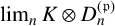 . Denoting
$X_{\xi }^{(\mathfrak {p})} := \lim _n K \otimes D_n^{(\mathfrak {p})} = K \otimes D_{n_1}$
 for some
$n_1 \geq 0$
 , this K-algebra
$X_{\xi }^{(\mathfrak {p})}$
 is finite etale over K; thus the integral closure
$B_\xi ^{(\mathfrak {p})}$
 of
$O_{K, \mathfrak {p}}$
 within
$X_\xi ^{(\mathfrak {p})}$
 is finite over
$O_{K, \mathfrak {p}}$
 . Again, as in the special case, the quotient
$O_{K, \mathfrak {p}}$
 -module
$B_\xi ^{(\mathfrak {p})} / D_{n_1}^{(\mathfrak {p})}$
 is of finite cardinality, the size of which can be estimated from
$\xi $
 by elementary module-theoretic arguments; from this estimate, we can then bound
$n_2 \geq n_1$
 , whence
$D_n^{(\mathfrak {p})}$
 terminates. Based on these facts, it follows that
$\xi $
 is locally smooth (that is,
$\xi \in W_{O_{K, \mathfrak {p}}, P_K^{(\mathfrak {p})}} (O_{K, \mathfrak {p}} \otimes O_{\bar {K}})$
 ) if and only if it is locally differentiable at least
$n_2$
 -times by
$\mathfrak {p}$
 (thanks to
$D_{n_2}^{(\mathfrak {p})} = D_{n_2 + 1}^{(\mathfrak {p})} = \cdots $
 ). This can be checked within finite steps thanks to the above (first) argument concerning denominators in
$O_K \setminus \mathfrak {p}$
 ; on the whole, this is finitary and we are done.
4.2 Proof of the algorithm
Here we prove nontrivial claims appearing in the above outline of our algorithms. To this end, we first recall the structure of the K-algebra
$X_\xi = K [\psi _{\mathfrak {a}} \xi \mid \mathfrak {a} \in I_K]$
 generated over K by the orbit
$I_K \xi $
 of
$\xi $
 under the action of
$\psi _{\mathfrak {p}}$
 s; in particular, it is essential for our algorithm that this K-algebra
$X_\xi $
 is finite etale over K [Reference Uramoto13, Proposition 4]. To be more specific, the K-algebra
$X_\xi $
 has the following presentation given in terms of components
$\xi _{\mathfrak {a}}$
 of
$\xi $
 .
Proposition 4.1 (see [Reference Uramoto15, Proposition 3.2.5]).
For
$\xi \in E_K$
 , we have the following isomorphism as a finite etale K-algebra:

Here
$M_\xi $
 is the finite monoid defined as the quotient monoid
$I_K / \equiv _\xi $
 , where
$\mathfrak {a} \equiv _\xi \mathfrak {b}$
 for
$\mathfrak {a}, \mathfrak {b} \in I_K$
 if and only if
$\psi _{\mathfrak {a}} \xi = \psi _{\mathfrak {b}} \xi $
 ; and
$\mathcal {J}$
 is Green’s
$\mathcal {J}$
 -equivalence relation on the finite monoid
$M_\xi $
 , that is,
$[\mathfrak {a}] \mathcal {J} [\mathfrak {b}]$
 for
$[\mathfrak {a}], [\mathfrak {b}] \in M_\xi $
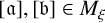 if and only if
$[\mathfrak {a} \mathfrak {c}] = [\mathfrak {b}]$
 and
$[\mathfrak {b} \mathfrak {d}] = [\mathfrak {a}]$
 for some
$[\mathfrak {c}], [\mathfrak {d}] \in M_\xi $
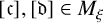 ; in other words, this is precisely when
$[\mathfrak {a}]$
 and
$[\mathfrak {b}]$
 generate the same two-sided ideal in
$M_\xi $
 . We abusively denote by
$[\mathfrak {a}]$
 (or by
$[\mathfrak {a}]_{\mathcal {J}}$
 ) the
$\mathcal {J}$
 -equivalence class for
$[\mathfrak {a}] \in M_\xi $
 . It is shown in [Reference Uramoto15, Lemma 3.2.4] that
$[\mathfrak {a}] \in M_\xi $
 and
$[\mathfrak {b}] \in M_\xi $
 are
$\mathcal {J}$
 -equivalent if and only if
$[\mathfrak {a}] \cdot M_\xi ^\times = [\mathfrak {b}] \cdot M_\xi ^\times $
 , where
$M_\xi ^\times $
 denotes the unit group of
$M_\xi $
 . Choosing complete representatives
$[\mathfrak {a}_1]_{\mathcal {J}}, \ldots , [\mathfrak {a}_n]_{\mathcal {J}}$
 of
$M_\xi / \mathcal {J}$
 , the above isomorphism of
$X_\xi $
 is given as follows (see [Reference Uramoto15, Proposition 3.2.5]):

Here it is useful to recognize a more concise presentation of each component
${K(\xi _{\mathfrak {a}_i \mathfrak {b}} \mid \mathfrak {b} \in I_K)}$
 of the right-hand side. For this, in relation to the above
$\mathcal {J}$
 -equivalence on
$M_\xi $
 , we define a quasiordering
$\leq _{\mathcal {J}}$
 on
$M_\xi $
 : that is,
$[\mathfrak {a}] \leq _{\mathcal {J}} [\mathfrak {b}]$
 for
$[\mathfrak {a}], [\mathfrak {b}] \in M_\xi $
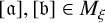 if and only if
$[\mathfrak {a}] = [\mathfrak {b} \mathfrak {c}]$
 for some
$[\mathfrak {c}] \in M_\xi $
 ; thus, by definition,
$[\mathfrak {a}] \mathcal {J} [\mathfrak {b}]$
 if and only if
$[\mathfrak {a}] \leq _{\mathcal {J}} [\mathfrak {b}]$
 and
$[\mathfrak {a}] \geq _{\mathcal {J}} [\mathfrak {b}]$
 . With this notation, notice first that if
$[\mathfrak {a}] = [\mathfrak {b}]$
 we have
$\psi _{\mathfrak {a}} \xi = \psi _{\mathfrak {b}} \xi $
 by definition, hence, in particular,
$\xi _{\mathfrak {a}} = \xi _{\mathfrak {b}}$
 . Therefore, it makes sense to denote
$\xi _{[\mathfrak {a}]} := \xi _{\mathfrak {a}}$
 ; the same is true for every
$\eta \in X_\xi $
 . With the above representatives
$[\mathfrak {a}_1]_{\mathcal {J}}, \ldots , [\mathfrak {a}_n]_{\mathcal {J}}$
 of
$M_\xi / \mathcal {J}$
 , the component
$K(\xi _{\mathfrak {a}_i \mathfrak {b}} \mid \mathfrak {b} \in I_K)$
 is then equal to
$K(\xi _{[\mathfrak {b}]} \mid [\mathfrak {b}] \leq _{\mathcal {J}} [\mathfrak {a}_i])$
 , hence,

Furthermore, the K-algebra
$X_\xi $
 is equipped with the
$\Lambda $
 -structure
$\psi _{\mathfrak {p}}: X_\xi \rightarrow X_\xi $
 for each
$\mathfrak {p} \in I_K$
 , which admits a simple description. That is, for each
$\eta \in X_\xi $
 and
$\mathfrak {p} \in I_K$
 ,
$\psi _{\mathfrak {p}} \eta \in X_\xi $
 corresponds to
$(\eta _{[\mathfrak {p} \mathfrak {a}_1]}, \ldots , \eta _{[\mathfrak {p} \mathfrak {a}_n]})$
 under the above isomorphism.
From a computational standpoint, we need to further concsider how to compute (the multiplication table of) the finite monoid
$M_\xi $
 and how to effectively choose representatives of
$M_\xi $
 and
$M_\xi / \mathcal {J}$
 ; in fact, the finite monoid
$M_\xi $
 is defined as the quotient monoid
$I_K / \equiv _\xi $
 , but to judge the equivalence relation
$\mathfrak {a} \equiv _\xi \mathfrak {b}$
 , we need to judge the equality
$\psi _{\mathfrak {a}} \xi = \psi _{\mathfrak {b}} \xi $
 , namely
$\xi _{\mathfrak {a} \mathfrak {c}} = \xi _{\mathfrak {b} \mathfrak {c}}$
 for all
$\mathfrak {c} \in I_K$
 . This seemingly infinitary problem, however, can be reduced to a finitary problem, thanks to the fact that
$M_\xi $
 is a quotient of
$DR_{NO_K}$
 if the indices
$a \in \mathbb {Q}^2 / \mathbb {Z}^2$
 appearing in
$\xi = F(\widehat {f}_a)$
 are all in
$N^{-1} \mathbb {Z}^2 / \mathbb {Z}^2$
 , which gives a kind of upper bound for our search.
Proposition 4.2. There is an effective procedure to construct the multiplication table of
$M_\xi $
 and to choose representatives of
$M_\xi $
 and
$M_\xi / \mathcal {J}$
 .
Proof. We can list representatives of
$DR_{NO_K} = \coprod _{\mathfrak {d} \mid NO_K} [ \mathfrak {d} ] \cdot C_{NO_K / \mathfrak {d}}$
 ; therefore, we need only to consider such representatives in the construction of
$M_\xi $
 as well. This means that we need to consider only finitely many coefficients
$\xi _{\mathfrak {a}}$
 at those
$\mathfrak {a}$
 that represent
$DR_{NO_K}$
 . Thus, we can also judge the equality
$\psi _{\mathfrak {a}} \xi = \psi _{\mathfrak {b}} \xi $
 , hence the equivalence
$\mathfrak {a} \equiv _\xi \mathfrak {b}$
 . (Note that, by the estimate of denominators in Section 3, we can decide whether two special values of Fricke functions are equal.)
Definition 4.3 (conductor of
$\xi $
).

For
$\xi \in E_K$
 , the conductor
$\mathfrak {f}_\xi \in I_K$
 of
$\xi $
 is defined so that, for each
$\mathfrak {p} \in P_K$
 :

We start from the special case; for a while, assume that K is of class number one, whence
$O_K$
 is a PID. The following says that, to judge the arithmetic smoothness of
$\xi $
 , we actually need to consider arithmetic derivatives
$\delta _{\mathfrak {p}}$
 for only finitely many
$\mathfrak {p}$
 s.
Lemma 4.4. Let
$\mathfrak {f}_\xi \in I_K$
 be the conductor of
$\xi \in E_K$
 . Then
$\xi $
 is arithmetically smooth, namely
$\xi \in A_K$
 if and only if
$\delta _{\mathfrak {p}_{i_1}} \cdots \delta _{\mathfrak {p}_{i_N}} \xi \subseteq O_{\bar {K}}^{I_K}$
 for any
$N \geq 0$
 and any
$\mathfrak {p}_i \mid \mathfrak {f}_\xi $
 .
Proof. The only-if part is trivial; so we prove the if part. But this follows from the fact that, for
$\mathfrak {p} \in P_K$
 coprime to
$\mathfrak {f}_\xi $
 , the action of
$\psi _{\mathfrak {p}}$
 on
$X_\xi $
 is an automorphism, thus equal to the component-wise action of the Frobenius automorphism
$\sigma _{\mathfrak {p}}$
 (see [Reference Uramoto15, Lemma 3.2.1]) on
$X_\xi $
 .
Remark 4.5. If
$\xi \in X_{NO_K}$
 , we have
$\mathfrak {f}_\xi \mid NO_K$
 .
Definition 4.6. Fix
$\xi \in E_K$
 ; we define
$D_n$
 to be the
$O_K$
 -subalgebra of
$X_\xi $
 generated by r-times derivatives
$\delta _{\mathfrak {p}_{i_1}} \cdots \delta _{\mathfrak {p}_{i_r}} \xi $
 of
$\xi $
 with respect to
$\mathfrak {p}_i \mid \mathfrak {f}_\xi $
 up to
$r \leq n$
 .
Lemma 4.7. Let
$\mathfrak {f}_\xi $
 be the conductor of
$\xi \in E_K$
 exactly with the prime factors
$\mathfrak {p}_1, \ldots , \mathfrak {p}_m$
 ; and put
$n_1 := \sum _{i=1}^m v_{\mathfrak {p}_i}(\mathfrak {f}_\xi )$
 . Then
$D_{n_1}$
 is of full rank in
$X_\xi $
 .
Proof. Let
$X_n$
 be the K-subalgebra of
$X_\xi $
 generated by
$\psi _{\mathfrak {a}} \xi $
 ’s for
$\mathfrak {a} \in I_K$
 of the form
$\mathfrak {a} = \mathfrak {p}_1^{e_1} \cdots \mathfrak {p}_m^{e_m}$
 with
$\sum _i e_i \leq n_1$
 . Firstly, by induction on n, we can see that
$X_n = K \otimes D_n$
 by the general fact that
$\delta _{\mathfrak {p}} \eta $
 and
$\psi _{\mathfrak {p}} \eta $
 generate the same algebra over K together with
$\eta $
 . Therefore, it suffices to show that
$X_{n_1} = X_\xi $
 . By definition, note that
$\psi _{\mathfrak {a}} \xi $
 s for
$\mathfrak {a} \in I_K$
 of the form
$\mathfrak {a} = \mathfrak {p}_1^{e_1} \cdots \mathfrak {p}_m^{e_m}$
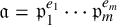 with
$\sum _i e_i \leq n_1$
 and their Galois conjugates generate
$X_\xi $
 ; but note also that
$X_{n_1}$
 is closed under the action of
$G_K^{ab}$
 . Thus, we have
$X_{n_1} = X_\xi $
 .
If
$D_{n_1}$
 already contains a nonintegral Witt vector, then we can conclude that
$\xi $
 is not integral; otherwise, we need to continue to check whether the arithmetic derivatives
$\delta _{\mathfrak {p}_1} \cdots \delta _{\mathfrak {p}_n} \xi $
 of
$\xi $
 have integral components for all
$n \geq n_1$
 . This task itself is an infinitely problem, especially when
$\xi $
 is an integral Witt vector; but by the following key estimate, we can actually stop this procedure at some finitely many times.
Lemma 4.8. Suppose that
$\xi $
 is an integral Witt vector; let
$n_1$
 be as above. Then we can effectively estimate an upper bound of
$n \geq n_1$
 when
$D_n$
 terminates.
Proof. We first construct a K-basis of
$X_\xi $
 . To this end, it suffices to find K-bases of the components
$L_i:= K(\xi _{[\mathfrak {b}]} \mid [\mathfrak {b}] \leq _{\mathcal {J}} [\mathfrak {a}_i])$
 by
$X_\xi = \prod _i K(\xi _{[\mathfrak {b}]} \mid [\mathfrak {b}] \leq _{\mathcal {J}} [\mathfrak {a}_i])$
 ; here note that
$\dim _K K(\xi _{[\mathfrak {b}]} \mid [\mathfrak {b}] \leq _{\mathcal {J}} [\mathfrak {a}_i]) = \# ( [\mathfrak {a}_i] \cdot M_\xi ^\times ) =: n_i$
 . In particular, since each
$L_i$
 is Galois over K, we can effectively construct an algebraic integer
$c_i$
 such that
$L_i = K(c_i)$
 from the generators
$\xi _{[\mathfrak {b}]}$
 , for example, by the method of Steinitz’ theorem (see, for example, [Reference Rotman10, Theorem 86]), so that
$1, c_i, c_i^{2}, \ldots , c_i^{n_i-1}$
 give a K-basis of
$L_i$
 .
Let
$D_i$
 be the discriminant of
$1, c_i, \ldots , c_i^{n_i -1}$
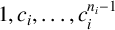 over K, so that the free
$O_K$
 -module
${B_i := O_K \oplus O_K \cdot (c_i/D_i) \oplus \cdots \oplus O_K \cdot (c_i^{n_i -1}/D_i)}$
 contains the integer ring
$O_{L_i}$
 of
$L_i$
 . Then, the product
$O_K$
 -submodule
$\prod B_i \subset X_\xi $
 contains the integral closure
$\prod _i O_{L_i}$
 of
$O_K$
 within
$X_\xi $
 and hence
$D_{n_1}$
 too by assumption; with respect to the
$O_K$
 -basis of
$B = \prod B_i$
 obtained from
$c_i^k/D_i$
 ’s, we then represent an
$O_K$
 -basis of
$D_{n_1}$
 as an
$O_K$
 -coefficient matrix C. (Note that since we know by construction finitely many
$O_K$
 -linear generators of
$D_{n_1}$
 , we can also choose an
$O_K$
 -basis from them effectively.) Let N be the absolute norm of the determinant of the matrix C; the size
$|B/D_{n_1}|$
 of the finite
$O_K$
 -module
$B/D_{n_1}$
 is not greater than N. Therefore, the ascending chain
$D_{n_1} \subseteq D_{n_1 + 1} \subseteq \cdots \subseteq D_n$
 terminates within B at latest
$n_2 = n_1 + 2^N$
 , hence the claim follows.
Theorem 4.9. Let
$\mathfrak {f}_\xi $
 be the conductor of
$\xi \in E_K$
 and
$n_2$
 be as above. Then
$\xi \in E_K$
 belongs in
$A_K$
 if and only if
$\xi $
 is at least
$n_2$
 -times differentiable with
$\mathfrak {p} \mid \mathfrak {f}_\xi $
 .
Proof. If
$\xi $
 is not integral, some derivative of
$\xi $
 is judged as nonintegral by means of Section 3. Otherwise, by definition of
$n_2$
 , we have
$D_{n_2} = D_{n_2 + 1} = \cdots = D_n = \cdots $
 for all
$n \geq n_2$
 ; therefore, if the at most
$n_2$
 -times arithmetic derivatives of
$\xi $
 all have integral components, then we can conclude that
$\xi $
 is an integral Witt vector, hence the claim follows.
We now consider the general case; a key for this is the following.
Lemma 4.10. For
$\xi \in E_K$
 , we have the following equivalence:

Proof. To see this we note the following isomorphism:

To be precise, we first have the identity
$W_{O_K}(O_{\bar {K}}) = \bigcap _{\mathfrak {p}} O_{K, \mathfrak {p}} \otimes W_{O_K} (O_{\bar {K}})$
 ; then by Proposition 6.1 and by (2.4.2) [Reference Borger1], we have a canonical isomorphism
$O_{K, \mathfrak {p}} \otimes W_{O_K}(O_{\bar {K}}) \simeq W_{O_{K, \mathfrak {p}}, P_K^{(\mathfrak {p})}} (O_{K, \mathfrak {p}} \otimes O_{\bar {K}})$
 . Here
$P_K^{(\mathfrak {p})}$
 denotes the set of ideals
$\mathfrak {m}_{\mathfrak {q}} \subseteq O_{K, \mathfrak {p}}$
 indexed by
$\mathfrak {q} \in P_K$
 such that
$\mathfrak {m}_{\mathfrak {p}} = \mathfrak {p} O_{K, \mathfrak {p}}$
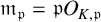 and
$\mathfrak {m}_{\mathfrak {q}} = O_{K, \mathfrak {p}}$
 for
$\mathfrak {q} \neq \mathfrak {p}$
 , hence the claim follows.
Lemma 4.11. Let
$\pi _{\mathfrak {p}} \in \mathfrak {p}$
 be a uniformizer of
$\mathfrak {p}$
 ; and define
$\delta _{\mathfrak {p}} \eta := \pi _{\mathfrak {p}}^{-1} (\psi _{\mathfrak {p}} \eta - \eta ^{N\mathfrak {p}})$
 . With this notation, we have the following equivalence for
$\xi \in E_K$
 :

Proof. By definition (see [Reference Borger1]),
$\xi \in W_{O_{K, \mathfrak {p}}, P_K^{(\mathfrak {p})}} (O_{K, \mathfrak {p}} \otimes O_{\bar {K}})$
 if and only if
$\xi $
 is infinitely differentiable by all
$\mathfrak {m}_{\mathfrak {q}} \in P_K^{(\mathfrak {p})}$
 . But recall that
$\mathfrak {m}_{\mathfrak {q}} = O_{K, \mathfrak {p}}$
 for all
$\mathfrak {q} \neq \mathfrak {p}$
 , hence the arithmetic smoothness with respect to
$\mathfrak {m}_{\mathfrak {q}}$
 for
$\mathfrak {q} \neq \mathfrak {p}$
 is trivial. Therefore, the arithmetic smoothness with respect to
$\mathfrak {m}_{\mathfrak {p}}$
 only matters.
Thanks to the above lemmas, our target decision problem
$\xi \in W_{O_K}^a(O_{\bar {K}})$
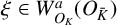 is now reduced to the local problems
$\xi \in W_{O_{K, \mathfrak {p}}, P_K^{(\mathfrak {p})}} (O_{K, \mathfrak {p}} \otimes O_{\bar {K}})$
 at
$\mathfrak {p} \mid \mathfrak {f}_\xi $
 ; but instead, we then need to be able to judge whether the coefficients of the derivatives
$\delta _{\mathfrak {p}}^r \xi $
 of
$\xi $
 is in the localized ring
$O_{K, \mathfrak {p}} \otimes O_{\bar {K}}$
 rather than
$O_{\bar {K}}$
 . The following lemma provides what we need for this task.
Lemma 4.12. Let
$\mathfrak {p} \in P_K$
 and
$\alpha \in \bar {K}$
 such that
$N \cdot \alpha \in O_{\bar {K}}$
 for some rational integer N. Then we can decide whether
$\alpha \in O_{K, \mathfrak {p}} \otimes O_{\bar {K}}$
 .
Proof. If
$\mathfrak {p}$
 is coprime to
$NO_K$
 , then
$N \in O_K \setminus \mathfrak {p}$
 ; thus
$\alpha \in O_{K, \mathfrak {p}} \otimes O_{\bar {K}}$
 . Otherwise (that is,
$\mathfrak {p} \mid NO_K$
 ), let
$O_K / N O_K = \{b_1, \ldots , b_m\}$
 . By definition,
$\alpha \in O_{K, \mathfrak {p}} \otimes O_{\bar {K}}$
 if and only if there exists some
$b \in O_K \setminus \mathfrak {p}$
 such that
$b \cdot \alpha \in O_{\bar {K}}$
 ; but the latter condition is now equivalent to the fact that there exists some i such that
$b_i \cdot \alpha \in O_{\bar {K}}$
 and
$b_i \in O_K \setminus \mathfrak {p}$
 , which is hence decidable.
Definition 4.13. Fix
$\xi \in E_K$
 and
$\mathfrak {p} \in P_K$
 ; let us define
$D_n^{(\mathfrak {p})}$
 to be the
$O_{K, \mathfrak {p}}$
 -subalgebra of
$X_\xi $
 generated by the r-times derivatives
$\delta _{\mathfrak {p}}^r \xi $
 of
$\xi $
 up to
$r \leq n$
 .
The next task is to estimate when the ascending sequence
$K \otimes D_0^{(\mathfrak {p})} \subseteq K \otimes D_1^{(\mathfrak {p})} \subseteq \cdots \subseteq X_\xi $
 of K-subalgebras of
$X_\xi $
 terminates; we denote by
$X_\xi ^{(\mathfrak {p})} = \lim _n K \otimes D_n^{(\mathfrak {p})}$
 the limit K-algebra.
Lemma 4.14. Let
$\mathfrak {f}_\xi \in I_K$
 be the conductor of
$\xi \in E_K$
 and
$n_1 := v_{\mathfrak {p}} (\mathfrak {f}_\xi )$
 . Then the ascending sequence
$K \otimes D_0^{(\mathfrak {p})} \subseteq K \otimes D_1^{(\mathfrak {p})} \subseteq \cdots \subseteq X_\xi $
 of K-subalgebras terminates at
$n_1$
 .
Proof. By definition of
$n_1$
 , the action of
$\psi _{\mathfrak {p}}$
 on
$\psi _{\mathfrak {p}}^{n_1} X_\xi $
 becomes an automorphism; hence we have the identity
$K[\psi _{\mathfrak {p}}^r \xi \mid r \leq n_1] = K[\psi _{\mathfrak {p}}^r \xi \mid r \geq 0]$
 . Note that the former K-algebra is equal to
$K \otimes D_{n_1}$
 by the fact that
$\psi _{\mathfrak {p}} \eta $
 and
$\delta _{\mathfrak {p}} \eta $
 generate the same K-algebra together with
$\eta $
 , hence the claim follows.
Lemma 4.15. Suppose that
$\xi $
 belongs in
$W_{O_{K, \mathfrak {p}}, P_K^{(\mathfrak {p})}} (O_{K, \mathfrak {p}} \otimes O_{\bar {K}})$
 . Then we can estimate an upper bound of
$n_2$
 whence the ascending sequence
$D_0^{(\mathfrak {p})} \subseteq D_1^{(\mathfrak {p})} \subseteq \cdots \subseteq D_n^{(\mathfrak {p})} \subseteq \cdots $
 of
$O_{K,\mathfrak {p}}$
 -subalgebras of
$X_\xi ^{(\mathfrak {p})}$
 terminates.
Proof. By the method of Lemma 4.8, take a K-basis
$\{\eta _1^{(\mathfrak {p})}, \ldots , \eta _m^{(\mathfrak {p})} \}$
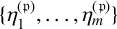 of
$X_\xi ^{(\mathfrak {p})}$
 such that the
$O_{K,\mathfrak {p}}$
 -module
$O_{K,\mathfrak {p}} \eta _1^{(\mathfrak {p})} \oplus \cdots \oplus O_{K,\mathfrak {p}} \eta _m^{(\mathfrak {p})}$
 contains the integral closure of
$O_{K,\mathfrak {p}}$
 within
$X_\xi ^{(\mathfrak {p})}$
 , hence it contains
$D_{n_1}$
 as well by the assumption; here we denote it as
$B^{(\mathfrak {p})}$
 . Then the quotient
$O_{K,\mathfrak {p}}$
 -module
$B^{(\mathfrak {p})} / D_{n_1}^{(\mathfrak {p})}$
 is of finite cardinality. To estimate its size, again as in Lemma 4.8, represent an
$O_{K, \mathfrak {p}}$
 -basis of
$D_{n_1}^{(\mathfrak {p})}$
 as an
$O_{K, \mathfrak {p}}$
 -coefficient matrix
$C^{(\mathfrak {p})}$
 with respect to the
$O_{K, \mathfrak {p}}$
 -basis
$\eta _1^{(\mathfrak {p})}, \ldots , \eta _m^{(\mathfrak {p})}$
 of
$B^{(\mathfrak {p})}$
 ; and let
$e \geq 0$
 be such that the ideal of
$O_{K, \mathfrak {p}}$
 generated by the determinant of
$C^{(\mathfrak {p})}$
 is equal to
$\mathfrak {p}^{e} O_{K, \mathfrak {p}}$
 ; then the size of
$B^{(\mathfrak {p})}/D_{n_1}^{(\mathfrak {p})}$
 is not greater than the absolute norm
$N:= N(\mathfrak {p}^e)$
 of
$\mathfrak {p}^e$
 . With this N, the ascending sequence
$D_0^{(\mathfrak {p})} \subseteq D_1^{(\mathfrak {p})} \subseteq \cdots \subseteq D_n^{(\mathfrak {p})} \subseteq \cdots $
 terminates at latest at
$n_2 = n_1 + 2^N$
 . This completes the proof.
Theorem 4.16. Let
$\mathfrak {f}_\xi $
 be the conductor of
$\xi \in E_K$
 . Then
$\xi \in E_K$
 belongs in
$A_K$
 if and only if for each
$\mathfrak {p} \mid \mathfrak {f}_\xi $
 with
$n_2$
 as above,
$\xi $
 is locally at least
$n_2$
 -times differentiable.
5 Concluding remarks
This paper proved that the integrality of algebraic Witt vectors over imaginary quadratic fields is decidable. Although we do not yet have a satisfactory description of the ring
$W_{O_K}^a(O_{\bar {K}})$
 of integral Witt vectors for number fields
$K \neq \mathbb {Q}$
 , this decidability enables us to construct and enumerate all integral Witt vectors
$\xi \in W_{O_K}^a(O_{\bar {K}})$
 for imaginary quadratic fields K. This improves our current understanding of the integral Witt vectors in view of the fact that we did not have even nontrivial examples of integral Witt vectors (other than the one given by the j-function, [Reference Uramoto15, Example 4.1.10]) for imaginary quadratic fields and any other number fields
$\neq \mathbb {Q}$
 .
We conclude this paper with the remark that the decidability of integral Witt vectors implies also that the maximal integral models of all galois objects of the semi-galois category
$\mathscr {C}_K$
 of Borger and de Smit [Reference Borger and de Smit3, Reference Borger and de Smit4] over imaginary quadratic fields can be effectively constructed. We need not recall the general definition of galois objects (see [Reference Uramoto14, Section 3]), as the galois objects of
$\mathscr {C}_K$
 are (up to isomorphism) precisely those of the form
$X_\Xi $
 for some finite
$\Xi \subseteq E_K$
 (see [Reference Uramoto15, Proposition 3.1.3]); this means that it is sufficient here to prove that we can construct the maximal integral model of
$X_\Xi $
 for any finite
$\Xi \subseteq E_K$
 .
Recall that, generally by an integral model of
$X_\Xi $
 , we mean a
$\Lambda $
 -subring
$A \subseteq X_\Xi $
 finite over
$O_K$
 such that
$X_\Xi = K\otimes A$
 as
$\Lambda $
 -rings over K; and by the maximal integral model, we mean an integral model, which contains every integral
$\xi \in X_\Xi $
 , that is, is maximal among integral models of
$X_\Xi $
 , hence the name. By this definition, the maximal integral model A of
$X_\Xi $
 is included in the integral closure
$B_\Xi $
 of
$O_K$
 within
$X_\Xi $
 ; thus to construct the maximal integral model, the same idea as those in Section 4 can be applied. Indeed, if we do not care about the computational efficiency, we can construct the maximal integral model of
$X_\Xi $
 by the following procedure, which one easily sees is effective:
-
(1) take a K-basis $\{\eta _1, \ldots , \eta _n\}$
of
$X_\Xi $
; -
(2) multiply a positive integer N by the $\eta _i$
s so that every
$\zeta _i := N \eta _i$
is integral; -
(3) construct an $O_K$
-module B that contains
$B_\Xi $
(as in Lemma 4.8); -
(4) find complete representatives $\xi _1, \ldots , \xi _m \in B$
of this
$B/ (O_K \zeta _1 + \cdots + O_K \zeta _n)$
; -
(5) find the integral ones $\{\xi _{i_1}, \ldots , \xi _{i_r}\}$
among the representatives
$\{\xi _1, \ldots , \xi _m\}$
; -
(6) the maximal integral model is given as $O_K \zeta _1 + \cdots + O_K \zeta _n + O_K \xi _{i_1} + \cdots + O_K \xi _{i_r}$
.






In this procedure, the decidability of integral Witt vectors is used in the second and fifth steps.
When one seeks a description of the ring
$W_{O_K}^a(O_{\bar {K}})$
 of integral Witt vectors, it would be helpful to recall the case of the rational number field
$\mathbb {Q}$
 . In this base case, the ring of integral Witt vectors is
$\mathbb {Z}[\widehat {e}_a \mid a \in \mathbb {Q}/\mathbb {Z}]$
 (Section 1), which is isomorphic to the group ring
$\mathbb {Z}[\mathbb {Q}/\mathbb {Z}]$
 (see [Reference Uramoto15, Corollary 3.3.1]); this was proved using the fact [Reference Borger and de Smit3] that the maximal integral model of the
$\Lambda $
 -ring
$\mathbb {Q}[x]/(x^N-1) \in \mathscr {C}_{\mathbb {Q}}$
 is
$\mathbb {Z}[x]/(x^N -1)$
 ; in terms of the galois objects of
$\mathscr {C}_{\mathbb {Q}}$
 , the
$\Lambda $
 -ring
$\mathbb {Q}[x]/(x^N - 1) \in \mathscr {C}_{\mathbb {Q}}$
 is the galois object corresponding to the conductor
$N\mathbb {Z} \in I_{\mathbb {Q}}$
 (see [Reference Uramoto15, Section 4.3]). To extend this explicit description of the maximal integral models
$\mathbb {Z}[x]/(x^N -1)$
 of
$\mathbb {Q}[x]/(x^N - 1)$
 to the case when K is an imaginary quadratic field, one should consult [Reference Borger and de Smit5, Theorem 11.12] of Borger and de Smit too; but as remarked in Related works, this theorem itself is not completely explicit nor K-intrinsic, compared to the case of
$\mathbb {Q}$
 . To obtain some more explicit description, our algorithm to construct integral Witt vectors and maximal integral models might be useful.
Acknowledgement
This work is an extended version of our short paper [Reference Ishitsuka and Uramoto9] announced at SCSS’21. We are grateful to Yoshihiro Mizoguchi for introducing us to SCSS’21; to the anonymous reviewer of SCSS’21 for his/her careful reading on [Reference Ishitsuka and Uramoto9]; and to Iwao Kimura for his advice on computational implementations. We are also grateful to the anonymous reviewer for his/her kind comments, corrections and suggestions, which improved this paper.



