2 The hydro-elastic system

We consider irrotational motion of an inviscid and incompressible fluid of undisturbed mean depth $H$ , and with gravity $g$ acting in the negative $z$ -direction. The fluid is covered by an elastic solid layer which is described by the Kirchhoff–Love plate theory (cf. Squire et al. Reference Squire, Hosking, Kerr and Langhorne1988b ). For the sake of readability, we first treat the two-dimensional problem, and return to the three-dimensional setting in § 5. The flow of the underlying liquid is described by the velocity potential $\unicode[STIX]{x1D719}(x,z,t)$ and by the fluid surface elevation $\unicode[STIX]{x1D702}(x,t)$ that coincides with the vertical deformation of the underside of the elastic cover. The fluid domain is the set $\{(x,z)\in \mathbb{R}^{2}\mid -H<z<\unicode[STIX]{x1D702}(x,t)\}$ extending to infinity in the positive and negative horizontal $x$ direction. The level $z=0$ corresponds to the fluid–solid interface at rest.

As explained for example in Whitham (Reference Whitham1974), the fluid flow is governed by the Euler system consisting of the Laplace equation

(2.1a,b ) $$\begin{eqnarray}\unicode[STIX]{x1D719}_{xx}+\unicode[STIX]{x1D719}_{zz}=0\quad \text{for }x\in \mathbb{R},\quad -H<z<\unicode[STIX]{x1D702}(x,t),\end{eqnarray}$$

the Neumann boundary condition at the flat bottom

(2.2) $$\begin{eqnarray}\unicode[STIX]{x1D719}_{z}=0\quad \text{at }z=-H,\end{eqnarray}$$

the kinematic condition at the interface between the cover and the liquid

(2.3) $$\begin{eqnarray}\unicode[STIX]{x1D702}_{t}+\unicode[STIX]{x1D719}_{x}\unicode[STIX]{x1D702}_{x}-\unicode[STIX]{x1D719}_{z}=0\quad \text{for }x\in \mathbb{R},z=\unicode[STIX]{x1D702}(x,t),\end{eqnarray}$$

and the Bernoulli equation

(2.4) $$\begin{eqnarray}\unicode[STIX]{x1D719}_{t}+\frac{1}{2}|\unicode[STIX]{x1D735}\unicode[STIX]{x1D719}|^{2}+g\unicode[STIX]{x1D702}+\frac{p}{\unicode[STIX]{x1D70C}}=C_{B}\quad \text{for }x\in \mathbb{R},z=\unicode[STIX]{x1D702}(x,t).\end{eqnarray}$$

This constant $C_{B}$ will be specified below. As is common in hydro-elastic problems, we combine nonlinear equations for the fluid motion with linear elastic equations for the solid. This choice can be justified by noticing that liquid motions are of a different order of magnitude than deformations of the elastic solid cover. The presence of the overlying elastic solid is indicated via the pressure $p$ at the interface between the liquid and solid. This pressure is obtained from the beam equation for elastic solids. This equation is written as

(2.5) $$\begin{eqnarray}{\mathcal{D}}\unicode[STIX]{x2202}_{x}^{4}\unicode[STIX]{x1D702}-\frac{\unicode[STIX]{x1D70C}_{I}h^{3}}{12}\unicode[STIX]{x2202}_{t}^{2}\unicode[STIX]{x2202}_{x}^{2}\unicode[STIX]{x1D702}+\unicode[STIX]{x1D70C}_{I}h\unicode[STIX]{x2202}_{t}^{2}\unicode[STIX]{x1D702}+\unicode[STIX]{x1D70C}_{I}gh+P-p=0.\end{eqnarray}$$

This is a well-known equation describing deflection $\unicode[STIX]{x1D702}(x,t)$ of beams. The second term in the equation which is due to horizontal acceleration of media particles is usually neglected, but in the present analysis, this term will actually allow an improved handling of the pressure imposed by a point load.

As already indicated in the introduction, it is important to include the effect of dissipation into the model. For the anelastic ice response to a moving load, the standard model of viscoelasticity (visualized as a spring in series with a Voigt unit) is considered to be most appropriate (see Hosking et al. Reference Hosking, Sneyd and Waugh1988; Squire et al. Reference Squire, Hosking, Kerr and Langhorne1988b ; Wang et al. Reference Wang, Hosking and Milinazzo2004). However, the simpler approach previously used for beams and adopted here assumes a damping force proportional to the vertical velocity, which results in the addition of a damping term $-b/h\unicode[STIX]{x2202}_{t}\unicode[STIX]{x1D702}$ to the beam equation. The corresponding proportionality factor $b>0$ is assumed to be constant, and needs to be tuned for any given situation. The resulting equation is the beam equation in presence of damping which is given by

(2.6) $$\begin{eqnarray}{\mathcal{D}}\unicode[STIX]{x2202}_{x}^{4}u_{2}-\frac{\unicode[STIX]{x1D70C}_{I}h^{3}}{12}\unicode[STIX]{x2202}_{t}^{2}\unicode[STIX]{x2202}_{x}^{2}u_{2}+\unicode[STIX]{x1D70C}_{I}h\unicode[STIX]{x2202}_{t}^{2}u_{2}+b\unicode[STIX]{x2202}_{t}u_{2}+\unicode[STIX]{x1D70C}_{I}gh+P-p=0.\end{eqnarray}$$

At this point one may wonder whether an improvement may be made by using more advanced beam models such as the Timoshenko theory which takes account of rotational bending effects, and is usually considered more precise (see Squire et al. Reference Squire, Hosking, Kerr and Langhorne1988b , for example). However, the use of such models is not very common, and it would also make the weakly nonlinear approximation explained in the next section much more difficult. Moreover, the Timoshenko theory’s main advantage lies in the study of the dynamics of either short beams or beams subjected to high-frequency excitation when the wavelength is near the media thickness, and neither of these are important in the situation at hand.

Assuming that the fluid foundation is always in contact with underside of the elastic plate (i.e. that there is no cavitation), and choosing the Bernoulli constant $C_{B}=\unicode[STIX]{x1D70C}_{I}gh/\unicode[STIX]{x1D70C}$ the beam equation (2.6) can be combined with the Bernoulli equation (2.4) by eliminating the pressure $p$ at the interface. The resulting equation can be written in terms of the hydro-elastic parameter $\unicode[STIX]{x1D718}={\mathcal{D}}/(\unicode[STIX]{x1D70C}g)$ in the form

(2.7) $$\begin{eqnarray}\unicode[STIX]{x1D718}g\unicode[STIX]{x2202}_{x}^{4}\unicode[STIX]{x1D702}-\frac{\unicode[STIX]{x1D70C}_{I}h^{3}}{12\unicode[STIX]{x1D70C}}\unicode[STIX]{x2202}_{t}^{2}\unicode[STIX]{x2202}_{x}^{2}\unicode[STIX]{x1D702}+\frac{\unicode[STIX]{x1D70C}_{I}h}{\unicode[STIX]{x1D70C}}\unicode[STIX]{x2202}_{t}^{2}\unicode[STIX]{x1D702}+\frac{b}{\unicode[STIX]{x1D70C}}\unicode[STIX]{x2202}_{t}\unicode[STIX]{x1D702}+g\unicode[STIX]{x1D702}+\unicode[STIX]{x1D719}_{t}+\frac{1}{2}|\unicode[STIX]{x1D735}\unicode[STIX]{x1D719}|^{2}+\frac{P}{\unicode[STIX]{x1D70C}}=0.\end{eqnarray}$$

This equation holds on the interface $z=\unicode[STIX]{x1D702}(x,t)$ . Note that both rotatory inertia and nonlinear hydrodynamical effects are taken into account here. The load $P$ is considered to be a distributed pressure

(2.8) $$\begin{eqnarray}P(x,t)=\unicode[STIX]{x1D70C}f(x-x_{0}-X(t)),\end{eqnarray}$$

moving along the $x$ -axis at a velocity $X^{\prime }(t)$ .

The main hydro-elastic system to be solved consists of the equation (2.1), together with the boundary conditions (2.2), (2.3) and (2.7) with the exterior pressure (2.8). Note that the imposition of a point load will lead to usage of a Dirac delta function in definition (2.8). This formal approach can be made mathematically precise in a number of ways (see Nevel (Reference Nevel1970) and Davys et al. (Reference Davys, Hosking and Sneyd1985) for the steady case). In the present context, a rigorous formulation of an inhomogeneous problem with a point load will be given in the next section in the framework of the weakly nonlinear approximation. It is worth mentioning that Guyenne & Părău (Reference Guyenne and Părău2017) have also examined dissipative effects on wave propagation in ice sheets using fully nonlinear numerical simulations. It also deserves notice that some authors advocate for taking account of the vertical inertia of the moving load mass in (2.8). However, this change would complicate the following analysis considerably. On the other hand, Squire et al. (Reference Squire, Hosking, Kerr and Langhorne1988b ) note that rotary inertia (the second term in (2.7)) must be included only if the loading is applied suddenly, or if it is of high frequency. As will come to light in § 4, keeping the second term in (2.7) may actually be advantageous since it permits the treatment of a point load (2.8) in a mathematically consistent way.

3 The dispersion relation

In the situation depicted in figure 1, but without load forcing, small-amplitude waves of the form $a\cos (\unicode[STIX]{x1D709}x-\unicode[STIX]{x1D709}ct)$ exist if the wavenumber $\unicode[STIX]{x1D709}$ and the phase speed $c$ satisfy the dispersion relation (1.2). In stating this relation, the assumption is made that the wavelength $\unicode[STIX]{x1D706}=2\unicode[STIX]{x03C0}/\unicode[STIX]{x1D709}$ is greater than the thickness of the elastic layer $h$ , so that the rotatory inertia term containing $h^{3}\unicode[STIX]{x1D709}^{3}$ can be ignored. This assumption is generally reasonable, but for the sake of completeness, the full general dispersion relation is stated in (4.20), including both rotatory inertia and damping. On the other hand, if the wavelength is very much longer than $h$ , the term $h\unicode[STIX]{x1D709}$ is also negligible, so that the dispersion relation (1.2) may be approximated by

(3.1) $$\begin{eqnarray}c^{2}=\frac{g}{\unicode[STIX]{x1D709}}[1+\unicode[STIX]{x1D709}^{4}{\mathcal{D}}/g\unicode[STIX]{x1D70C}]\tanh \unicode[STIX]{x1D709}H.\end{eqnarray}$$

This approximate dispersion relation is used in Takizawa (Reference Takizawa1987) and many other works. Figures 3 and 4 show the two dispersion relations (1.2) and (3.1) for a number of parameter sets corresponding to different field experiments. Both dispersion relations have the same minimum wave speed $c_{min}$ (up to a very small error). These critical wave speeds and the corresponding critical wavelengths are recorded in the captions of figures 3 and 4. The wave speed $c_{min}$ is singular in the sense that linear elastic theory predicts that the response to a point or distributed two-dimensional rectangular or circular load moving at this speed is unbounded (see Milinazzo et al. Reference Milinazzo, Shinbrot and Evans1995; Nugroho et al. Reference Nugroho, Wang, Hosking and Milinazzo1999). Thus $c_{min}$ is a critical load speed in the traditional sense. A three-dimensional analysis shows that the load speed $\sqrt{gH}$ is not a critical speed, but it does mark the low load speed bound for the shadow zone predicted in Davys et al. (Reference Davys, Hosking and Sneyd1985). For loads moving below $c_{min}$ , no wave response is observed (see § 8), and this is the quasi-static range according to Takizawa (Reference Takizawa1987).

Various other approximate dispersion relations have been used in the literature. In Xia & Shen (Reference Xia and Shen2002), an approximation taking into account transversal loading and background shear was used, such as would be more common in the situation of an ice cover in a river. In the case of zero transversal loading and no background shear the dispersion relation reduces to

(3.2) $$\begin{eqnarray}c^{2}=\frac{g+{\mathcal{D}}\unicode[STIX]{x1D709}^{4}/\unicode[STIX]{x1D70C}}{1/H+h\unicode[STIX]{x1D709}^{2}\unicode[STIX]{x1D70C}_{I}/\unicode[STIX]{x1D70C}}.\end{eqnarray}$$

The purpose of the work of Xia & Shen (Reference Xia and Shen2002) was the study of waves of ice sheets with axial loading, such as in frozen rivers. As a consequence, the equations are more similar to the shallow-water equations for river flow, and the authors advocate for the inclusion of nonlinear effects since the dispersion curve is such that many linear modes are in near resonance, i.e. with nearly the same linear phase speed. Since the focus of Xia & Shen (Reference Xia and Shen2002) was not on moving loads, this approximation is not given further consideration.

A Boussinesq-type nonlinear system was found in Guyenne & Părău (Reference Guyenne and Părău2014a ), where the approximate dispersion relation

(3.3) $$\begin{eqnarray}c^{2}=(g/\unicode[STIX]{x1D709}+D\unicode[STIX]{x1D709}^{3}/\unicode[STIX]{x1D70C})(H\unicode[STIX]{x1D709}-(H\unicode[STIX]{x1D709})^{3}/3+2(H\unicode[STIX]{x1D709})^{5}/15)\end{eqnarray}$$

appears if the system is linearized. As can be seen if figures 3 and 4, the critical wave speed in the dispersion relation (3.3) differs from the critical wave speed provided by the full dispersion relation. The value of the critical speed is a matter of great practical importance for mechanized operations in cold regions, and it is therefore desirable to utilize a mathematical model which describes the critical speed as accurately as possible. In the next section, a more general approach is taken, and the full hydro-elastic system is approximated by a weakly nonlinear system.

4 Weakly nonlinear approximation

The main aim of this section is to find an approximation of the system (2.1)–(2.3), (2.7) in the weakly nonlinear framework. The system will also include a time- and space-dependent pressure forcing (2.8) in order to simulate a moving load on the ice sheet.

Considering the deflection of the ice cover $\unicode[STIX]{x1D702}(x,t)$ as above, and assuming irrotational flow in the fluid under the ice sheet, we introduce the surface trace of the velocity potential $\unicode[STIX]{x1D6F7}(x,t)=\unicode[STIX]{x1D719}(x,\unicode[STIX]{x1D702}(x,t),t)$ . Then the variable $u=\unicode[STIX]{x1D6F7}_{x}=\unicode[STIX]{x1D719}_{x}+\unicode[STIX]{x1D702}_{x}\unicode[STIX]{x1D719}_{z}=\unicode[STIX]{x1D719}_{\unicode[STIX]{x1D70F}}\sqrt{1+\unicode[STIX]{x1D702}_{x}^{2}}$ , where $\unicode[STIX]{x1D719}_{\unicode[STIX]{x1D70F}}$ is the fluid velocity tangent to the surface. It should be noted that due to the assumption of irrotational flow, and the resultant existence of the velocity potential, the unknowns $\unicode[STIX]{x1D702}$ and $\unicode[STIX]{x1D6F7}$ can be used to describe the complete fluid motion as well as the deflection of the ice sheet.

We define the Dirichlet–Neumann operator $G(\unicode[STIX]{x1D702})$ associated with the problem (2.1), (2.2) and (2.3) by the formula

(4.1) $$\begin{eqnarray}G(\unicode[STIX]{x1D702})\unicode[STIX]{x1D6F7}=(\unicode[STIX]{x2202}_{z}\unicode[STIX]{x1D719}-\unicode[STIX]{x2202}_{x}\unicode[STIX]{x1D702}\unicode[STIX]{x2202}_{x}\unicode[STIX]{x1D719})_{z=\unicode[STIX]{x1D702}(x)}.\end{eqnarray}$$

The dependence of the Dirichlet–Neumann operator $G$ on the deflection $\unicode[STIX]{x1D702}$ is nonlinear, but it is analytic in the sense explained in Nicholls & Reitich (Reference Nicholls and Reitich2001) and can be expanded as a power series as

(4.2) $$\begin{eqnarray}G(\unicode[STIX]{x1D702})\unicode[STIX]{x1D6F7}=\mathop{\sum }_{j=0}^{\infty }G_{j}(\unicode[STIX]{x1D702})\unicode[STIX]{x1D6F7},\end{eqnarray}$$

where each operator $G_{j}(\unicode[STIX]{x1D702})$ is homogeneous of degree $j$ in powers of $\unicode[STIX]{x1D702}$ . There is a well-known recursion formula for the $G_{j}(\unicode[STIX]{x1D702})$ , and following Craig & Sulem Reference Craig and Sulem1993, Craig & Groves Reference Craig and Groves1994 and Craig, Guyenne & Kalisch (Reference Craig, Guyenne and Kalisch2005), the first three terms have the form

(4.3) $$\begin{eqnarray}\left.\begin{array}{@{}c@{}}\displaystyle G_{0}(\unicode[STIX]{x1D702})=D\tanh (HD),\quad G_{1}(\unicode[STIX]{x1D702})=D\unicode[STIX]{x1D702}D-G_{0}\unicode[STIX]{x1D702}G_{0},\\ \displaystyle G_{2}(\unicode[STIX]{x1D702})=-{\textstyle \frac{1}{2}}(|D|^{2}\unicode[STIX]{x1D702}^{2}G_{0}+G_{0}\unicode[STIX]{x1D702}^{2}|D|^{2}-2G_{0}\unicode[STIX]{x1D702}G_{0}\unicode[STIX]{x1D702}G_{0}),\end{array}\right\}\end{eqnarray}$$

where $D=-\text{i}\unicode[STIX]{x2202}_{x}$ is the operator given by multiplication with $\unicode[STIX]{x1D709}$ in wavenumber space.

Using (2.3) and definition (4.1) leads to the equation

(4.4) $$\begin{eqnarray}\unicode[STIX]{x1D702}_{t}=G\unicode[STIX]{x1D6F7}.\end{eqnarray}$$

Note that this equation describes the kinematic boundary condition exactly. The second equation which is needed to describe the flow is found as follows. We first express derivatives of $\unicode[STIX]{x1D719}$ in terms of derivatives of $\unicode[STIX]{x1D702}$ and $\unicode[STIX]{x1D6F7}$ . The gradient $\unicode[STIX]{x1D735}\unicode[STIX]{x1D719}$ is found from the definitions of $\unicode[STIX]{x1D6F7}$ and $G$ in the form

(4.5) $$\begin{eqnarray}\unicode[STIX]{x1D735}\unicode[STIX]{x1D719}=\left(\begin{array}{@{}cc@{}}1 & \unicode[STIX]{x1D702}_{x}\\ -\unicode[STIX]{x1D702}_{x} & 1\end{array}\right)^{-1}\left(\begin{array}{@{}c@{}}\unicode[STIX]{x1D6F7}_{x}\\ G\unicode[STIX]{x1D6F7}\end{array}\right)=\frac{1}{1+\unicode[STIX]{x1D702}_{x}^{2}}\left(\begin{array}{@{}c@{}}\unicode[STIX]{x1D6F7}_{x}-\unicode[STIX]{x1D702}_{x}G\unicode[STIX]{x1D6F7}\\ G\unicode[STIX]{x1D6F7}+\unicode[STIX]{x1D702}_{x}\unicode[STIX]{x1D6F7}_{x}\end{array}\right).\end{eqnarray}$$

Now differentiation of the surface potential $\unicode[STIX]{x1D6F7}$ with respect to $t$ and applying (4.4) results in

(4.6) $$\begin{eqnarray}\unicode[STIX]{x1D6F7}_{t}=\unicode[STIX]{x1D719}_{t}+\unicode[STIX]{x1D719}_{z}\unicode[STIX]{x1D702}_{t}=\unicode[STIX]{x1D719}_{t}+\unicode[STIX]{x1D719}_{z}G\unicode[STIX]{x1D6F7}.\end{eqnarray}$$

This equation together with the velocity $\unicode[STIX]{x1D735}\unicode[STIX]{x1D719}$ from (4.5) yields the acceleration potential of the inviscid fluid on surface in the form

(4.7) $$\begin{eqnarray}\unicode[STIX]{x1D719}_{t}+\frac{1}{2}|\unicode[STIX]{x1D735}\unicode[STIX]{x1D719}|^{2}=\unicode[STIX]{x1D6F7}_{t}+\frac{1}{2(1+\unicode[STIX]{x1D702}_{x}^{2})}(\unicode[STIX]{x1D6F7}_{x}^{2}-(G\unicode[STIX]{x1D6F7})^{2})-\frac{1}{1+\unicode[STIX]{x1D702}_{x}^{2}}\unicode[STIX]{x1D702}_{x}\unicode[STIX]{x1D6F7}_{x}G\unicode[STIX]{x1D6F7}.\end{eqnarray}$$

Substituting expression (4.7) into the Bernoulli equation (2.7) gives us the second governing equation for the unknowns $\unicode[STIX]{x1D702}$ and $\unicode[STIX]{x1D6F7}$ . Thus by means of the Dirichlet–Neumann operator $G(\unicode[STIX]{x1D702})$ we transformed the two-dimensional problem (2.1)–(2.3), (2.7) to the one dimensional problem (4.4), (2.7) with (4.7). Note again that so far all manipulations have been formally exact, and no approximations have been introduced.

In order to approximate the one-dimensional problem above in the case of small surface deflections, we use a weakly nonlinear, but linearly fully dispersive system of evolution equations. In effect, in the equations (4.4) and (2.7) we discard all terms of cubic or higher order, and also all nonlinear dispersive terms. This procedure was justified in Moldabayev, Kalisch & Dutykh (Reference Moldabayev, Kalisch and Dutykh2015) by using an exponential scaling, but it can also be viewed as simply keeping all linear error terms as they do not change the order of the approximation. The equation is thus formally of the same order as the corresponding Boussinesq equation, but including the exact form of the linear terms gives a decisive advantage when it comes to describing flexural–gravity waves. The idea of keeping various corrections of a lower order has been used in a number of other cases, especially in the context of coastal engineering (see for example Madsen, Murray & Sørensen Reference Madsen, Murray and Sørensen1991; Nwogu Reference Nwogu1993; Wei et al. Reference Wei, Kirby, Grilli and Subramanya1995). Thus using this idea, the first term in the series (4.2) $G_{0}=D\tanh HD$ is kept unchanged, while the term $G_{1}$ is simplified to $G_{1}(\unicode[STIX]{x1D702})=D\unicode[STIX]{x1D702}D=-\unicode[STIX]{x2202}_{x}\unicode[STIX]{x1D702}\unicode[STIX]{x2202}_{x}$ . This approximation immediately transforms (4.4) to the simplified equation

(4.8) $$\begin{eqnarray}\unicode[STIX]{x1D702}_{t}=G_{0}\unicode[STIX]{x1D6F7}-\unicode[STIX]{x2202}_{x}(\unicode[STIX]{x1D702}\unicode[STIX]{x1D6F7}_{x}).\end{eqnarray}$$

Next, equation (2.7) is simplified. First, we aim to remove the second time derivatives by means of applying (4.4) iteratively. Anticipating that cubic and higher-order nonlinearities will not be carried through, we approximate the Dirichlet–Neumann operator by $G=G_{0}+G_{1}+G_{2}$ . We will temporarily use the notation

(4.9) $$\begin{eqnarray}G_{2}(\unicode[STIX]{x1D702}_{1},\unicode[STIX]{x1D702}_{2})=-{\textstyle \frac{1}{2}}(|D|^{2}\unicode[STIX]{x1D702}_{1}\unicode[STIX]{x1D702}_{2}G_{0}+G_{0}\unicode[STIX]{x1D702}_{1}\unicode[STIX]{x1D702}_{2}|D|^{2}-2G_{0}\unicode[STIX]{x1D702}_{1}G_{0}\unicode[STIX]{x1D702}_{2}G_{0}),\end{eqnarray}$$

which reduces to our regular notation $G_{2}(\unicode[STIX]{x1D702})=G_{2}(\unicode[STIX]{x1D702},\unicode[STIX]{x1D702})$ in the case when $\unicode[STIX]{x1D702}_{1}=\unicode[STIX]{x1D702}_{2}$ . Then taking into account that time and spatial derivatives commute, it can be seen that

(4.10) $$\begin{eqnarray}\displaystyle \unicode[STIX]{x2202}_{t}G_{2}(\unicode[STIX]{x1D702})\unicode[STIX]{x1D6F7} & = & \displaystyle G_{2}(\unicode[STIX]{x1D702}_{t},\unicode[STIX]{x1D702})\unicode[STIX]{x1D6F7}+G_{2}(\unicode[STIX]{x1D702},\unicode[STIX]{x1D702}_{t})\unicode[STIX]{x1D6F7}+G_{2}(\unicode[STIX]{x1D702},\unicode[STIX]{x1D702})\unicode[STIX]{x1D6F7}_{t}\nonumber\\ \displaystyle & = & \displaystyle G_{2}((G_{0}+G_{1}+G_{2})\unicode[STIX]{x1D6F7},\unicode[STIX]{x1D702})\unicode[STIX]{x1D6F7}\nonumber\\ \displaystyle & & \displaystyle +\,G_{2}(\unicode[STIX]{x1D702},(G_{0}+G_{1}+G_{2})\unicode[STIX]{x1D6F7})\unicode[STIX]{x1D6F7}+G_{2}(\unicode[STIX]{x1D702},\unicode[STIX]{x1D702})\unicode[STIX]{x1D6F7}_{t}.\end{eqnarray}$$

Treating $\unicode[STIX]{x2202}_{t}G_{1}(\unicode[STIX]{x1D702})\unicode[STIX]{x1D6F7}$ in a similar manner, applying (4.4) again and truncating nonlinearity at the third order we eventually arrive at the relation

(4.11) $$\begin{eqnarray}\unicode[STIX]{x2202}_{t}^{2}\unicode[STIX]{x1D702}=(G_{0}+G_{1}(\unicode[STIX]{x1D702})+G_{2}(\unicode[STIX]{x1D702}))\unicode[STIX]{x1D6F7}_{t}+G_{1}(G_{0}\unicode[STIX]{x1D6F7})\unicode[STIX]{x1D6F7}.\end{eqnarray}$$

This identity together with (4.4) and (4.7) is substituted into (2.7), so that we find

(4.12) $$\begin{eqnarray}F\unicode[STIX]{x1D6F7}_{t}=-g(1+\unicode[STIX]{x1D718}\unicode[STIX]{x2202}_{x}^{4})\unicode[STIX]{x1D702}-\frac{b}{\unicode[STIX]{x1D70C}}(G_{0}+G_{1}(\unicode[STIX]{x1D702}))\unicode[STIX]{x1D6F7}-\frac{\unicode[STIX]{x1D70C}_{I}h}{\unicode[STIX]{x1D70C}}\left(1-\frac{h^{2}\unicode[STIX]{x2202}_{x}^{2}}{12}\right)G_{1}(G_{0}\unicode[STIX]{x1D6F7})\unicode[STIX]{x1D6F7}-\frac{1}{2}\unicode[STIX]{x1D6F7}_{x}^{2}-\frac{P}{\unicode[STIX]{x1D70C}},\end{eqnarray}$$

where the operator $F$ is defined by

(4.13) $$\begin{eqnarray}F=K+\frac{\unicode[STIX]{x1D70C}_{I}h}{\unicode[STIX]{x1D70C}}\left(1-\frac{h^{2}\unicode[STIX]{x2202}_{x}^{2}}{12}\right)(G_{1}(\unicode[STIX]{x1D702})+G_{2}(\unicode[STIX]{x1D702})),\end{eqnarray}$$

and the operator $K$ is defined by

(4.14) $$\begin{eqnarray}K=1+\frac{\unicode[STIX]{x1D70C}_{I}h}{\unicode[STIX]{x1D70C}}\left(1-\frac{h^{2}\unicode[STIX]{x2202}_{x}^{2}}{12}\right)G_{0}.\end{eqnarray}$$

In wavenumber space, $K$ has the expression

(4.15) $$\begin{eqnarray}k(\unicode[STIX]{x1D709})=1+\frac{\unicode[STIX]{x1D70C}_{I}h}{\unicode[STIX]{x1D70C}}\unicode[STIX]{x1D709}\tanh H\unicode[STIX]{x1D709}+\frac{\unicode[STIX]{x1D70C}_{I}}{\unicode[STIX]{x1D70C}}\frac{h^{3}}{12}\unicode[STIX]{x1D709}^{3}\tanh H\unicode[STIX]{x1D709},\end{eqnarray}$$

which shows that $K$ can easily be inverted. Thus (4.12) can be simplified further by taking inverse of the operator $F$ as follows

(4.16) $$\begin{eqnarray}\displaystyle F^{-1} & = & \displaystyle K^{-1}-\frac{\unicode[STIX]{x1D70C}_{I}h}{\unicode[STIX]{x1D70C}}\left(1-\frac{h^{2}\unicode[STIX]{x2202}_{x}^{2}}{12}\right)K^{-1}(G_{1}(\unicode[STIX]{x1D702})+G_{2}(\unicode[STIX]{x1D702}))K^{-1}\nonumber\\ \displaystyle & & \displaystyle +\,\left(\frac{\unicode[STIX]{x1D70C}_{I}h}{\unicode[STIX]{x1D70C}}\right)^{2}K^{-1}G_{1}(\unicode[STIX]{x1D702})K^{-1}G_{1}(\unicode[STIX]{x1D702})K^{-1},\end{eqnarray}$$

where higher-order terms in $\unicode[STIX]{x1D702}$ have been omitted. We introduce the notation

(4.17) $$\begin{eqnarray}\unicode[STIX]{x1D6E4}=\frac{1}{\unicode[STIX]{x1D70C}}F^{-1}P,\end{eqnarray}$$

where the inverse is understood in the sense of (4.16), and the function $\unicode[STIX]{x1D6E4}(x,t)$ depends on both the surface elevation $\unicode[STIX]{x1D702}(x,t)$ and the imposed pressure $P(x,t)$ . Thus applying (4.16) to both sides of the expression (4.12), discarding highly nonlinear and nonlinear dispersive terms and simplifying yields the equation

(4.18) $$\begin{eqnarray}\unicode[STIX]{x1D6F7}_{t}=-g\frac{1+\unicode[STIX]{x1D718}D^{4}}{K}\unicode[STIX]{x1D702}-\frac{b}{\unicode[STIX]{x1D70C}}\frac{G_{0}}{K}\unicode[STIX]{x1D6F7}-\frac{\unicode[STIX]{x1D70C}_{I}gh}{2\unicode[STIX]{x1D70C}}\unicode[STIX]{x2202}_{x}^{2}\unicode[STIX]{x1D702}^{2}+\frac{b}{\unicode[STIX]{x1D70C}}\unicode[STIX]{x2202}_{x}(\unicode[STIX]{x1D702}\unicode[STIX]{x1D6F7}_{x})-\frac{1}{2}\unicode[STIX]{x1D6F7}_{x}^{2}-\unicode[STIX]{x1D6E4}.\end{eqnarray}$$

The equations (4.8), (4.18) give a one-dimensional fully dispersive weakly nonlinear approximation of the problem (2.1)–(2.3), (2.7).

Looking for solutions of the homogeneous linearization in the form $\unicode[STIX]{x1D702}(x,t)=A\text{e}^{\text{i}\unicode[STIX]{x1D709}x-\text{i}\unicode[STIX]{x1D714}t}$ , $\unicode[STIX]{x1D6F7}(x,t)=B\text{e}^{\text{i}\unicode[STIX]{x1D709}x-\text{i}\unicode[STIX]{x1D714}t}$ gives rise to the necessary condition

(4.19) $$\begin{eqnarray}\unicode[STIX]{x1D714}^{2}+\frac{\text{i}b}{\unicode[STIX]{x1D70C}}\frac{\unicode[STIX]{x1D709}\tanh H\unicode[STIX]{x1D709}}{k(\unicode[STIX]{x1D709})}\unicode[STIX]{x1D714}-g(1+\unicode[STIX]{x1D718}\unicode[STIX]{x1D709}^{4})\frac{\unicode[STIX]{x1D709}\tanh H\unicode[STIX]{x1D709}}{k(\unicode[STIX]{x1D709})}=0.\end{eqnarray}$$

In terms of the phase speed $c=\unicode[STIX]{x1D714}(\unicode[STIX]{x1D709})/\unicode[STIX]{x1D709}$ , the dispersion relation is written as

(4.20) $$\begin{eqnarray}c^{2}+\frac{\text{i}b}{\unicode[STIX]{x1D70C}}\frac{\tanh H\unicode[STIX]{x1D709}}{k(\unicode[STIX]{x1D709})}c-g(1+\unicode[STIX]{x1D718}\unicode[STIX]{x1D709}^{4})\frac{\tanh H\unicode[STIX]{x1D709}}{\unicode[STIX]{x1D709}k(\unicode[STIX]{x1D709})}=0.\end{eqnarray}$$

So far all approximations have been made for a general inhomogeneity $P(x,t)$ . Considering in particular a moving load (2.8) firstly one calculates

(4.21) $$\begin{eqnarray}w(x,t)=K^{-1}P/\unicode[STIX]{x1D70C}=\frac{1}{2\unicode[STIX]{x03C0}}\int _{\mathbb{R}}\frac{\widehat{f}(\unicode[STIX]{x1D709})\text{e}^{\text{i}(x-x_{0}-X(t))\unicode[STIX]{x1D709}}}{k(\unicode[STIX]{x1D709})}\,\text{d}\unicode[STIX]{x1D709},\end{eqnarray}$$

where the operator $K$ and its symbol $k(\unicode[STIX]{x1D709})$ are defined by (4.14) and (4.15). Note that since the rotatory inertia term, i.e. the third term in (4.15) is included in the definition of $k(\unicode[STIX]{x1D709})$ , this integral is convergent even in the case of a point load. In fact, if $f(x)=\unicode[STIX]{x1D6FE}\unicode[STIX]{x1D6FF}(x)$ with $\widehat{f}(\unicode[STIX]{x1D709})\equiv \unicode[STIX]{x1D6FE}$ , the function $w$ is well defined and bounded. The regularity of this function permits the omission of the quadratic parts with respect to $\unicode[STIX]{x1D702}$ in (4.17) since these parts are highly dispersive and nonlinear. Thus the presence of the load results in the forcing term

(4.22) $$\begin{eqnarray}\unicode[STIX]{x1D6E4}=w-\frac{\unicode[STIX]{x1D70C}_{I}h}{\unicode[STIX]{x1D70C}}\left(1-\frac{h^{2}\unicode[STIX]{x2202}_{x}^{2}}{12}\right)K^{-1}G_{1}(\unicode[STIX]{x1D702})w.\end{eqnarray}$$

Bi-directional fully dispersive weakly nonlinear systems such as (4.8), (4.18) have only appeared recently in the literature. Aceves-Sánchez, Minzoni & Panayotaros (Reference Aceves-Sánchez, Minzoni and Panayotaros2013) and Vargas-Magana & Panayotaros (Reference Vargas-Magana and Panayotaros2016) studied a Whitham-type system for free surface waves in the presence of non-trivial bottom topography. In Moldabayev et al. (Reference Moldabayev, Kalisch and Dutykh2015), Dinvay et al. (Reference Dinvay, Moldabayev, Dutykh and Kalisch2017) and Carter (Reference Carter2018) the fidelity of Whitham-type systems when compared with Euler flows and laboratory experiments was under review. One interesting feature of these models is that periodic solutions exist (see Ehrnström & Kalisch Reference Ehrnström and Kalisch2009, Reference Ehrnström and Kalisch2013), and that they feature modulational instability in a similar fashion as deep-water wave models (see Sanford et al. Reference Sanford, Kodama, Carter and Kalisch2014; Hur & Johnson Reference Hur and Johnson2015a ,Reference Hur and Johnson b ). As far as we know, the only result pertaining to multi-directional fully dispersive systems is given by Lannes & Saut (Reference Lannes and Saut2013), where it is assumed that perturbations in the direction transverse to the main direction of wave propagation are weak. In the next section, we derive a multi-directional fully dispersive system without that assumption.

5 Two-dimensional weakly nonlinear approximation

Regarding now the fluid surface displacement $\unicode[STIX]{x1D702}(x,y,t)$ as a function of two spatial variables we introduce the surface velocity potential $\unicode[STIX]{x1D6F7}(x,y,t)=\unicode[STIX]{x1D719}(x,y,\unicode[STIX]{x1D702}(x,y,t),t)$ . In this case, the first two terms of the Dirichlet–Neumann operator have the form

(5.1a.b ) $$\begin{eqnarray}G_{0}=|D|\tanh (H|D|),\quad G_{1}(\unicode[STIX]{x1D702})=-\unicode[STIX]{x2202}_{x}\unicode[STIX]{x1D702}\unicode[STIX]{x2202}_{x}-\unicode[STIX]{x2202}_{y}\unicode[STIX]{x1D702}\unicode[STIX]{x2202}_{y}-G_{0}\unicode[STIX]{x1D702}G_{0},\end{eqnarray}$$

where $D=(-\text{i}\unicode[STIX]{x2202}_{x},-\text{i}\unicode[STIX]{x2202}_{y})$ and $|D|=\sqrt{-\unicode[STIX]{x1D6E5}}=\sqrt{-\unicode[STIX]{x2202}_{x}^{2}-\unicode[STIX]{x2202}_{y}^{2}}$ . We define the operator $K$ by

(5.2) $$\begin{eqnarray}K=1+\frac{\unicode[STIX]{x1D70C}_{I}h}{\unicode[STIX]{x1D70C}}\left(1-\frac{h^{2}\unicode[STIX]{x1D6E5}}{12}\right)G_{0},\end{eqnarray}$$

with the symbol

(5.3) $$\begin{eqnarray}k(\unicode[STIX]{x1D709}_{1},\unicode[STIX]{x1D709}_{2})=1+\frac{\unicode[STIX]{x1D70C}_{I}h}{\unicode[STIX]{x1D70C}}\left(1+\frac{h^{2}}{12}(\unicode[STIX]{x1D709}_{1}^{2}+\unicode[STIX]{x1D709}_{2}^{2})\right)\sqrt{\unicode[STIX]{x1D709}_{1}^{2}+\unicode[STIX]{x1D709}_{2}^{2}}\tanh \left(H\sqrt{\unicode[STIX]{x1D709}_{1}^{2}+\unicode[STIX]{x1D709}_{2}^{2}}\right).\end{eqnarray}$$

The formal derivation of the previous section can be used in the same way without any substantial changes. The final two-dimensional system to be solved is

(5.4) $$\begin{eqnarray}\unicode[STIX]{x1D702}_{t}=G_{0}\unicode[STIX]{x1D6F7}-\unicode[STIX]{x2202}_{x}(\unicode[STIX]{x1D702}\unicode[STIX]{x1D6F7}_{x})-\unicode[STIX]{x2202}_{y}(\unicode[STIX]{x1D702}\unicode[STIX]{x1D6F7}_{y}),\end{eqnarray}$$

(5.5) $$\begin{eqnarray}\displaystyle \unicode[STIX]{x1D6F7}_{t} & = & \displaystyle -g\frac{1+\unicode[STIX]{x1D718}\unicode[STIX]{x1D6E5}^{2}}{K}\unicode[STIX]{x1D702}-\frac{b}{\unicode[STIX]{x1D70C}}\frac{G_{0}}{K}\unicode[STIX]{x1D6F7}-\unicode[STIX]{x1D6E4}-\frac{1}{2}\unicode[STIX]{x1D6F7}_{x}^{2}-\frac{1}{2}\unicode[STIX]{x1D6F7}_{y}^{2}-\frac{\unicode[STIX]{x1D70C}_{I}gh}{2\unicode[STIX]{x1D70C}}\unicode[STIX]{x0394}\unicode[STIX]{x1D702}^{2}\nonumber\\ \displaystyle & & \displaystyle +\,\frac{b}{\unicode[STIX]{x1D70C}}\unicode[STIX]{x2202}_{x}(\unicode[STIX]{x1D702}\unicode[STIX]{x2202}_{x}\unicode[STIX]{x1D6F7})+\frac{b}{\unicode[STIX]{x1D70C}}\unicode[STIX]{x2202}_{y}(\unicode[STIX]{x1D702}\unicode[STIX]{x2202}_{y}\unicode[STIX]{x1D6F7}),\end{eqnarray}$$

with

(5.6) $$\begin{eqnarray}\unicode[STIX]{x1D6E4}=w-\frac{\unicode[STIX]{x1D70C}_{I}h}{\unicode[STIX]{x1D70C}}\left(1-\frac{h^{2}\unicode[STIX]{x1D6E5}}{12}\right)K^{-1}G_{1}(\unicode[STIX]{x1D702})w,\end{eqnarray}$$

and

(5.7) $$\begin{eqnarray}w(x,y,t)=K^{-1}P/\unicode[STIX]{x1D70C},\end{eqnarray}$$

where the operator $K$ and the corresponding symbol $k(\unicode[STIX]{x1D709})$ are defined by (5.2) and (5.3). In case of the distributed moving load

(5.8) $$\begin{eqnarray}P(x,y,t)=\unicode[STIX]{x1D70C}f(x-x_{0}-X(t),y)\end{eqnarray}$$

one finds

(5.9) $$\begin{eqnarray}w(x,y,t)=\frac{1}{(2\unicode[STIX]{x03C0})^{2}}\int _{\mathbb{R}^{2}}\frac{\text{e}^{\text{i}(x-x_{0}-X(t))\unicode[STIX]{x1D709}_{1}+\text{i}y\unicode[STIX]{x1D709}_{2}}\widehat{f}(\unicode[STIX]{x1D709}_{1},\unicode[STIX]{x1D709}_{2})}{k(\unicode[STIX]{x1D709}_{1},\unicode[STIX]{x1D709}_{2})}\,\text{d}\unicode[STIX]{x1D709}_{1}\,\text{d}\unicode[STIX]{x1D709}_{2}.\end{eqnarray}$$

It is clear that also in this case a point load $f(x,y)=\unicode[STIX]{x1D6FF}(x,y)$ will lead to a smooth function $w$ with respect to spatial variables. This justifies making use of the system (5.4)–(5.5) even for the load concentrated at a point. It is worth notice that this feature is achieved by keeping rotary inertia which is usually neglected by other authors in (2.7). Thus there is no need for regularization of the point load as it is smoothed naturally in our framework by the inverse operator $K^{-1}$ .

6 Exact solution of the linearized problem

It turns out that after further simplification of (5.4)–(5.5) the new system can be solved exactly. First we consider the linearized problem without an imposed pressure. This simplification leads to the homogeneous linear system

(6.1) $$\begin{eqnarray}\displaystyle & \displaystyle \unicode[STIX]{x1D702}_{t}=G_{0}\unicode[STIX]{x1D6F7}, & \displaystyle\end{eqnarray}$$

(6.2) $$\begin{eqnarray}\displaystyle & \displaystyle \unicode[STIX]{x1D6F7}_{t}=-g\frac{1+\unicode[STIX]{x1D718}\unicode[STIX]{x1D6E5}^{2}}{K}\unicode[STIX]{x1D702}-\frac{b}{\unicode[STIX]{x1D70C}}\frac{G_{0}}{K}\unicode[STIX]{x1D6F7}. & \displaystyle\end{eqnarray}$$

Introducing the operators

(6.3) $$\begin{eqnarray}R=\frac{bG_{0}}{2\unicode[STIX]{x1D70C}K},\end{eqnarray}$$

and

(6.4) $$\begin{eqnarray}U=\sqrt{\frac{g(1+\unicode[STIX]{x1D718}D^{4})G_{0}}{K}-R^{2}},\end{eqnarray}$$

one can easily solve the new system exactly. In terms of initial values $\unicode[STIX]{x1D702}_{0}$ , $\unicode[STIX]{x1D6F7}_{0}$ , the solution is given by

(6.5) $$\begin{eqnarray}\displaystyle & \displaystyle \unicode[STIX]{x1D702}^{HL}(t)=\text{e}^{-Rt}\left(\frac{R\sin (Ut)}{U}+\cos (Ut)\right)\unicode[STIX]{x1D702}_{0}+\text{e}^{-Rt}\frac{G_{0}\sin (Ut)}{U}\unicode[STIX]{x1D6F7}_{0}, & \displaystyle\end{eqnarray}$$

(6.6) $$\begin{eqnarray}\displaystyle & \displaystyle \unicode[STIX]{x1D6F7}^{HL}(t)=\text{e}^{-Rt}\left(-g\frac{1+\unicode[STIX]{x1D718}\unicode[STIX]{x1D6E5}^{2}}{K}\right)\frac{\sin (Ut)}{U}\unicode[STIX]{x1D702}_{0}+\text{e}^{-Rt}\left(\frac{-R\sin (Ut)}{U}+\cos (Ut)\right)\unicode[STIX]{x1D6F7}_{0}.\qquad & \displaystyle\end{eqnarray}$$

Notice that operator $R$ is associated with the viscosity of the ice, and these solutions are damped very quickly.

The next level of accuracy is to discard again all nonlinear terms in the system (5.4)–(5.5) and use a slightly simplified expression for the imposed pressure $\unicode[STIX]{x1D6E4}$ . It turns out that the second term in the expression for $\unicode[STIX]{x1D6E4}$ given in (5.6) does not affect the solution a great deal. Indeed one may omit the term depending on $G_{1}(\unicode[STIX]{x1D702})$ , and use the approximate form $\unicode[STIX]{x1D6E4}=w$ . The numerical scheme was run both with and without this approximation, and there was no discernible difference in the solution. Thus the new two-dimensional linear system to be solved is

(6.7) $$\begin{eqnarray}\displaystyle & \displaystyle \unicode[STIX]{x1D702}_{t}=G_{0}\unicode[STIX]{x1D6F7}, & \displaystyle\end{eqnarray}$$

(6.8) $$\begin{eqnarray}\displaystyle & \displaystyle \unicode[STIX]{x1D6F7}_{t}=-g\frac{1+\unicode[STIX]{x1D718}\unicode[STIX]{x1D6E5}^{2}}{K}\unicode[STIX]{x1D702}-\frac{b}{\unicode[STIX]{x1D70C}}\frac{G_{0}}{K}\unicode[STIX]{x1D6F7}-w. & \displaystyle\end{eqnarray}$$

For constant load speed $X^{\prime }(t)=V$ , a closed-form solution of this system can be found using the Laplace transformation ${\mathcal{L}}$ . Let $\widehat{\unicode[STIX]{x1D702}}$ , $\widehat{\unicode[STIX]{x1D6F7}}$ and $\widehat{w}$ be Laplace transforms of $\unicode[STIX]{x1D702}$ , $\unicode[STIX]{x1D6F7}$ and $w$ , respectively. Then the system is transformed to the system

(6.9) $$\begin{eqnarray}\left.\begin{array}{@{}c@{}}\displaystyle \widehat{\unicode[STIX]{x1D702}}(s)=\frac{1}{s^{2}+2Rs+R^{2}+U^{2}}((s+2R)\unicode[STIX]{x1D702}_{0}+G_{0}\unicode[STIX]{x1D6F7}_{0}-G_{0}\widehat{w}(s)),\\ \displaystyle \widehat{\unicode[STIX]{x1D6F7}}(s)=\frac{1}{s^{2}+2Rs+R^{2}+U^{2}}(-(R^{2}+U^{2})G_{0}^{-1}\unicode[STIX]{x1D702}_{0}+s\unicode[STIX]{x1D6F7}_{0}-s\widehat{w}(s)),\end{array}\right\}\end{eqnarray}$$

where

(6.10) $$\begin{eqnarray}\widehat{w}(x,y,s)=\frac{1}{(2\unicode[STIX]{x03C0})^{2}}\int _{\mathbb{R}^{2}}\frac{\text{e}^{\text{i}(x-x_{0})\unicode[STIX]{x1D709}_{1}+\text{i}y\unicode[STIX]{x1D709}_{2}}\widehat{f}(\unicode[STIX]{x1D709}_{1},\unicode[STIX]{x1D709}_{2})}{(s+\text{i}\unicode[STIX]{x1D709}_{1}V)k(\unicode[STIX]{x1D709}_{1},\unicode[STIX]{x1D709}_{2})}\,\text{d}\unicode[STIX]{x1D709}_{1}\,\text{d}\unicode[STIX]{x1D709}_{2}.\end{eqnarray}$$

The solution of this system has the form $\unicode[STIX]{x1D702}(t)=\unicode[STIX]{x1D702}^{HL}(t)+\unicode[STIX]{x1D702}^{w}(t)$ and $\unicode[STIX]{x1D6F7}(t)=\unicode[STIX]{x1D6F7}^{HL}(t)+\unicode[STIX]{x1D6F7}^{w}(t)$ , where

(6.11) $$\begin{eqnarray}\left.\begin{array}{@{}c@{}}\displaystyle \unicode[STIX]{x1D702}^{w}(t)={\mathcal{L}}^{-1}\left(\frac{-G_{0}}{(s+R)^{2}+U^{2}}\widehat{w}(s)\right),\\ \displaystyle \unicode[STIX]{x1D6F7}^{w}(t)={\mathcal{L}}^{-1}\left(\frac{-s}{(s+R)^{2}+U^{2}}\widehat{w}(s)\right).\end{array}\right\}\end{eqnarray}$$

Thus we have

(6.12) $$\begin{eqnarray}\left.\begin{array}{@{}c@{}}\displaystyle \unicode[STIX]{x1D702}^{w}(x,y,t)={\mathcal{F}}^{-1}(A_{\unicode[STIX]{x1D702}}(\unicode[STIX]{x1D709})\text{e}^{-R(\unicode[STIX]{x1D709})t-\text{i}U(\unicode[STIX]{x1D709})t}+B_{\unicode[STIX]{x1D702}}(\unicode[STIX]{x1D709})\text{e}^{-R(\unicode[STIX]{x1D709})t+\text{i}U(\unicode[STIX]{x1D709})t}+C_{\unicode[STIX]{x1D702}}(\unicode[STIX]{x1D709})\text{e}^{-\text{i}\unicode[STIX]{x1D709}_{1}Vt})(x-x_{0},y),\\ \displaystyle \unicode[STIX]{x1D6F7}^{w}(x,y,t)={\mathcal{F}}^{-1}(A_{\unicode[STIX]{x1D6F7}}(\unicode[STIX]{x1D709})\text{e}^{-R(\unicode[STIX]{x1D709})t-\text{i}U(\unicode[STIX]{x1D709})t}+B_{\unicode[STIX]{x1D6F7}}(\unicode[STIX]{x1D709})\text{e}^{-R(\unicode[STIX]{x1D709})t+\text{i}U(\unicode[STIX]{x1D709})t}+C_{\unicode[STIX]{x1D6F7}}(\unicode[STIX]{x1D709})\text{e}^{-\text{i}\unicode[STIX]{x1D709}_{1}Vt})(x-x_{0},y),\end{array}\right\}\end{eqnarray}$$

where the Fourier variable is $\unicode[STIX]{x1D709}=(\unicode[STIX]{x1D709}_{1},\unicode[STIX]{x1D709}_{2})$ , and the functions $A_{\unicode[STIX]{x1D702}}$ , $B_{\unicode[STIX]{x1D702}}$ and $C_{\unicode[STIX]{x1D702}}$ , are defined by

(6.13) $$\begin{eqnarray}\left.\begin{array}{@{}c@{}}\displaystyle A_{\unicode[STIX]{x1D702}}(\unicode[STIX]{x1D709})=-\frac{\widehat{f}(\unicode[STIX]{x1D709})k(\unicode[STIX]{x1D709})^{-1}G_{0}(\unicode[STIX]{x1D709})}{2\text{i}U(\unicode[STIX]{x1D709})(R(\unicode[STIX]{x1D709})+\text{i}U(\unicode[STIX]{x1D709})-\text{i}\unicode[STIX]{x1D709}_{1}V)},\\ \displaystyle B_{\unicode[STIX]{x1D702}}(\unicode[STIX]{x1D709})=\frac{\widehat{f}(\unicode[STIX]{x1D709})k(\unicode[STIX]{x1D709})^{-1}G_{0}(\unicode[STIX]{x1D709})}{2\text{i}U(\unicode[STIX]{x1D709})(R(\unicode[STIX]{x1D709})-\text{i}U(\unicode[STIX]{x1D709})-\text{i}\unicode[STIX]{x1D709}_{1}V)},\\ \displaystyle C_{\unicode[STIX]{x1D702}}(\unicode[STIX]{x1D709})=-\frac{\widehat{f}(\unicode[STIX]{x1D709})k(\unicode[STIX]{x1D709})^{-1}G_{0}(\unicode[STIX]{x1D709})}{(R(\unicode[STIX]{x1D709})+\text{i}U(\unicode[STIX]{x1D709})-\text{i}\unicode[STIX]{x1D709}_{1}V)(R(\unicode[STIX]{x1D709})-\text{i}U(\unicode[STIX]{x1D709})-\text{i}\unicode[STIX]{x1D709}_{1}V)},\end{array}\right\}\end{eqnarray}$$

and correspondingly we have

(6.14) $$\begin{eqnarray}\left.\begin{array}{@{}c@{}}\displaystyle A_{\unicode[STIX]{x1D6F7}}(\unicode[STIX]{x1D709})=\frac{\widehat{f}(\unicode[STIX]{x1D709})k(\unicode[STIX]{x1D709})^{-1}(R(\unicode[STIX]{x1D709})+\text{i}U(\unicode[STIX]{x1D709}))}{2\text{i}U(\unicode[STIX]{x1D709})(R(\unicode[STIX]{x1D709})+\text{i}U(\unicode[STIX]{x1D709})-\text{i}\unicode[STIX]{x1D709}_{1}V)},\\ \displaystyle B_{\unicode[STIX]{x1D6F7}}(\unicode[STIX]{x1D709})=-\frac{\widehat{f}(\unicode[STIX]{x1D709})k(\unicode[STIX]{x1D709})^{-1}(R(\unicode[STIX]{x1D709})-\text{i}U(\unicode[STIX]{x1D709}))}{2\text{i}U(\unicode[STIX]{x1D709})(R(\unicode[STIX]{x1D709})-\text{i}U(\unicode[STIX]{x1D709})-\text{i}\unicode[STIX]{x1D709}_{1}V)},\\ \displaystyle C_{\unicode[STIX]{x1D6F7}}(\unicode[STIX]{x1D709})=\frac{\widehat{f}(\unicode[STIX]{x1D709})k(\unicode[STIX]{x1D709})^{-1}\text{i}\unicode[STIX]{x1D709}_{1}V}{(R(\unicode[STIX]{x1D709})+\text{i}U(\unicode[STIX]{x1D709})-\text{i}\unicode[STIX]{x1D709}_{1}V)(R(\unicode[STIX]{x1D709})-\text{i}U(\unicode[STIX]{x1D709})-\text{i}\unicode[STIX]{x1D709}_{1}V)}.\end{array}\right\}\end{eqnarray}$$

These formulae represent the exact solution of the linear system (6.7)–(6.8) in the case of constant load speed. These formulae may be used to check the numerical algorithm put forward in the next section, and they are also of independent interest as they can be implemented with relative ease.

7 Numerical treatment of the nonlinear system

An effective way of approximating the full system (5.4)–(5.5) numerically is to treat the linear and nonlinear parts separately using a split-step scheme. To be more specific, the system (5.4)–(5.5) is represented in the form

(7.1) $$\begin{eqnarray}{\mathcal{Z}}_{t}={\mathcal{A}}({\mathcal{Z}})+{\mathcal{B}}({\mathcal{Z}},t),\end{eqnarray}$$

and each time step is split into two parts where the systems ${\mathcal{Z}}_{t}={\mathcal{A}}({\mathcal{Z}})$ and ${\mathcal{Z}}_{t}={\mathcal{B}}({\mathcal{Z}},t)$ are solved separately. Here the first differential equation corresponds to the homogeneous linear system (6.1)–(6.2). More precisely, the solution vector is ${\mathcal{Z}}=(\unicode[STIX]{x1D702},\unicode[STIX]{x1D6F7})$ and the system has the form

(7.2) $$\begin{eqnarray}\left[\begin{array}{@{}c@{}}\unicode[STIX]{x1D702}_{t}\\ \unicode[STIX]{x1D6F7}_{t}\end{array}\right]=\left[\begin{array}{@{}c@{}}{\mathcal{A}}_{1}({\mathcal{Z}})\\ {\mathcal{A}}_{2}({\mathcal{Z}})\end{array}\right],\end{eqnarray}$$

where ${\mathcal{A}}_{1}({\mathcal{Z}})=G_{0}\unicode[STIX]{x1D6F7}$ and ${\mathcal{A}}_{2}({\mathcal{Z}})=-g(1+\unicode[STIX]{x1D718}\unicode[STIX]{x1D6E5}^{2})K^{-1}\unicode[STIX]{x1D702}-bG_{0}(\unicode[STIX]{x1D70C}K)^{-1}\unicode[STIX]{x1D6F7}$ . Its exact solution (6.5)–(6.6) represents the integrator $\exp (t{\mathcal{A}})$ of the first system. As for the second differential equation with ${\mathcal{B}}({\mathcal{Z}},t)$ one needs to be careful since in general numerical splitting schemes are developed only for autonomous equations. This is not the case with the second system ${\mathcal{Z}}_{t}={\mathcal{B}}({\mathcal{Z}},t)$ having the form

(7.3) $$\begin{eqnarray}\left[\begin{array}{@{}c@{}}\unicode[STIX]{x1D702}_{t}\\ \unicode[STIX]{x1D6F7}_{t}\end{array}\right]=\left[\begin{array}{@{}c@{}}{\mathcal{B}}_{1}({\mathcal{Z}})\\ {\mathcal{B}}_{2}({\mathcal{Z}},t)\end{array}\right],\end{eqnarray}$$

where

(7.4) $$\begin{eqnarray}\left.\begin{array}{@{}c@{}}\displaystyle {\mathcal{B}}_{1}({\mathcal{Z}})=-\unicode[STIX]{x2202}_{x}(\unicode[STIX]{x1D702}\unicode[STIX]{x1D6F7}_{x})-\unicode[STIX]{x2202}_{y}(\unicode[STIX]{x1D702}\unicode[STIX]{x1D6F7}_{y}),\\ \displaystyle {\mathcal{B}}_{2}({\mathcal{Z}},t)=-\unicode[STIX]{x1D6E4}(\unicode[STIX]{x1D702},t)-\frac{1}{2}\unicode[STIX]{x1D6F7}_{x}^{2}-\frac{1}{2}\unicode[STIX]{x1D6F7}_{y}^{2}-\frac{\unicode[STIX]{x1D70C}_{I}gh}{2\unicode[STIX]{x1D70C}}\unicode[STIX]{x0394}\unicode[STIX]{x1D702}^{2}+\frac{b}{\unicode[STIX]{x1D70C}}\unicode[STIX]{x2202}_{x}(\unicode[STIX]{x1D702}\unicode[STIX]{x2202}_{x}\unicode[STIX]{x1D6F7})+\frac{b}{\unicode[STIX]{x1D70C}}\unicode[STIX]{x2202}_{y}(\unicode[STIX]{x1D702}\unicode[STIX]{x2202}_{y}\unicode[STIX]{x1D6F7}).\end{array}\right\}\end{eqnarray}$$

This system contains the pressure forcing and all nonlinear terms. Note that the right-hand side depends on time $t$ .

Now let $\unicode[STIX]{x1D6FF}t$ denote a time step. Suppose we know the solution ${\mathcal{Z}}(t)$ of the equation ${\mathcal{Z}}_{t}={\mathcal{B}}({\mathcal{Z}},t)$ associated with the system ${\mathcal{Z}}_{t}={\mathcal{B}}({\mathcal{Z}},t)$ at time $t$ . To find its solutions at time $t+\unicode[STIX]{x1D6FF}t$ , we solve it making use of a standard numerical scheme, as for example the four-stage Runge–Kutta method. However, for use in the split-step scheme it needs to be modified slightly in a semi-autonomous way as follows. If ${\mathcal{Z}}_{i}$ is a value at the beginning of a substep with the length $\unicode[STIX]{x1D6FF}t_{i}$ then the value ${\mathcal{Z}}_{i+1}$ is defined by ${\mathcal{Z}}_{i+1}={\mathcal{Z}}_{i}+(F_{1}+2F_{2}+2F_{3}+F_{4})/6$ , where

(7.5) $$\begin{eqnarray}\left.\begin{array}{@{}c@{}}F_{1}=\unicode[STIX]{x1D6FF}t_{i}{\mathcal{B}}({\mathcal{Z}}_{i},t),\\ F_{2}=\unicode[STIX]{x1D6FF}t_{i}{\mathcal{B}}({\mathcal{Z}}_{i}+F_{1}/2,t)\\ F_{3}=\unicode[STIX]{x1D6FF}t_{i}{\mathcal{B}}({\mathcal{Z}}_{i}+F_{2}/2,t),\\ F_{4}=\unicode[STIX]{x1D6FF}t_{i}{\mathcal{B}}({\mathcal{Z}}_{i}+F_{3},t).\end{array}\right\}\end{eqnarray}$$

Note that the time $t$ is fixed here. The procedure defines the numerical integrator $\exp (\unicode[STIX]{x1D6FF}t_{i}{\mathcal{B}})$ on a substep of the time interval $(t,t+\unicode[STIX]{x1D6FF}t)$ . The integrator $\exp (\unicode[STIX]{x1D6FF}t({\mathcal{A}}+{\mathcal{B}}))$ of the whole system (7.1) is defined via $\exp (\unicode[STIX]{x1D6FF}t{\mathcal{A}})$ and $\exp (\unicode[STIX]{x1D6FF}t{\mathcal{B}})$ as an integrator of sixth order which is thoroughly described in Dinvay, Dutykh & Kalisch (Reference Dinvay, Dutykh and Kalisch2019), so that we do not go into any more detail here.

In order to solve each substep, we use a Fourier spectral discretization for the spatial part, where the nonlinear terms are evaluated with the fast Fourier transform.

8 Numerical experiments

In this section, we test our model on a number of datasets provided by the experimental campaigns carried out on Mille Lacs, Minnesota, USA, by Wilson (Reference Wilson1955), on Cold Lake in Canada by Beltaos (Reference Beltaos1981), and on Lake Saroma in Japan by Takizawa (Reference Takizawa1987, Reference Takizawa1988). A number of additional important field campaigns have been conducted over the years, most notably the work conducted at McMurdo sound in Antarctica and reported in Squire et al. (Reference Squire, Robinson, Langhorne and Haskell1988a ,Reference Squire, Hosking, Kerr and Langhorne b ). However, in this campaign, a strain gauge was used instead of a deflectometer. Using a strain gauge has certain practical advantages, but makes a comparison to numerical simulations more difficult.

Figure 5.

Comparison of numerical approximation of (4.8), (4.18) and experimental ice deflection records from the experiments of Takizawa (Reference Takizawa1987). The load speeds are $2.2~\text{m}~\text{s}^{-1}$ , $4.2~\text{m}~\text{s}^{-1}$ , $5.5~\text{m}~\text{s}^{-1}$ , $6.2~\text{m}~\text{s}^{-1}$ and $8.9~\text{m}~\text{s}^{-1}$ (from a to e). The dashed black curves are the experimental data of Takizawa (Reference Takizawa1987), and the red dots indicate the $z$ -position of the skidoo used in these experiments at the time it passes the deflectometer. The blue curves represent the time series of the numerical approximation of equations (4.8), (4.18), taken at a measuring station corresponding to the position of the deflectometer in the field experiment. The blue dots represent the $z$ -position of the load as it passes the $x$ -position where the time series is obtained.

Figure 6.

Numerical approximation of (5.4), (5.5) for constant load velocity $V=8.9~\text{m}~\text{s}^{-1}$ , such as in figure 5. (a) The wave crest pattern, and (b) shows the deflection of the ice sheet along the centre line $y=0$ . For comparison, the solution of (4.8), (4.18) is also plotted in (b). This graph is shifted left for easier comparison.

We first focus on experiments of a Japanese research group headed up by Takatoshi Takizawa. These experiments were conducted on Lake Saroma on the island of Hokkaido in Japan. The lake was covered with an ice sheet of approximately 0.16 m thickness which had a light snow cover of about 2 to 8 cm. A skidoo weighing 235 kg was driven on a test track about 200 m long. Deflectometers and vehicle detectors were installed in several locations along the track. The flexural properties of the ice were determined with static loading tests, and the most important physical parameters in these experiments are summarized in table 1.

In the following, our aim will be to compare numerical approximations of the system (4.8), (4.18) with results from Takizawa’s experimental data. For this purpose, figure 6 of Takizawa (Reference Takizawa1987) has been digitized. This figure shows typical deflectometer records from skidoo passages on February 5th, 1981. It can be seen in figure 5 that the main features of the experimental data can be found in the numerical solutions. The quasi-static cases of load velocity $2.2~\text{m}~\text{s}^{-1}$ and $4.2~\text{m}~\text{s}^{-1}$ which are well below the minimum phase speed shown in the dispersion curve (figure 3 a) are matched almost perfectly. The two-wave stage with a speed of $6.2~\text{m}~\text{s}^{-1}$ also shows good agreement between experiment and numerical simulation, and in particular, both the flexural and the gravity wave are captured in the computed solution. The single-wave stage at load velocity $8.9~\text{m}~\text{s}^{-1}$ which is above the limiting long-wave speed gives a fairly good fit, but the leading waves are slightly exaggerated. The case of load speed $5.5~\text{m}~\text{s}^{-1}$ which is close to the critical speed dividing the range of quasi-static and two-wave regimes features a few spurious leading waves in the computed solution. Nevertheless, even in this case, the difference between maximum and minimum deflection is captured fairly well. As these computations were done using the one-dimensional model (4.8), (4.18), adjustment of the load was necessary (as done for example also in Părău & Dias (Reference Părău and Dias2002)). The load was adjusted by aiming for an optimal fit in a static loading case, i.e. with zero load velocity.

Figure 7.

Comparison of numerical approximation of (5.4), (5.5) and experimental ice deflection records from the single-truck experiments of Wilson (Reference Wilson1955). The dashed black curves are the experimental data of Wilson (Reference Wilson1955), and the red dots indicate the $z$ -position of the truck at the time it passes the deflectometer. The blue curves represent the numerical approximation of (5.4), (5.5), and the blue dots represent the $z$ -position of the load at the time is passes the deflectometer.

It should also be emphasized that the same damping coefficient $b$ was used in all five computations shown in figure 5. The damping is due to a number of factors such as inherent viscous damping, snow cover and damping in the turbulent boundary layer in the underlying fluid base, but as mentioned in § 2, it is most expedient to use the generic damping term introduced in (2.6). The coefficient $b$ is non-dimensionalized by setting $b=Bb_{c}$ , where $b_{c}$ is defined as $b_{c}=2\sqrt{\unicode[STIX]{x1D70C}g\unicode[STIX]{x1D70C}_{I}h}$ . The coefficient $B$ then needed to be determined by trial and error, but the process can be optimized by choosing $B$ in such a way that the time lag is optimized (see figure 11 in Takizawa (Reference Takizawa1987)). In the case of fitting the records of Takizawa, we determined $B=0.41$ for a best fit.

Previous attempts to match the experimental data from Takizawa (Reference Takizawa1987) were made by Takizawa himself in Takizawa (Reference Takizawa1987) who obtained good qualitative agreement, but did not aim for quantitative agreement. Fair quantitative agreement was obtained in Milinazzo et al. (Reference Milinazzo, Shinbrot and Evans1995), but the numerical data needed to be symmetric for subcritical load speeds and did not feature temporal localization for super-critical load speeds due to the steady nature of their model. The present work removes both of these impairments.

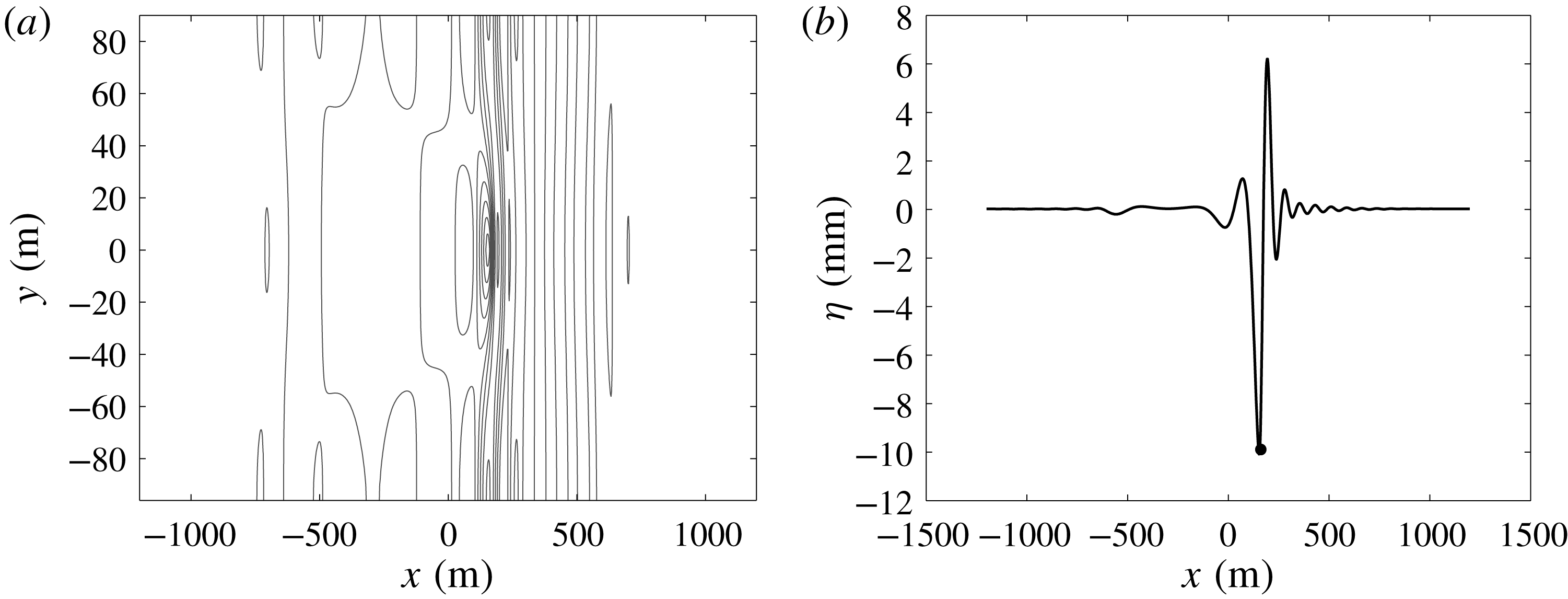
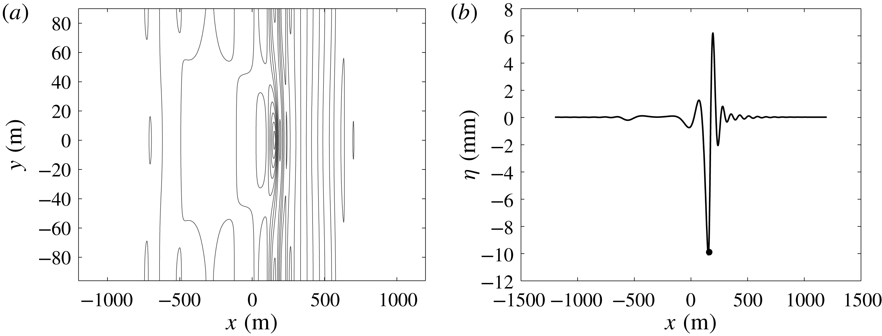
We also made some comparisons with the two-dimensional model (5.4), (5.5), which gave similar results. An example of a two-dimensional wave pattern is shown in figure 6 for the case when the load speed is $u=8.9~\text{m}~\text{s}^{-1}$ . In particular, it should be noted that the contours shown in the two-dimensional wave pattern in figure 6(a) are of very small amplitude. Examining the centre line of the wave deflection in (b), it becomes clear that the shadow zone discovered by Davys et al. (Reference Davys, Hosking and Sneyd1985) using the linear steady model is recovered in our nonlinear time-dependent model.

In the field campaign of Wilson (Reference Wilson1955), an ammunition truck was driven over the ice-covered Mille Lacs near Brainerd, Minnesota in the United States of America. The deflection of the ice cover was measured with a deflectometer, the depth at the measuring point was about $3.26~\text{m}$ , and the ice thickness was $0.61~\text{m}$ . The elastic modulus was estimated to be $9\times 10^{9}~\text{N}~\text{m}^{-2}$ (see table 1). The non-dimensional damping coefficient was taken to be $B=0.95$ . Figure 7 shows comparisons with these experimental data. The load speeds (from a to e) are $2.6~\text{m}~\text{s}^{-1}$ , $4.6~\text{m}~\text{s}^{-1}$ , $7.3~\text{m}~\text{s}^{-1}$ , $8.4~\text{m}~\text{s}^{-1}$ and $17.9~\text{m}~\text{s}^{-1}$ . The data are compared to numerical approximations of solutions to the two-dimensional model (5.4), (5.5). The match between experimental data and numerical approximation is superb for the two subcritical cases. For the third and fourth case, the match is not as good, but given a probably rather large uncertainty in the measurements, the comparison is overall fair.

Figure 8.

Comparison of numerical approximation of (5.4), (5.5) and experimental ice deflection records with two trucks driving at constant speed. The dashed black curves are the experimental data of Wilson (Reference Wilson1955), and the red dots indicate the $z$ -position of the two trucks used in these experiments at the time they pass the deflectometer. The blue curves represent the time series of the numerical approximation of (5.4), (5.5), taken at a measuring station corresponding to the position of the deflectometer in the field experiment. The blue dots represent the $z$ -position of the two loads as they pass the position where the time series is obtained.

Figure 8 shows comparisons with the experimental data of Wilson (Reference Wilson1955) pertaining to the two-truck experiments. In these runs, two trucks were driven over the ice at a fixed distance. The comparison with the numerical approximation of (5.4), (5.5) is quite good, and in particular better than the single-truck case.

Lastly, we consider the experimental work of Beltaos (Reference Beltaos1981) carried out on Cold Lake which is located on the Alberta–Saskatchewan provincial boundary in Canada. A truck was driven along a test track located about $800~\text{m}$ from shore. The water depth was approximately $4.3~\text{m}$ and the ice thickness was $0.59~\text{m}$ . The elastic modulus was estimated to be $4.9\times 10^{9}~\text{N}~\text{m}^{-2}$ (see table 1). Note that while the dispersion curve also has two critical values in this case, they are so close together that in practice there is only one critical load speed, which Beltaos determined experimentally to be approximately $V_{c}=7.3~\text{m}~\text{s}^{-1}$ .

Figure 9 shows comparisons of the numerical approximations of (5.4), (5.5) with the experimental data of Beltaos (Reference Beltaos1981). The load speeds (from a to c) are $4.4~\text{m}~\text{s}^{-1}$ , $8.0~\text{m}~\text{s}^{-1}$ and $13.9~\text{m}~\text{s}^{-1}$ . The first load speed is subcritical, while the second and third are supercritical. The comparison of the wave profile is qualitatively good, but the numerical simulation slightly underpredicts the maximum deflection of the ice sheet. Of course, as also pointed out by Beltaos (Reference Beltaos1981), there is considerable uncertainty in the measurements, and as in the cases above, the damping parameter has to be estimated based on the fit with the experiments. In this case, the non-dimensional damping coefficient was taken to be $B=1.05$ . For the near-critical case with load speed $V=1.1V_{c}=8.0~\text{m}~\text{s}^{-1}$ the two-dimensional wave crest pattern is shown in figure 10. Since the load speed is above the critical speed, one also expects a shadow zone in this case, and this can be seen in the wave crest pattern in figure 10(a), and in the centre line deflection in (b). The small trailing disturbances are transients which decay over time.

Figure 9.

Comparison of numerical approximation of (5.4), (5.5) and experimental ice deflection records. The dashed black curves are the experimental ice deflection records of Beltaos (Reference Beltaos1981), and the red dots indicate the $z$ -position of the truck as it passes the deflectometer. The blue curves represent time series of the numerical approximation of (5.4), (5.5), taken at a measuring point corresponding to the position of the deflectometer in the field experiments. The blue dots represent the $z$ -position of the numerically imposed load as it passes the measuring point.

Figure 10.

Numerical approximation of (5.4), (5.5) for constant load velocity $V=8.0~\text{m}~\text{s}^{-1}$ , such as in figure 9. (a) Shows the wave crest pattern, and (b) shows the deflection of the ice sheet along the centre line $y=0$ .

Beltaos (Reference Beltaos1981) also raised the interesting question of whether a changing load speed may have an impact on the response of the ice sheet. In particular, he noted that drivers have reported ice failures occurring in the case of sudden deceleration because of a perceived danger ahead. As will be shown presently, deceleration may indeed have an adverse effect on the stability of the ice sheet, as interference patterns may contribute to exceeding the critical strain beyond which failures are likely to occur.

Figure 11.

Comparison of numerical approximation of (4.8), (4.18) for constant load velocity $10~\text{m}~\text{s}^{-1}$ (a,c,e) and deceleration from $10~\text{m}~\text{s}^{-1}$ to $0~\text{m}~\text{s}^{-1}$ (b,d,f). (a,b) Show the evolution of the surface deflection at a measuring station at a fixed location. (c,d) Show the $z$ position of the load as a function of time. (e,f) Show the maximum relative strain as a function of time.

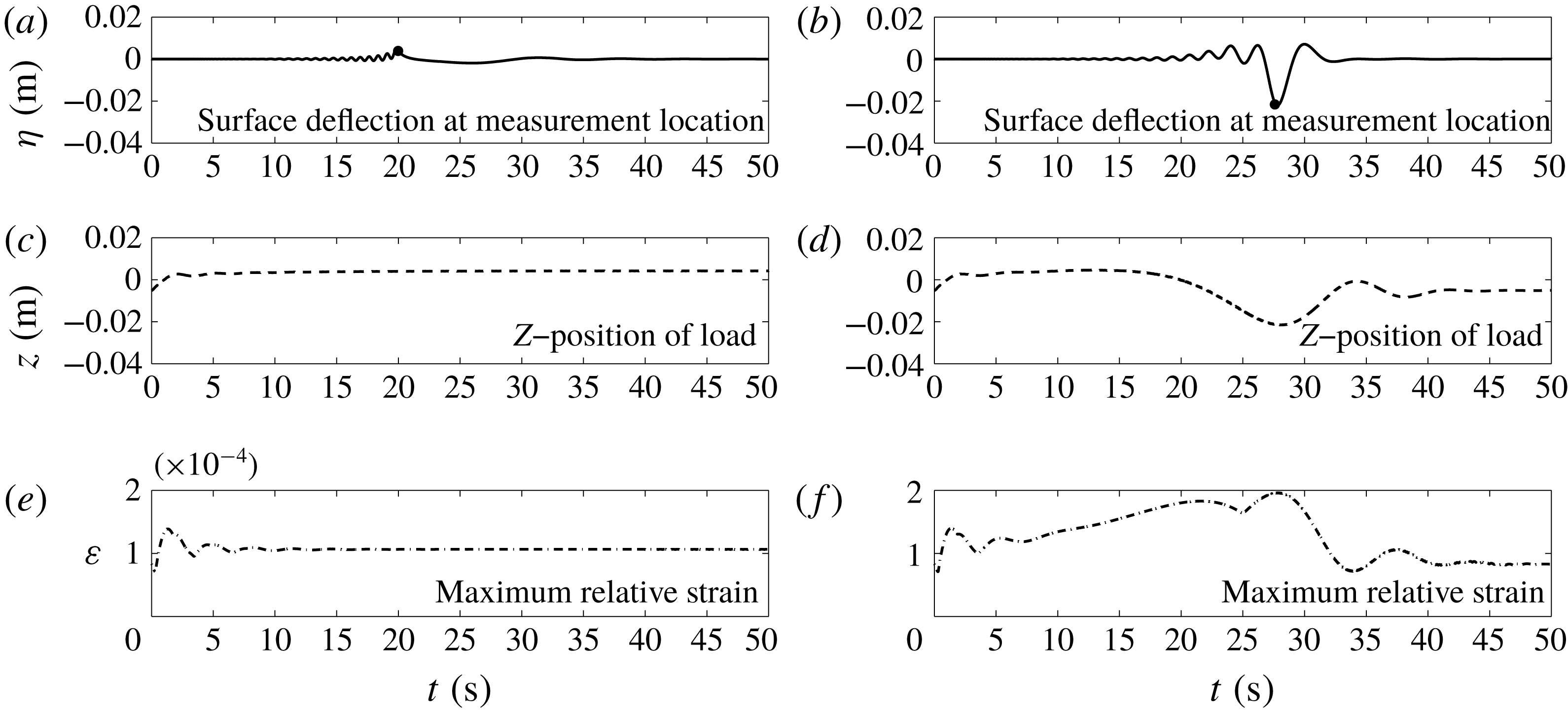
Figure 11 shows the development of the free surface for a load passing a measuring station. (a,c,e) show a load moving at constant speed. The curve in (a) depicts the deflection of the ice sheet at the measuring station, and the black dot indicates the time when the load passes the measuring station. Panel (c) shows the vertical position of the free surface at the point of the load, and (e) shows the maximum strain of the ice. The strain computed here is the linear or axial strain which is used in defining the bending moment of an elastic solid, and which can be measured experimentally using a strainmeter, such as explained in Davys et al. (Reference Davys, Hosking and Sneyd1985). According to Page & Părău (Reference Page and Părău2014) and references therein, the strain is approximated by the expression $\unicode[STIX]{x1D700}=(h/2)\unicode[STIX]{x1D702}_{xx}$ . The strain takes on large values at the beginning which is probably due to the impulsively started load (even though we made sure to use initial data corresponding to a static load so as to avoid a non-smooth start-up phase). Otherwise the maximum strain is of the order of $10^{-5}$ .

Figure 11(b,d,f) shows the case of a decelerating load. Panel (b) shows the development of the surface deflection at the measuring station, and the black dot indicates the time when the load passes the measuring station. We note that the surface deflection is larger by a factor of more than $10$ compared to the case of a load moving at constant speed. (d) Shows the corresponding vertical position of the load on the ice sheet, and the amplitude here is also larger by a factor of $10$ when compared to the case of constant propagation speed of the load. Finally, (f) shows the maximum strain in the ice sheet as a function of time. Here it must be noted that the maximum strain occurring at time $t=28$ is about $2\times 10^{-4}$ which is approaching the value $2.14\times 10^{-4}$ which was indicated in Goodman, Wadhams & Squire (Reference Goodman, Wadhams and Squire1980) as the critical strain where cracks may appear in the ice.

Maximum ice deflection and strain are summarized in table 2. Note that the values of maximum strain are slightly decreasing as the deceleration gets higher. From this trend, one may conclude that it is actually safer to brake swiftly rather than to brake slowly. The dependence of the maximum deflection and maximum strain on the load appears to be approximately linear.

The stark difference between the cases of constant load speed and decelerating load may be explained by constructive interference of waves of different phase speed created by the changing speed of the load. Indeed, as the load decelerates through the critical long-wave speed $\sqrt{gH}$ , it continuously excites gravity wave of smaller and smaller velocity. The analysis in Takizawa (Reference Takizawa1987) shows that gravity waves will generally trail the moving load. However, as the load velocity is getting smaller than the phase velocity of previously excited waves, the waves immediately catch up with the load, and through constructive interference an increasing bulge and trough traveling with the load are formed. Eventually, this process leads to the development of much larger surface deflections than could be expected with constant load speed. The time developments of the wave responses in the constant-speed case and in the decelerating are contrasted in figure 12.

Figure 12.

Comparison of numerical approximation of (4.8), (4.18) for constant load velocity $6.2~\text{m}~\text{s}^{-1}$ (a) and deceleration from $10~\text{m}~\text{s}^{-1}$ to $0~\text{m}~\text{s}^{-1}$ (b). The position of the load is indicated in magenta. Panel (a) shows gravity waves trailing the load, while (b) shows gravity waves continuously catching up with the load.

Table 2.

Maximum ice deflection and maximum strain rate during the deceleration of a light vehicle. The parameter values for this study have been taken from the experiments by Takizawa (Reference Takizawa1987), summarized in table 1.