




1 Introduction
High-power fiber lasers provide the beam quality and efficiency required for the most demanding tasks in manufacturing and defense[ Reference Nilsson and Payne 1 , Reference Jauregui, Limpert and Tünnermann 2 ]. However, with the rapid expansion of fiber laser applications, conventional single-wavelength systems increasingly encounter limitations in areas such as multi-material hybrid processing, coupled physical mechanisms and interference resilience under extreme conditions. Consequently, fiber laser technology is gradually evolving in the directions of high power, multi-wavelength and tunability[ Reference Fan, Liu, Wu, Wang, Yue, Wei and Liu 3 – Reference Liu, Zeng, Wang, Shi, Wu, Wang, Xi, Zhang, Ning and Xi 5 ]. Owing to their simple structure, compact size and wavelength scalability, dual-wavelength fiber lasers (DWFLs) have found widespread application in diverse fields such as industrial processing, spectrum measurement, optical communication, biomedicine and other areas[ Reference Jones and Watson 6 – Reference Liang, Xiao, Chen, Han, Lin, Huang and Huang 9 ]. In particular, for achieving high-power and stable dual-wavelength lasing output, ytterbium-doped fiber (YDF) is widely recognized as a highly desirable candidate gain medium, due to its wide gain bandwidth, compatibility with low-cost pump sources and relatively simple energy level structure[ Reference Hideur, Chartier, Özkul and Sanchez 10 – Reference Jawad, Salman, Anila, Benish and Karim 14 ].
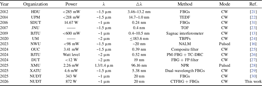
The realization of the aforementioned applications hinges on laser sources that provide stable and efficient dual-wavelength output. The wavelength extension can be achieved through nonlinear effects, and then independent dual-wavelength and even multi-wavelength output can be achieved by means of filtering[ Reference Nyushkov, Ivanenko, Vishnyakov, Kharauzov and Smirnov 15 – Reference Mirza, Ghafoor, Atieh, Kanwal and Qureshi 18 ]. Fiber Bragg gratings (FBGs) can also be utilized as filtering devices to achieve dual-wavelength or even multi-wavelength output[ Reference Kanwal, Atieh, Ghafoor, Sajid and Mirza 19 , Reference Mirza, Atieh, Kanwal, Ghafoor, Kausar, Imran, Almogren, Kanwal and Aziz 20 ]. Table 1 summarizes key research results for DWFLs across different wavelength bands. Prior research has leveraged diverse gain fibers and filtering techniques, resulting in limited low-power levels. In 2016, Liu et al. [ Reference Liu, Huang, Wei, Han, Huang and Liu 31 ] built a switchable single-wavelength/dual-wavelength polarization-maintaining YDF laser with FBGs, achieving a maximum output power of 14.67 W at 1118.912 and 1119.152 nm. Owing to superior power-handling capability, FBGs serve as a filter with significant potential for scaling the output power of fiber lasers. However, the output power achieved in this work remained low, and the wavelength spacing was narrow.
Literature review of DWFLs a .

Table 1 Long description
The table contains 14 rows, each representing a literature entry for DWFLs. Columns from left to right are: Year, Organization, Power, Lambda, Delta Lambda, Method, Mode, and Reference. Row 1: 2012, HYU, less than 285 mW, approximately 1.5 micrometers, 3.46 to 13.2 nanometers, F B G s, C W, reference 23. Row 2: 2014, U P M, less than 218 mW, approximately 1.5 micrometers, 14.7 to 1.0 nanometers, T E D F, C W, reference 24. Row 3: 2016, S D U T, 14.67 W, approximately 1 micrometer, 0.24 nanometers, F B G s, C W, reference 21. Row 4: 2017, J N U, not available, approximately 1.5 micrometers, 0.4 nanometers, T O F, C W, reference 25. Row 5: 2019, B J T U, less than 600 mW, approximately 1 micrometer, 0.4 to 10.5 nanometers, Sagnac interferometer, C W, reference 13. Row 6: 2020, U M, not available, approximately 2 micrometers, less than or equal to 183.6 nanometers, T B P F s, C W, reference 26. Row 7: 2023, N W U, less than 98 mW, approximately 1.5 micrometers, approximately 20 nanometers, N A L M, pulsed, reference 16. Row 8: 2024, O U C, 3.41 mW, approximately 1.5 micrometers, 56 nanometers, composite filter, C W, reference 27. Row 9: 2024, B J T U, watt level, approximately 2 micrometers, 0.52 nanometers, P M dash F B G plus T C dash D R C, C W, reference 28. Row 10: 2024, D U T, less than 12 W, approximately 2 micrometers, 19 nanometers, F B G plus F P filter, C W, reference 29. Row 11: 2025, X M U, 2.26 mW, 1.3 forward slash 1.4 micrometers, 96.16 nanometers, N P R, pulsed, reference 30. Row 12: 2025, X A T U, 4.6 mW, approximately 1.5 micrometers, 5.38 nanometers, dual-wavelength F B G s, C W, reference 31. Row 13: 2025, N U D T, 343 W, approximately 1 micrometer, 20 nanometers, F B G s, C W, reference 22. Row 14: 2026, N U D T, 872 W, approximately 1 micrometer, 20 nanometers, C T F B G plus F B G s, C W, this work. Table footnote defines abbreviations: T O F is time of flight, C W is continuous wave.
a HDU, Hangzhou Dianzi University; UPM, Universiti Putra Malaysia; SDUT, Shandong University of Technology; JNU, Jinan University; BJTU, Beijing Jiaotong University; UM, University of Malaya; NWU, Northwest University; OUC, Ocean University of China; DUT, Dalian University of Technology; XMU, Xiamen University; XATU, Xi'an Technological University; NUDT, National University of Defense Technology; TEDF, tapered erbium-doped fiber; TOF, tunable optical filter; TBPF, tunable bandpass filter; NALM, nonlinear amplifying loop mirror; PM-FBG, polarization-maintaining FBG; TC-DRC, three-coupler double-ring compound cavity; FP, Fabry-Perot; NPR, nonlinear polarization rotation.
To address the challenges posed by kilowatt-level high-power dual-wavelength or even multi-wavelength laser output, we have proposed and demonstrated a compact all-fiberized DWFL consisting of a cascade single-stage resonant cavity[ Reference Li, Ye, Li, Ding, Wu, Wang and Hua 30 ]. This architecture enables high-power single/dual-wavelength laser output at the 1 μm wavelength band, and provides a platform for systematically studying the nonlinear effects and their governing physical mechanism under high-power dual-wavelength lasing. In 2025, our research group reported a high-power resonant-cavity cascaded DWFL emitting at 1060 and 1080 nm, which achieved a maximum output power of 343 W[ Reference Li, Ye, Li, Ding, Wu, Wang and Hua 30 ]. The demonstration of stable hundred-watt-level operation marks significant progress, but the observation of nonlinear effects, differing from their single-wavelength counterparts, presents a notable challenge for further power scaling. In particular, a lack of systematic theoretical and experimental investigation exists into the nonlinear effects that arise specifically under high-power dual-wavelength operation.
In this work, a 1 μm band DWFL is constructed by cascading single-stage resonant cavities with FBGs. Simulations are conducted to study the effects of pump power distribution, the YDF length and the wavelength combination on the output performance, providing guidance for the structural parameter optimization. The output characteristics of the DWFL with different FBGs are experimentally compared and analyzed. The experimental results reveal that the stimulated Raman scattering (SRS) can be suppressed by the FBGs with wider bandwidth, while the incorporation of a chirped and tilted fiber Bragg grating (CTFBG) suppresses noise in other wavelength bands. When the CTFBG is positioned at the output, the signal-to-noise ratio (SNR) reaches its maximum. Based on FBGs with wider bandwidth, the dual-wavelength laser output with a power of 30.76 W at 1060 nm and 839.81 W at 1080 nm has been achieved.
2 Theoretical analysis and numerical simulations
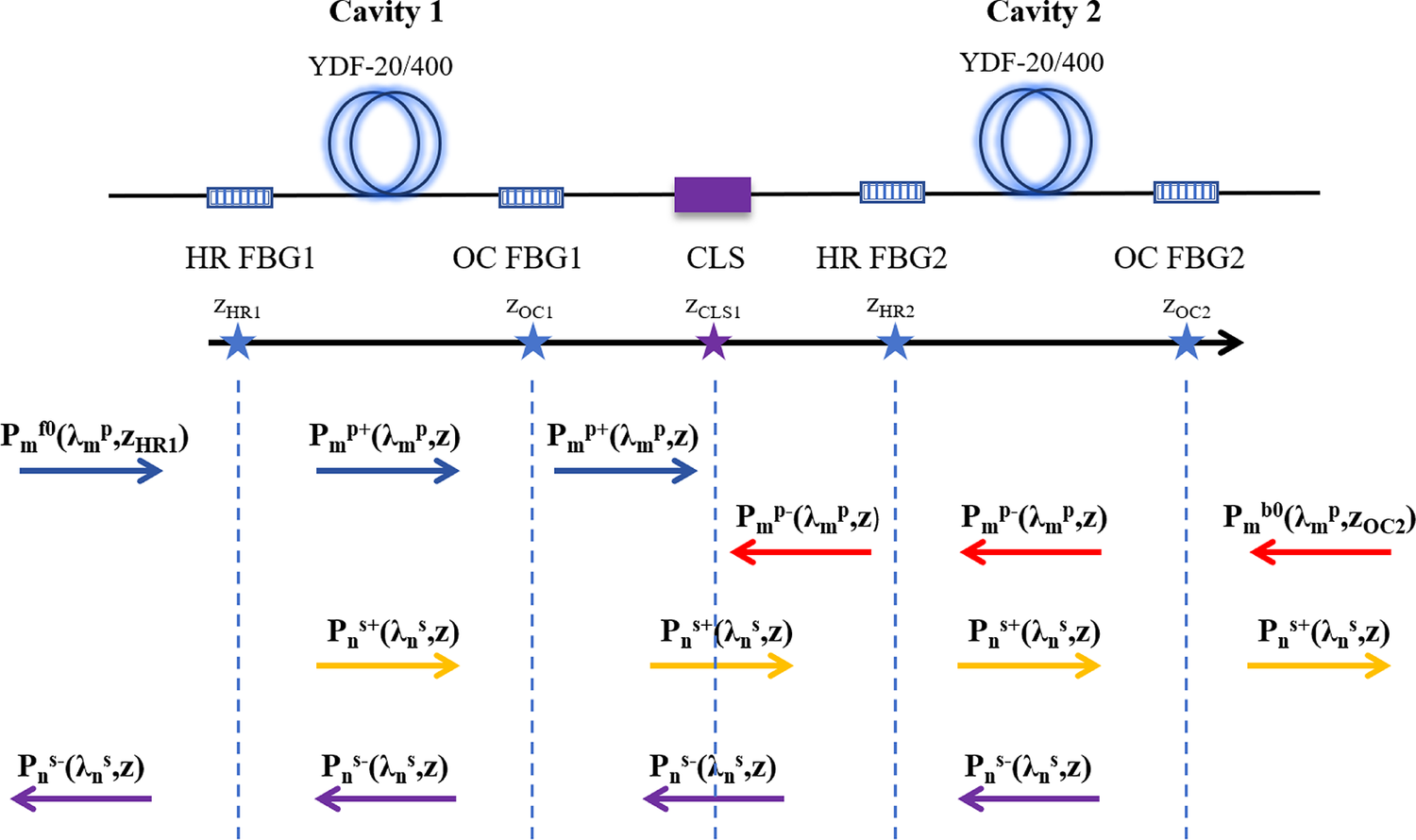
A theoretical model was established using steady-state rate equations, which include SRS and amplified spontaneous emission (ASE) effects, as well as the boundary conditions specific to the cascaded cavity configuration[ Reference Wu, Yan, Li, Li, Chen, Gong and Xiao 32 – Reference Várallyay and Jasapara 34 ]. The power throughout the DWFL structure can be simulated by solving its rate equations. The upper lasing level population, signal power and pump power can be computed based on Equations (1)–(3). The boundary conditions are shown in the Figure 1 and Equations (4) and (5), which primarily address the influence of two pairs of FBGs while implementing simplified pump filtering:


Schematic diagram of boundary conditions for the DWFL.

Figure 1 Long description
From left to right, the diagram displays two fiber cavities labeled Cavity 1 and Cavity 2, each containing a Y D F dash 20 forward slash 400 coil. Between and within the cavities are labeled sections: H R F B G 1, O C F B G 1, C L S, H R F B G 2, and O C F B G 2. Blue stars mark boundary points z H R 1, z O C 1, z C L S 1, z H R 2, and z O C 2 along a horizontal axis. At each boundary, arrows indicate the direction of power terms: P sub m super f 0 open parenthesis lambda sub m super p comma z sub H R 1 close parenthesis points right at z H R 1; P sub m super p plus open parenthesis lambda sub m super p z close parenthesis points right at z O C 1 and z C L S 1; P sub m super p minus open parenthesis lambda sub m super p z close parenthesis points left at z H R 2 and z O C 2; P sub m super b 0 open parenthesis lambda sub m super p z sub O C 2 close parenthesis points right at z O C 2. For signal terms, P sub n super s plus open parenthesis lambda sub n super s z close parenthesis points right at z O C 1, z C L S 1, z H R 2, and z O C 2; P sub n super s minus open parenthesis lambda sub n super s z close parenthesis points left at z H R 1, z O C 1, z C L S 1, and z H R 2. Arrow colors distinguish power types: blue for pump forward, red for pump backward, yellow for signal forward, and purple for signal backward. The central section is labeled C L S and separates the two cavities.
where the plus and minus superscripts represent propagation along the positive or the negative direction, the p and s subscripts represent the pump and signal light, respectively, N 0 is the total population, N 2 is the upper lasing level population, with spontaneous lifetime of τ, σa and σe are the absorption and emission cross-sections, respectively, Γp and Γs are the overlap factor of the pump and signal, respectively, A eff is effective mode area of the fiber and g R is the Raman gain coefficient.


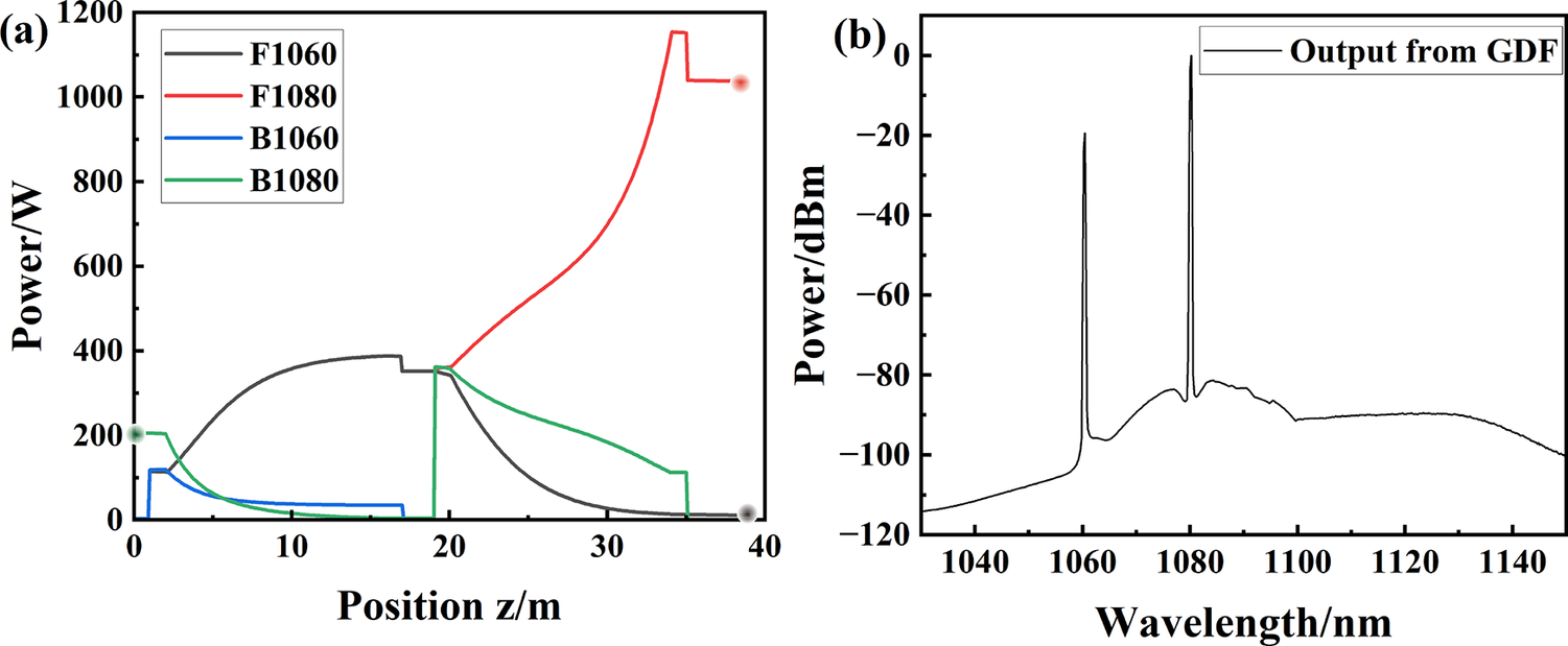
Based on the aforementioned model establishment for simulation, the parameters were configured as shown in Table 2. The power distribution of the signal laser of 1060 and 1080 nm and the output spectrum obtained through simulation are as shown in Figure 2. At the output port, the output power of the 1060 nm component exhibits a relatively low level, whereas the backward-propagating power is dominated by the 1080 nm component. No 1100 nm light is observed in the spectrum. Under forward and backward pump powers of 573 and 819 W, respectively, the simulation predicts a total output power of 1017.36 W, comprising 10.41 W at 1060 nm and 1006.95 W at 1080 nm. The backward-propagating power is 196.66 W, mainly consisting of 1080 nm power.
Basic parameters and values in the simulation a .

Table 2 Long description
Starting from the top row, the left column lists ‘Signal wavelength of cavity 1/2’ with values ‘1060/1080 nanometers’, and the right column lists ‘Total pump power’ as ‘Variable’. The next row presents ‘Pump wavelength’ as ‘976 nanometers’ on the left and ‘Pump absorption coefficient’ as ‘0.44 decibel per meter at 915 nanometers’ on the right. The third row shows ‘Reflectivity/3 decibel bandwidth of H R dash F B G 1/2’ with values ‘99 percent/4 nanometers’ on the left, and ‘Core/cladding diameter of Y D F’ as ‘20/400 micrometers’ on the right. The fourth row lists ‘Reflectivity/3 decibel bandwidth of O C dash F B G 1/2’ with values ‘10 percent/2 nanometers’ on the left, and ‘Active fiber length of cavity 1/2’ as ‘Variable’ on the right. The fifth row presents ‘N A’ as ‘0.061’ on the left and ‘Spontaneous lifetime’ as ‘840 microseconds’ on the right. The final row lists ‘Pump configuration’ as ‘Bidirectional pump’ on the left, with the right columns showing dashes, indicating no parameter or value.
a HR-FBG, high-reflection FBG; OC-FBG, output-coupler FBG.
Simulation results of the theoretical model of the DWFL (forward pump: 573 W; backward pump: 819 W). (a) Power distribution. (b) Output spectrum.

Figure 2 Long description
The left panel shows a line graph with x-axis labeled Position z slash m from 0 to 40 and y-axis labeled Power slash W from 0 to 1200. Four curves are plotted: F 1060 in black, F 1080 in red, B 1060 in blue, and B 1080 in green. F 1060 starts near 200 W, rises to a peak near 400 W at z equals 20, then drops to zero by z equals 40. F 1080 starts at zero, rises steeply after z equals 20, and peaks above 1000 W at z equals 40. B 1060 and B 1080 both start near 200 W, decrease rapidly, and approach zero by z equals 20. The right panel shows a line graph with x-axis labeled Wavelength slash n m from 1040 to 1140 and y-axis labeled Power slash d B m from negative 120 to 0. The curve labeled Output from G D F displays two sharp peaks at approximately 1060 n m and 1080 n m, with a broad lower background between 1040 and 1140 n m.
2.1 Influence of pump power on output characteristics
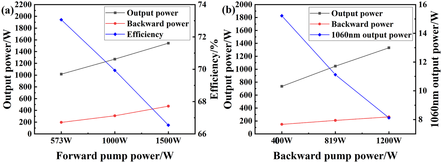
In previous experiments under bidirectional pumping conditions, both the sequence and relative proportion of forward and backward pump power were found to influence the output characteristics. The influence of the pump power variation on the output power was numerically investigated, and the results are shown in Figure 3. Maintaining the backward pump power at 819 W and increasing the forward pump power leads to a rapid increase in the backward-propagating power, accompanied by a reduction in conversion efficiency. Conversely, when the forward pump power was fixed at 623 W, increasing the backward pump power produced only a modest increase in backward-propagating power. In this case, the overall conversion efficiency improved with higher pump power, but the output at 1060 nm decreased. These results indicate that the pump power ratio can be systematically optimized based on simulation predictions.
Output power variation with the pump power. (a) Output power, backward power and efficiency variation with forward pump power. (b) Output power, backward power and 1060 nm output power variation with the backward pump power.

Figure 3 Long description
The left panel shows output power in watts and efficiency in percent versus forward pump power in watts. The x-axis ranges from 573 to 1500 watts. Output power (black squares) increases from about 1100 to 1800 watts. Backward power (red circles) rises from about 150 to 400 watts. Efficiency (blue diamonds) decreases from about 73 percent to 67 percent. The right panel plots output power and 1060 nanometer output power in watts versus backward pump power in watts, with the x-axis from 400 to 1200 watts. Output power (black squares) increases from about 900 to 1500 watts. Backward power (red circles) rises from about 100 to 300 watts. 1060 nanometer output power (blue diamonds) decreases from about 15 to 2 watts.
2.2 Influence of YDF length on output characteristics
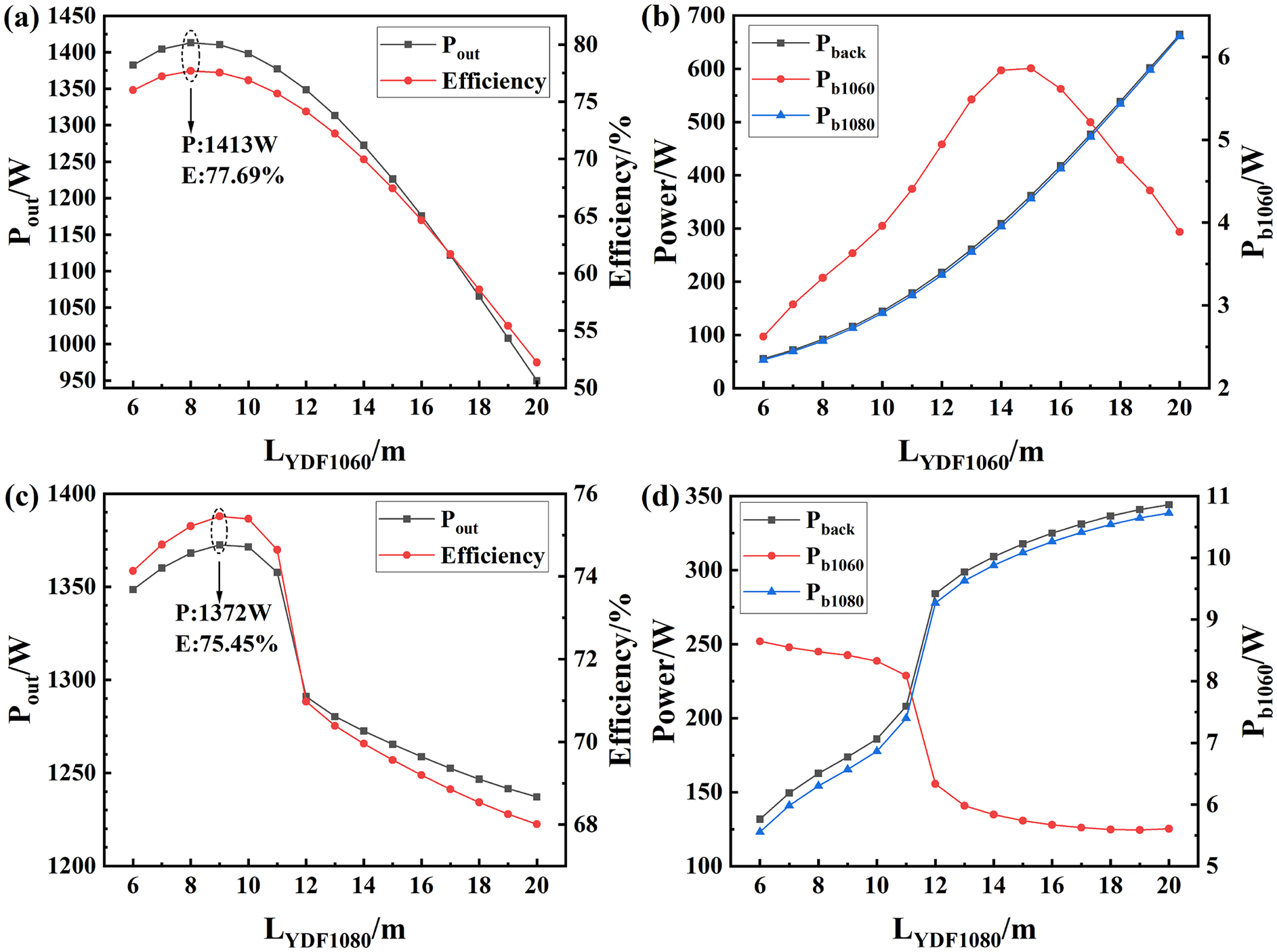
Previously, the length of the YDF was calculated based on the absorption coefficient of the pump light by the YDF. However, there are two sections of YDFs in this structure, and the lengths of the YDFs have a significant impact on the backward-propagating power. By varying the YDF length, the maximum value of the output power can be observed, which enables the identification of the optimal fiber length[ Reference Mirza, Atieh, Kanwal and Ghafoor 35 ]. Figure 4 presents the impact of varying the lengths of each YDF section on output power, efficiency and backward-propagating power. Increasing the length of each YDF section, the output power and conversion efficiency rise to a peak before declining. Compared with the fiber laser with a section of YDF as the gain medium, this configuration is more sensitive to the length variations of the two sections of fibers. This is caused by the opposite transmission of the signal light generated by the two cavities. The 1060 nm light is absorbed when passing through the 1080 nm cavity. The 1080 nm light passes through the 1080 nm high-reflection FBG (HR-FBG), then propagates in the reverse direction and is amplified by the 1060 nm cavity. It is output in the form of backward-propagating light, thereby affecting the output power. It is noteworthy that increasing the length of the 1080 nm resonator YDF from 11 to 12 m results in a sharp drop in output power, a phenomenon that warrants further investigation. The length of the 1060 nm resonator YDF has a more pronounced impact on the output power. When the forward pump power is 1000 W, the backward pump power is 819 W. The length of the YDF in the 1080 nm resonator is 14 m, while the length of the YDF in the 1060 nm resonator is reduced from 16 to 8 m. The simulation results show a 237 W output power increase with 13.05% efficiency enhancement. Based on the simulation results of the YDF length and the calculation results of the absorption coefficient for the pump light, we select the appropriate length of the YDF.
Output power variation with the YDF length (forward pump: 1000 W; backward pump: 819 W). (a) Output power and efficiency variation with the 1060 nm resonator YDF. (b) Backward power variation with the 1060 nm resonator YDF. (c) Output power and efficiency variation with the 1080 nm resonator YDF. (d) Backward power variation with the 1080 nm resonator YDF.

Figure 4 Long description
Panel a, top-left, plots L sub Y D F 1060 in meters on the x-axis, P sub out in watts on the left y-axis, and Efficiency in percent on the right y-axis. Two lines are shown: black squares for P sub out and red circles for Efficiency. Both peak near L sub Y D F 1060 equals 9 meters, with P sub out at 1413 watts and Efficiency at 77.69 percent, then decrease as length increases. Panel b, top-right, plots L sub Y D F 1060 in meters on the x-axis, Power in watts on the left y-axis, and P sub b 1060 in watts on the right y-axis. Three lines are shown: black squares for P sub back, red circles for P sub b 1060, and blue triangles for P sub b 1080. All increase with length, but P sub b 1060 peaks near 15 meters then declines, while P sub back and P sub b 1080 rise steadily. Panel c, bottom-left, plots L sub Y D F 1080 in meters on the x-axis, P sub out in watts on the left y-axis, and Efficiency in percent on the right y-axis. Black squares for P sub out and red circles for Efficiency both peak near 9 meters, with P sub out at 1372 watts and Efficiency at 75.45 percent, then decrease. Panel d, bottom-right, plots L sub Y D F 1080 in meters on the x-axis, Power in watts on the left y-axis, and P sub b 1060 in watts on the right y-axis. Black squares for P sub back and blue triangles for P sub b 1080 increase with length, while red circles for P sub b 1060 decrease after 10 meters. Legends and axis labels are present in each panel.
2.3 Influence of dual-wavelength combination on output characteristics
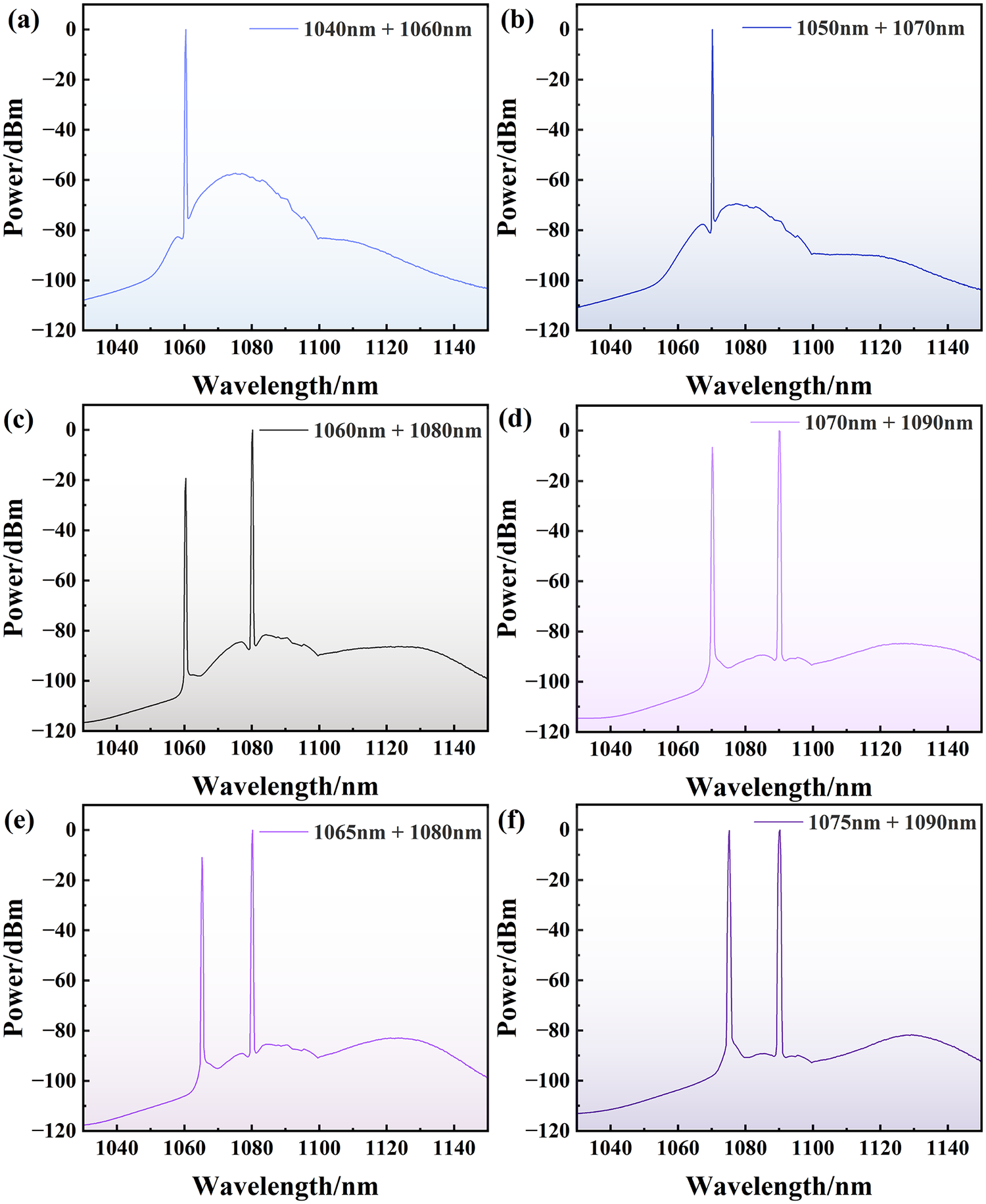
Motivated by the relatively low output power at 1060 nm in the current simulation, different wavelength combinations were explored, and the dependence of the output characteristics on these combinations was subsequently evaluated. The corresponding spectra are shown in Figure 5. Firstly, the wavelength combination is shifted towards the shorter wavelength. For the combinations (1040 nm + 1060 nm) and (1050 nm + 1070 nm), only the long wavelength laser can be observed in the spectra, which is not conducive to the simultaneous output of dual-wavelength lasers. Comparatively, the spectra of the (1060 nm + 1080 nm) and (1070 nm + 1090 nm) combinations show the simultaneous output of dual-wavelength lasers. Notably, the intensity of the short wavelength laser has increased relatively in the spectrum of the (1070 nm + 1090 nm) combination. The wavelength spacing was subsequently adjusted. When the wavelength spacing was increased, only a long wavelength laser can be observed in the spectra. Then, the wavelength spacing was reduced. For the (1065 nm + 1080 nm) and (1075 nm + 1090 nm) combinations, it could be observed that the intensity of the short wavelength laser in the output spectra further increased, which is beneficial for enhancing the output power of the short wavelength. When using the (1075 nm + 1090 nm) combination, with a forward pump power of 1000 W and a backward pump power of 819 W, the output power reaches 1531 W. Compared with the (1060 nm + 1080 nm) combination, it increases by 259 W, and the backward-propagating power decreases to 24 W. The power of 1075 nm light is 643 W, and the power of 1090 nm light is 888 W. The results show that the short wavelength power has significantly increased.
Comparative spectra under different wavelength combinations (forward pump: 1000 W; backward pump: 819 W). (a) 1040 and 1060 nm. (b) 1050 and 1070 nm. (c) 1060 and 1080 nm. (d) 1070 and 1090 nm. (e) 1065 and 1080 nm. (f) 1075 and 1090 nm.

Figure 5 Long description
Panel a, top left, plots power in d B m versus wavelength from 1040 to 1140 nanometers for 1040 plus 1060 nanometers, showing a sharp peak near 1060 nanometers and broad background. Panel b, top center, for 1050 plus 1070 nanometers, shows a similar sharp peak near 1070 nanometers. Panel c, top right, for 1060 plus 1080 nanometers, displays two distinct sharp peaks at 1060 and 1080 nanometers. Panel d, bottom left, for 1070 plus 1090 nanometers, also shows two sharp peaks at 1070 and 1090 nanometers. Panel e, bottom center, for 1065 plus 1080 nanometers, shows peaks at 1065 and 1080 nanometers. Panel f, bottom right, for 1075 plus 1090 nanometers, shows peaks at 1075 and 1090 nanometers. All panels have the same axes: x axis labeled Wavelength in nanometers, y axis labeled Power in d B m, ranging from minus 120 to 0 d B m. The spectral background and peak intensities vary between panels, illustrating how different wavelength combinations affect the output spectra.
Guided by the above simulation results of the pump power distribution, YDF length and wavelength combination, the (1075 nm + 1090 nm) combination was selected, and the YDF lengths were set to 12 and 14 m, respectively. When the forward pump power was 2000 W and the backward pump power was 3000 W, the output power obtained through simulation reached 4158 W. This comprises 322 W at 1075 nm while maintaining backward-propagating power at 104 W, demonstrating significant potential for power scaling in this configuration. However, the 1090 nm quantum defect is larger, resulting in a significant increase in heat load. In addition, the gain curve of the YDF reaches its peak around 1080 nm, while the gain coefficient at 1090 nm is relatively low. Therefore, the (1060 nm + 1080 nm) combination was maintained for the subsequent experiments.
3 Experimental implementation
3.1 Experimental setup
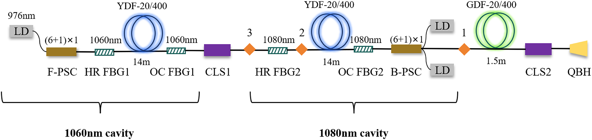
Figure 6 shows the configuration of the DWFL. For comparison with previous experimental results, the DWFL is constructed by cascading two resonant cavities with central wavelengths of 1060 m and 1080 nm. To suppress the SRS phenomenon observed in previous experiments[ Reference Li, Ye, Li, Ding, Wu, Wang and Hua 30 ], FBGs with a wider 3 dB bandwidth were utilized. The current and previous experimental setups are designated as narrow bandwidth grating configuration and broad-bandwidth grating configuration, respectively.
Schematic diagram of the DWFL with 1060–1080 nm resonator cascade configuration.

Figure 6 Long description
Starting at the far left, a 976 nanometer LD connects to a F-P S C, followed by H R F B G 1 and O C F B G 1, all labeled 1060 nanometer. This section includes a Y D F dash 20 slash 400 fiber coil, 14 meters long, and is marked as the 1060 nanometer cavity. The path continues through C L S 1, then H R F B G 2, and a second 14 meter Y D F dash 20 slash 400 coil, now labeled 1080 nanometer, forming the 1080 nanometer cavity. O C F B G 2 follows, then a B-P S C, with additional L D pump sources indicated by (6 plus 1) times 1. The path enters a G D F dash 20 slash 400 coil, 1.5 meters, then C L S 2, and ends at Q B H. All major components are labeled, with arrows indicating the direction of optical flow from left to right.
The 1060 nm cavity involves a pair of FBGs, including an output-coupler FBG (OC-FBG#1) and HR-FBG (HR-FBG#1). The central wavelength of HR-FBG#1 is 1060.05 nm, the reflectivity is 99.75% and the 3 dB bandwidth is about 4.01 nm. The central wavelength of OC-FBG#1 is 1060.02 nm, the reflectivity is 9.64% and the 3 dB bandwidth is about 2.04 nm. The 1080 nm cavity involves a pair of FBGs (OC-FBG#2 and HR-FBG#2) with the central wavelengths of 1080.66 and 1080.53 nm, respectively. The reflectivity of HR-FBG#2 is 99.91% with a 3 dB bandwidth of 3.84 nm. The reflectivity of OC-FBG#2 is 9.97% with a 3 dB bandwidth of 1.97 nm. A set of 976 nm laser diode (LD) modules with the maximum rated power of 780 W is coupled into the 1060 nm cavity through a (6 + 1) × 1 forward pump and signal combiner (F-PSC). In addition, two sets of 976 nm LD modules with the maximum rated power of 780 and 650 W are coupled into the 1080 nm cavity through a (6 + 1) × 1 backward pump and signal combiner (B-PSC). The gain fibers in both cavities are 20/400 μm YDFs with the length of 14 m, the cladding absorption coefficient is 0.44 dB/m at 915 nm and the numerical aperture (NA) values of the core and clad are respectively up to 0.061 and 0.46.
To suppress parasitic 1100 nm emission observed in previous experiments, a CTFBG was sequentially inserted at positions labeled 1–3, as shown in Figure 6. The central wavelength of the CTFBG is 1102.0 nm, the wavelength coverage is more than 15 nm and the suppression ratio is around 18 dB. For the suppression of backward-propagating power of the 1060 nm resonator side, HR-FBG#3 is added at the position labeled 3, with the central wavelength of 1080.04 nm, reflectivity of 99.55% and 3 dB bandwidth of 4.04 nm. After the B-PSC, the signal light passes cladding light stripper #2 (CLS#2) and is output from a quartz block holder (QBH). Two CLSs (CLS#1 and CLS#2) in the configuration are utilized to dump the cladding light in the delivery fiber.
In the experiment, the output power, spectra and time-domain changes of power are measured by a power meter, an optical spectrum analyzer and a photodetector, respectively.
3.2 Laser performance of the broad bandwidth configuration
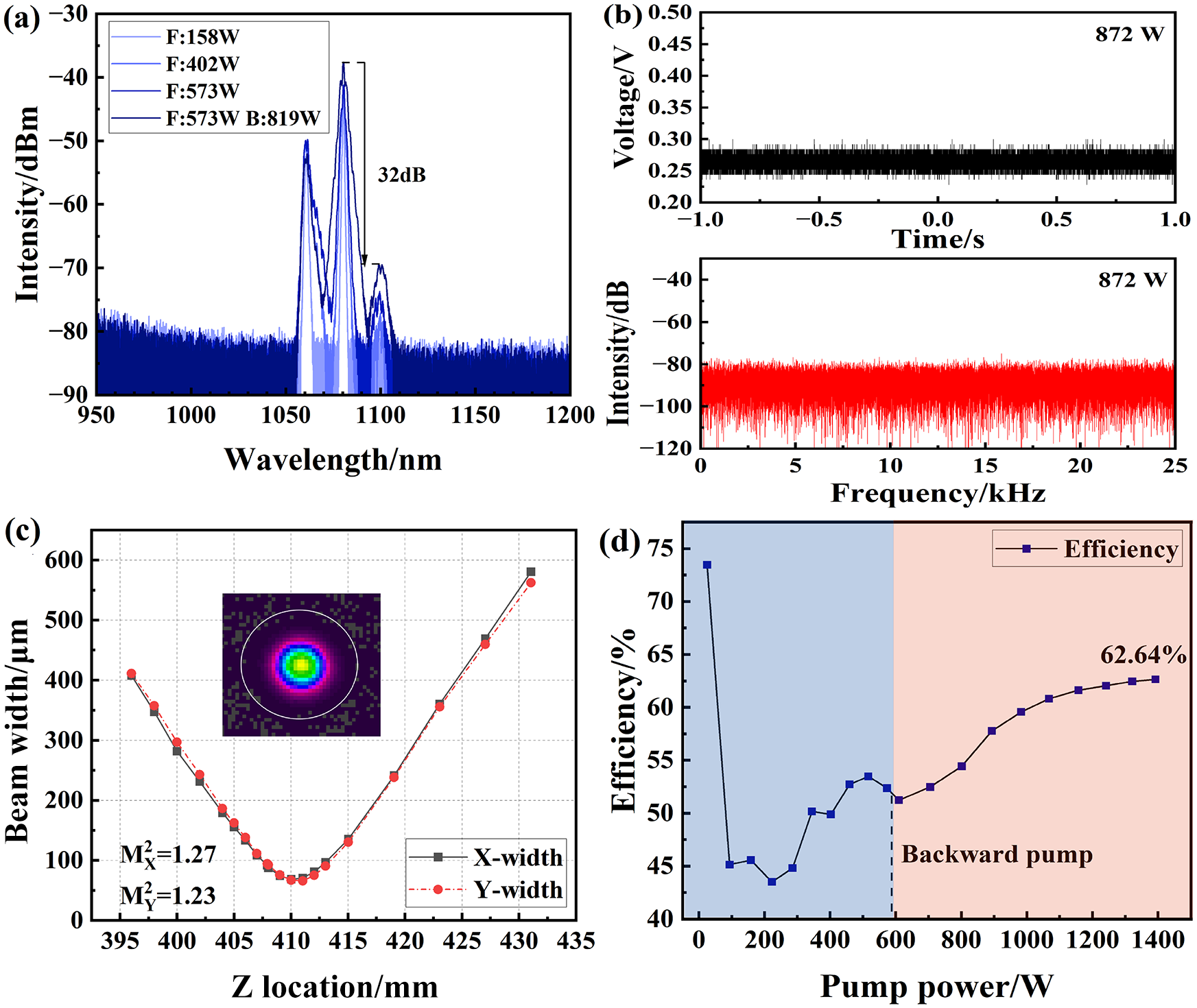
In the DWFL with 1060–1080 nm cascaded resonator configuration, for clarity, the co-pumping of the 1060 nm resonator side is termed forward pumping, while the counter-pumping of the 1080 nm resonator side is termed backward pumping. Figure 7 shows the output characteristic corresponding to the configuration with broad-bandwidth gratings. As shown, when the forward pump power is 158 W, 1060 and 1080 nm light can be observed in the spectrum. When the forward pump power is increased to 402 W, 1100 nm wavelength light is observed in the spectra. The underlying mechanism of this emission is likely associated with the four-wave mixing effect[ Reference Agrawal 36 ]. With the increasing of pump power, the bandwidth of different wavelengths increases, and their wavelength range overlaps. Compared with the simulation results, 1100 nm light can be observed, and the spectral broadening phenomenon is more pronounced. This might be caused by the fact that the rate equation neglects the four-wave mixing effect. The SNR of 1080 and 1100 nm is 32 dB. From the output power distribution, the 1080 nm component dominates, reflecting the stronger optical gain associated with the absorption and emission cross-sections of ytterbium ions.
Output characteristic of the DWFL with a broad-bandwidth grating (forward pump: 573 W; backward pump: 819 W). (a) Output spectra. (b) Temporal signal and Fourier spectrum. (c) Beam quality. (d) Conversion efficiency.

Figure 7 Long description
Panel a at top left is a line graph with x axis labeled Wavelength in nanometers from 950 to 1200 and y axis labeled Intensity in d B m from minus 90 to minus 30. Four traces are shown for F 158 W, F 402 W, F 573 W, and F 573 W B 819 W. The main peaks are near 1070 to 1100 nanometers, with a 32 d B difference marked between peak and baseline. Panel b at top right contains two plots. The upper plot shows Voltage in V versus Time in seconds from minus 1 to 1, with a flat trace at 872 W. The lower plot shows Intensity in d B versus Frequency in k H z from 0 to 25, also at 872 W, with a flat noise-like trace. Panel c at bottom left is a line graph with x axis Z Location in millimeters from 395 to 435 and y axis Beam Widths D 4 sigma in micrometers from 0 to 600. Two traces, X width and Y width, show a minimum near 410 millimeters. Inset is a color beam profile with a central bright spot. M x squared equals 1.27, M y squared equals 1.23. Panel d at bottom right is a line graph with x axis Pump power in W from 0 to 1400 and y axis Efficiency percent from 40 to 75. The curve shows efficiency dropping then rising, reaching 62.64 percent at highest power. The region above 700 W is shaded and labeled Backward pump.
At forward and backward pump powers of 573 and 819 W, respectively, the total output power reaches 872 W, comprising 31 W at 1060 nm and 840 W at 1080 nm. During the experiment, there are no signs of transverse mode instability (TMI) phenomena observed. The M 2 value is 1.25, achieving near-single-mode output. From Figure 7(d), the efficiency increases progressively with pump power, which can be attributed to the wavelength shift of the LD emission as the drive current rises. This spectral shift enhances the overlap with the absorption band of the gain medium, thereby improving pump absorption. As a result, the conversion efficiency continues to increase until reaching a steady-state value.
A comparison with the simulation output power is shown in Table 3. The experimental results closely validate the predictive accuracy of the simulation model. The marginally lower measured output power can be primarily attributed to unaccounted losses in the simulation model.
Comparison of output power between the simulation and experiment.

Table 3 Long description
From left to right, the columns are labeled P/W, P sub 1060 all over W, P sub 1080 all over W, P sub r all over W, P sub b all over W, P sub b1060 all over W, and P sub b1080 all over W. The first row presents simulation values: 1017.36 for P/W, 10.41 for P sub 1060 all over W, 1006.95 for P sub 1080 all over W, 7.83 times 10 to the minus 5 for P sub r all over W, 196.66 for P sub b all over W, 3.10 for P sub b1060 all over W, and 193.56 for P sub b1080 all over W. The second row presents experiment values: 872 for P/W, 30.76 for P sub 1060 all over W, 839.81 for P sub 1080 all over W, 1.40 for P sub r all over W, 182 for P sub b all over W, and dashes for P sub b1060 all over W and P sub b1080 all over W, indicating missing data.
Collectively, the output power of the DWFL is further improved by replacing the FBGs with wider 3 dB bandwidth. However, the light intensity of 1100 nm in the spectra is stronger. In the subsequent experiments, a CTFBG was added to the broad-bandwidth grating configuration for the suppression of 1100 nm light.
3.3 Laser performance of the broad bandwidth configuration with the CTFBG
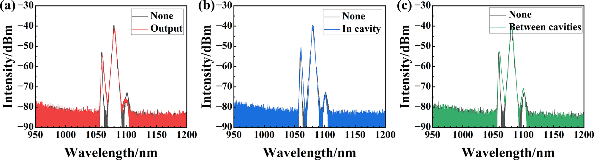
Figure 8 compares the output spectra obtained before and after the introduction of the CTFBG within the broadband grating configuration. As shown in Figure 8(a), placing the CTFBG at the output end effectively suppresses the 1100 nm component, with the SNR of 1080 and 1100 nm increasing from 32 to 35 dB. This clearly demonstrates the suppression capability of the CTFBG for parasitic 1100 nm light.
Output spectra of the DWFL with the CTFBG (forward pump: 573 W; backward pump: 819 W). (a) CTFBG at output. (b) CTFBG in the cavity. (c) CTFBG between cavities.

Figure 8 Long description
From left to right, panel a shows two overlaid spectra labeled None in black and Output in red, with Output displaying higher intensity peaks near 1060 nanometers and 1100 nanometers. Panel b overlays None in black and In cavity in blue, with In cavity showing similar peak positions but slightly lower intensities. Panel c overlays None in black and Between cavities in green, with Between cavities showing peaks at the same wavelengths but with reduced intensity compared to Output. All panels have x axes labeled Wavelength slash n m from 950 to 1200 and y axes labeled Intensity slash d B m from negative 90 to negative 30. Legends are in the upper right of each panel.
To further examine the influence of the CTFBG placement on DWFL output characteristics, the grating was alternatively positioned within the 1080 nm cavity and in the inter-cavity region. Figures 8(b) and 8(c) respectively display the spectral profiles before and after inserting the CTFBG into the 1080 nm cavity and the inter-cavity region. As shown in the figure, the light intensity of 1100 nm light and the SNR of 1080 nm light and 1100 nm light do not change significantly. The suppression effect of the CTFBG on 1100 nm light is not obvious. A plausible explanation is that the CTFBG also imposes attenuation on the 1080 nm signal, and this effect is strongly dependent on its position within the cavity structure, thereby leading to the observed differences in SNR between the 1080 and 1100 nm components.
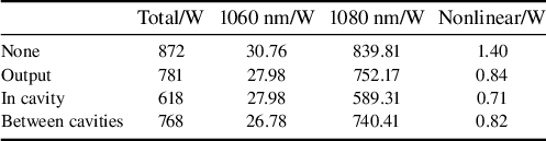
Integrating the spectra in different wavelength ranges, the output power in different wavelength ranges can be obtained. The optical power distribution of different configurations is shown in Table 4. It can be seen that the output power of different configurations degrades variably under the same pump power. When the CTFBG is set in the 1080 nm cavity, it drops to the lowest value of 618 W. For different configurations, the power of the nonlinear wavelength range is reduced by nearly half but no more than 1 W after adding the CTFBG. The power reduction of 1060 nm is not obvious, and the total power reduction mainly originates from the reduction of 1080 nm power. These results indicate that while the CTFBG effectively suppresses parasitic emission around 1100 nm, it also introduces a noticeable impact on the 1080 nm light. In future work, the wavelength coverage of the CTFBG can be controlled to be less than 10 nm by appropriately reducing the tilted angle, chirp rate and grating length[ Reference Wang, Li, Liu, Wang, Gu and Xu 37 ]. Based on recent reports on the application of CTFBGs in high-power fiber lasers, an insertion loss of less than or equal to 0.15 dB and a suppression ratio of more than or equal to 20 dB for the unwanted wavelength (~1100 nm) could be demonstrated[ Reference Li, Ye, Wang, Wu, Gao, Rao, Tian, Xi, Chen, Wang and Chen 38 , Reference Jiao, Shu, Shen, Guan, Yang and Zhu 39 ].
Output power distribution of different configurations.

Table 4 Long description
The table has five columns: configuration, total power in watts, 1060 nanometer power in watts, 1080 nanometer power in watts, and nonlinear power in watts. The four configurations listed from top to bottom are None, Output, In cavity, and Between cavities. For None: total power is 872, 1060 nanometer is 30.76, 1080 nanometer is 839.81, nonlinear is 1.40. For Output: total power is 781, 1060 nanometer is 27.98, 1080 nanometer is 752.17, nonlinear is 0.84. For In cavity: total power is 618, 1060 nanometer is 27.98, 1080 nanometer is 589.31, nonlinear is 0.71. For Between cavities: total power is 768, 1060 nanometer is 26.78, 1080 nanometer is 740.41, nonlinear is 0.82. The highest total and 1080 nanometer power values are in the None configuration, while the lowest values are in the In cavity configuration. Nonlinear power is lowest in the In cavity configuration and highest in the None configuration.
From the spectra and power results, the SNR of 1080 nm light and 1100 nm light can be improved due to the suppression effect of the CTFBG on the 1100 nm light. However, the CTFBG also has an inhibitory effect on 1080 nm light, which significantly reduces the output power. The results indicate potential for further optimization by adjusting the parameters of the CTFBG.
3.4 Laser performance of the broad bandwidth configuration with HR-FBG#3
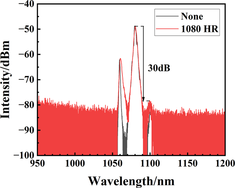
After replacing the FBGs with a wider 3 dB bandwidth, the backward-propagating power of the 1060 nm resonant cavity decreases under the same pump power. Therefore, it is considered to add a 1080 nm FBG to the broad-bandwidth grating configuration. The spectra of the broad-bandwidth grating configuration and the configuration with the addition of HR-FBG#3 under the same maximum pump power are shown in Figure 9. As shown, incorporation of HR-FBG#3 results in a broadening of the 1060 nm spectral line, while the SNR between 1080 and 1100 nm decreased slightly from 32 to 30 dB.
Output spectra of the DWFL with HR-FBG#3 (forward pump: 573 W; backward pump: 819 W).

Figure 9 Long description
The x axis is labeled Wavelength in nanometers, ranging from 950 to 1200. The y axis is labeled Intensity in d B m, ranging from minus 100 to minus 40. Two spectra are plotted: a black line labeled None and a red line labeled 1080 H R. Both spectra show peaks between 1050 and 1100 nanometers, with the red 1080 H R spectrum exhibiting higher intensity. A vertical double-headed arrow marks a 30 d B difference at the main peak near 1080 nanometers. The red spectrum maintains higher intensity across the range, while the black spectrum is lower and narrower. The legend is in the upper right corner.
When the forward pump power is 573 W and the backward pump power is 819 W, the output power reaches 880 W, with 47.85 W of 1060 nm light and 827.95 W of 1080 nm light. The conversion efficiency is 63.22%, which is roughly the same as that of the broad-bandwidth grating configuration. The backward-propagating power of the 1060 nm resonator decreases from 181.6 to 130 W, while the backward-propagating power of the 1080 nm resonator increases from 67.2 to 134 W. The total reflected power even increases. The addition of the 1080 nm FBG failed to achieve the expected effect in suppressing the backward-propagating power. Subsequently, other methods for suppressing the backward-propagating power will be considered.
From the spectra and power results, it is evident that employing broad-bandwidth FBGs markedly enhances the output power of the DWFL, while the use of a CTFBG shows strong potential for suppressing parasitic nonlinear emission bands. To further advance the performance of DWFLs, future studies will focus on an integrated approach that co-optimizes both fiber dopant concentration and CTFBG parameters through systematic simulation.
4 Conclusion
In conclusion, we developed a comprehensive simulation model for DWFLs and systematically investigated the effects of pump power distribution, YDF length and wavelength combination on the output characteristics. An experimental DWFL configuration incorporating broad-bandwidth FBGs was constructed, and the measured output characteristics closely matched the simulated power predictions. Based on this configuration, we achieved the output power of 31 W for 1060 nm light and 840 W for 1080 nm light with an SNR of 32 dB. To suppress the emergent 1100 nm radiation, a CTFBG was integrated into the laser cavity. Comparative analysis demonstrated that positioning the CTFBG at the optical output stage provides superior suppression, yielding 28 W (1060 nm) and 752 W (1080 nm) with SNR enhanced to 35 dB. To the best of our knowledge, these results represent the highest reported output powers for DWFL systems to date, and further power scaling should be feasible through continued architectural optimization.
Acknowledgements
This work was supported by the Innovation Research Foundation of the National University of Defense Technology (Grant No. ZK25-38), the Training Program for Excellent Young Innovations of Changsha (Grant No. kq2305038) and the National Postdoctoral Program for Innovative Talents (Grant No. GZC20252810). The authors wish to thank Kun Zhang, Xiaoyong Xu, Ke Li, Xinyi Ding, Jinming Wu, Cheng Yang and Haobo Li for their assistance during the experiment.



 Open access

