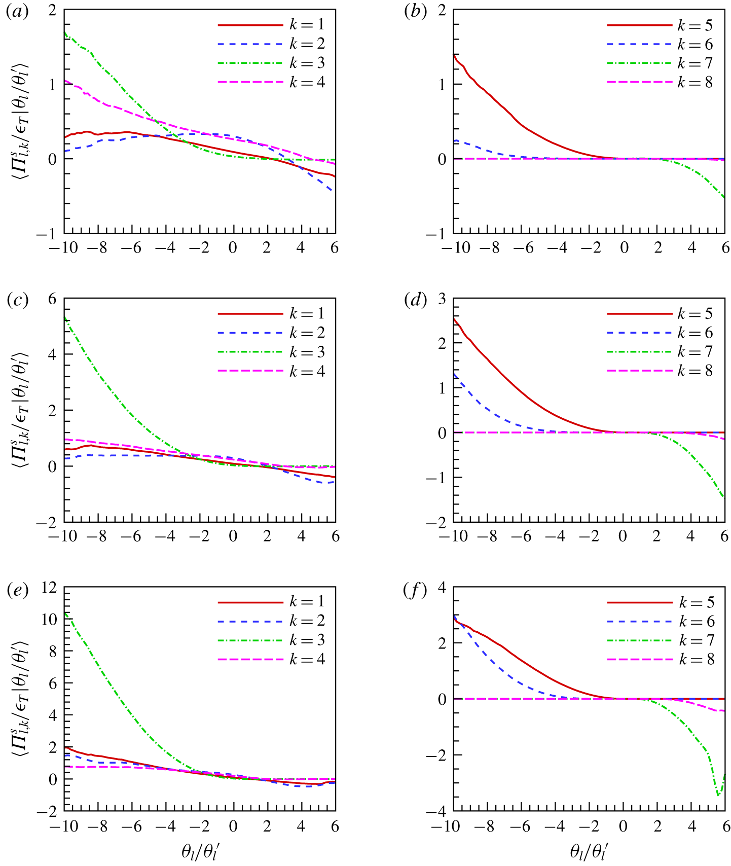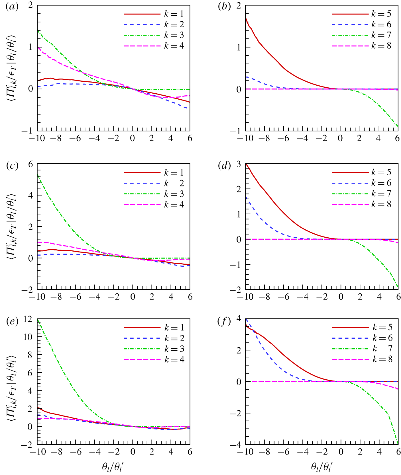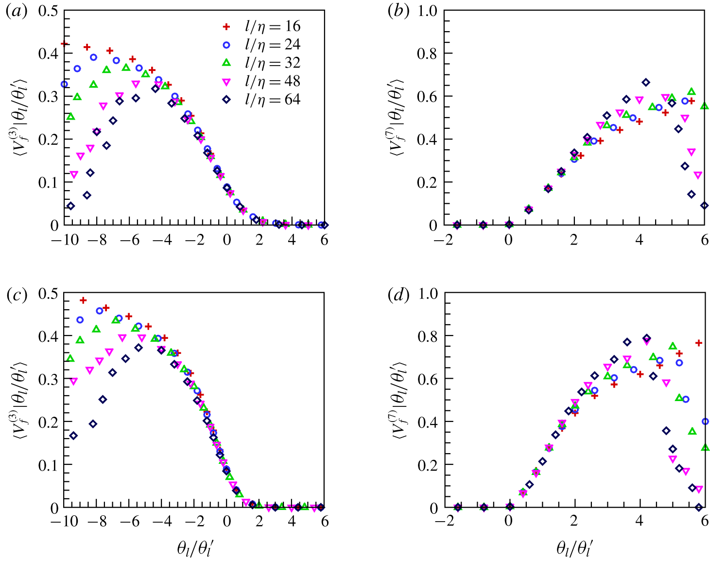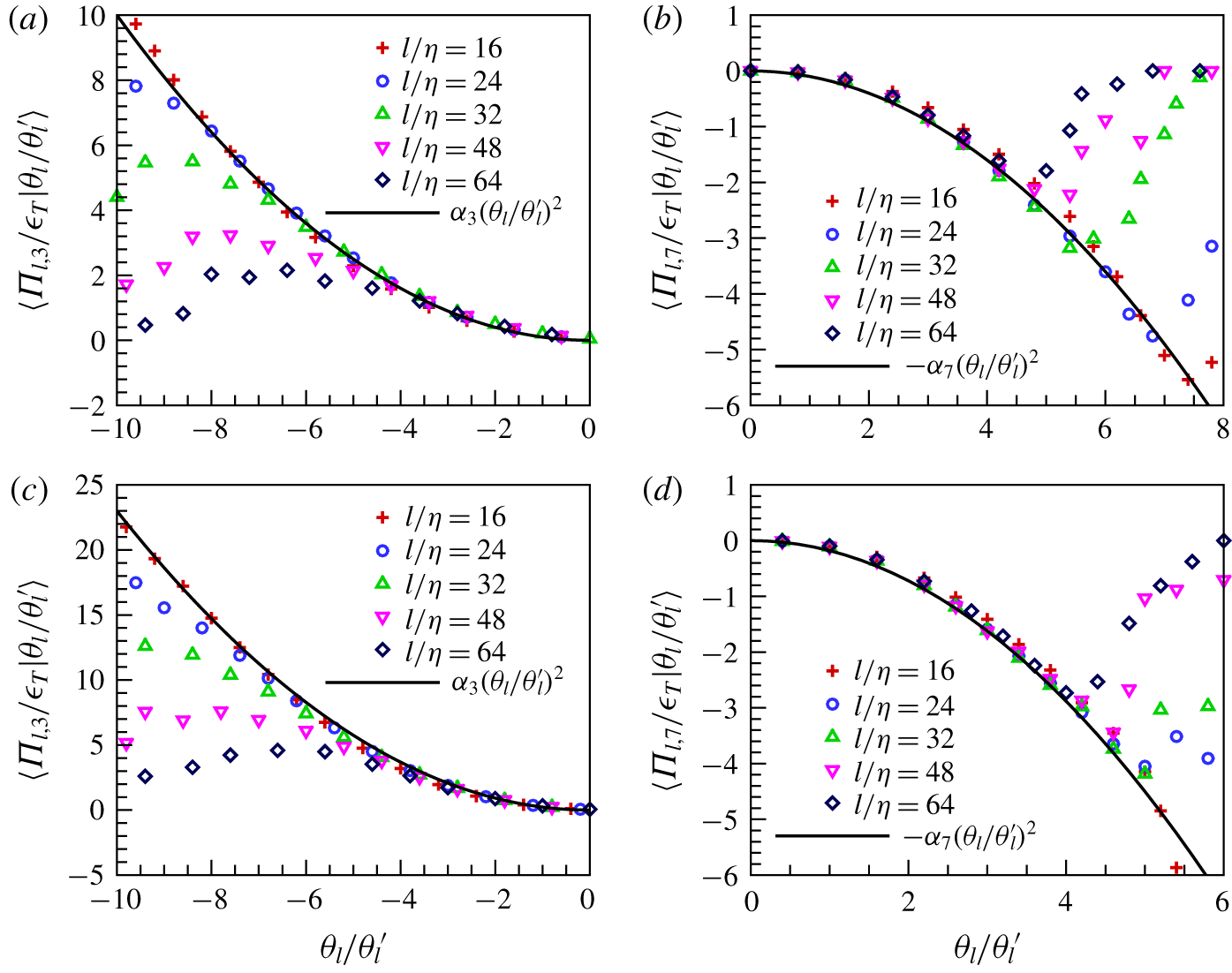
1 Introduction
Knowledge of flow topology is crucial to the understanding of various turbulence processes, including kinetic energy transfer, vortex dynamics, material element deformation and turbulent mixing. Continuous efforts have been devoted over the years to addressing the statistics and structures of the velocity gradient tensor and local flow topology in incompressible turbulence (Meneveau Reference Meneveau2011). In the pioneering work by Chong, Perry & Cantwell (Reference Chong, Perry and Cantwell1990), a general topological classification of three-dimensional flow pattern was proposed based on the three invariants of the velocity gradient tensor. A universal teardrop shape of the joint probability density function (PDF) of the second and third invariants of the velocity gradient tensor was identified in different types of incompressible turbulence, including time-developing mixing layers (Soria et al. Reference Soria, Sondergaard, Cantwell, Chong and Perry1994), turbulent channel flow (Blackburn, Mansour & Cantwell Reference Blackburn, Mansour and Cantwell1996), turbulent boundary layers (Chong et al. Reference Chong, Soria, Perry, Chacin, Cantwell and Na1998; Chacin & Cantwell Reference Chacin and Cantwell2000), isotropic turbulence (Ooi et al. Reference Ooi, Martin, Soria and Chong1999; Elsinga & Marusic Reference Elsinga and Marusic2010), homogeneous sheared turbulence (Nomura & Diamessis Reference Nomura and Diamessis2000), turbulent plane jets (Da Silva & Pereira Reference da Silva and Pereira2008) and single-square grid-generated turbulence (Zhou et al. Reference Zhou, Nagata, Sakai, Ito and Hayase2015). It was shown that local flow topology has important effects on various properties of turbulence, including turbulent kinetic energy and dissipation in the turbulent boundary layer (Chacin & Cantwell Reference Chacin and Cantwell2000), interaction of the vorticity and rate-of-strain tensor in homogeneous sheared turbulence (Nomura & Diamessis Reference Nomura and Diamessis2000), the entrainment in a turbulent jet (Da Silva & Pereira Reference da Silva and Pereira2008), the dynamics of streamlines and vortex lines (Boschung et al. Reference Boschung, Schaefer, Peters and Meneveau2014) and the stability of local flows undergoing strain, rotation, convergence, divergence and swirl (Mishra & Girimaji Reference Mishra and Girimaji2015).
It is worth noting that the velocity gradient tensor is mainly related to the turbulence dynamics near the Kolmogorov length scale. The coarse-grained or filtered velocity gradient tensor can be used to study the flow topology at larger scales of turbulence (Borue & Orszag Reference Borue and Orszag1998; Chertkov, Pumir & Shraiman Reference Chertkov, Pumir and Shraiman1999; Meneveau Reference Meneveau2011). It was found that the joint PDF of the second and third invariants of the filtered velocity gradient tensor exhibit the teardrop shape at scales of the inertial range in incompressible turbulence (Borue & Orszag Reference Borue and Orszag1998; van der Bos et al. Reference van der Bos, Tao, Meneveau and Katz2002; Lüthi et al. Reference Lüthi, Ott, Berg and Mann2007). Some phenomenological models of turbulent fluctuations revealed that the joint PDF becomes increasingly symmetric as the filter width increases (Chertkov et al. Reference Chertkov, Pumir and Shraiman1999; Naso & Pumir Reference Naso and Pumir2005; Naso, Chertkov & Pumir Reference Naso, Chertkov and Pumir2006; Naso, Pumir & Chertkov Reference Naso, Pumir and Chertkov2007; Pumir & Naso Reference Pumir and Naso2010; Johnson & Meneveau Reference Johnson and Meneveau2017). Recently, Lozano-Durán, Holzner & Jiménez (Reference Lozano-Durán, Holzner and Jiménez2016) studied the invariants of the filtered velocity gradient tensor in incompressible turbulent channel flow. They showed that the dynamics of the flow is not self-similar in the inertial range due to the effect of the mean shear. However, the self-similarity of inertial range dynamics was identified for the filtered gradient tensor of the fluctuating velocity field. Danish & Meneveau (Reference Danish and Meneveau2018) investigated the statistics of the filtered velocity gradient tensor and the population fractions of various flow topologies of the filtered field in incompressible isotropic turbulence. They observed the well-known teardrop shape of the joint PDF of the second and third invariants of the filtered velocity gradient tensor. They further addressed the different mechanisms for the evolution of the joint PDF at various scales, and pointed out that different approaches are required to model the dynamics of the filtered velocity gradient in the inertial range and in the viscous range.
The flow structures and statistical features of compressible turbulence are more complex than those of incompressible turbulence, due to the nonlinear couplings of the solenoidal mode, compressible mode and thermodynamic mode in compressible turbulence (Samtaney, Pullin & Kosovic Reference Samtaney, Pullin and Kosovic2001; Pirozzoli & Grasso Reference Pirozzoli and Grasso2004; Aluie Reference Aluie2011; Ryu & Livescu Reference Ryu and Livescu2014; Danish, Sinha & Srinivasan Reference Danish, Sinha and Srinivasan2016a; Jagannathan & Donzis Reference Jagannathan and Donzis2016; Quadros, Sinha & Larsson Reference Quadros, Sinha and Larsson2016; Yang et al. Reference Yang, Wang, Shi, Xiao, He and Chen2016; Dai et al. Reference Dai, Luo, Jin and Fan2017; Pan & Johnsen Reference Pan and Johnsen2017; Parashar et al. Reference Parashar, Sinha, Danish and Srinivasan2017; Sciacovelli, Cinnella & Grasso Reference Sciacovelli, Cinnella and Grasso2017; Wang, Gotoh & Watanabe Reference Wang, Gotoh and Watanabe2017a; Wang et al. Reference Wang, Wan, Chen and Chen2018a, Reference Wang, Wan, Chen, Xie, Wang and Chen2019). The local flow-field topology based on the three invariants of velocity gradient tensor was investigated in a wide range of compressible turbulence, including decaying compressible isotropic turbulence (Suman & Girimaji Reference Suman and Girimaji2010; Danish, Suman & Girimaji Reference Danish, Suman and Girimaji2016b), compressible turbulent boundary layers (Wang & Lu Reference Wang and Lu2012; Chu & Lu Reference Chu and Lu2013; Bechlars & Sandberg Reference Bechlars and Sandberg2017a,Reference Bechlars and Sandbergb), compressible turbulent mixing layers (Vaghefi & Madnia Reference Vaghefi and Madnia2015; Mathew, Ghosh & Friedrich Reference Mathew, Ghosh and Friedrich2016), supersonic turbulent pipes, nozzle and diffuser flows (Kumari et al. Reference Kumari, Mahapatra, Ghosh and Mathew2018) and compressible turbulent flames (Cifuentes et al. Reference Cifuentes, Dopazo, Martin and Jimenez2014, Reference Cifuentes, Dopazo, Martin, Domingo and Vervisch2016; Wacks & Chakraborty Reference Wacks and Chakraborty2016a; Wacks, Chakraborty & Klein Reference Wacks, Chakraborty and Klein2016b; Papapostolou et al. Reference Papapostolou, Wacks, Chakraborty, Klein and Im2017; Lai, Wacks & Chakraborty Reference Lai, Wacks and Chakraborty2018; Wacks, Konstantinou & Chakraborty Reference Wacks, Konstantinou and Chakraborty2018). The teardrop shape of the joint PDF of the second and third invariants of the velocity gradient tensor was identified in locally nearly incompressible regions of compressible turbulence. It was also found that the joint PDF of the second and third invariants of the anisotropic part of the velocity gradient tensor exhibits a similar teardrop shape in compressible isotropic turbulence (Pirozzoli & Grasso Reference Pirozzoli and Grasso2004; Wang et al. Reference Wang, Shi, Wang, Xiao, He and Chen2012; Sciacovelli et al. Reference Sciacovelli, Cinnella and Grasso2017). To our knowledge, a relevant study of the flow topology of the filtered velocity gradient at scales in the inertial range of compressible turbulence has never been performed.
The filtering method is an effective and convenient approach to understanding the multi-scale properties of turbulence. The filtered velocity field is used in large eddy simulation (LES) to reduce the effective degrees of freedom of the flow system and to isolate the dynamics of fluid turbulence above the filter width. The effect of small-scale flow structures on the large-scale flow dynamics is modelled by the subgrid-scale (SGS) stress in the dynamical equation of the filtered velocity. The filtering method has also been widely applied to study inter-scale transfer of kinetic energy in turbulence, revealing various spatial structures and statistical features of the SGS flux of kinetic energy (Eyink Reference Eyink2005; Aluie & Eyink Reference Aluie and Eyink2009; Eyink & Aluie Reference Eyink and Aluie2009; Aluie Reference Aluie2011; Wang et al. Reference Wang, Yang, Shi, Xiao, He and Chen2013, Reference Wang, Wan, Chen and Chen2018a). Eyink (Reference Eyink2005) proposed a smooth filtering approach to resolve the turbulent flows both in space and in scale. He theoretically established sufficient conditions for locality of the energy cascade in incompressible turbulence by an exact analysis of the filtered flow equations. The localness of the energy cascade in three-dimensional incompressible turbulence was further demonstrated by both smooth and sharp spectral filters, and verified by direct numerical simulations (Aluie & Eyink Reference Aluie and Eyink2009; Eyink & Aluie Reference Eyink and Aluie2009). Aluie (Reference Aluie2011, Reference Aluie2013) applied the filtering approach to prove that inter-scale transfer of kinetic energy in compressible turbulence is dominated by local interactions, under the assumption that the pressure-dilatation cospectrum decays at a sufficiently rapid rate. Aluie, Li & Li (Reference Aluie, Li and Li2012) further verified the result by numerical simulations of both forced and decaying compressible isotropic turbulence. Wang et al. (Reference Wang, Yang, Shi, Xiao, He and Chen2013) performed numerical simulations of compressible isotropic turbulence by applying a large-scale force to both the solenoidal and compressible components of the velocity field. They found that the SGS kinetic energy flux is dominated by the compressible mode of the velocity in the inertial range, due to the effect of large-scale shock waves in the simulated flow. Wang et al. (Reference Wang, Wan, Chen and Chen2018a) studied the kinetic energy transfer in compressible isotropic turbulence by numerical simulations with solenoidal forcing. They applied the filtering method to show that with the increase of the turbulent Mach number, compression motions enhance the positive SGS flux of kinetic energy, and expansion motions enhance the negative SGS flux of kinetic energy. They found that the compressible mode persistently absorbs kinetic energy from the solenoidal mode through nonlinear advection. Moreover, the kinetic energy of compressible mode cascades from large scales to small scales through the compressible SGS flux, and is dissipated by viscosity at small scales. Aluie (Reference Aluie2013) pointed out that the sharp spectral filter is not positive in physical space, and a filtered density using the sharp spectral filter can have negative values in space, which would violate fundamental conservation laws. Different from the sharp spectral filter, the top-hat filter and the Gaussian filter are positive in physical space, and can be interpreted as a local spatial average. Wang et al. (Reference Wang, Wan, Chen and Chen2018a) showed that the behaviours of kinetic energy transfer using the top-hat filter are similar to those using the Gaussian filter, and are consistent with the theoretical analysis by Aluie (Reference Aluie2013).
In large eddy simulation of turbulence, the SGS stress is usually reconstructed from the filtered velocity gradient, giving rise to a variety of eddy-viscosity models and algebraic models (Meneveau & Katz Reference Meneveau and Katz2000). Thus, study of the filtered velocity gradient is of direct importance to the physical understanding of kinetic energy transfer and development of SGS models. Recently, machine learning has frequently been used to help develop more accurate turbulence models, but this does not usually help with physical interpretation (Duraisamy, Iaccarino & Xiao Reference Duraisamy, Iaccarino and Xiao2019). It was shown that embedding more invariance properties into turbulence models does indeed improve the resulting models for closure terms in the Reynolds-averaged turbulence statistics (Ling, Jones & Templeton Reference Ling, Jones and Templeton2016a; Ling, Kurzawski & Templeton Reference Ling, Kurzawski and Templeton2016b). Moreover, an artificial neural network was applied to develop SGS stress models from the filtered velocity gradient for large eddy simulation of turbulence (Gamahara & Hattori Reference Gamahara and Hattori2017; Wang et al. Reference Wang, Luo, Li, Tan and Fan2018; Xie et al. Reference Xie, Wang, Li and Ma2019). In the development of the SGS models, each component of SGS stress was trained separately, and the invariance properties and physical realizability of the SGS stress were not considered. We believe that knowledge of the invariance properties of the filtered velocity gradient is crucial to developing more accurate and efficient SGS stress models. The flow topology derived from invariance properties is expected to be directly related to the local spatial structure of the filtered velocity and can play an important role in the development of LES models.
In this study, we investigate the flow topology of the filtered velocity gradient and its impact on kinetic energy flux in solenoidally forced compressible isotropic turbulence at turbulent Mach numbers ranging from 0.6 to 1.0 and at a Taylor Reynolds number of approximately 250. The rest of the paper is organized as follows. The governing equations and numerical method are provided in § 2. The simulation parameters and one-point statistics of the simulated flow are shown in § 3. A filtering approach is introduced to perform a multiscale analysis of turbulence in § 4. Definitions of flow topologies based on the three invariants of the filtered velocity gradient tensor are given in § 5. Numerical results for the effect of flow topology on the kinetic energy flux in compressible isotropic turbulence are presented in § 6. Main conclusions are summarized in § 7.
2 Governing equations and numerical method
We study compressible isotropic turbulence of an ideal gas governed by the following dimensionless Navier–Stokes equations in the conservative form (Samtaney et al. Reference Samtaney, Pullin and Kosovic2001; Wang et al. Reference Wang, Wan, Chen and Chen2018a,Reference Wang, Wan, Chen, Xie and Chenb):
 $$\begin{eqnarray}\displaystyle & \displaystyle \frac{\unicode[STIX]{x2202}\unicode[STIX]{x1D70C}}{\unicode[STIX]{x2202}t}+\frac{\unicode[STIX]{x2202}(\unicode[STIX]{x1D70C}u_{j})}{\unicode[STIX]{x2202}x_{j}}=0, & \displaystyle\end{eqnarray}$$
 $$\begin{eqnarray}\displaystyle & \displaystyle \frac{\unicode[STIX]{x2202}(\unicode[STIX]{x1D70C}u_{i})}{\unicode[STIX]{x2202}t}+\frac{\unicode[STIX]{x2202}[\unicode[STIX]{x1D70C}u_{i}u_{j}+p\unicode[STIX]{x1D6FF}_{ij}]}{\unicode[STIX]{x2202}x_{j}}=\frac{1}{Re_{r}}\frac{\unicode[STIX]{x2202}\unicode[STIX]{x1D70E}_{ij}}{\unicode[STIX]{x2202}x_{j}}+{\mathcal{F}}_{i}, & \displaystyle\end{eqnarray}$$
 $$\begin{eqnarray}\displaystyle & \displaystyle \frac{\unicode[STIX]{x2202}{\mathcal{E}}}{\unicode[STIX]{x2202}t}+\frac{\unicode[STIX]{x2202}[({\mathcal{E}}+p)u_{j}]}{\unicode[STIX]{x2202}x_{j}}=\frac{1}{\unicode[STIX]{x1D6FC}}\frac{\unicode[STIX]{x2202}}{\unicode[STIX]{x2202}x_{j}}\left(\unicode[STIX]{x1D705}\frac{\unicode[STIX]{x2202}T}{\unicode[STIX]{x2202}x_{j}}\right)+\frac{1}{Re_{r}}\frac{\unicode[STIX]{x2202}(\unicode[STIX]{x1D70E}_{ij}u_{i})}{\unicode[STIX]{x2202}x_{j}}-\unicode[STIX]{x1D6EC}+{\mathcal{F}}_{j}u_{j}, & \displaystyle\end{eqnarray}$$
 $$\begin{eqnarray}\displaystyle & \displaystyle p=\unicode[STIX]{x1D70C}T/(\unicode[STIX]{x1D6FE}M_{r}^{2}), & \displaystyle\end{eqnarray}$$
where  $u_{i}$,
 $\unicode[STIX]{x1D70C}$,
 $p$ and
 $T$ are the velocity component, density, pressure and temperature, respectively. Here,
 ${\mathcal{E}}$ is the total energy per unit volume, which is given by
 $$\begin{eqnarray}{\mathcal{E}}=\frac{p}{\unicode[STIX]{x1D6FE}-1}+\frac{1}{2}\unicode[STIX]{x1D70C}(u_{j}u_{j}).\end{eqnarray}$$
The viscous stress  $\unicode[STIX]{x1D70E}_{ij}$ is defined by
 $$\begin{eqnarray}\unicode[STIX]{x1D70E}_{ij}=\unicode[STIX]{x1D707}\left(\frac{\unicode[STIX]{x2202}u_{i}}{\unicode[STIX]{x2202}x_{j}}+\frac{\unicode[STIX]{x2202}u_{j}}{\unicode[STIX]{x2202}x_{i}}\right)-\frac{2}{3}\unicode[STIX]{x1D707}\unicode[STIX]{x1D703}\unicode[STIX]{x1D6FF}_{ij},\end{eqnarray}$$
where  $\unicode[STIX]{x1D703}=\unicode[STIX]{x2202}u_{k}/\unicode[STIX]{x2202}x_{k}$ is the velocity divergence. Moreover,
 ${\mathcal{F}}_{i}$ is a large-scale forcing, and
 $\unicode[STIX]{x1D6EC}$ is a large-scale cooling function.
The variables in the governing equations of compressible turbulence have been already normalized by a set of reference scales, including the reference length  $L_{r}$, velocity
 $U_{r}$, density
 $\unicode[STIX]{x1D70C}_{r}$, pressure
 $p_{r}=\unicode[STIX]{x1D70C}_{r}U_{r}^{2}$, temperature
 $T_{r}$, energy per unit volume
 $\unicode[STIX]{x1D70C}_{r}U_{r}^{2}$, viscosity
 $\unicode[STIX]{x1D707}_{r}$ and thermal conductivity
 $\unicode[STIX]{x1D705}_{r}$ (Samtaney et al. Reference Samtaney, Pullin and Kosovic2001; Wang et al. Reference Wang, Wang, Xiao, Shi and Chen2010, Reference Wang, Wan, Chen and Chen2018a,Reference Wang, Wan, Chen, Xie and Chenb). The reference speed of sound is defined by
 $c_{r}=\sqrt{\unicode[STIX]{x1D6FE}RT_{r}}$, where
 $R$ is the specific gas constant;
 $\unicode[STIX]{x1D6FE}=C_{p}/C_{v}$ is the ratio of specific heat at constant pressure
 $C_{p}$ to that at constant volume
 $C_{v}$. It is assumed that
 $\unicode[STIX]{x1D6FE}=1.4$. There are three reference governing parameters: the reference Reynolds number
 $Re_{r}=\unicode[STIX]{x1D70C}_{r}U_{r}L_{r}/\unicode[STIX]{x1D707}_{r}$, the reference Mach number
 $M_{r}=U_{r}/c_{r}$ and the reference Prandtl number
 $Pr=\unicode[STIX]{x1D707}_{r}C_{p}/\unicode[STIX]{x1D705}_{r}$. It is assumed that
 $Pr=0.7$. The parameter
 $\unicode[STIX]{x1D6FC}$ is given by
 $\unicode[STIX]{x1D6FC}=Pr\,Re_{r}(\unicode[STIX]{x1D6FE}-1)M_{r}^{2}$. The Prandtl number
 $Pr$ signifies the relative importance of momentum diffusivity and thermal diffusivity: a small value of the Prandtl number indicates that the thermal diffusivity predominates over momentum diffusivity, where the fluctuations of temperature are suppressed; in contrast, in the situation of large Prandtl number, the fluctuations of temperature are enhanced.
We solve the governing equations of compressible isotropic turbulence numerically in a cubic box with side lengths  $2\unicode[STIX]{x03C0}$, using a uniform grid with
 $1024^{3}$ grid points. Periodic boundary conditions are employed in all three spatial directions. We apply a hybrid compact-weighted essentially non-oscillatory (WENO) scheme (Wang et al. Reference Wang, Wang, Xiao, Shi and Chen2010), which combines an eighth-order compact finite difference scheme (Lele Reference Lele1992) in smooth regions and a seventh-order WENO scheme (Balsara & Shu Reference Balsara and Shu2000) in shock regions. The numerical simulations essentially resolve flow fields above the Kolmogorov length scale, while the discontinuities around shock waves are captured by the WENO scheme. Grid-refinement convergence studies of compressible isotropic turbulence for the convergence of small-scale statistics have been performed at turbulent Mach number
 $M_{t}=1.0$ previously (Wang et al. Reference Wang, Shi, Wang, Xiao, He and Chen2011, Reference Wang, Shi, Wang, Xiao, He and Chen2012).
We use Sutherland’s law to obtain the non-dimensional temperature-dependent viscosity coefficient  $\unicode[STIX]{x1D707}$ and thermal conductivity coefficient
 $\unicode[STIX]{x1D705}$ (Wang et al. Reference Wang, Wang, Xiao, Shi and Chen2010):
 $$\begin{eqnarray}\displaystyle & \displaystyle \unicode[STIX]{x1D707}=\frac{1.4042T^{1.5}}{T+0.40417}, & \displaystyle\end{eqnarray}$$
 $$\begin{eqnarray}\displaystyle & \displaystyle \unicode[STIX]{x1D705}=\frac{1.4042T^{1.5}}{T+0.40417}. & \displaystyle\end{eqnarray}$$
It has been shown that Sutherland’s law for the viscosity coefficient of air has a maximum relative error of  $2.0\,\%$ at
 $T=3$ and less than
 $0.52\,\%$ at
 $T=0.55$ as compared to the measured viscosity data, with reference dimensional viscosity
 $\unicode[STIX]{x1D707}_{r}=1.716\times 10^{-5}~\text{kg}~(\text{m}~\text{s})^{-1}$ at the reference temperature of
 $T_{r}=273.15~\text{K}$ (Wang et al. Reference Wang, Wang, Xiao, Shi and Chen2010).
The velocity field is forced by fixing the energy spectrum within the two lowest wavenumber shells (Wang et al. Reference Wang, Wang, Xiao, Shi and Chen2010). The force is only applied to the solenoidal component of the velocity field. The internal energy is sustained in a statistically steady state by a spatially uniform thermal cooling  $\unicode[STIX]{x1D6EC}$. Similar to the situation of incompressible isotropic turbulence, the forcing field is constructed in Fourier space, which is performed as follows (Wang et al. Reference Wang, Wang, Xiao, Shi and Chen2010). The velocity field
 $\boldsymbol{u}(\boldsymbol{x},t)$ is first transformed into Fourier space to yield
 $\hat{\boldsymbol{u}}(\boldsymbol{k},t)$, where
 $\boldsymbol{k}$ represents wave vector in Fourier space. Then,
 $\hat{\boldsymbol{u}}(\boldsymbol{k},t)$ is decomposed into a solenoidal component
 $\hat{\boldsymbol{u}}^{s}(\boldsymbol{k},t)$ and a compressible component
 $\hat{\boldsymbol{u}}^{c}(\boldsymbol{k},t)$,
 $$\begin{eqnarray}\hat{\boldsymbol{u}}(\boldsymbol{k},t)=\hat{\boldsymbol{u}}^{s}(\boldsymbol{k},t)+\hat{\boldsymbol{u}}^{c}(\boldsymbol{k},t),\end{eqnarray}$$
where
 $$\begin{eqnarray}\displaystyle & \displaystyle \hat{\boldsymbol{u}}^{s}(\boldsymbol{k},t)=\hat{\boldsymbol{u}}(\boldsymbol{k},t)-\frac{\boldsymbol{k}\boldsymbol{k}\boldsymbol{\cdot }\hat{\boldsymbol{u}}(\boldsymbol{k},t)}{k^{2}}, & \displaystyle\end{eqnarray}$$
 $$\begin{eqnarray}\displaystyle & \displaystyle \hat{\boldsymbol{u}}^{c}(\boldsymbol{k},t)=\frac{\boldsymbol{k}\boldsymbol{k}\boldsymbol{\cdot }\hat{\boldsymbol{u}}(\boldsymbol{k},t)}{k^{2}}. & \displaystyle\end{eqnarray}$$
The kinetic energy per unit mass associated with each wave vector can be decomposed in a similar manner:
 $$\begin{eqnarray}{\textstyle \frac{1}{2}}|\hat{\boldsymbol{u}}(\boldsymbol{k},t)|^{2}={\textstyle \frac{1}{2}}|\hat{\boldsymbol{u}}^{s}(\boldsymbol{k},t)|^{2}+{\textstyle \frac{1}{2}}|\hat{\boldsymbol{u}}^{c}(\boldsymbol{k},t)|^{2}.\end{eqnarray}$$
The kinetic energy in each of the first two wavenumber shells can be calculated by summing over all modes belonging to a given wavenumber shell,
 $$\begin{eqnarray}\displaystyle & \displaystyle E(0.5\leqslant k<1.5)=\mathop{\sum }_{0.5\leqslant |\boldsymbol{k}|<1.5}\left(\frac{1}{2}|\hat{\boldsymbol{u}}(\boldsymbol{k},t)|^{2}\right), & \displaystyle\end{eqnarray}$$
 $$\begin{eqnarray}\displaystyle & \displaystyle E(1.5\leqslant k<2.5)=\mathop{\sum }_{1.5\leqslant |\boldsymbol{k}|<2.5}\left(\frac{1}{2}|\hat{\boldsymbol{u}}(\boldsymbol{k},t)|^{2}\right). & \displaystyle\end{eqnarray}$$
It is straightforward to derive the following relations:
 $$\begin{eqnarray}\displaystyle & \displaystyle E(0.5\leqslant k<1.5)=E^{s}(0.5\leqslant k<1.5)+E^{c}(0.5\leqslant k<1.5), & \displaystyle\end{eqnarray}$$
 $$\begin{eqnarray}\displaystyle & \displaystyle E(1.5\leqslant k<2.5)=E^{s}(1.5\leqslant k<2.5)+E^{c}(1.5\leqslant k<2.5). & \displaystyle\end{eqnarray}$$
The force is constructed by amplifying the solenoidal component of the velocity field, to maintain the total kinetic energy in the first two shells to prescribed levels  $E_{0}(1)$ and
 $E_{0}(2)$, respectively. The forced velocity
 $\hat{\boldsymbol{u}}^{f}(\boldsymbol{k},t)$ is given by
 $$\begin{eqnarray}\hat{\boldsymbol{u}}^{f}(\boldsymbol{k},t)=\unicode[STIX]{x1D6FD}_{f}\hat{\boldsymbol{u}}^{s}(\boldsymbol{k},t)+\hat{\boldsymbol{u}}^{c}(\boldsymbol{k},t),\end{eqnarray}$$
where
 $$\begin{eqnarray}\displaystyle & \displaystyle \unicode[STIX]{x1D6FD}_{f}(0.5\leqslant k<1.5)=\sqrt{\frac{E_{0}(1)-E^{c}(0.5\leqslant k<1.5)}{E^{s}(0.5\leqslant k<1.5)}}, & \displaystyle\end{eqnarray}$$
 $$\begin{eqnarray}\displaystyle & \displaystyle \unicode[STIX]{x1D6FD}_{f}(1.5\leqslant k<2.5)=\sqrt{\frac{E_{0}(2)-E^{c}(1.5\leqslant k<2.5)}{E^{s}(1.5\leqslant k<2.5)}}. & \displaystyle\end{eqnarray}$$
Typically,  $E_{0}(1)=1.242477$ and
 $E_{0}(2)=0.391356$ are used in the numerical simulation. There are several previous studies on solenoidally forced compressible isotropic turbulence at turbulent Mach numbers up to
 $1.0$, revealing that the overall statistical properties of the solenoidal velocity component are similar to those of the velocity field in incompressible isotropic turbulence, including the spectrum and the structure function of the solenoidal velocity and the statistics of vorticity (Wang et al. Reference Wang, Shi, Wang, Xiao, He and Chen2011, Reference Wang, Shi, Wang, Xiao, He and Chen2012, Reference Wang, Gotoh and Watanabe2017a; Wang, Gotoh & Watanabe Reference Wang, Gotoh and Watanabe2017c). It was also shown that the ratio of compressible kinetic energy to its solenoidal counterpart is always smaller than
 $5\,\%$ (Wang et al. Reference Wang, Gotoh and Watanabe2017a). Moreover, the compressible mode persistently absorbs kinetic energy from the solenoidal mode through nonlinear advection, and exhibits energy cascade from large scales to small scales through the compressible SGS flux (Wang et al. Reference Wang, Wan, Chen and Chen2018a).
Simulation parameters and flow statistics.

3 Simulation parameters and one-point statistics
One-point statistics for three simulated compressible isotropic turbulent flows are summarized in table 1. The Taylor microscale Reynolds number  $Re_{\unicode[STIX]{x1D706}}$ is given by (Wang et al. Reference Wang, Shi, Wang, Xiao, He and Chen2012)
 $$\begin{eqnarray}Re_{\unicode[STIX]{x1D706}}=\frac{(\unicode[STIX]{x1D70C}_{r}\langle \unicode[STIX]{x1D70C}\rangle )(U_{r}u^{\prime }/\sqrt{3})(L_{r}\unicode[STIX]{x1D706})}{(\unicode[STIX]{x1D707}_{r}\langle \unicode[STIX]{x1D707}\rangle )}=Re_{r}\frac{\langle \unicode[STIX]{x1D70C}\rangle u^{\prime }\unicode[STIX]{x1D706}}{\sqrt{3}\langle \unicode[STIX]{x1D707}\rangle },\end{eqnarray}$$
where  $\langle \rangle$ stands for spatial average and the reference Reynolds number
 $Re_{r}=\unicode[STIX]{x1D70C}_{r}U_{r}L_{r}/\unicode[STIX]{x1D707}_{r}$. The root mean square (r.m.s.) value of the velocity magnitude is defined as
 $u^{\prime }=\sqrt{\langle u_{1}^{2}+u_{2}^{2}+u_{3}^{2}\rangle }$, and the Taylor microscale is calculated by
 $$\begin{eqnarray}\unicode[STIX]{x1D706}=\sqrt{\frac{\langle u_{1}^{2}+u_{2}^{2}+u_{3}^{2}\rangle }{\langle (\unicode[STIX]{x2202}u_{1}/\unicode[STIX]{x2202}x_{1})^{2}+(\unicode[STIX]{x2202}u_{2}/\unicode[STIX]{x2202}x_{2})^{2}+(\unicode[STIX]{x2202}u_{3}/\unicode[STIX]{x2202}x_{3})^{2}\rangle }}.\end{eqnarray}$$
The Taylor microscale Reynolds number is close to  $250$ in our numerical simulations. The turbulent Mach number
 $M_{t}$ is defined by
 $$\begin{eqnarray}M_{t}=\frac{(U_{r}u^{\prime })}{\langle \sqrt{\unicode[STIX]{x1D6FE}R(T_{r}T)}\rangle }=M_{r}\frac{u^{\prime }}{\langle \sqrt{T}\rangle },\end{eqnarray}$$
where the reference Mach number  $M_{r}=U_{r}/c_{r}$. Three different turbulent Mach numbers are considered:
 $0.6$,
 $0.8$ and
 $1.0$, corresponding to the different levels of compressibility.
The Kolmogorov length scale  $\unicode[STIX]{x1D702}$ is defined by
 $\unicode[STIX]{x1D702}=[\langle \unicode[STIX]{x1D707}/(Re_{r}\unicode[STIX]{x1D70C})\rangle ^{3}/\unicode[STIX]{x1D716}]^{1/4}$, where
 $\unicode[STIX]{x1D716}$ is the spatial average of the dissipation rate of kinetic energy per unit mass:
 $\unicode[STIX]{x1D716}=\langle \unicode[STIX]{x1D70E}_{ij}\unicode[STIX]{x1D61A}_{ij}/(Re_{r}\unicode[STIX]{x1D70C})\rangle$. Here, the strain-rate tensor
 $\unicode[STIX]{x1D61A}_{ij}$ is given by
 $\unicode[STIX]{x1D61A}_{ij}=(\unicode[STIX]{x2202}u_{i}/\unicode[STIX]{x2202}x_{j}+\unicode[STIX]{x2202}u_{j}/\unicode[STIX]{x2202}x_{i})/2$. It is shown that the resolution parameter
 $\unicode[STIX]{x1D702}/\unicode[STIX]{x0394}x$ is in the range
 $1.02\leqslant \unicode[STIX]{x1D702}/\unicode[STIX]{x0394}x\leqslant 1.05$, where
 $\unicode[STIX]{x0394}x$ is the grid length in each direction. Consequently, the resolution parameter
 $k_{max}\unicode[STIX]{x1D702}$ is in the range
 $3.2\leqslant k_{max}\unicode[STIX]{x1D702}\leqslant 3.3$, where the largest wavenumber
 $k_{max}$ is half of the number of grids
 $N$ in each direction:
 $k_{max}=N/2=\unicode[STIX]{x03C0}/\unicode[STIX]{x0394}x$. Previous grid-refinement convergence studies of compressible isotropic turbulence at turbulent Mach number
 $M_{t}=1.0$ (Wang et al. Reference Wang, Shi, Wang, Xiao, He and Chen2011, Reference Wang, Shi, Wang, Xiao, He and Chen2012) showed that resolutions of
 $k_{max}\geqslant 3.2$ are enough for the convergence of small-scale statistics, including the kinetic energy spectrum at different wavenumbers and the PDFs of the velocity divergence and vorticity.
The integral length scale  $L_{I}$ is calculated by (Wang et al. Reference Wang, Shi, Wang, Xiao, He and Chen2012)
 $$\begin{eqnarray}L_{I}=\frac{3\unicode[STIX]{x03C0}}{2(u^{\prime })^{2}}\int _{0}^{\infty }\frac{E(k)}{k}\,\text{d}k,\end{eqnarray}$$
where  $E(k)$ is the spectrum of kinetic energy per unit mass, namely,
 $\int _{0}^{\infty }E(k)\,\text{d}k=(u^{\prime })^{2}/2$. It is found that
 $226\leqslant L_{I}/\unicode[STIX]{x1D702}\leqslant 231$ in the numerical simulations.
The velocity derivative skewness  $S_{3}$ is defined by
 $$\begin{eqnarray}S_{3}=\frac{[\langle (\unicode[STIX]{x2202}u_{1}/\unicode[STIX]{x2202}x_{1})^{3}+(\unicode[STIX]{x2202}u_{2}/\unicode[STIX]{x2202}x_{2})^{3}+(\unicode[STIX]{x2202}u_{3}/\unicode[STIX]{x2202}x_{3})^{3}\rangle ]/3}{\{\langle (\unicode[STIX]{x2202}u_{1}/\unicode[STIX]{x2202}x_{1})^{2}+(\unicode[STIX]{x2202}u_{2}/\unicode[STIX]{x2202}x_{2})^{2}+(\unicode[STIX]{x2202}u_{3}/\unicode[STIX]{x2202}x_{3})^{2}\rangle /3\}^{3/2}}.\end{eqnarray}$$
It is shown that  $S_{3}=-0.53$ at
 $M_{t}=0.6$, which is close to typical values of
 $-0.6$ to
 $-0.4$ in incompressible turbulence (Ishihara et al. Reference Ishihara, Kaneda, Yokokawa, Itakura and Uno2007). Due to the effect of shocklets, the magnitude of
 $S_{3}$ increases as the turbulent Mach number becomes larger, for
 $M_{t}=0.8$ and
 $M_{t}=1.0$ (Wang et al. Reference Wang, Shi, Wang, Xiao, He and Chen2011; Wang, Gotoh & Watanabe Reference Wang, Gotoh and Watanabe2017b; Wang et al. Reference Wang, Gotoh and Watanabe2017c).
The r.m.s. value of vorticity  $\unicode[STIX]{x1D74E}=\unicode[STIX]{x1D735}\times \boldsymbol{u}$ is calculated by
 $\unicode[STIX]{x1D714}^{\prime }=\sqrt{\langle \unicode[STIX]{x1D714}_{1}^{2}+\unicode[STIX]{x1D714}_{2}^{2}+\unicode[STIX]{x1D714}_{3}^{2}\rangle }$. The r.m.s. values of velocity divergence and strain-rate tensor are obtained by
 $\unicode[STIX]{x1D703}^{\prime }=\sqrt{\langle \unicode[STIX]{x1D703}^{2}\rangle }$ and
 $S^{\prime }=\sqrt{\langle \unicode[STIX]{x1D61A}_{ij}\unicode[STIX]{x1D61A}_{ij}\rangle }$, respectively. It is found that
 $\unicode[STIX]{x1D714}^{\prime }$ is insensitive to the change of turbulent Mach number. Due to the significant effect of compressibility,
 $\unicode[STIX]{x1D703}^{\prime }$ increases rapidly with the increase of
 $M_{t}$ (Jagannathan & Donzis Reference Jagannathan and Donzis2016; Wang et al. Reference Wang, Gotoh and Watanabe2017b,Reference Wang, Gotoh and Watanabec). It is shown that
 $0.715\leqslant S^{\prime }/\unicode[STIX]{x1D714}^{\prime }\leqslant 0.793$ in the numerical simulations, compared to 0.707 for the incompressible turbulence.
4 Multiscale analysis of turbulence by a filtering approach
A filtering technique (Martin, Piomelli & Candler Reference Martin, Piomelli and Candler2000; Meneveau & Katz Reference Meneveau and Katz2000; Aluie Reference Aluie2011; Wang et al. Reference Wang, Yang, Shi, Xiao, He and Chen2013) can be applied to perform a multiscale analysis of compressible turbulence. For a given field  $f$, a filtered field
 $\overline{f}$ is defined by
 $$\begin{eqnarray}\overline{f}(\boldsymbol{x})\equiv \int \,\text{d}^{3}\boldsymbol{r}G_{l}(\boldsymbol{r})f(\boldsymbol{x}+\boldsymbol{r}),\end{eqnarray}$$
where  $G_{l}(\boldsymbol{r})\equiv l^{-3}G(\boldsymbol{r}/l)$ is the filter function, and
 $G(\boldsymbol{r})$ is a normalized window function. Here,
 $l$ is the filter width associated with the wavelength of the smallest scale retained by the filtering operation. The Favre filtered field is defined as
 $\widetilde{f}\equiv \overline{\unicode[STIX]{x1D70C}f}/\overline{\unicode[STIX]{x1D70C}}$. A top-hat filter is used in our numerical analysis, which is calculated in one dimension by (Martin et al. Reference Martin, Piomelli and Candler2000)
 $$\begin{eqnarray}\overline{f}_{i}=\frac{1}{4n}\left(f_{i-n}+2\mathop{\sum }_{j=i-n+1}^{i+n-1}f_{j}+f_{i+n}\right),\end{eqnarray}$$
where the filter width is  $l=2n\unicode[STIX]{x0394}x$.
The filtered equation for the momentum is
 $$\begin{eqnarray}\frac{\unicode[STIX]{x2202}(\overline{\unicode[STIX]{x1D70C}}\widetilde{u}_{i})}{\unicode[STIX]{x2202}t}+\frac{\unicode[STIX]{x2202}[\overline{\unicode[STIX]{x1D70C}}\widetilde{u}_{i}\widetilde{u}_{j}+\overline{p}\unicode[STIX]{x1D6FF}_{ij}]}{\unicode[STIX]{x2202}x_{j}}=-\frac{\unicode[STIX]{x2202}(\overline{\unicode[STIX]{x1D70C}}\widetilde{\unicode[STIX]{x1D70F}}_{ij})}{\unicode[STIX]{x2202}x_{j}}+\frac{1}{Re}\frac{\unicode[STIX]{x2202}\overline{\unicode[STIX]{x1D70E}}_{ij}}{\unicode[STIX]{x2202}x_{j}},\end{eqnarray}$$
where the SGS stress is  $\overline{\unicode[STIX]{x1D70C}}\widetilde{\unicode[STIX]{x1D70F}}_{ij}=\overline{\unicode[STIX]{x1D70C}}(\widetilde{u_{i}u_{j}}-\widetilde{u}_{i}\widetilde{u}_{j})$. The appearance of the SGS stress is caused by the nonlinear effect of eliminated scales below
 $l$. The equation for the average of large-scale kinetic energy
 $\langle \overline{\unicode[STIX]{x1D70C}}\widetilde{u}_{i}^{2}/2\rangle$ can be derived as (Aluie Reference Aluie2011, Reference Aluie2013; Wang et al. Reference Wang, Yang, Shi, Xiao, He and Chen2013, Reference Wang, Wan, Chen and Chen2018a)
 $$\begin{eqnarray}\frac{\unicode[STIX]{x2202}}{\unicode[STIX]{x2202}t}\left\langle \frac{1}{2}\overline{\unicode[STIX]{x1D70C}}\widetilde{u}_{i}^{2}\right\rangle =-\langle \unicode[STIX]{x1D6F7}_{l}\rangle -\langle \unicode[STIX]{x1D6F1}_{l}\rangle -\langle D_{l}\rangle .\end{eqnarray}$$
Here,  $\unicode[STIX]{x1D6F7}_{l}$ is the large-scale pressure-dilatation term;
 $\unicode[STIX]{x1D6F1}_{l}$ is the SGS kinetic energy flux;
 $D_{l}$ is the viscous dissipation term. These terms are defined as
 $$\begin{eqnarray}\displaystyle & \displaystyle \unicode[STIX]{x1D6F7}_{l}=-\overline{p}\frac{\unicode[STIX]{x2202}\widetilde{u}_{i}}{\unicode[STIX]{x2202}x_{i}}, & \displaystyle\end{eqnarray}$$
 $$\begin{eqnarray}\displaystyle & \displaystyle \unicode[STIX]{x1D6F1}_{l}=-\overline{\unicode[STIX]{x1D70C}}\widetilde{\unicode[STIX]{x1D70F}}_{ij}\frac{\unicode[STIX]{x2202}\widetilde{u}_{i}}{\unicode[STIX]{x2202}x_{j}}=-\overline{\unicode[STIX]{x1D70C}}\widetilde{\unicode[STIX]{x1D70F}}_{ij}\widetilde{\unicode[STIX]{x1D61A}}_{ij}, & \displaystyle\end{eqnarray}$$
and
 $$\begin{eqnarray}D_{l}=\frac{\overline{\unicode[STIX]{x1D70E}}_{ij}}{Re}\frac{\unicode[STIX]{x2202}\widetilde{u}_{i}}{\unicode[STIX]{x2202}x_{j}},\end{eqnarray}$$
where the filtered strain-rate tensor  $\widetilde{\unicode[STIX]{x1D64E}}$ is defined as
 $\widetilde{\unicode[STIX]{x1D61A}}_{ij}=(\unicode[STIX]{x2202}\widetilde{u}_{i}/\unicode[STIX]{x2202}x_{j}+\unicode[STIX]{x2202}\widetilde{u}_{j}/\unicode[STIX]{x2202}x_{i})/2$.
A filtered density-weighted variable can be introduced as  $\widetilde{\boldsymbol{w}}=\sqrt{\overline{\unicode[STIX]{x1D70C}}}\widetilde{\boldsymbol{u}}$. Helmholtz decomposition on
 $\widetilde{\boldsymbol{w}}$ yields
 $\widetilde{\boldsymbol{w}}=\widetilde{\boldsymbol{w}}^{s}+\widetilde{\boldsymbol{w}}^{c}$, where
 $\widetilde{\boldsymbol{w}}^{s}$ and
 $\widetilde{\boldsymbol{w}}^{c}$ are the solenoidal and compressible components, respectively (Wang et al. Reference Wang, Yang, Shi, Xiao, He and Chen2013, Reference Wang, Wan, Chen and Chen2018a). The two components of the filtered density-weighted variable satisfy the following relations:
 $\unicode[STIX]{x1D735}\boldsymbol{\cdot }\widetilde{\boldsymbol{w}}^{s}=0$ and
 $\unicode[STIX]{x1D735}\times \widetilde{\boldsymbol{w}}^{c}=0$.
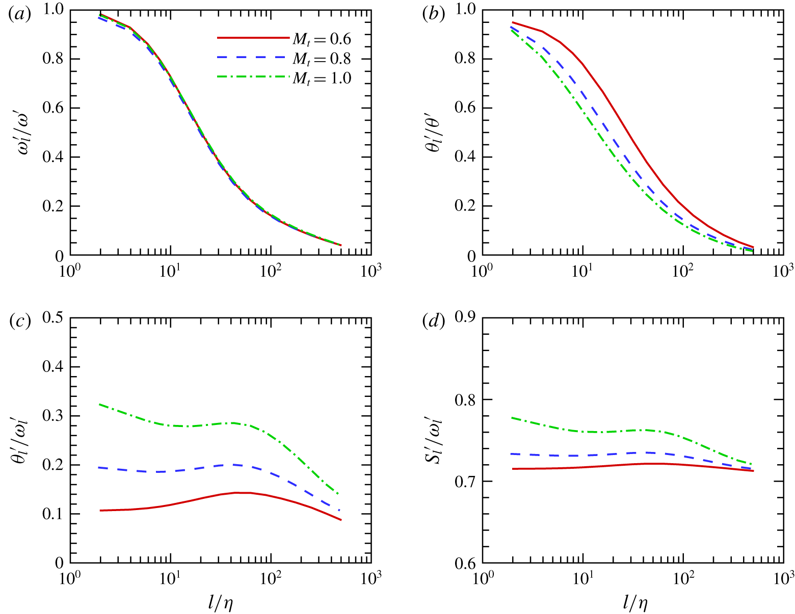
Normalized r.m.s. values of filtered vorticity, filtered velocity divergence and filtered strain-rate tensor: (a)  $\unicode[STIX]{x1D714}_{l}^{\prime }/\unicode[STIX]{x1D714}^{\prime }$; (b)
 $\unicode[STIX]{x1D703}_{l}^{\prime }/\unicode[STIX]{x1D703}^{\prime }$; (c)
 $\unicode[STIX]{x1D703}_{l}^{\prime }/\unicode[STIX]{x1D714}_{l}^{\prime }$; (d)
 $S_{l}^{\prime }/\unicode[STIX]{x1D714}_{l}^{\prime }$.

The SGS flux of kinetic energy  $\unicode[STIX]{x1D6F1}_{l}$ can be decomposed into a solenoidal component
 $\unicode[STIX]{x1D6F1}_{l}^{s}$ and a compressible component
 $\unicode[STIX]{x1D6F1}_{l}^{c}$:
 $\unicode[STIX]{x1D6F1}_{l}=\unicode[STIX]{x1D6F1}_{l}^{s}+\unicode[STIX]{x1D6F1}_{l}^{c}$ (Wang et al. Reference Wang, Wan, Chen and Chen2018a), where
 $$\begin{eqnarray}\unicode[STIX]{x1D6F1}_{l}^{s}\equiv -\overline{\unicode[STIX]{x1D70C}}\widetilde{\unicode[STIX]{x1D70F}}_{ij}\frac{\unicode[STIX]{x2202}}{\unicode[STIX]{x2202}x_{j}}\left(\frac{\widetilde{w}_{i}^{s}}{\sqrt{\overline{\unicode[STIX]{x1D70C}}}}\right)\end{eqnarray}$$
and
 $$\begin{eqnarray}\unicode[STIX]{x1D6F1}_{l}^{c}\equiv -\overline{\unicode[STIX]{x1D70C}}\widetilde{\unicode[STIX]{x1D70F}}_{ij}\frac{\unicode[STIX]{x2202}}{\unicode[STIX]{x2202}x_{j}}\left(\frac{\widetilde{w}_{i}^{c}}{\sqrt{\overline{\unicode[STIX]{x1D70C}}}}\right).\end{eqnarray}$$
The filtered vorticity and filtered velocity divergence are defined by  $\unicode[STIX]{x1D74E}_{l}=\unicode[STIX]{x1D735}\times \widetilde{\boldsymbol{u}}$ and
 $\unicode[STIX]{x1D703}_{l}=\unicode[STIX]{x1D735}\boldsymbol{\cdot }\widetilde{\boldsymbol{u}}$, respectively. The r.m.s. values of filtered vorticity, filtered velocity divergence and filtered strain-rate tensor are calculated by
 $\unicode[STIX]{x1D714}_{l}^{\prime }=\sqrt{\langle \unicode[STIX]{x1D74E}_{l}\boldsymbol{\cdot }\unicode[STIX]{x1D74E}_{l}\rangle }$,
 $\unicode[STIX]{x1D703}_{l}^{\prime }=\sqrt{\langle \unicode[STIX]{x1D703}_{l}^{2}\rangle }$ and
 $S_{l}^{\prime }=\sqrt{\langle \widetilde{\unicode[STIX]{x1D61A}}_{ij}\widetilde{\unicode[STIX]{x1D61A}}_{ij}\rangle }$, respectively. Figure 1 plots the normalized r.m.s. values of filtered vorticity, filtered velocity divergence and filtered strain-rate tensor at turbulent Mach numbers
 $M_{t}=0.6,0.8,1.0$. Both
 $\unicode[STIX]{x1D714}_{l}^{\prime }/\unicode[STIX]{x1D714}^{\prime }$ and
 $\unicode[STIX]{x1D703}_{l}^{\prime }/\unicode[STIX]{x1D703}^{\prime }$ decrease monotonically with the filter width
 $l$, which is close to
 $1$ at
 $l/\unicode[STIX]{x1D702}=4$ and close to
 $0$ at
 $l/\unicode[STIX]{x1D702}=512$. The effect of turbulent Mach number on
 $\unicode[STIX]{x1D714}_{l}^{\prime }/\unicode[STIX]{x1D714}^{\prime }$ is negligibly small. For a fixed filter width
 $l$,
 $\unicode[STIX]{x1D703}_{l}^{\prime }/\unicode[STIX]{x1D703}^{\prime }$ is slightly smaller at a larger turbulent Mach number. Thus, the effect of filter width on the r.m.s. values of vorticity and velocity divergence is similar, and is nearly independent of turbulent Mach number, implying that the coupling between the effects of length scale and compressibility is quite weak. At a given filter width
 $l$,
 $\unicode[STIX]{x1D714}_{l}^{\prime }$ and
 $\unicode[STIX]{x1D703}_{l}^{\prime }$ represent the overall strength of the solenoidal and compressible components of the filtered velocity gradient, respectively. The ratio
 $\unicode[STIX]{x1D703}_{l}^{\prime }/\unicode[STIX]{x1D714}_{l}^{\prime }$ gives the relative importance of the compressibility effect on the filtered velocity gradient;
 $\unicode[STIX]{x1D703}_{l}^{\prime }/\unicode[STIX]{x1D714}_{l}^{\prime }$ increases rapidly with an increase of the turbulent Mach number, similar to the behaviour of
 $\unicode[STIX]{x1D703}^{\prime }/\unicode[STIX]{x1D714}^{\prime }$. It is also found that
 $S_{l}^{\prime }/\unicode[STIX]{x1D714}_{l}^{\prime }$ becomes larger as the turbulent Mach number increases. Moreover, the dependence of both
 $\unicode[STIX]{x1D703}_{l}^{\prime }/\unicode[STIX]{x1D714}_{l}^{\prime }$ and
 $S_{l}^{\prime }/\unicode[STIX]{x1D714}_{l}^{\prime }$ on the filter width
 $l$ is relatively weak at
 $10\leqslant l/\unicode[STIX]{x1D702}\leqslant 100$, as compared to
 $\unicode[STIX]{x1D714}_{l}^{\prime }/\unicode[STIX]{x1D714}^{\prime }$ and
 $\unicode[STIX]{x1D703}_{l}^{\prime }/\unicode[STIX]{x1D703}^{\prime }$. It is well known that the flow statistics exhibit some scale-independent properties or power law scaling behaviours in the inertial range of incompressible turbulence. The study of scaling behaviours of
 $\unicode[STIX]{x1D703}_{l}^{\prime }/\unicode[STIX]{x1D714}_{l}^{\prime }$ and
 $S_{l}^{\prime }/\unicode[STIX]{x1D714}_{l}^{\prime }$ in the inertial range is critical to understanding the compressibility effect on the inertial dynamics of turbulence, and requires further numerical simulations at higher Reynolds numbers.
5 Local flow topology of filtered velocity gradient
The flow topology at small scales of a compressible flow field can be studied by the method of topological classification (Chong et al. Reference Chong, Perry and Cantwell1990) based on the three invariants of the velocity gradient tensor  $\unicode[STIX]{x1D608}_{ij}=\unicode[STIX]{x2202}u_{j}/\unicode[STIX]{x2202}x_{i}$. Similarly, the flow topology at a typical scale
 $l$ (
 $l>\unicode[STIX]{x1D702}$) of compressible turbulence can be investigated based on the three invariants of the filtered velocity gradient tensor
 $\widetilde{\unicode[STIX]{x1D608}}_{ij}=\unicode[STIX]{x2202}\widetilde{u}_{j}/\unicode[STIX]{x2202}x_{i}$, where
 $l$ is the filter width.
The three eigenvalues of the filtered velocity gradient tensor are denoted by  $\unicode[STIX]{x1D709}_{i}$ (
 $i=1,2,3$), which satisfy the following characteristic equation:
 $$\begin{eqnarray}\unicode[STIX]{x1D709}_{i}^{3}+P_{l}\unicode[STIX]{x1D709}_{i}^{2}+Q_{l}\unicode[STIX]{x1D709}_{i}+R_{l}=0.\end{eqnarray}$$
where  $P_{l}$,
 $Q_{l}$ and
 $R_{l}$ denote the first, second and third invariants of
 $\widetilde{\unicode[STIX]{x1D608}}_{ij}$, respectively, which are defined by
 $$\begin{eqnarray}\displaystyle & \displaystyle P_{l}=-(\unicode[STIX]{x1D709}_{1}+\unicode[STIX]{x1D709}_{2}+\unicode[STIX]{x1D709}_{3})=-\unicode[STIX]{x1D703}_{l}, & \displaystyle\end{eqnarray}$$
 $$\begin{eqnarray}\displaystyle & \displaystyle Q_{l}=\unicode[STIX]{x1D709}_{1}\unicode[STIX]{x1D709}_{2}+\unicode[STIX]{x1D709}_{2}\unicode[STIX]{x1D709}_{3}+\unicode[STIX]{x1D709}_{3}\unicode[STIX]{x1D709}_{1}={\textstyle \frac{1}{2}}(P_{l}^{2}-\widetilde{\unicode[STIX]{x1D61A}}_{ij}\widetilde{\unicode[STIX]{x1D61A}}_{ij}+\widetilde{\unicode[STIX]{x1D61E}}_{ij}\widetilde{\unicode[STIX]{x1D61E}}_{ij}), & \displaystyle\end{eqnarray}$$
 $$\begin{eqnarray}\displaystyle & \displaystyle R_{l}=-\unicode[STIX]{x1D709}_{1}\unicode[STIX]{x1D709}_{2}\unicode[STIX]{x1D709}_{3}={\textstyle \frac{1}{3}}(-P_{l}^{3}+3P_{l}Q_{l}-\widetilde{\unicode[STIX]{x1D61A}}_{ij}\widetilde{\unicode[STIX]{x1D61A}}_{jk}\widetilde{\unicode[STIX]{x1D61A}}_{ki}-3\widetilde{\unicode[STIX]{x1D61E}}_{ij}\widetilde{\unicode[STIX]{x1D61E}}_{jk}\widetilde{\unicode[STIX]{x1D61A}}_{ki}), & \displaystyle\end{eqnarray}$$
where  $\widetilde{\unicode[STIX]{x1D61A}}_{ij}=(\widetilde{\unicode[STIX]{x1D608}}_{ij}+\widetilde{\unicode[STIX]{x1D608}}_{ji})/2$ and
 $\widetilde{\unicode[STIX]{x1D61E}}_{ij}=(\widetilde{\unicode[STIX]{x1D608}}_{ij}-\widetilde{\unicode[STIX]{x1D608}}_{ji})/2$ are the filtered strain-rate tensor and filtered rotation-rate tensor, respectively.
The discriminant  $\unicode[STIX]{x1D6E5}_{l}$ of the filtered velocity gradient tensor is given by
 $$\begin{eqnarray}\unicode[STIX]{x1D6E5}_{l}=27R_{l}^{2}+(4P_{l}^{3}-18P_{l}Q_{l})R_{l}+(4Q_{l}^{3}-P_{l}^{2}Q_{l}^{2}).\end{eqnarray}$$
If  $\unicode[STIX]{x1D6E5}_{l}<0$, the three eigenvalues of
 $\widetilde{\unicode[STIX]{x1D608}}_{ij}$ are all real:
 $\unicode[STIX]{x1D709}_{1}\leqslant \unicode[STIX]{x1D709}_{2}\leqslant \unicode[STIX]{x1D709}_{3}$. On the other hand, if
 $\unicode[STIX]{x1D6E5}_{l}>0$, only one eigenvalue is real, and the two other eigenvalues are complex conjugate pairs:
 $\unicode[STIX]{x1D709}_{1,2}=\unicode[STIX]{x1D709}_{r}\pm \text{i}\unicode[STIX]{x1D709}_{i}$, and
 $\unicode[STIX]{x1D709}_{3}$ is real, where
 $\unicode[STIX]{x1D709}_{r}$ and
 $\unicode[STIX]{x1D709}_{i}$ are real numbers (Chong et al. Reference Chong, Perry and Cantwell1990);
 $\unicode[STIX]{x1D6E5}_{l}<0$ and
 $\unicode[STIX]{x1D6E5}_{l}>0$ correspond to the non-focal regions and focal regions of filtered velocity field, respectively. The surface
 $\unicode[STIX]{x1D6E5}_{l}=0$ can be split into two surfaces
 $r^{(1a)}$ and
 $r^{(1b)}$, given by
 $$\begin{eqnarray}\displaystyle & \displaystyle P_{l}(9Q_{l}-2P_{l}^{2})-2(-3Q_{l}+P_{l}^{2})^{3/2}-27R_{l}=0, & \displaystyle\end{eqnarray}$$
 $$\begin{eqnarray}\displaystyle & \displaystyle P_{l}(9Q_{l}-2P_{l}^{2})+2(-3Q_{l}+P_{l}^{2})^{3/2}-27R_{l}=0. & \displaystyle\end{eqnarray}$$
The two surfaces  $r^{(1a)}$ and
 $r^{(1b)}$ osculate each other to form a cusp. In the region
 $\unicode[STIX]{x1D6E5}_{l}>0$, there is another surface
 $r^{(2)}$ which contains the points associated with purely imaginary eigenvalues
 $$\begin{eqnarray}P_{l}Q_{l}-R_{l}=0.\end{eqnarray}$$
The surfaces  $r^{(1a)}$,
 $r^{(1b)}$,
 $r^{(2)}$ and
 $R_{l}=0$ divide the
 $P_{l}\,{-}\,Q_{l}\,{-}\,R_{l}$ space into different spatial regions (Chong et al. Reference Chong, Perry and Cantwell1990).
The flow topology of the filtered velocity field can be investigated conveniently on the  $Q_{l}\,{-}\,R_{l}$ plane for a given value of
 $P_{l}$ or
 $\unicode[STIX]{x1D703}_{l}$ (Suman & Girimaji Reference Suman and Girimaji2010; Wang & Lu Reference Wang and Lu2012). The surfaces
 $r^{(1a)}$,
 $r^{(1b)}$,
 $r^{(2)}$ and
 $R_{l}=0$ appear as curves on the
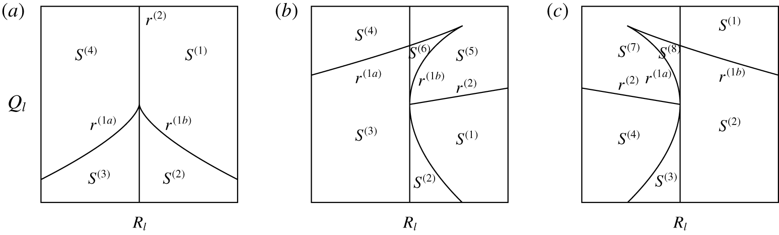
 $Q_{l}\,{-}\,R_{l}$ plane, dividing the plane into different regions corresponding to different topologies. The topological classifications of three representative
 $Q_{l}\,{-}\,R_{l}$ planes are shown in figure 2:
 $P_{l}=0$,
 $P_{l}>0$ and
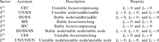
 $P_{l}<0$. A description of the cases for various flow topologies is listed in table 2 (Suman & Girimaji Reference Suman and Girimaji2010; Wang & Lu Reference Wang and Lu2012).
On the  $Q_{l}\,{-}\,R_{l}$ plane with
 $P_{l}=0$, the curves
 $r^{(1a)}$ and
 $r^{(1b)}$ are symmetric to each other with respect to the
 $Q_{l}$-axis, and the curve
 $r^{(2)}$ is coincident with the
 $Q_{l}$-axis. Four different topologies can be identified: UFC, UN/S/S, SN/S/S and SFS, which are denoted by
 $S^{(1)}$,
 $S^{(2)}$,
 $S^{(3)}$ and
 $S^{(4)}$, respectively. The UN/S/S and SN/S/S are non-focal structures associated with
 $\unicode[STIX]{x1D6E5}_{l}<0$, while UFC and SFS are focal structures associated with
 $\unicode[STIX]{x1D6E5}_{l}>0$.
On the  $Q_{l}\,{-}\,R_{l}$ plane with
 $P_{l}>0$, the curves
 $r^{(1a)}$ and
 $r^{(1b)}$ are no longer symmetric to each other, and the curve
 $r^{(2)}$ intersects with the curve
 $r^{(1b)}$ at
 $Q_{l}=0$ and
 $R_{l}=0$. Six different topologies can be identified: UFC, UN/S/S, SN/S/S, SFS, SFC and SN/SN/SN, which are denoted by
 $S^{(1)}$,
 $S^{(2)}$,
 $S^{(3)}$,
 $S^{(4)}$,
 $S^{(5)}$ and
 $S^{(6)}$, respectively.
On the  $Q_{l}\,{-}\,R_{l}$ plane with
 $P_{l}<0$, the curve
 $r^{(2)}$ intersects with the curve
 $r^{(1a)}$ at
 $Q_{l}=0$ and
 $R_{l}=0$. Six different topologies can be identified: UFC, UN/S/S, SN/S/S, SFS, UFS and UN/UN/UN, which are denoted by
 $S^{(1)}$,
 $S^{(2)}$,
 $S^{(3)}$,
 $S^{(4)}$,
 $S^{(7)}$ and
 $S^{(8)}$, respectively.
The topological classifications of three representative  $Q_{l}\,{-}\,R_{l}$ planes: (a)
 $P_{l}=0$, (b)
 $P_{l}>0$ and (c)
 $P_{l}<0$. A description of the cases for various flow topologies is provided in table 2.

Description of cases of various flow topological types.

6 Effect of flow topology on the kinetic energy flux
6.1 Statistical properties of the invariants of the filtered velocity gradient tensor
We investigate the joint PDF of the second and third invariants  $\text{PDF}(Q_{l},R_{l})$ of the filtered velocity gradient tensor for three filter widths
 $l/\unicode[STIX]{x1D702}=4,16,64$, for three ranges of filtered velocity divergence: (i)
 $-0.05\leqslant \unicode[STIX]{x1D703}_{l}/\unicode[STIX]{x1D703}_{l}^{\prime }\leqslant 0.05$; (ii)
 $-3.15\leqslant \unicode[STIX]{x1D703}_{l}/\unicode[STIX]{x1D703}_{l}^{\prime }\leqslant -2.85$; and (iii)
 $2.85\leqslant \unicode[STIX]{x1D703}_{l}/\unicode[STIX]{x1D703}_{l}^{\prime }\leqslant 3.15$, approximately corresponding to three values of the normalized first invariant: (i)
 $P_{l}/P_{l}^{\prime }\approx 0$; (ii)
 $P_{l}/P_{l}^{\prime }\approx 3$; and (iii)
 $P_{l}/P_{l}^{\prime }\approx -3$, respectively. Here,
 $P_{l}^{\prime }=\sqrt{\langle P_{l}^{2}\rangle }=\unicode[STIX]{x1D703}_{l}^{\prime }$. The second and third invariants of the filtered velocity gradient tensor can be normalized as
 $Q_{l}/\langle Q_{l,W}\rangle$ and
 $R_{l}/\langle Q_{l,W}\rangle ^{3/2}$, respectively, where
 $Q_{l,W}$ is the second invariant of the filtered rotation-rate tensor, defined by
 $Q_{l,W}=\widetilde{\unicode[STIX]{x1D61E}}_{ij}\widetilde{\unicode[STIX]{x1D61E}}_{ij}/2=(1/4)(\widetilde{\unicode[STIX]{x1D714}}_{l})^{2}$.
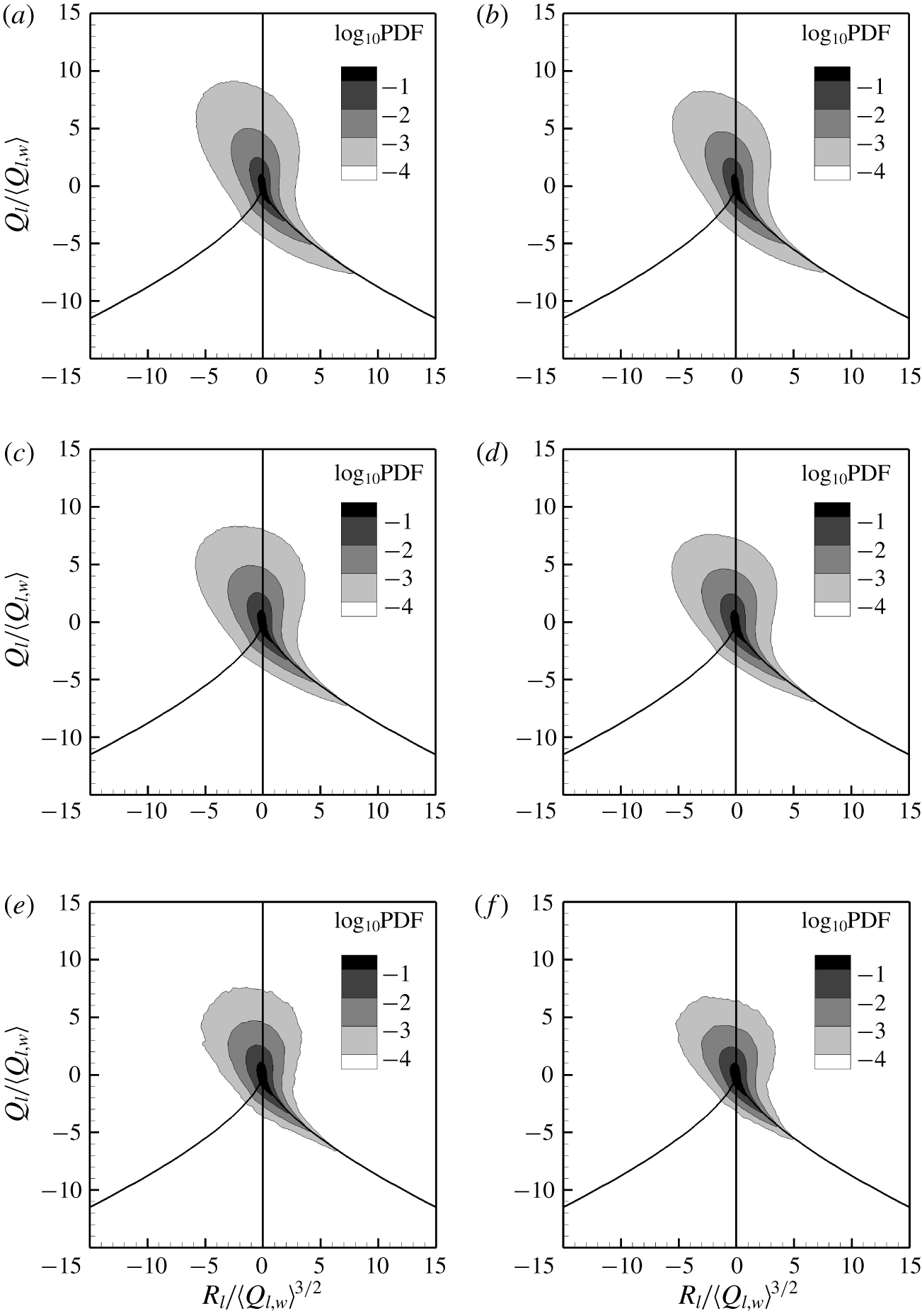
Logarithm of joint PDF of the second and third invariants of the filtered velocity gradient tensor  $\log _{10}\text{PDF}(Q_{l},R_{l})$, at
 $M_{t}=0.6,1.0$, for three filter widths
 $l/\unicode[STIX]{x1D702}=4,16,64$, in the range of filtered velocity divergence
 $-0.05\leqslant \unicode[STIX]{x1D703}_{l}/\unicode[STIX]{x1D703}_{l}^{\prime }\leqslant 0.05$: (a,b)
 $l/\unicode[STIX]{x1D702}=4$, (c,d)
 $l/\unicode[STIX]{x1D702}=16$ and (e,f)
 $l/\unicode[STIX]{x1D702}=64$. (a,c,e)
 $M_{t}=0.6$; (b,d,f)
 $M_{t}=1.0$. The second and third invariants are normalized as
 $Q_{l}/\langle Q_{l,W}\rangle$ and
 $R_{l}/\langle Q_{l,W}\rangle ^{3/2}$, respectively.

Figure 3 plots the iso-contour lines of the joint PDF of the second and third invariants of the filtered velocity gradient tensor at  $M_{t}=0.6,1.0$, for three filter widths
 $l/\unicode[STIX]{x1D702}=4,16,64$, in the range of filtered velocity divergence
 $-0.05\leqslant \unicode[STIX]{x1D703}_{l}/\unicode[STIX]{x1D703}_{l}^{\prime }\leqslant 0.05$. It is shown that the iso-contour lines of the joint PDF for the nearly incompressible region
 $-0.05\leqslant \unicode[STIX]{x1D703}_{l}/\unicode[STIX]{x1D703}_{l}^{\prime }\leqslant 0.05$ (
 $P_{l}/P_{l}^{\prime }\approx 0$) at
 $l/\unicode[STIX]{x1D702}=4$ exhibit teardrop shapes, which are similar to those of the velocity gradient tensor in compressible isotropic turbulence (Suman & Girimaji Reference Suman and Girimaji2010) and a compressible turbulent boundary layer (Wang & Lu Reference Wang and Lu2012). The iso-contour lines of the joint PDF at
 $l/\unicode[STIX]{x1D702}=16,64$ are qualitatively similar to those at
 $l/\unicode[STIX]{x1D702}=4$, in the nearly incompressible region
 $-0.05\leqslant \unicode[STIX]{x1D703}_{l}/\unicode[STIX]{x1D703}_{l}^{\prime }\leqslant 0.05$. It is observed that as
 $l/\unicode[STIX]{x1D702}$ is increased from
 $4$ to
 $64$, the shape of the joint PDF becomes broader and shorter, suggesting that the fractions of the
 $S^{(1)}$ and
 $S^{(4)}$ topological types increase and that of
 $S^{(2)}$ decreases. These observations are consistent with a previous analysis on the joint PDF of the invariants of the filtered velocity gradient tensor in incompressible isotropic turbulence (Danish & Meneveau Reference Danish and Meneveau2018). Therefore, in the nearly incompressible region
 $-0.05\leqslant \unicode[STIX]{x1D703}_{l}/\unicode[STIX]{x1D703}_{l}^{\prime }\leqslant 0.05$, we conclude that the effect of the turbulent Mach number on the joint PDF of the second and third invariants of the filtered velocity gradient tensor is weak.
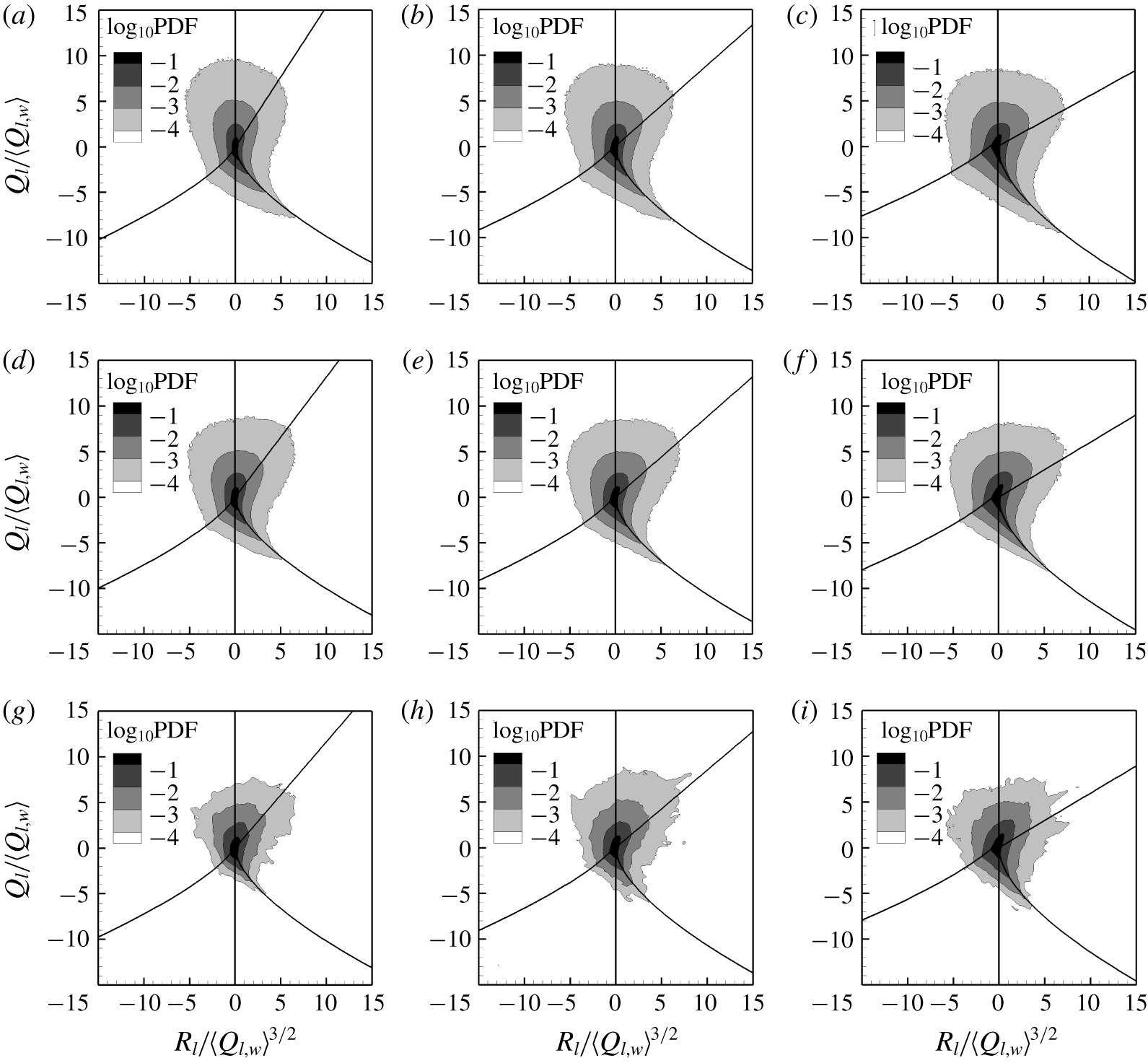
Logarithm of the joint PDF of the second and third invariants of the filtered velocity gradient tensor  $\log _{10}\text{PDF}(Q_{l},R_{l})$, at
 $M_{t}=0.6,0.8,1.0$, for three filter widths
 $l/\unicode[STIX]{x1D702}=4,16,64$, in the range of filtered velocity divergence
 $-3.15\leqslant \unicode[STIX]{x1D703}_{l}/\unicode[STIX]{x1D703}_{l}^{\prime }\leqslant -2.85$: (a–c)
 $l/\unicode[STIX]{x1D702}=4$, (d–f)
 $l/\unicode[STIX]{x1D702}=16$ and (g–i)
 $l/\unicode[STIX]{x1D702}=64$. (a,d,g)
 $M_{t}=0.6$; (b,e,h)
 $M_{t}=0.8$; (c,f,i)
 $M_{t}=1.0$. The second and third invariants are normalized as
 $Q_{l}/\langle Q_{l,W}\rangle$ and
 $R_{l}/\langle Q_{l,W}\rangle ^{3/2}$, respectively.

Figure 4 depicts the iso-contour lines of the same joint PDF at  $M_{t}=0.6,0.8,1.0$, for three filter widths
 $l/\unicode[STIX]{x1D702}=4,16,64$, in the compression range
 $-3.15\leqslant \unicode[STIX]{x1D703}_{l}/\unicode[STIX]{x1D703}_{l}^{\prime }\leqslant -2.85$. The irregular fluctuation of iso-contour lines of the joint PDF at
 $l/\unicode[STIX]{x1D702}=64$ is due to the lack of samples. As compared to the situation of the nearly incompressible region
 $-0.05\leqslant \unicode[STIX]{x1D703}_{l}/\unicode[STIX]{x1D703}_{l}^{\prime }\leqslant 0.05$, the iso-contour lines of the joint PDF of the second and third invariants in the compression region (
 $P_{l}/P_{l}^{\prime }\approx 3$) become wider, and the fractions of the iso-contour lines occupying the first and third quadrants become larger. This observation implies that the
 $S^{(3)}$ and
 $S^{(5)}$ topological types take a larger fraction in the compression region than those in the nearly incompressible region. It is also shown that these
 $S^{(3)}$ and
 $S^{(5)}$ fractions can be enhanced by an increase of the turbulent Mach number in the compression region.
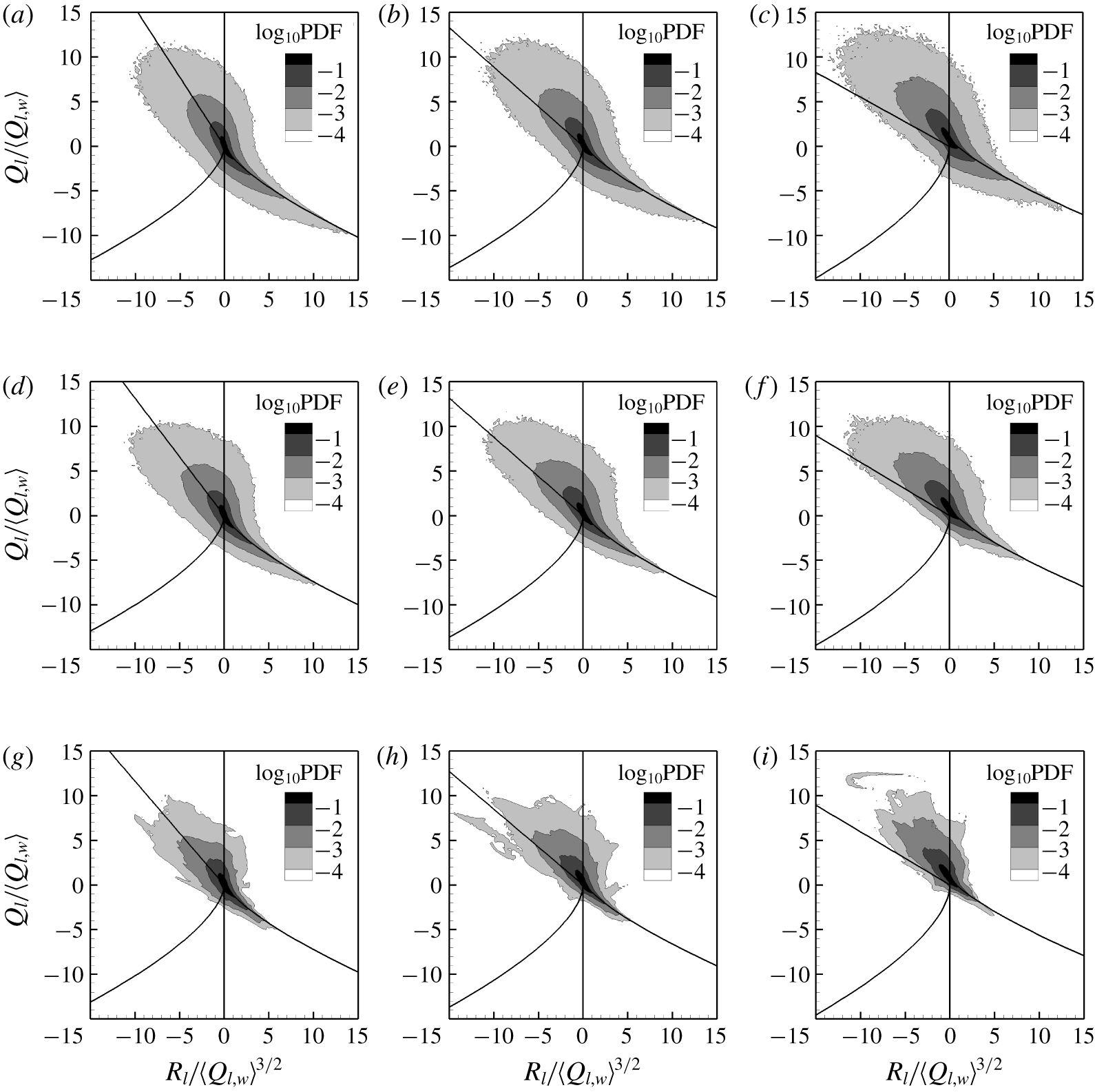
Logarithm of joint PDF of the second and third invariants of the filtered velocity gradient tensor  $\log _{10}\text{PDF}(Q_{l},R_{l})$, at
 $M_{t}=0.6,0.8,1.0$, for three filter widths
 $l/\unicode[STIX]{x1D702}=4,16,64$, in the range of filtered velocity divergence
 $2.85\leqslant \unicode[STIX]{x1D703}_{l}/\unicode[STIX]{x1D703}_{l}^{\prime }\leqslant 3.15$: (a–c)
 $l/\unicode[STIX]{x1D702}=4$, (d–f)
 $l/\unicode[STIX]{x1D702}=16$ and (g–i)
 $l/\unicode[STIX]{x1D702}=64$. (a,d,g)
 $M_{t}=0.6$; (b,e,h)
 $M_{t}=0.8$; (c,f,i)
 $M_{t}=1.0$. The second and third invariants are normalized as
 $Q_{l}/\langle Q_{l,W}\rangle$ and
 $R_{l}/\langle Q_{l,W}\rangle ^{3/2}$, respectively.

Figure 5 shows the iso-contour lines of the same joint PDF at  $M_{t}=0.6,0.8,1.0$, for three filter widths
 $l/\unicode[STIX]{x1D702}=4,16,64$, in the expansion range
 $2.85\leqslant \unicode[STIX]{x1D703}_{l}/\unicode[STIX]{x1D703}_{l}^{\prime }\leqslant 3.15$. Again the irregular fluctuation of the iso-contour lines of the joint PDF at
 $l/\unicode[STIX]{x1D702}=64$ is due to the lack of samples. The iso-contour lines of the joint PDF in the expansion region (
 $P_{l}/P_{l}^{\prime }\approx -3$) at
 $l/\unicode[STIX]{x1D702}=4$ have a tendency to occupy the second and fourth quadrants, and exhibit more skewed shapes as compared to those of the nearly incompressible region
 $-0.05\leqslant \unicode[STIX]{x1D703}_{l}/\unicode[STIX]{x1D703}_{l}^{\prime }\leqslant 0.05$. This observation indicates that, for the filter width
 $l/\unicode[STIX]{x1D702}=4$, the fractions of
 $S^{(2)}$ and
 $S^{(7)}$ topological types are larger in the expansion region than those in the nearly incompressible region. In addition, the fraction of
 $S^{(7)}$ topology at
 $l/\unicode[STIX]{x1D702}=4$ in the expansion region can be enhanced by an increase of the turbulent Mach number. It is revealed that, as the filter width
 $l$ increases, the fractions of the joint PDF in the third and fourth quadrants become smaller in the expansion region.
6.2 Statistical relation between the invariants of the filtered velocity gradient tensor and SGS kinetic energy flux
In order to examine the statistical relation between the invariants of filtered velocity gradient tensor and SGS kinetic energy flux, we consider the relative contribution of each region in the  $Q_{l}\,{-}\,R_{l}$ plane to the SGS kinetic energy flux for a given range of filtered velocity divergence
 $\unicode[STIX]{x1D703}_{l,1}\leqslant \unicode[STIX]{x1D703}_{l}\leqslant \unicode[STIX]{x1D703}_{l,2}$, which is defined by (Wang et al. Reference Wang, Shi, Wang, Xiao, He and Chen2012)
 $$\begin{eqnarray}F_{KEF}(Q_{l},R_{l})=\frac{f_{KEF}(Q_{l},R_{l})\text{PDF}(Q_{l},R_{l})}{\displaystyle \int _{-\infty }^{\infty }\int _{-\infty }^{\infty }f_{KEF}(Q_{l},R_{l})\text{PDF}(Q_{l},R_{l})\,\text{d}Q_{l}\,\text{d}R_{l}},\end{eqnarray}$$
where  $\text{PDF}(Q_{l},R_{l})$ is the joint PDF of
 $(Q_{l},R_{l})$ for
 $\unicode[STIX]{x1D703}_{l,1}\leqslant \unicode[STIX]{x1D703}_{l}\leqslant \unicode[STIX]{x1D703}_{l,2}$;
 $f_{KEF}(Q_{l},R_{l})$ is the average of SGS kinetic energy flux
 $\unicode[STIX]{x1D6F1}_{l}$ conditioned on
 $(Q_{l},R_{l})$ for
 $\unicode[STIX]{x1D703}_{l,1}\leqslant \unicode[STIX]{x1D703}_{l}\leqslant \unicode[STIX]{x1D703}_{l,2}$. The function
 $F_{KEF}(Q_{l},R_{l})$ has the following property:
 $$\begin{eqnarray}\int _{-\infty }^{\infty }\int _{-\infty }^{\infty }F_{KEF}(Q,R)\,\text{d}Q\,\text{d}R=1.\end{eqnarray}$$
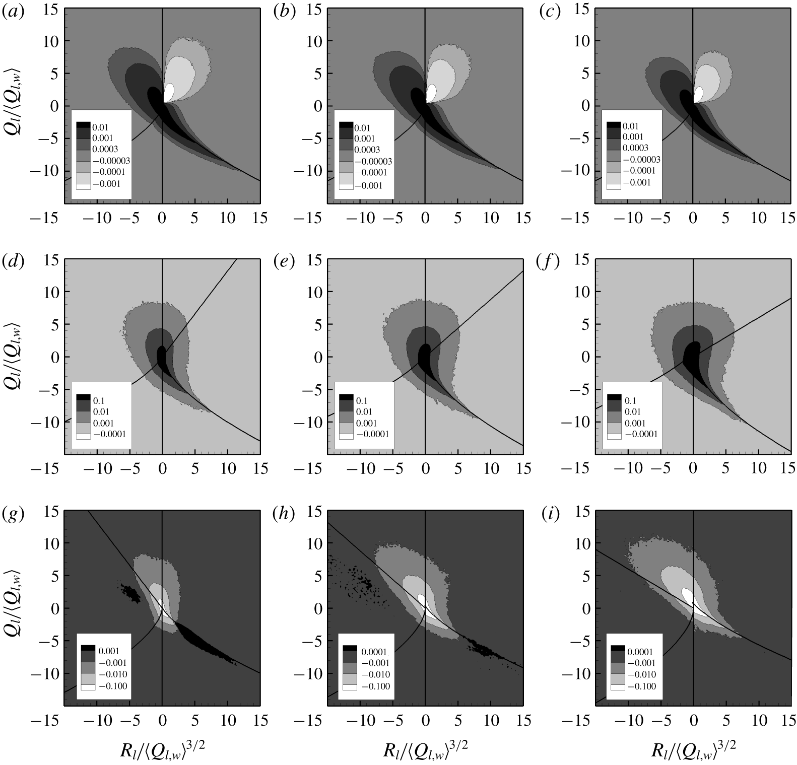
Figure 6 plots the relative contribution of each region of the  $Q_{l}\,{-}\,R_{l}$ plane to the SGS kinetic energy flux
 $F_{KEF}(Q_{l},R_{l})$, at
 $M_{t}=0.6,0.8,1.0$, for the filter width
 $l/\unicode[STIX]{x1D702}=16$, in three ranges of filtered velocity divergence:
 $-0.05\leqslant \unicode[STIX]{x1D703}_{l}/\unicode[STIX]{x1D703}_{l}^{\prime }\leqslant 0.05$,
 $-3.15\leqslant \unicode[STIX]{x1D703}_{l}/\unicode[STIX]{x1D703}_{l}^{\prime }\leqslant -2.85$ and
 $2.85\leqslant \unicode[STIX]{x1D703}_{l}/\unicode[STIX]{x1D703}_{l}^{\prime }\leqslant 3.15$. The contour lines of
 $F_{KEF}(Q_{l},R_{l})$ in the nearly incompressible region
 $-0.05\leqslant \unicode[STIX]{x1D703}_{l}/\unicode[STIX]{x1D703}_{l}^{\prime }\leqslant 0.05$ exhibit a butterfly-like shape. The contour lines of positive
 $F_{KEF}(Q_{l},R_{l})$ are found to exhibit teardrop shapes with a statistical preference for the second and fourth quadrants, similar to those of
 $\text{PDF}(Q_{l},R_{l})$. The positive part of
 $F_{KEF}(Q_{l},R_{l})$ predominates over its negative counterpart, indicating that kinetic energy has a tendency to be transferred from large scales to small scales by the SGS flux
 $\unicode[STIX]{x1D6F1}_{l}$. Moreover, the
 $S^{(2)}$ and
 $S^{(4)}$ topological types, corresponding to the second and fourth quadrants, make major contributions to the positive SGS kinetic energy flux
 $\unicode[STIX]{x1D6F1}_{l}$ in the nearly incompressible region. The effect of turbulent Mach number on
 $F_{KEF}(Q_{l},R_{l})$ is shown to be weak in the nearly incompressible region (
 $-0.05\leqslant \unicode[STIX]{x1D703}_{l}/\unicode[STIX]{x1D703}_{l}^{\prime }\leqslant 0.05$).
The relative contribution of each region of the  $Q_{l}\,{-}\,R_{l}$ plane to the SGS kinetic energy flux
 $F_{KEF}(Q_{l},R_{l})$, at
 $M_{t}=0.6,0.8,1.0$, for the filter width
 $l/\unicode[STIX]{x1D702}=16$, in three ranges of filtered velocity divergence: (a–c)
 $-0.05\leqslant \unicode[STIX]{x1D703}_{l}/\unicode[STIX]{x1D703}_{l}^{\prime }\leqslant 0.05$, (d–f)
 $-3.15\leqslant \unicode[STIX]{x1D703}_{l}/\unicode[STIX]{x1D703}_{l}^{\prime }\leqslant -2.85$ and (g–i)
 $2.85\leqslant \unicode[STIX]{x1D703}_{l}/\unicode[STIX]{x1D703}_{l}^{\prime }\leqslant 3.15$. (a,d,g)
 $M_{t}=0.6$; (b,e,h)
 $M_{t}=0.8$; (c,f,i)
 $M_{t}=1.0$. The second and third invariants of the velocity gradient tensor are normalized as
 $Q_{l}/\langle Q_{l,W}\rangle$ and
 $R_{l}/\langle Q_{l,W}\rangle ^{3/2}$, respectively.

In the compression region ( $-3.15\leqslant \unicode[STIX]{x1D703}_{l}/\unicode[STIX]{x1D703}_{l}^{\prime }\leqslant -2.85$), only contour lines of positive
 $F_{KEF}(Q,R)$ can be observed, and exhibit wider shapes as compared to the situation of the nearly incompressible region. This observation implies that the direct SGS flux of kinetic energy from large scales to small scales can be enhanced by compression motions. The contour lines of positive
 $F_{KEF}(Q,R)$ are quite similar to those of
 $\text{PDF}(Q_{l},R_{l})$. As the turbulent Mach number increases, the contour lines of positive
 $F_{KEF}(Q,R)$ become wider, due to the stronger effect of compressibility.
It is found that the contour lines of negative  $F_{KEF}(Q,R)$ are predominant over those of positive
 $F_{KEF}(Q,R)$ in the expansion region (
 $2.85\leqslant \unicode[STIX]{x1D703}_{l}/\unicode[STIX]{x1D703}_{l}^{\prime }\leqslant 3.15$). Thus, expansion motions can enhance the reverse SGS flux of kinetic energy from small scales to large scales, which are opposite to compression motions. The contour lines of negative
 $F_{KEF}(Q,R)$ become wider with the increase of turbulent Mach number in the expansion region, suggesting that the reverse SGS flux of kinetic energy becomes more significant at higher turbulent Mach numbers.
6.3 Statistical properties of kinetic energy flux in various flow topologies
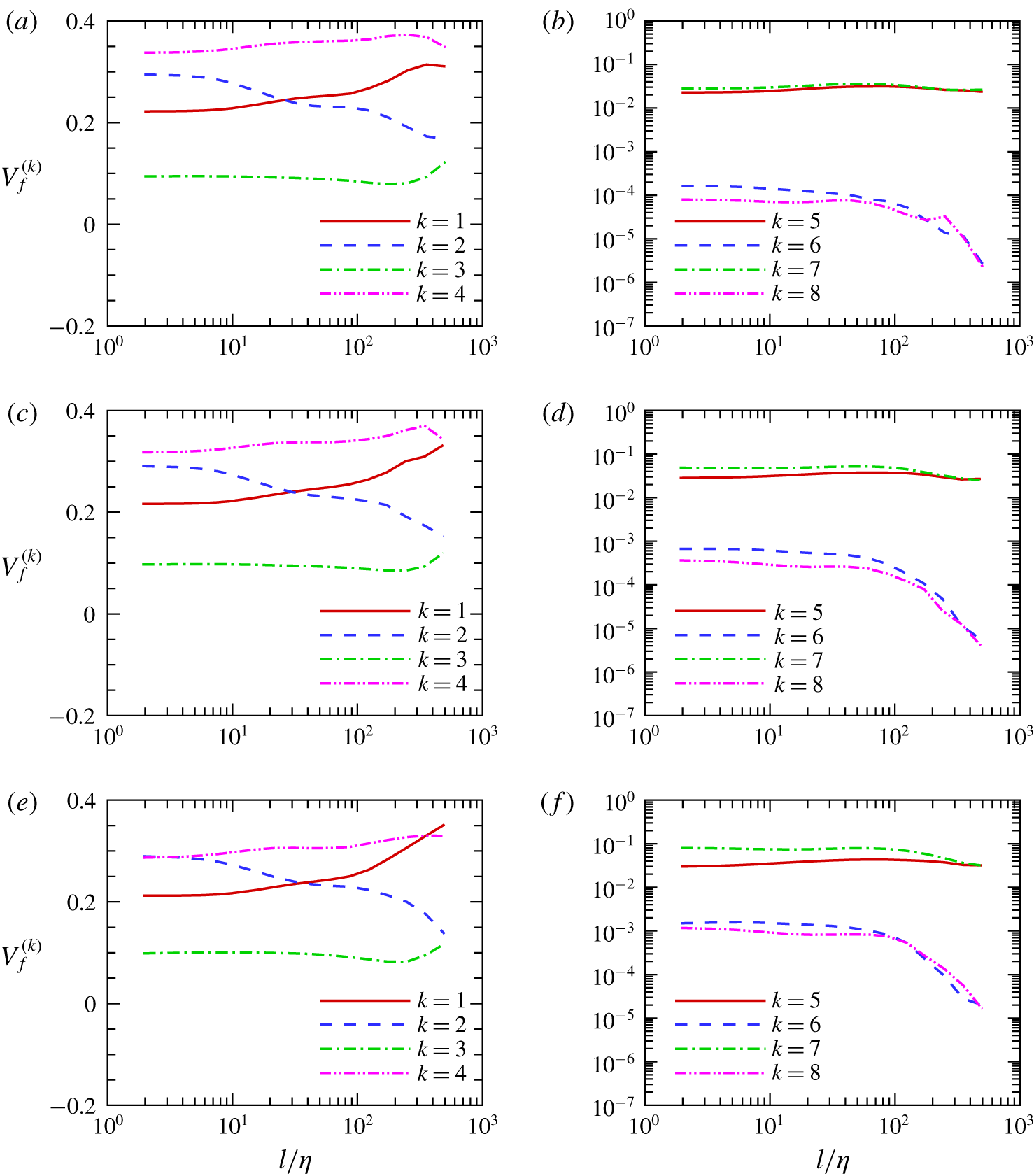
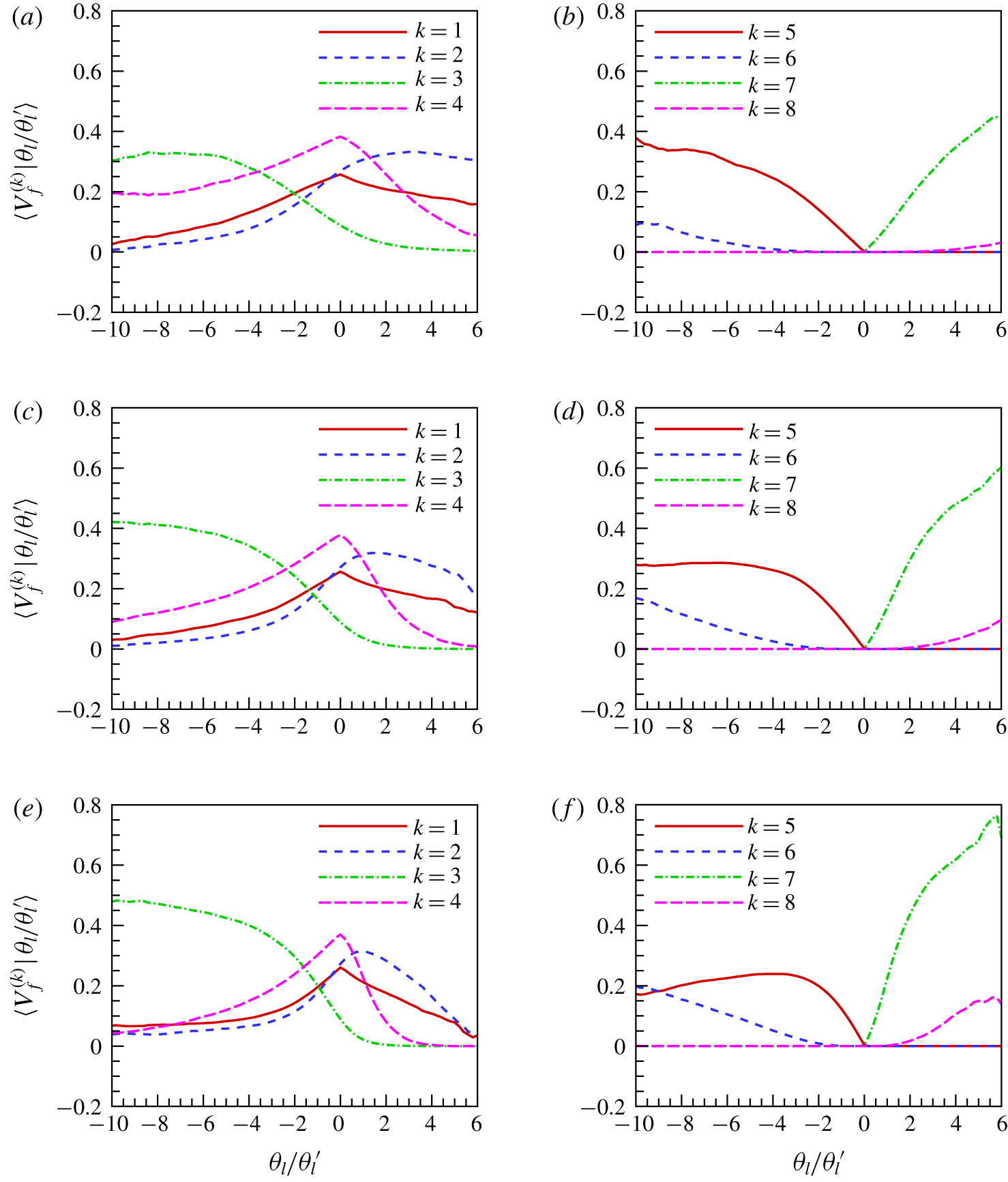
The multiscale statistical properties of the velocity field can be characterized conveniently by the volume fractions  $V_{f}^{(k)}$ of various flow topological types
 $S^{(k)}$ of the filtered velocity gradient tensor in compressible isotropic turbulence. Figure 7 shows the volume fractions
 $V_{f}^{(k)}$ of various flow topologies
 $S^{(k)}$ at turbulent Mach numbers
 $M_{t}=0.6,0.8,1.0$. The volume fractions of
 $S^{(1)}$,
 $S^{(2)}$ and
 $S^{(4)}$ topological types are always larger than those of the other five, similar to the results for incompressible isotropic turbulence (Danish & Meneveau Reference Danish and Meneveau2018), decaying compressible isotropic turbulence (Suman & Girimaji Reference Suman and Girimaji2010) and a compressible turbulent boundary layer (Wang & Lu Reference Wang and Lu2012).
Volume fractions  $V_{f}^{(k)}$ of various flow topologies
 $S^{(k)}$. (a,b)
 $M_{t}=0.6$; (c,d)
 $M_{t}=0.8$; (e,f)
 $M_{t}=1.0$.

At the small scale  $l/\unicode[STIX]{x1D702}=2$, more than half of flow field can be characterized by the
 $S^{(2)}$ or
 $S^{(4)}$ topological types, and the volume fraction of the
 $S^{(1)}$ topology is smaller than those of
 $S^{(2)}$ and
 $S^{(4)}$. As the filter width becomes larger, the volume fractions of
 $S^{(1)}$ and
 $S^{(4)}$ topological types increase slightly, while the
 $S^{(2)}$ volume fraction decreases. At large scale
 $l/\unicode[STIX]{x1D702}=512$, the
 $S^{(2)}$ volume fraction is significantly smaller than those of
 $S^{(1)}$ and
 $S^{(4)}$. It is found that the volume fraction of the
 $S^{(4)}$ topology decreases with the increase of the turbulent Mach number. The volume fraction of the
 $S^{(4)}$ topology is always the largest at all scales for
 $M_{t}=0.6$, but is no longer the largest at small scale
 $l/\unicode[STIX]{x1D702}=2$ and large scale
 $l/\unicode[STIX]{x1D702}=512$ for
 $M_{t}=1.0$. The volume fraction of the
 $S^{(3)}$ topology is close to
 $10\,\%$ at scales
 $l/\unicode[STIX]{x1D702}\leqslant 200$, and slightly increases as the filter width
 $l/\unicode[STIX]{x1D702}$ is increased further above
 $200$. The effect of turbulent Mach number on the volume fraction of the
 $S^{(3)}$ topology is negligibly small. These observations are similar to the results on the population fractions of various topologies for the filtered velocity field in incompressible isotropic turbulence (Danish & Meneveau Reference Danish and Meneveau2018).
The topologies  $S^{(5)}$,
 $S^{(6)}$,
 $S^{(7)}$ and
 $S^{(8)}$ can be identified only for compressible flows. Due to the effect of compressibility, the volume fractions of
 $S^{(5)}$,
 $S^{(6)}$,
 $S^{(7)}$ and
 $S^{(8)}$ topological types increase significantly with the increase of the turbulent Mach number. It is found that the total volume fraction of
 $S^{(5)}$,
 $S^{(6)}$,
 $S^{(7)}$ and
 $S^{(8)}$ types is smaller than
 $15\,\%$ at turbulent Mach numbers
 $M_{t}=0.6,0.8,1.0$. The effect of filter width on the volume fractions of
 $S^{(5)}$,
 $S^{(6)}$,
 $S^{(7)}$ and
 $S^{(8)}$ is very weak when
 $l/\unicode[STIX]{x1D702}\leqslant 100$. As the filter width
 $l/\unicode[STIX]{x1D702}$ increases further above
 $100$, the volume fractions of
 $S^{(5)}$ and
 $S^{(7)}$ decrease slightly, while the volume fractions of
 $S^{(6)}$ and
 $S^{(8)}$ decrease rapidly. The volume fractions of
 $S^{(6)}$ and
 $S^{(8)}$ are always much smaller than those of
 $S^{(5)}$ and
 $S^{(7)}$ at the three turbulent Mach numbers considered here.
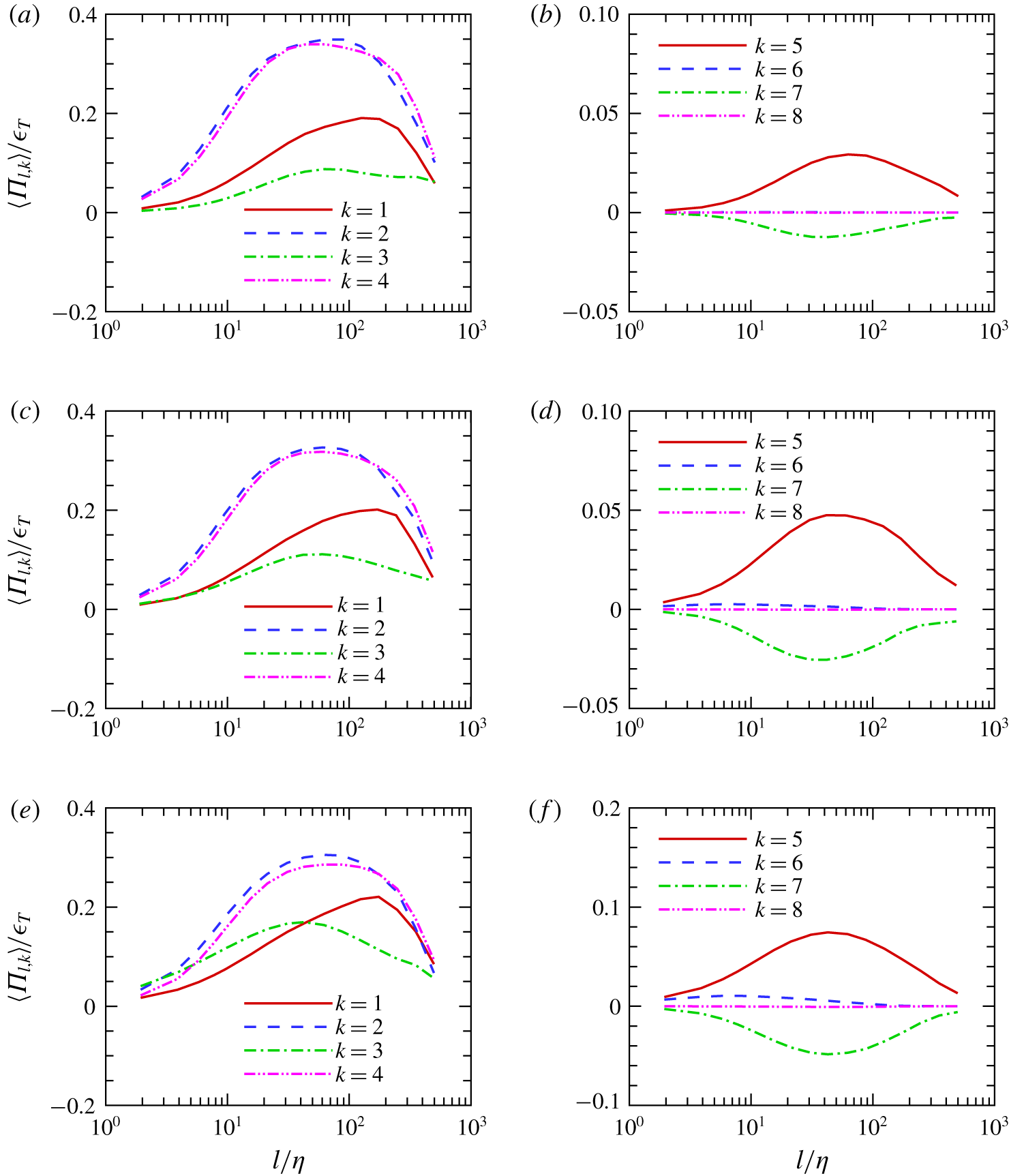
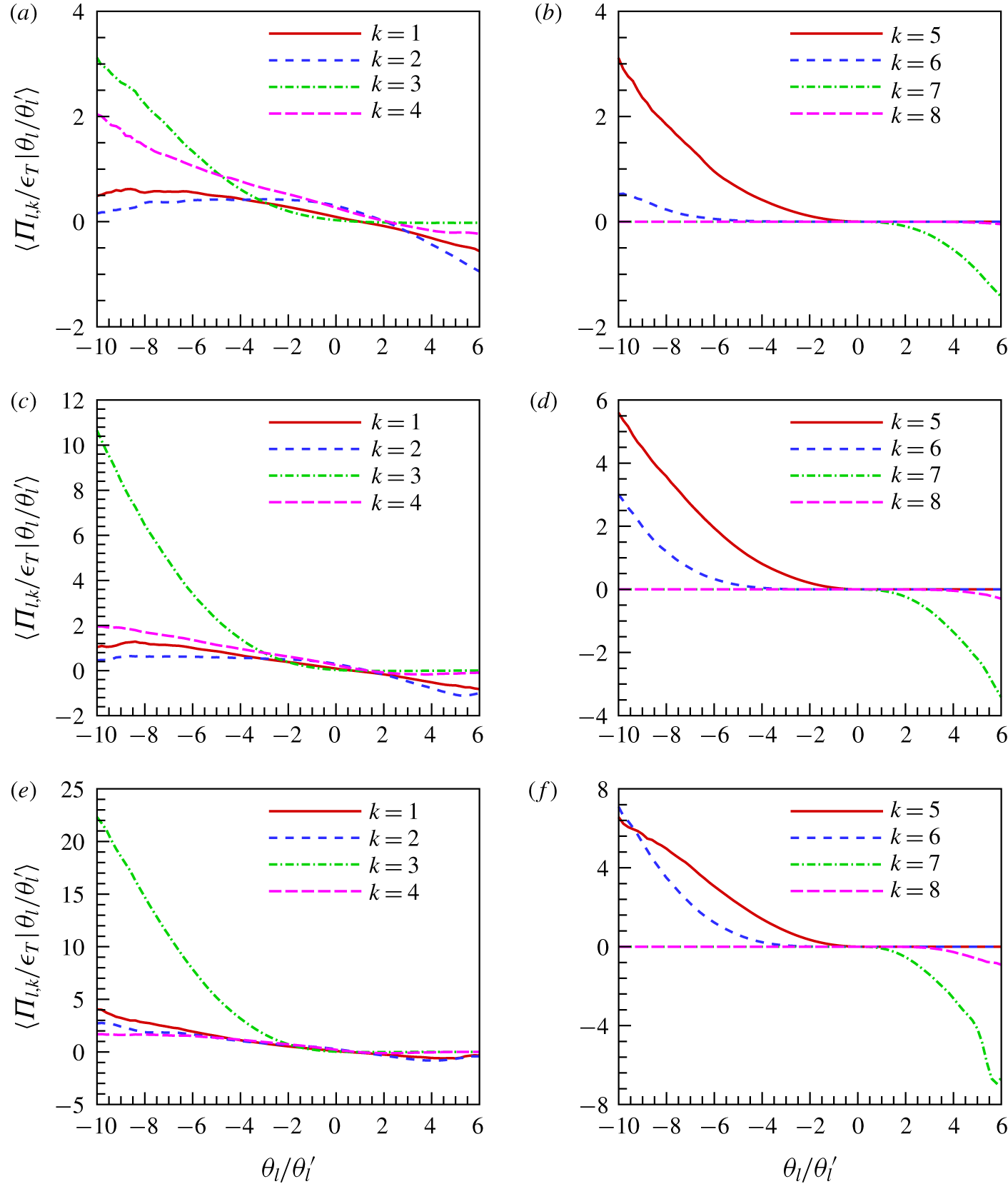
The average of contributions  $\langle \unicode[STIX]{x1D6F1}_{l,k}\rangle /\unicode[STIX]{x1D716}_{T}$ of various flow topologies
 $S^{(k)}$ to the normalized SGS kinetic energy flux
 $\unicode[STIX]{x1D6F1}_{l}/\unicode[STIX]{x1D716}_{T}$. (a,b)
 $M_{t}=0.6$; (c,d)
 $M_{t}=0.8$; (e,f)
 $M_{t}=1.0$.

In order to investigate the effect of flow topology on the SGS kinetic energy flux, we define the contribution  $\unicode[STIX]{x1D6F1}_{l,k}$ from the type-
 $k$ (
 $S^{(k)}$) topology to the SGS kinetic energy flux
 $\unicode[STIX]{x1D6F1}_{l}$ as follows:
 $\unicode[STIX]{x1D6F1}_{l,k}=\unicode[STIX]{x1D6F1}_{l}$ if the point is located in the
 $S^{(k)}$ topological region; otherwise, we set
 $\unicode[STIX]{x1D6F1}_{l,k}=0$. Similarly, the contribution
 $\unicode[STIX]{x1D6F1}_{l,k}^{s}$ to the solenoidal component of the SGS kinetic energy flux
 $\unicode[STIX]{x1D6F1}_{l}^{s}$ from the
 $S^{(k)}$ flow topology is defined by
 $\unicode[STIX]{x1D6F1}_{l,k}^{s}=\unicode[STIX]{x1D6F1}_{l}^{s}$ if the point is located in the
 $S^{(k)}$ topological region; otherwise,
 $\unicode[STIX]{x1D6F1}_{l,k}^{s}=0$. Likewise,
 $\unicode[STIX]{x1D6F1}_{l,k}^{c}$ represents the contribution to the compressible component of the SGS kinetic energy flux
 $\unicode[STIX]{x1D6F1}_{l}^{c}$ from the
 $S^{(k)}$ flow topology.
Figure 8 depicts the average contributions  $\langle \unicode[STIX]{x1D6F1}_{l,k}\rangle /\unicode[STIX]{x1D716}_{T}$ of various flow topological types to the normalized SGS kinetic energy flux
 $\unicode[STIX]{x1D6F1}_{l}/\unicode[STIX]{x1D716}_{T}$ at the three turbulent Mach numbers. The total dissipation per unit volume is
 $\unicode[STIX]{x1D716}_{T}=-\langle p\unicode[STIX]{x1D703}\rangle +\unicode[STIX]{x1D716}_{0}$, i.e. the total conversion rate of kinetic energy into internal energy by the pressure dilatation
 $-\langle p\unicode[STIX]{x1D703}\rangle$ and the viscous dissipation
 $\unicode[STIX]{x1D716}_{0}=\langle \unicode[STIX]{x1D70E}_{ij}\unicode[STIX]{x1D61A}_{ij}/Re_{r}\rangle$ (Wang et al. Reference Wang, Wan, Chen and Chen2018a). It is shown that the average contributions from the
 $S^{(1)}$,
 $S^{(2)}$,
 $S^{(3)}$ and
 $S^{(4)}$ topological types to the normalized SGS kinetic energy flux are positive. The contributions from
 $S^{(2)}$ and
 $S^{(4)}$ to the normalized SGS kinetic energy flux are much larger than those of the other six in the scale range
 $10\leqslant l/\unicode[STIX]{x1D702}\leqslant 200$. The value of
 $\langle \unicode[STIX]{x1D6F1}_{l,2}\rangle /\unicode[STIX]{x1D716}_{T}$ is close to that of
 $\langle \unicode[STIX]{x1D6F1}_{l,4}\rangle /\unicode[STIX]{x1D716}_{T}$ at all scales, even though the volume fraction of the
 $S^{(2)}$ topology is significantly smaller than that of the
 $S^{(4)}$ topology. The contribution of the
 $S^{(3)}$ topology is smaller than that of the
 $S^{(1)}$ topology at
 $M_{t}=0.6,0.8$. As turbulent Mach number increases, the values of
 $\langle \unicode[STIX]{x1D6F1}_{l,2}\rangle /\unicode[STIX]{x1D716}_{T}$ and
 $\langle \unicode[STIX]{x1D6F1}_{l,4}\rangle /\unicode[STIX]{x1D716}_{T}$ decrease, while the value of
 $\langle \unicode[STIX]{x1D6F1}_{l,3}\rangle /\unicode[STIX]{x1D716}_{T}$ increases. The contribution of the
 $S^{(3)}$ topology to the normalized SGS kinetic energy flux is larger than that of the
 $S^{(1)}$ topology for
 $l/\unicode[STIX]{x1D702}\leqslant 30$ at
 $M_{t}=1.0$.
The average contribution of the  $S^{(5)}$ flow topology to the normalized SGS kinetic energy flux is positive, while the average contribution of the
 $S^{(7)}$ flow topology is negative. This observation suggests that the
 $S^{(5)}$ flow topology makes a net contribution to the direct SGS flux of kinetic energy from large scales to small scales, while the
 $S^{(7)}$ flow topology makes a net contribution to the reverse SGS flux of kinetic energy from small scales to large scales. Due to the effect of compressibility, the magnitudes of
 $\langle \unicode[STIX]{x1D6F1}_{l,5}\rangle /\unicode[STIX]{x1D716}_{T}$ and
 $\langle \unicode[STIX]{x1D6F1}_{l,7}\rangle /\unicode[STIX]{x1D716}_{T}$ increase rapidly with the increase of the turbulent Mach number. The average contributions of the
 $S^{(6)}$ and
 $S^{(8)}$ flow topologies to the normalized SGS kinetic energy flux are negligibly small.
We decompose the SGS kinetic energy flux  $\unicode[STIX]{x1D6F1}_{l}$ into two parts
 $\unicode[STIX]{x1D6F1}_{l}^{-}$ and
 $\unicode[STIX]{x1D6F1}_{l}^{+}$:
 $\unicode[STIX]{x1D6F1}_{l}=\unicode[STIX]{x1D6F1}_{l}^{-}+\unicode[STIX]{x1D6F1}_{l}^{+}$. Here,
 $\unicode[STIX]{x1D6F1}_{l}^{-}=\unicode[STIX]{x1D6F1}_{l}$ if
 $\unicode[STIX]{x1D6F1}_{l}\leqslant 0$; otherwise
 $\unicode[STIX]{x1D6F1}_{l}^{-}=0$. In a similar fashion,
 $\unicode[STIX]{x1D6F1}_{l}^{+}=\unicode[STIX]{x1D6F1}_{l}$ if
 $\unicode[STIX]{x1D6F1}_{l}\geqslant 0$; otherwise
 $\unicode[STIX]{x1D6F1}_{l}^{+}=0$. The positive part
 $\unicode[STIX]{x1D6F1}_{l}^{+}$ represents the direct transfer of kinetic energy from large scales to small scales. In contrast, the negative part
 $\unicode[STIX]{x1D6F1}_{l}^{-}$ represents the reverse transfer of kinetic energy from small scales to large scales, i.e. the backscatter of kinetic energy. The local kinetic energy backscatter represents a challenge in SGS modelling due to the fact that underestimation of the kinetic energy backscatter can give rise to excessive SGS dissipation, while overestimation of the kinetic energy backscatter can lead to numerical instability. Thus, the study of kinetic energy backscatter is of great importance in developing advanced SGS models in LES of turbulence.
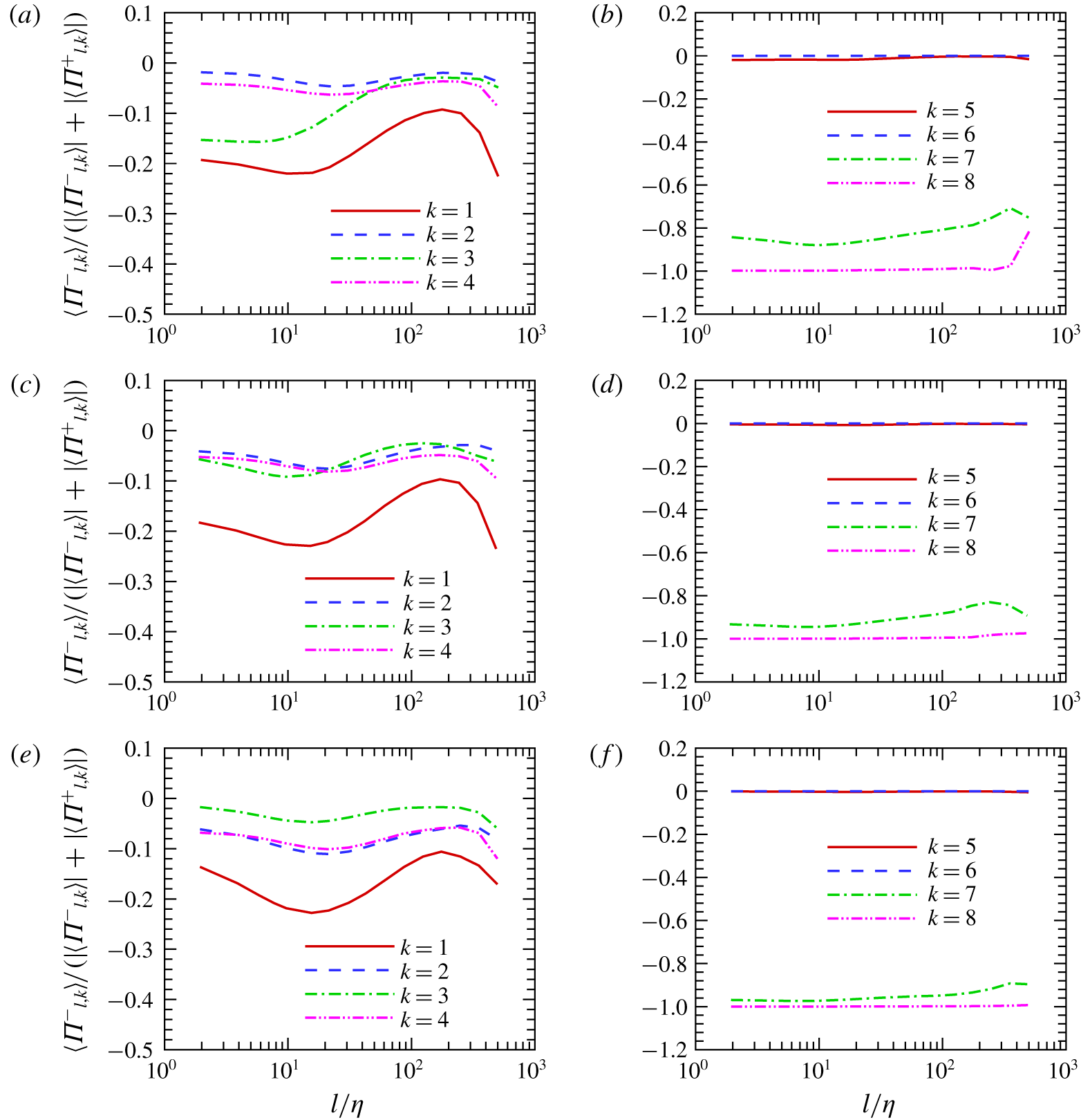
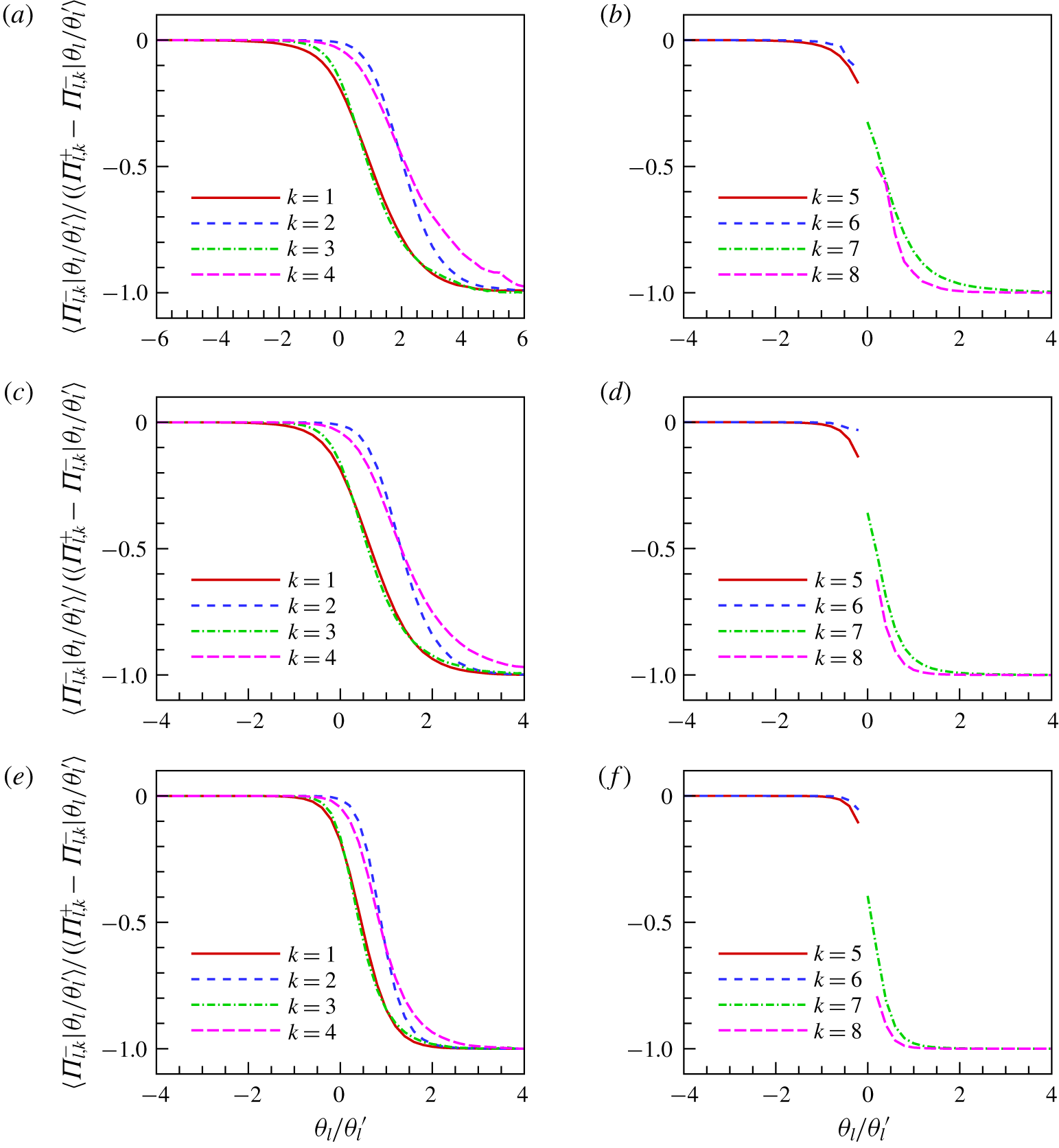
Normalized average of the negative component of SGS kinetic energy flux  $\langle \unicode[STIX]{x1D6F1}_{l,k}^{-}\rangle /(|\langle \unicode[STIX]{x1D6F1}_{l,k}^{-}\rangle |+|\langle \unicode[STIX]{x1D6F1}_{l,k}^{+}\rangle |)$ for the flow topology
 $S^{(k)}$. (a,b)
 $M_{t}=0.6$; (c,d)
 $M_{t}=0.8$; (e,f)
 $M_{t}=1.0$.

In order to investigate the effect of flow topology on the SGS kinetic energy backscatter, we define the contribution  $\unicode[STIX]{x1D6F1}_{l,k}^{-}$ from the type-
 $k$ (
 $S^{(k)}$) topology to the negative component of the SGS kinetic energy flux
 $\unicode[STIX]{x1D6F1}_{l}^{-}$ as follows:
 $\unicode[STIX]{x1D6F1}_{l,k}^{-}=\unicode[STIX]{x1D6F1}_{l}^{-}$ if the point is located in the
 $S^{(k)}$ topological region; otherwise, we set
 $\unicode[STIX]{x1D6F1}_{l,k}^{-}=0$. Similarly, we define the contribution
 $\unicode[STIX]{x1D6F1}_{l,k}^{+}$ from the type-
 $k$ (
 $S^{(k)}$) topology to the positive component of the SGS kinetic energy flux
 $\unicode[STIX]{x1D6F1}_{l}^{+}$ as follows:
 $\unicode[STIX]{x1D6F1}_{l,k}^{+}=\unicode[STIX]{x1D6F1}_{l}^{+}$ if the point is located in the
 $S^{(k)}$ topological region; otherwise, we set
 $\unicode[STIX]{x1D6F1}_{l,k}^{+}=0$. Therefore,
 $\unicode[STIX]{x1D6F1}_{l,k}=\unicode[STIX]{x1D6F1}_{l,k}^{-}+\unicode[STIX]{x1D6F1}_{l,k}^{+}$. We plot the normalized average of the negative component of the SGS kinetic energy flux
 $\langle \unicode[STIX]{x1D6F1}_{l,k}^{-}\rangle /(|\langle \unicode[STIX]{x1D6F1}_{l,k}^{-}\rangle |+|\langle \unicode[STIX]{x1D6F1}_{l,k}^{+}\rangle |)$ for the flow topology
 $S^{(k)}$ in figure 9. It is observed that the magnitude of
 $\langle \unicode[STIX]{x1D6F1}_{l,k}^{-}\rangle /(|\langle \unicode[STIX]{x1D6F1}_{l,k}^{-}\rangle |+|\langle \unicode[STIX]{x1D6F1}_{l,k}^{+}\rangle |)$ in the
 $S^{(1)}$ topological region is larger than those in the
 $S^{(2)}$,
 $S^{(3)}$ and
 $S^{(4)}$ topological regions, implying that the
 $S^{(1)}$ flow topology can induce more significant backscatter of kinetic energy than the
 $S^{(2)}$,
 $S^{(3)}$ and
 $S^{(4)}$ flow topologies. Moreover, the value of
 $\langle \unicode[STIX]{x1D6F1}_{l,k}^{-}\rangle /(|\langle \unicode[STIX]{x1D6F1}_{l,k}^{-}\rangle |+|\langle \unicode[STIX]{x1D6F1}_{l,k}^{+}\rangle |)$ is close to
 $0$ in the
 $S^{(5)}$ and
 $S^{(6)}$ topological regions, and is close to
 $-1$ in the
 $S^{(7)}$ and
 $S^{(8)}$ topological regions. These observations suggest that most kinetic energy transfer is from large scales to small scales in the
 $S^{(5)}$ and
 $S^{(6)}$ topological regions, while most kinetic energy transfer is from small scales to large scales in the
 $S^{(7)}$ and
 $S^{(8)}$ topological regions. In a previous study, we showed that the SGS backscatter of kinetic energy becomes more important as the turbulent Mach number becomes larger (Wang et al. Reference Wang, Wan, Chen and Chen2018a). Here, we infer that the increase of volume fraction of the
 $S^{(7)}$ topological regions with the increase of turbulent Mach number causes the increase of the SGS backscatter of kinetic energy.
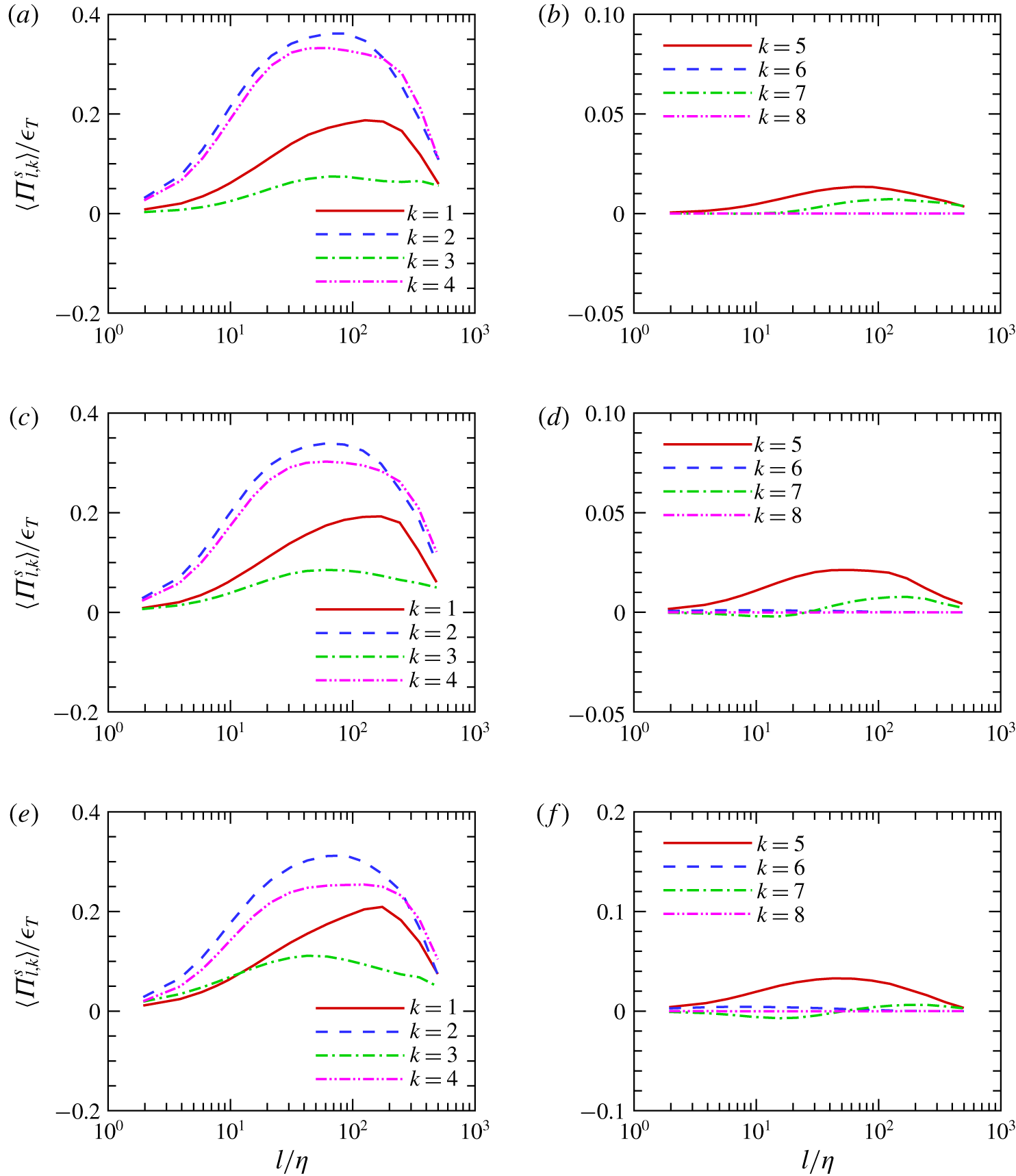
The average of contributions  $\langle \unicode[STIX]{x1D6F1}_{l,k}^{s}\rangle /\unicode[STIX]{x1D716}_{T}$ of various flow topologies
 $S^{(k)}$ to the solenoidal component of the normalized SGS kinetic energy flux
 $\unicode[STIX]{x1D6F1}_{l}^{s}/\unicode[STIX]{x1D716}_{T}$. (a,b)
 $M_{t}=0.6$; (c,d)
 $M_{t}=0.8$; (e,f)
 $M_{t}=1.0$.

Figure 10 shows the average contributions  $\langle \unicode[STIX]{x1D6F1}_{l,k}^{s}\rangle /\unicode[STIX]{x1D716}_{T}$, from various flow topological types, to the solenoidal component of the normalized SGS kinetic energy flux
 $\unicode[STIX]{x1D6F1}_{l}^{s}/\unicode[STIX]{x1D716}_{T}$ at the three turbulent Mach numbers. The average contributions of the
 $S^{(1)}$,
 $S^{(2)}$,
 $S^{(3)}$ and
 $S^{(4)}$ types to the solenoidal component of the normalized SGS kinetic energy flux are positive. The contributions from
 $S^{(2)}$ and
 $S^{(4)}$ to the solenoidal component of the normalized SGS kinetic energy flux are much larger than those from the other six topological types in the range of scales
 $10\leqslant l/\unicode[STIX]{x1D702}\leqslant 200$. The values of
 $\langle \unicode[STIX]{x1D6F1}_{l,2}^{s}\rangle /\unicode[STIX]{x1D716}_{T}$ and
 $\langle \unicode[STIX]{x1D6F1}_{l,4}^{s}\rangle /\unicode[STIX]{x1D716}_{T}$ decrease with the growth of the turbulent Mach number. The value of
 $\langle \unicode[STIX]{x1D6F1}_{l,2}^{s}\rangle /\unicode[STIX]{x1D716}_{T}$ is larger than that of
 $\langle \unicode[STIX]{x1D6F1}_{l,4}^{s}\rangle /\unicode[STIX]{x1D716}_{T}$ at scales
 $l/\unicode[STIX]{x1D702}\leqslant 100$, revealing the significant effect of the
 $S^{(2)}$ flow topology on the solenoidal component of the normalized SGS kinetic energy flux. The average contribution of the
 $S^{(5)}$ flow topology to the solenoidal component of the normalized SGS kinetic energy flux is positive, while the average contributions of the
 $S^{(6)}$,
 $S^{(7)}$ and
 $S^{(8)}$ flow topologies are negligibly small.
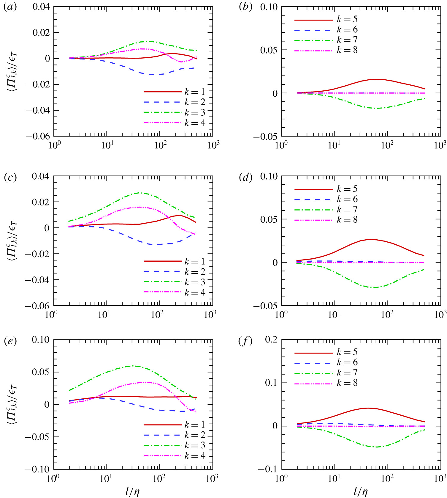
The average of contributions  $\langle \unicode[STIX]{x1D6F1}_{l,k}^{c}\rangle /\unicode[STIX]{x1D716}_{T}$ of various flow topologies
 $S^{(k)}$ to the compressible component of the normalized SGS kinetic energy flux
 $\unicode[STIX]{x1D6F1}_{l}^{c}/\unicode[STIX]{x1D716}_{T}$. (a–b)
 $M_{t}=0.6$; (c–d)
 $M_{t}=0.8$; (e–f)
 $M_{t}=1.0$.

Volume fractions  $V_{f}^{(k)}$ of various flow topologies
 $S^{(k)}$ conditioned on the normalized filtered velocity divergence for the filter width
 $l/\unicode[STIX]{x1D702}=16$. (a,b)
 $M_{t}=0.6$; (c,d)
 $M_{t}=0.8$; (e,f)
 $M_{t}=1.0$.

Figure 11 plots the average contributions  $\langle \unicode[STIX]{x1D6F1}_{l,k}^{c}\rangle /\unicode[STIX]{x1D716}_{T}$, from various flow topological types, to the compressible component of the normalized SGS kinetic energy flux
 $\unicode[STIX]{x1D6F1}_{l}^{c}/\unicode[STIX]{x1D716}_{T}$ at the three turbulent Mach numbers. The average contribution of the
 $S^{(3)}$ flow topology to the compressible component of the normalized SGS kinetic energy flux is positive, and increases significantly with the turbulent Mach number. The average contribution of the
 $S^{(4)}$ flow topology is positive at scales
 $l/\unicode[STIX]{x1D702}\leqslant 100$, and increases with the turbulent Mach number. In contrast, the average contribution of the
 $S^{(2)}$ flow topology is negative, implying that the
 $S^{(2)}$ flow topology makes a net contribution to the reverse SGS flux of the compressible component of the kinetic energy. The average contribution of the
 $S^{(1)}$ flow topology to the compressible component of the normalized SGS kinetic energy flux is always small at the three turbulent Mach numbers considered here.
The value of  $\langle \unicode[STIX]{x1D6F1}_{l,5}^{c}\rangle /\unicode[STIX]{x1D716}_{T}$ is positive, indicating that the flow topology
 $S^{(5)}$ makes a net contribution to the forward SGS flux of the compressible component of the kinetic energy. In contrast, the value of
 $\langle \unicode[STIX]{x1D6F1}_{l,7}^{c}\rangle /\unicode[STIX]{x1D716}_{T}$ is negative, demonstrating that the
 $S^{(7)}$ flow topology makes a net contribution to the reverse SGS flux of the compressible component of the kinetic energy. The magnitudes of
 $\langle \unicode[STIX]{x1D6F1}_{l,5}^{c}\rangle /\unicode[STIX]{x1D716}_{T}$ and
 $\langle \unicode[STIX]{x1D6F1}_{l,7}^{c}\rangle /\unicode[STIX]{x1D716}_{T}$ increase rapidly as the turbulent Mach number increases. The average contributions of the
 $S^{(6)}$ and
 $S^{(8)}$ flow topological types to the compressible component of the normalized SGS kinetic energy flux are negligibly small.
6.4 Effect of filtered velocity divergence on the kinetic energy flux in various flow topological regions
In order to clarify the effect of compression and expansion motions on the flow topology of the filtered velocity field, we calculate the conditionally averaged volume fractions of various flow topological types. Figure 12 plots the volume fractions  $V_{f}^{(k)}$ of various flow topological regions, conditioned on the normalized filtered velocity divergence for the filter width
 $l/\unicode[STIX]{x1D702}=16$ at the three turbulent Mach numbers. In the compression regions (
 $\unicode[STIX]{x1D703}_{l}<0$), as the magnitude of the filtered velocity divergence increases, the volume fraction of the
 $S^{(3)}$ flow topology increases rapidly, while the volume fractions of the
 $S^{(1)}$,
 $S^{(2)}$ and
 $S^{(4)}$ topological types decrease significantly. Moreover, the volume fraction of the
 $S^{(3)}$ flow topology increases with the increase of turbulent Mach number in the compression regions. The volume fraction of the
 $S^{(3)}$ topology is larger than those of the other seven flow topologies in the strong compression regions (
 $\unicode[STIX]{x1D703}_{l}/\unicode[STIX]{x1D703}_{l}^{\prime }<-3$) at relatively high turbulent Mach numbers
 $M_{t}=0.8,1.0$. The volume fraction of the
 $S^{(5)}$ flow topology is larger than
 $15\,\%$ in strong compression regions. The volume fraction of the
 $S^{(6)}$ flow topology increases as the magnitudes of the filtered velocity divergence and turbulent Mach number increase, in the strong compression regions (
 $\unicode[STIX]{x1D703}_{l}/\unicode[STIX]{x1D703}_{l}^{\prime }<-3$). Therefore, the strong compression regions are characterized by the stable-node/saddle/saddle topological structure.
In the expansion regions  $\unicode[STIX]{x1D703}_{l}>0$, the volume fractions of the
 $S^{(1)}$,
 $S^{(3)}$ and
 $S^{(4)}$ topological types decrease significantly with the increase of filtered velocity divergence. The volume fraction of the
 $S^{(2)}$ flow topology is larger than those of
 $S^{(1)}$,
 $S^{(3)}$ and
 $S^{(4)}$ in strong expansion regions (
 $\unicode[STIX]{x1D703}/\unicode[STIX]{x1D703}^{\prime }>3$). The volume fraction of the
 $S^{(7)}$ flow topology increases rapidly with the increase of the filtered velocity divergence and turbulent Mach number in the expansion regions, and is much larger than those of the other seven flow topologies in the strong expansion regions (
 $\unicode[STIX]{x1D703}_{l}/\unicode[STIX]{x1D703}_{l}^{\prime }>3$) at relatively high turbulent Mach numbers
 $M_{t}=0.8,1.0$. The volume fraction of flow topology
 $S^{(8)}$ increases as the filtered velocity divergence and turbulent Mach number increase, in the strong expansion regions (
 $\unicode[STIX]{x1D703}_{l}/\unicode[STIX]{x1D703}_{l}^{\prime }>3$). Therefore, the strong expansion regions are typically unstable foci with stretching in the direction normal to the focal plane.
The average of contributions  $\unicode[STIX]{x1D6F1}_{l,k}/\unicode[STIX]{x1D716}_{T}$ of various flow topologies
 $S^{(k)}$ to the normalized SGS kinetic energy flux
 $\unicode[STIX]{x1D6F1}_{l}/\unicode[STIX]{x1D716}_{T}$ conditioned on the normalized filtered velocity divergence for the filter width
 $l/\unicode[STIX]{x1D702}=16$. (a,b)
 $M_{t}=0.6$; (c,d)
 $M_{t}=0.8$; (e,f)
 $M_{t}=1.0$.

In order to address the compressibility effect on the SGS kinetic energy flux in various flow topological regions, we calculate the conditionally averaged contributions from various flow topological regions to the normalized SGS kinetic energy flux. Figure 13 depicts the average contributions  $\unicode[STIX]{x1D6F1}_{l,k}/\unicode[STIX]{x1D716}_{T}$ of various flow topological types to the normalized SGS kinetic energy flux
 $\unicode[STIX]{x1D6F1}_{l}/\unicode[STIX]{x1D716}_{T}$ conditioned on the normalized filtered velocity divergence for the filter width
 $l/\unicode[STIX]{x1D702}=16$ at the three turbulent Mach numbers. In the compression regions (
 $\unicode[STIX]{x1D703}_{l}<0$), the conditionally averaged values of
 $\unicode[STIX]{x1D6F1}_{l,1}$,
 $\unicode[STIX]{x1D6F1}_{l,2}$,
 $\unicode[STIX]{x1D6F1}_{l,3}$,
 $\unicode[STIX]{x1D6F1}_{l,4}$,
 $\unicode[STIX]{x1D6F1}_{l,5}$ and
 $\unicode[STIX]{x1D6F1}_{l,6}$ are positive, indicating that the corresponding flow topological types,
 $S^{(1)}$,
 $S^{(2)}$,
 $S^{(3)}$,
 $S^{(4)}$,
 $S^{(5)}$ and
 $S^{(6)}$, make a net contribution to the forward SGS flux of kinetic energy from large scales to small scales. Due to the effect of compressibility, the conditionally averaged values of
 $\unicode[STIX]{x1D6F1}_{l,3}$,
 $\unicode[STIX]{x1D6F1}_{l,5}$ and
 $\unicode[STIX]{x1D6F1}_{l,6}$ increase significantly with the increase of magnitudes of the filtered velocity divergence and turbulent Mach number. It is found that the contribution of the
 $S^{(3)}$ flow topology to the normalized SGS kinetic energy flux is much larger than those of the other seven flow topological types in the strong compression regions at high turbulent Mach numbers
 $M_{t}=0.8,1.0$.
In the expansion regions ( $\unicode[STIX]{x1D703}_{l}>0$), the magnitudes of the conditionally averaged values of
 $\unicode[STIX]{x1D6F1}_{l,3}$,
 $\unicode[STIX]{x1D6F1}_{l,4}$ and
 $\unicode[STIX]{x1D6F1}_{l,8}$ are smaller than those of
 $\unicode[STIX]{x1D6F1}_{l,1}$,
 $\unicode[STIX]{x1D6F1}_{l,2}$ and
 $\unicode[STIX]{x1D6F1}_{l,7}$. In the strong expansion regions (
 $\unicode[STIX]{x1D703}_{l}/\unicode[STIX]{x1D703}_{l}^{\prime }>3$), the conditionally averaged values of
 $\unicode[STIX]{x1D6F1}_{l,1}$,
 $\unicode[STIX]{x1D6F1}_{l,2}$ and
 $\unicode[STIX]{x1D6F1}_{l,7}$ are negative, implying that the
 $S^{(1)}$,
 $S^{(2)}$ and
 $S^{(7)}$ flow topological types make a net contribution to the reverse SGS flux of kinetic energy. It is shown that the contribution of the
 $S^{(7)}$ flow topology to the reverse SGS flux of kinetic energy is much larger than those of the other seven flow topological types in the strong expansion regions at high turbulent Mach numbers
 $M_{t}=0.8,1.0$.
Normalized conditional average of the negative component of SGS kinetic energy flux  $\langle \unicode[STIX]{x1D6F1}_{l,k}^{-}|\unicode[STIX]{x1D703}_{l}/\unicode[STIX]{x1D703}_{l}^{\prime }\rangle /\langle \unicode[STIX]{x1D6F1}_{l,k}^{+}-\unicode[STIX]{x1D6F1}_{l,k}^{-}|\unicode[STIX]{x1D703}_{l}/\unicode[STIX]{x1D703}_{l}^{\prime }\rangle$ in the flow topology
 $S^{(k)}$ for the filter width
 $l/\unicode[STIX]{x1D702}=16$. (a,b)
 $M_{t}=0.6$; (c,d)
 $M_{t}=0.8$; (e,f)
 $M_{t}=1.0$.

We show the normalized conditional average value of negative component of SGS kinetic energy flux  $\langle \unicode[STIX]{x1D6F1}_{l,k}^{-}|\unicode[STIX]{x1D703}_{l}/\unicode[STIX]{x1D703}_{l}^{\prime }\rangle /\langle \unicode[STIX]{x1D6F1}_{l,k}^{+}-\unicode[STIX]{x1D6F1}_{l,k}^{-}|\unicode[STIX]{x1D703}_{l}/\unicode[STIX]{x1D703}_{l}^{\prime }\rangle$ in the flow topology
 $S^{(k)}$ for the filter width
 $l/\unicode[STIX]{x1D702}=16$ in figure 14. The conditional average value at
 $k=5,6$ is plotted only for
 $\unicode[STIX]{x1D703}_{l}/\unicode[STIX]{x1D703}_{l}^{\prime }<0$ since the
 $S^{(5)}$ and
 $S^{(6)}$ flow topologies only exist in compression regions. Similarly, the conditional average value at
 $k=7,8$ is plotted only for
 $\unicode[STIX]{x1D703}_{l}/\unicode[STIX]{x1D703}_{l}^{\prime }>0$. We find that the value of
 $\langle \unicode[STIX]{x1D6F1}_{l,k}^{-}|\unicode[STIX]{x1D703}_{l}/\unicode[STIX]{x1D703}_{l}^{\prime }\rangle /\langle \unicode[STIX]{x1D6F1}_{l,k}^{+}-\unicode[STIX]{x1D6F1}_{l,k}^{-}|\unicode[STIX]{x1D703}_{l}/\unicode[STIX]{x1D703}_{l}^{\prime }\rangle$ is always close to
 $0$ for
 $\unicode[STIX]{x1D703}_{l}/\unicode[STIX]{x1D703}_{l}^{\prime }\leqslant -2.0$, indicating that most kinetic energy transfer is from large scales to small scales in strong compression regions. We also observe that the value of
 $\langle \unicode[STIX]{x1D6F1}_{l,k}^{-}|\unicode[STIX]{x1D703}_{l}/\unicode[STIX]{x1D703}_{l}^{\prime }\rangle /\langle \unicode[STIX]{x1D6F1}_{l,k}^{+}-\unicode[STIX]{x1D6F1}_{l,k}^{-}|\unicode[STIX]{x1D703}_{l}/\unicode[STIX]{x1D703}_{l}^{\prime }\rangle$ tends to be
 $-1$ as
 $\unicode[STIX]{x1D703}_{l}/\unicode[STIX]{x1D703}_{l}^{\prime }$ becomes larger in strong expansion regions. Thus, the effect of strong expansion motions on the SGS kinetic energy flux is opposite to that of strong compression motions. The effects of both expansion and compression motions become more significant with the increase of turbulent Mach number. It is worth noting that in expansion regions, the
 $S^{(1)}$ and
 $S^{(3)}$ flow topologies can cause more significant backscatter of kinetic energy than the
 $S^{(2)}$ and
 $S^{(4)}$ flow topologies.
Average of  $\unicode[STIX]{x1D709}_{l}$ conditioned on the normalized velocity divergence and the flow topology
 $S^{(k)}$ for the filter width
 $l/\unicode[STIX]{x1D702}=16$. (a,b)
 $M_{t}=0.6$; (c,d)
 $M_{t}=0.8$; (e,f)
 $M_{t}=1.0$.

In order to investigate the relation between the large-scale strain and the SGS stress, we introduce the following geometrical variable for the SGS kinetic energy flux:
 $$\begin{eqnarray}\unicode[STIX]{x1D709}_{l}=\frac{\widetilde{\unicode[STIX]{x1D70F}}_{ij}\widetilde{\unicode[STIX]{x1D61A}}_{ij}}{|\widetilde{\unicode[STIX]{x1D749}}||\widetilde{\unicode[STIX]{x1D64E}}|},\end{eqnarray}$$
where  $|\widetilde{\unicode[STIX]{x1D749}}|=\sqrt{\widetilde{\unicode[STIX]{x1D70F}}_{ij}\widetilde{\unicode[STIX]{x1D70F}}_{ij}}$ and
 $|\widetilde{\unicode[STIX]{x1D64E}}|=\sqrt{\widetilde{\unicode[STIX]{x1D61A}}_{ij}\widetilde{\unicode[STIX]{x1D61A}}_{ij}}$. We depict the average value of
 $\unicode[STIX]{x1D709}_{l}$ conditioned on the normalized velocity divergence and the flow topology
 $S^{(k)}$ for the filter width
 $l/\unicode[STIX]{x1D702}=16$ in figure 15. The irregular fluctuations of the conditional average values at
 $k=3,4$ for large positive normalized velocity divergence are due to the lack of data samples, since the conditional volume fractions of the
 $S^{(3)}$ and
 $S^{(4)}$ flow topologies are very small for large positive normalized velocity divergence. We show that the conditional average of
 $\unicode[STIX]{x1D709}_{l}$ is close to
 $-1$ for
 $\unicode[STIX]{x1D703}_{l}/\unicode[STIX]{x1D703}_{l}^{\prime }\leqslant -4.0$, indicating the antiparallel alignment between the large-scale strain and the SGS stress in strong compression regions. Thus, the SGS kinetic energy flux is maximized by the antiparallel alignment between the large-scale strain and the SGS stress in strong compression regions. We also find that the conditional average of
 $\unicode[STIX]{x1D709}_{l}$ is larger than
 $0.5$ for
 $\unicode[STIX]{x1D703}_{l}/\unicode[STIX]{x1D703}_{l}^{\prime }\geqslant 4.0$, giving rise to the reverse SGS flux of kinetic energy from small scales to large scales in strong expansion regions. The conditional average of
 $\unicode[STIX]{x1D709}_{l}$ exhibits qualitatively similar behaviours in different flow topologies. The effect of compression and expansion motions on the conditional average of
 $\unicode[STIX]{x1D709}_{l}$ is more significant for
 $S^{(6)}$ and
 $S^{(8)}$ flow topologies, as compared to other six flow topologies.
The average contributions  $\unicode[STIX]{x1D6F1}_{l,k}^{s}/\unicode[STIX]{x1D716}_{T}$ of various flow topologies
 $S^{(k)}$ to the solenoidal component of the normalized SGS kinetic energy flux
 $\unicode[STIX]{x1D6F1}_{l}^{s}/\unicode[STIX]{x1D716}_{T}$ conditioned on the normalized filtered velocity divergence for the filter width
 $l/\unicode[STIX]{x1D702}=16$. (a,b)
 $M_{t}=0.6$; (c,d)
 $M_{t}=0.8$; (e,f)
 $M_{t}=1.0$.

Figure 16 shows the average contributions  $\unicode[STIX]{x1D6F1}_{l,k}^{s}/\unicode[STIX]{x1D716}_{T}$, from various flow topological types, to the solenoidal component of the normalized SGS kinetic energy flux
 $\unicode[STIX]{x1D6F1}_{l}^{s}/\unicode[STIX]{x1D716}_{T}$, conditioned on the normalized filtered velocity divergence for the filter width
 $l/\unicode[STIX]{x1D702}=16$ at the three turbulent Mach numbers. The behaviours of conditionally averaged
 $\unicode[STIX]{x1D6F1}_{l,k}^{s}$ are quite similar to those of
 $\unicode[STIX]{x1D6F1}_{l,k}$. In the compression regions (
 $\unicode[STIX]{x1D703}_{l}<0$), the conditionally averaged values of
 $\unicode[STIX]{x1D6F1}_{l,1}^{s}$,
 $\unicode[STIX]{x1D6F1}_{l,2}^{s}$,
 $\unicode[STIX]{x1D6F1}_{l,3}^{s}$,
 $\unicode[STIX]{x1D6F1}_{l,4}^{s}$,
 $\unicode[STIX]{x1D6F1}_{l,5}^{s}$ and
 $\unicode[STIX]{x1D6F1}_{l,6}^{s}$ are positive. The conditionally averaged values,
 $\unicode[STIX]{x1D6F1}_{l,3}^{s}$,
 $\unicode[STIX]{x1D6F1}_{l,5}^{s}$ and
 $\unicode[STIX]{x1D6F1}_{l,6}^{s}$, increase significantly as the magnitudes of the filtered velocity divergence and turbulent Mach number increase. The contribution of the
 $S^{(3)}$ flow topology to the solenoidal component of normalized SGS kinetic energy flux is much larger than those of the other seven flow topological types in the strong compression regions at high turbulent Mach numbers
 $M_{t}=0.8,1.0$. In the strong expansion regions (
 $\unicode[STIX]{x1D703}_{l}/\unicode[STIX]{x1D703}_{l}^{\prime }>3$), the conditionally averaged values of
 $\unicode[STIX]{x1D6F1}_{l,1}^{s}$,
 $\unicode[STIX]{x1D6F1}_{l,2}^{s}$ and
 $\unicode[STIX]{x1D6F1}_{l,7}^{s}$ are negative. The contribution of the
 $S^{(7)}$ flow topology to the reverse SGS flux of the solenoidal component of kinetic energy is much larger than those of the other seven flow topologies in strong expansion regions at high turbulent Mach numbers
 $M_{t}=0.8,1.0$.
The average contributions  $\unicode[STIX]{x1D6F1}_{l,k}^{c}/\unicode[STIX]{x1D716}_{T}$ of various flow topologies
 $S^{(k)}$ to the compressible component of normalized SGS kinetic energy flux
 $\unicode[STIX]{x1D6F1}_{l}^{c}/\unicode[STIX]{x1D716}_{T}$ conditioned on the normalized filtered velocity divergence for the filter width
 $l/\unicode[STIX]{x1D702}=16$. (a,b)
 $M_{t}=0.6$; (c,d)
 $M_{t}=0.8$; (e,f)
 $M_{t}=1.0$.

Figure 17 shows the average contributions  $\unicode[STIX]{x1D6F1}_{l,k}^{c}/\unicode[STIX]{x1D716}_{T}$, from various flow topological regions, to the compressible component of the normalized SGS kinetic energy flux
 $\unicode[STIX]{x1D6F1}_{l}^{c}/\unicode[STIX]{x1D716}_{T}$, conditioned on the normalized filtered velocity divergence for the filter width
 $l/\unicode[STIX]{x1D702}=16$. The behaviours of conditionally averaged
 $\unicode[STIX]{x1D6F1}_{l,k}^{c}$ are quite similar to those of
 $\unicode[STIX]{x1D6F1}_{l,k}$ and
 $\unicode[STIX]{x1D6F1}_{l,k}^{s}$. In the strong compression regions, the contribution of the
 $S^{(3)}$ flow topology to the compressible component of the normalized SGS kinetic energy flux is predominant over the other seven flow topologies at high turbulent Mach numbers
 $M_{t}=0.8,1.0$. In the strong expansion regions, the contribution of the
 $S^{(7)}$ flow topology to the reverse SGS flux of the compressible component of kinetic energy is predominant over the other seven flow topologies at high turbulent Mach numbers
 $M_{t}=0.8,1.0$.
Volume fractions  $V_{f}^{(3)}$ and
 $V_{f}^{(7)}$ of flow topologies
 $S^{(3)}$ and
 $S^{(7)}$ conditioned on the normalized filtered velocity divergence. (a,b)
 $M_{t}=0.8$; (c,d)
 $M_{t}=1.0$.

Due to the importance of the  $S^{(3)}$ and
 $S^{(7)}$ topological types in the strong compression and strong expansion regions, we plot the volume fractions
 $V_{f}^{(3)}$ and
 $V_{f}^{(7)}$, conditioned on the normalized filtered velocity divergence, for the filter widths
 $l/\unicode[STIX]{x1D702}=16$, 24, 32, 48, 64 in figure 18. The volume fraction
 $V_{f}^{(3)}$ increases rapidly with the increase of magnitude of the filtered velocity divergence in the compression regions
 $\unicode[STIX]{x1D703}_{l}/\unicode[STIX]{x1D703}_{l}^{\prime }\leqslant 0$, and is larger than
 $30\,\%$ for
 $\unicode[STIX]{x1D703}_{l}/\unicode[STIX]{x1D703}_{l}^{\prime }\leqslant -4$ at turbulent Mach numbers
 $M_{t}=0.8,1.0$. The volume fraction
 $V_{f}^{(7)}$ increases rapidly with the increase of filtered velocity divergence in the expansion regions, and is larger than
 $40\,\%$ for
 $\unicode[STIX]{x1D703}_{l}/\unicode[STIX]{x1D703}_{l}^{\prime }\geqslant 4$ at turbulent Mach numbers
 $M_{t}=0.8,1.0$. Due to the lack of samples, the data are quite scattered when the magnitude of the filtered velocity divergence and the filter width are large. It is shown that numerical results for the conditionally averaged volume fractions nearly collapse onto one another for different filter widths when
 $|\unicode[STIX]{x1D703}_{l}/\unicode[STIX]{x1D703}_{l}^{\prime }|\leqslant 2$, implying that the dependency of the conditionally averaged volume fractions on the filter width is quite weak. As the filter width
 $l/\unicode[STIX]{x1D702}$ increases from
 $16$ to
 $64$,
 $V_{f}^{(3)}$ decreases slightly in strong compression regions (
 $\unicode[STIX]{x1D703}_{l}/\unicode[STIX]{x1D703}_{l}^{\prime }\leqslant -3$), while
 $V_{f}^{(7)}$ increases in the strong expansion regions (
 $\unicode[STIX]{x1D703}_{l}/\unicode[STIX]{x1D703}_{l}^{\prime }\geqslant 3$). According to the Kolmogorov theory in the inertial range of turbulence, the flow dynamics of the inertial range is nearly independent of both the external scale and dissipation scale, and exhibits self-similarity properties, which is statistically signified by the power-law scaling behaviours of the velocity spectrum and velocity structure functions. Here, we show that the statistical relations between the filtered velocity divergence and the volume fractions
 $V_{f}^{(3)}$ and
 $V_{f}^{(7)}$ are also nearly independent of filter width, and exhibit nearly self-similarity properties in the inertial range. We infer that the Kolmogorov turbulence theory of the inertial range can be extended to describe a variety of statistical properties of compressible turbulence, and such observations may be used to simplify the development of SGS models for LES of compressible turbulence. The slight dependence of volume fractions
 $V_{f}^{(3)}$ and
 $V_{f}^{(7)}$ on the filter width in strong compression regions and strong expansion regions can be attributed to the intermittency of turbulence.
The average of contributions  $\unicode[STIX]{x1D6F1}_{l,3}/\unicode[STIX]{x1D716}_{T}$ and
 $\unicode[STIX]{x1D6F1}_{l,7}/\unicode[STIX]{x1D716}_{T}$ of flow topologies
 $S^{(3)}$ and
 $S^{(7)}$ to the normalized SGS kinetic energy flux
 $\unicode[STIX]{x1D6F1}_{l}/\unicode[STIX]{x1D716}_{T}$ conditioned on the normalized filtered velocity divergence. (a,b)
 $M_{t}=0.8$; (c,d)
 $M_{t}=1.0$. Here,
 $\unicode[STIX]{x1D6FC}_{3}=0.1,0.23$ for turbulent Mach numbers
 $M_{t}=0.8,1.0$, respectively;
 $\unicode[STIX]{x1D6FC}_{7}=0.1,0.18$ for turbulent Mach numbers
 $M_{t}=0.8,1.0$, respectively.

Figure 19 plots the averaged  $\unicode[STIX]{x1D6F1}_{l,3}/\unicode[STIX]{x1D716}_{T}$ and
 $\unicode[STIX]{x1D6F1}_{l,7}/\unicode[STIX]{x1D716}_{T}$, from the
 $S^{(3)}$ and
 $S^{(7)}$ flow topological types, to the normalized SGS kinetic energy flux
 $\unicode[STIX]{x1D6F1}_{l}/\unicode[STIX]{x1D716}_{T}$ conditioned on the normalized filtered velocity divergence, for the filter widths
 $l/\unicode[STIX]{x1D702}=16,24,32,48,64$. The conditionally averaged values of
 $\unicode[STIX]{x1D6F1}_{l,3}/\unicode[STIX]{x1D716}_{T}$ and
 $\unicode[STIX]{x1D6F1}_{l,7}/\unicode[STIX]{x1D716}_{T}$ are nearly independent of filter width
 $l/\unicode[STIX]{x1D702}$, for
 $16\leqslant l/\unicode[STIX]{x1D702}\leqslant 64$ at
 $M_{t}=0.8,1.0$. When the magnitude of the filtered velocity divergence
 $\unicode[STIX]{x1D703}_{l}/\unicode[STIX]{x1D703}_{l}^{\prime }$ and the filter width
 $l/\unicode[STIX]{x1D702}$ is large, the data are quite scattered due to the lack of samples. We propose simple algebraic relations for the conditionally averaged
 $\unicode[STIX]{x1D6F1}_{l,3}/\unicode[STIX]{x1D716}_{T}$ in the compression regions (
 $\unicode[STIX]{x1D703}_{l}\leqslant 0$) and
 $\unicode[STIX]{x1D6F1}_{l,7}/\unicode[STIX]{x1D716}_{T}$ in the expansion regions (
 $\unicode[STIX]{x1D703}_{l}\geqslant 0$),
 $$\begin{eqnarray}\langle \unicode[STIX]{x1D6F1}_{l,3}/\unicode[STIX]{x1D716}_{T}|\unicode[STIX]{x1D703}_{l}/\unicode[STIX]{x1D703}_{l}^{\prime }\rangle =\unicode[STIX]{x1D6FC}_{3}(\unicode[STIX]{x1D703}_{l}/\unicode[STIX]{x1D703}_{l}^{\prime })^{2},\quad \unicode[STIX]{x1D703}_{l}\leqslant 0,\end{eqnarray}$$
where  $\unicode[STIX]{x1D6FC}_{3}=0.1,0.23$ for turbulent Mach numbers
 $M_{t}=0.8,1.0$, respectively. Here
 $$\begin{eqnarray}\langle \unicode[STIX]{x1D6F1}_{l,7}/\unicode[STIX]{x1D716}_{T}|\unicode[STIX]{x1D703}_{l}/\unicode[STIX]{x1D703}_{l}^{\prime }\rangle =-\unicode[STIX]{x1D6FC}_{7}(\unicode[STIX]{x1D703}_{l}/\unicode[STIX]{x1D703}_{l}^{\prime })^{2},\quad \unicode[STIX]{x1D703}_{l}\geqslant 0,\end{eqnarray}$$
where  $\unicode[STIX]{x1D6FC}_{7}=0.1,0.18$ for turbulent Mach numbers
 $M_{t}=0.8,1.0$, respectively. The numerical results for the conditionally averaged
 $\unicode[STIX]{x1D6F1}_{l,3}/\unicode[STIX]{x1D716}_{T}$ and
 $\unicode[STIX]{x1D6F1}_{l,7}/\unicode[STIX]{x1D716}_{T}$ are in good agreement with (6.4) and (6.5). The algebraic relations indicate that strong compression motions induce direct SGS flux of kinetic energy from large scales to small scales in the
 $S^{(3)}$ flow topology regions, while strong expansion motions lead to reverse SGS flux of kinetic energy from small scales to large scales in the
 $S^{(7)}$ flow topology regions. In addition, the magnitude of the SGS flux of kinetic energy increases linearly with the square of the filtered velocity divergence, demonstrating the significant effect of compressibility on the SGS flux of kinetic energy in the
 $S^{(3)}$ and
 $S^{(7)}$ flow topology regions. Previous studies showed that strong compression motions can be identified in sheet-like shocklets (Wang et al. Reference Wang, Shi, Wang, Xiao, He and Chen2011, Reference Wang, Gotoh and Watanabe2017b), where kinetic energy is dissipated by viscosity quickly and the viscous dissipation of kinetic energy is proportional to the square of the velocity divergence. Shocklet regions can be viewed as kinetic energy sinks which absorb kinetic energy persistently from large-scale flows through direct cascade of kinetic energy (Wang et al. Reference Wang, Yang, Shi, Xiao, He and Chen2013, Reference Wang, Wan, Chen and Chen2018a). The magnitude of the kinetic energy flux in the inertial range should be proportional to the local average of the dissipation rate of the shocklet at the scale of the filter width, based on the assumption of the locality of kinetic energy transfer (Aluie Reference Aluie2011). Thus, the conditionally averaged SGS kinetic energy flux is proportional to the square of the filtered velocity divergence in strong compression regions (Wang et al. Reference Wang, Yang, Shi, Xiao, He and Chen2013, Reference Wang, Wan, Chen and Chen2018a). In strong expansion regions with the
 $S^{(7)}$ flow topology, kinetic energy transfers from small scales to large scale, which is opposite to the situation of strong compression regions with the
 $S^{(3)}$ flow topology. Moreover, the magnitude of the conditionally averaged SGS kinetic energy flux also increases linearly with the square of the filtered velocity divergence, demonstrating the quantitative similarity between the effects of strong expansion motions and compression motions on the kinetic energy transfer. The observation suggests that strong expansion regions with the
 $S^{(7)}$ flow topology can be viewed as kinetic energy sources which inject kinetic energy to large-scale flows through reverse cascade of kinetic energy.
According to the usual kinetic energy cascade scenario, in the statistical sense, the kinetic energy is injected at the integral length scale, transferred from large scales to small scales and dissipated at the Kolmogorov length scale. In the inertial range between the integral length scale and the Kolmogorov length scale, the SGS flux of kinetic energy exhibits some scale-invariant properties: (i) the spatial average of SGS flux is nearly constant; (ii) the average of SGS flux conditioned on the filtered velocity divergence is independent of filter scales (Wang et al. Reference Wang, Yang, Shi, Xiao, He and Chen2013, Reference Wang, Wan, Chen and Chen2018a). Here, it is shown that the average values of SGS fluxes  $\unicode[STIX]{x1D6F1}_{l,3}/\unicode[STIX]{x1D716}_{T}$ and
 $\unicode[STIX]{x1D6F1}_{l,7}/\unicode[STIX]{x1D716}_{T}$, conditioned on the filtered velocity divergence, are also nearly scale invariant in the strong compression or expansion regions during the kinetic energy cascade in solenoidally forced compressible isotropic turbulence. We believe that scale-invariant properties are quite general in turbulence regardless of the complex effects of compression motions and expansion motions, which are critical to developing efficient SGS models for LES of compressible turbulence (Meneveau & Katz Reference Meneveau and Katz2000).
A previous study showed that the conditionally averaged SGS kinetic energy flux is proportional to  $\unicode[STIX]{x1D703}_{l}^{1.2}$ in the strong expansion regions at turbulent Mach numbers
 $M_{t}=0.6,0.8,1.0$ in solenoidally forced compressible isotropic turbulence (Wang et al. Reference Wang, Wan, Chen and Chen2018a). Here, it is found that the conditionally averaged SGS kinetic energy flux
 $\unicode[STIX]{x1D6F1}_{l,7}/\unicode[STIX]{x1D716}_{T}$ from the
 $S^{(7)}$ flow topology is proportional to
 $\unicode[STIX]{x1D703}_{l}^{2}$ in the strong expansion regions at turbulent Mach numbers
 $M_{t}=0.8,1.0$, demonstrating the strong effect of compressibility on the inverse SGS flux of kinetic energy in the
 $S^{(7)}$ flow topology. We note that the compressibility effect is weakened by other flow topological types, leading to the
 $\unicode[STIX]{x1D703}_{l}^{1.2}$ scaling of overall SGS kinetic energy flux in the strong expansion regions.
Iso-surfaces of filtered velocity divergence for  $l/\unicode[STIX]{x1D702}=16,32$ at
 $M_{t}=1.0$. (a)
 $\unicode[STIX]{x1D703}_{l}/\unicode[STIX]{x1D703}_{l}^{\prime }=-3.0$ and
 $l/\unicode[STIX]{x1D702}=16$; (b)
 $\unicode[STIX]{x1D703}_{l}/\unicode[STIX]{x1D703}_{l}^{\prime }=2.0$ and
 $l/\unicode[STIX]{x1D702}=16$; (c)
 $\unicode[STIX]{x1D703}_{l}/\unicode[STIX]{x1D703}_{l}^{\prime }=-3.0$ and
 $l/\unicode[STIX]{x1D702}=32$; (d)
 $\unicode[STIX]{x1D703}_{l}/\unicode[STIX]{x1D703}_{l}^{\prime }=2.0$ and
 $l/\unicode[STIX]{x1D702}=32$.

Figure 20 displays the iso-surfaces of filtered velocity divergence for  $l/\unicode[STIX]{x1D702}=16,32$ at
 $M_{t}=1.0$. The iso-surfaces are coloured based on the normalized flux of kinetic energy
 $\unicode[STIX]{x1D6F1}_{l}/\unicode[STIX]{x1D6F1}_{l}^{\prime }$, where
 $\unicode[STIX]{x1D6F1}_{l}^{\prime }$ denotes the r.m.s. value of kinetic energy flux
 $\unicode[STIX]{x1D6F1}_{l}$. The iso-surfaces of
 $\unicode[STIX]{x1D703}_{l}/\unicode[STIX]{x1D703}_{l}^{\prime }=-3.0$ associated with strong compression motions are sheet-like, which can be attributed to the generation of shocklets at
 $M_{t}=1.0$. The kinetic energy flux is positive on the iso-surfaces of
 $\unicode[STIX]{x1D703}_{l}/\unicode[STIX]{x1D703}_{l}^{\prime }=-3.0$, suggesting that strong compression motions cause the direct flux of kinetic energy from large scales to small scales. The iso-surfaces of
 $\unicode[STIX]{x1D703}_{l}/\unicode[STIX]{x1D703}_{l}^{\prime }=2.0$, associated with strong expansion motions, are blob-like, with smaller length scales as compared to iso-surfaces of
 $\unicode[STIX]{x1D703}_{l}/\unicode[STIX]{x1D703}_{l}^{\prime }=-3.0$. Moreover, the spatial distributions of iso-surfaces of
 $\unicode[STIX]{x1D703}_{l}/\unicode[STIX]{x1D703}_{l}^{\prime }=2.0$ are more uniform than those of iso-surfaces of
 $\unicode[STIX]{x1D703}_{l}/\unicode[STIX]{x1D703}_{l}^{\prime }=-3.0$. The kinetic energy flux is negative on the iso-surfaces of
 $\unicode[STIX]{x1D703}_{l}/\unicode[STIX]{x1D703}_{l}^{\prime }=2.0$, indicating that strong expansion motions induce the reverse flux of kinetic energy. It is also observed that the iso-surfaces of
 $\unicode[STIX]{x1D703}_{l}/\unicode[STIX]{x1D703}_{l}^{\prime }=-3.0$ and
 $\unicode[STIX]{x1D703}_{l}/\unicode[STIX]{x1D703}_{l}^{\prime }=2.0$ exhibit geometrical self-similarities at different filter widths
 $l/\unicode[STIX]{x1D702}=16,32$. As the filter width increases, iso-surfaces of
 $\unicode[STIX]{x1D703}_{l}/\unicode[STIX]{x1D703}_{l}^{\prime }=-3.0$ have a larger thickness but with almost the same spanwise scale, while iso-surfaces of
 $\unicode[STIX]{x1D703}_{l}/\unicode[STIX]{x1D703}_{l}^{\prime }=2.0$ show a larger diameter. In a previous study, we plotted the iso-surfaces of the normalized flux of kinetic energy
 $\unicode[STIX]{x1D6F1}_{l}/\unicode[STIX]{x1D6F1}_{l}^{\prime }$ (Wang et al. Reference Wang, Wan, Chen and Chen2018a). It is worth noting that the iso-surfaces of
 $\unicode[STIX]{x1D6F1}_{l}/\unicode[STIX]{x1D6F1}_{l}^{\prime }=2.0$ are similar to the iso-surfaces of
 $\unicode[STIX]{x1D703}_{l}/\unicode[STIX]{x1D703}_{l}^{\prime }=-3.0$, while the iso-surfaces of
 $\unicode[STIX]{x1D6F1}_{l}/\unicode[STIX]{x1D6F1}_{l}^{\prime }=-0.5$ are similar to the iso-surfaces of
 $\unicode[STIX]{x1D703}_{l}/\unicode[STIX]{x1D703}_{l}^{\prime }=2.0$. Thus, strong compression motions and expansion motions can give rise to the different spatial patterns of locally direct or reverse transfer of kinetic energy. Moreover, the scale-invariant properties of kinetic energy flux can be related to the geometrical self-similarities of strong compression motions and expansion motions.
The average of contributions  $\unicode[STIX]{x1D6F1}_{l,3}^{s}/\unicode[STIX]{x1D716}_{T}$ and
 $\unicode[STIX]{x1D6F1}_{l,7}^{s}/\unicode[STIX]{x1D716}_{T}$ of flow topologies
 $S^{(3)}$ and
 $S^{(7)}$ to the solenoidal component of the normalized SGS kinetic energy flux
 $\unicode[STIX]{x1D6F1}_{l}^{s}/\unicode[STIX]{x1D716}_{T}$ conditioned on the normalized filtered velocity divergence. (a,b)
 $M_{t}=0.8$; (c,d)
 $M_{t}=1.0$. Here,
 $\unicode[STIX]{x1D6FC}_{3}^{s}=0.052,0.11$ for turbulent Mach numbers
 $M_{t}=0.8,1.0$, respectively;
 $\unicode[STIX]{x1D6FC}_{7}^{s}=0.042,0.075$ for turbulent Mach numbers
 $M_{t}=0.8,1.0$, respectively.

In figure 21, we show the averaged  $\unicode[STIX]{x1D6F1}_{l,3}^{s}/\unicode[STIX]{x1D716}_{T}$ and
 $\unicode[STIX]{x1D6F1}_{l,7}^{s}/\unicode[STIX]{x1D716}_{T}$, from the
 $S^{(3)}$ and
 $S^{(7)}$ flow topological types, to the solenoidal component of the normalized SGS kinetic energy flux
 $\unicode[STIX]{x1D6F1}_{l}^{s}/\unicode[STIX]{x1D716}_{T}$, conditioned on the normalized filtered velocity divergence, for the filter widths
 $l/\unicode[STIX]{x1D702}=16,24,32,48,64$. Similar to the conditionally averaged values of
 $\unicode[STIX]{x1D6F1}_{l,3}/\unicode[STIX]{x1D716}_{T}$ and
 $\unicode[STIX]{x1D6F1}_{l,7}/\unicode[STIX]{x1D716}_{T}$, the conditionally averaged values of
 $\unicode[STIX]{x1D6F1}_{l,3}^{s}/\unicode[STIX]{x1D716}_{T}$ and
 $\unicode[STIX]{x1D6F1}_{l,7}^{s}/\unicode[STIX]{x1D716}_{T}$ are nearly independent of filter width
 $l/\unicode[STIX]{x1D702}$. In addition, similar algebraic relations for the conditionally averaged
 $\unicode[STIX]{x1D6F1}_{l,3}^{s}/\unicode[STIX]{x1D716}_{T}$ in the compression regions (
 $\unicode[STIX]{x1D703}_{l}\leqslant 0$) and
 $\unicode[STIX]{x1D6F1}_{l,7}^{s}/\unicode[STIX]{x1D716}_{T}$ in the expansion regions (
 $\unicode[STIX]{x1D703}_{l}\geqslant 0$) can be introduced:
 $$\begin{eqnarray}\langle \unicode[STIX]{x1D6F1}_{l,3}^{s}/\unicode[STIX]{x1D716}_{T}|\unicode[STIX]{x1D703}_{l}/\unicode[STIX]{x1D703}_{l}^{\prime }\rangle =\unicode[STIX]{x1D6FC}_{3}^{s}(\unicode[STIX]{x1D703}_{l}/\unicode[STIX]{x1D703}_{l}^{\prime })^{2},\quad \unicode[STIX]{x1D703}_{l}\leqslant 0,\end{eqnarray}$$
where  $\unicode[STIX]{x1D6FC}_{3}^{s}=0.052,0.11$ for turbulent Mach numbers
 $M_{t}=0.8,1.0$, respectively. Here
 $$\begin{eqnarray}\langle \unicode[STIX]{x1D6F1}_{l,7}^{s}/\unicode[STIX]{x1D716}_{T}|\unicode[STIX]{x1D703}_{l}/\unicode[STIX]{x1D703}_{l}^{\prime }\rangle =-\unicode[STIX]{x1D6FC}_{7}^{s}(\unicode[STIX]{x1D703}_{l}/\unicode[STIX]{x1D703}_{l}^{\prime })^{2},\quad \unicode[STIX]{x1D703}_{l}\geqslant 0,\end{eqnarray}$$
where  $\unicode[STIX]{x1D6FC}_{7}^{s}=0.042,0.075$ for turbulent Mach numbers
 $M_{t}=0.8,1.0$, respectively. We find that the numerical results are in good agreement with (6.6) and (6.7), as shown in figure 21. The algebraic relations suggest the strong influences of compressible motions on the inter-scale transfer of the solenoidal component of kinetic energy, through the couplings of the compressible velocity component and the solenoidal velocity component in the SGS stress tensor. Thus, it is necessary to consider the compressibility effects explicitly on the SGS models in LES of highly compressible turbulence.
The average of contributions  $\unicode[STIX]{x1D6F1}_{l,3}^{c}/\unicode[STIX]{x1D716}_{T}$ and
 $\unicode[STIX]{x1D6F1}_{l,7}^{c}/\unicode[STIX]{x1D716}_{T}$ of flow topologies
 $S^{(3)}$ and
 $S^{(7)}$ to the compressible component of normalized SGS kinetic energy flux
 $\unicode[STIX]{x1D6F1}_{l}^{c}/\unicode[STIX]{x1D716}_{T}$ conditioned on the normalized filtered velocity divergence. (a,b)
 $M_{t}=0.8$; (c,d)
 $M_{t}=1.0$. Here,
 $\unicode[STIX]{x1D6FC}_{3}^{c}=0.050,0.12$ for turbulent Mach numbers
 $M_{t}=0.8,1.0$, respectively;
 $\unicode[STIX]{x1D6FC}_{7}^{c}=0.058,0.10$ for turbulent Mach numbers
 $M_{t}=0.8,1.0$, respectively.

In figure 22, we plot the averaged  $\unicode[STIX]{x1D6F1}_{l,3}^{c}/\unicode[STIX]{x1D716}_{T}$ and
 $\unicode[STIX]{x1D6F1}_{l,7}^{c}/\unicode[STIX]{x1D716}_{T}$, from the
 $S^{(3)}$ and
 $S^{(7)}$ flow topological types, to the compressible component of the normalized SGS kinetic energy flux
 $\unicode[STIX]{x1D6F1}_{l}^{c}/\unicode[STIX]{x1D716}_{T}$, conditioned on the normalized filtered velocity divergence, for the filter widths
 $l/\unicode[STIX]{x1D702}=16,24,32,48,64$, at turbulent Mach numbers
 $M_{t}=0.8,1.0$. The conditionally averaged values of
 $\unicode[STIX]{x1D6F1}_{l,3}^{c}/\unicode[STIX]{x1D716}_{T}$ and
 $\unicode[STIX]{x1D6F1}_{l,7}^{c}/\unicode[STIX]{x1D716}_{T}$ are nearly independent of filter width
 $l/\unicode[STIX]{x1D702}$, which are similar to the behaviours of
 $\unicode[STIX]{x1D6F1}_{l,3}^{s}/\unicode[STIX]{x1D716}_{T}$ and
 $\unicode[STIX]{x1D6F1}_{l,7}^{s}/\unicode[STIX]{x1D716}_{T}$. Again, we present similar algebraic relations for these conditionally averaged values in the compression regions and the expansion regions, respectively,
 $$\begin{eqnarray}\langle \unicode[STIX]{x1D6F1}_{l,3}^{c}/\unicode[STIX]{x1D716}_{T}|\unicode[STIX]{x1D703}_{l}/\unicode[STIX]{x1D703}_{l}^{\prime }\rangle =\unicode[STIX]{x1D6FC}_{3}^{c}(\unicode[STIX]{x1D703}_{l}/\unicode[STIX]{x1D703}_{l}^{\prime })^{2},\quad \unicode[STIX]{x1D703}_{l}\leqslant 0,\end{eqnarray}$$
where  $\unicode[STIX]{x1D6FC}_{3}^{c}=0.050,0.12$ for turbulent Mach numbers
 $M_{t}=0.8,1.0$, respectively. Here
 $$\begin{eqnarray}\langle \unicode[STIX]{x1D6F1}_{l,7}^{c}/\unicode[STIX]{x1D716}_{T}|\unicode[STIX]{x1D703}_{l}/\unicode[STIX]{x1D703}_{l}^{\prime }\rangle =-\unicode[STIX]{x1D6FC}_{7}^{c}(\unicode[STIX]{x1D703}_{l}/\unicode[STIX]{x1D703}_{l}^{\prime })^{2},\quad \unicode[STIX]{x1D703}_{l}\geqslant 0,\end{eqnarray}$$
where  $\unicode[STIX]{x1D6FC}_{7}^{c}=0.058,0.10$ for turbulent Mach numbers
 $M_{t}=0.8,1.0$, respectively. The numerical results on the conditionally averaged
 $\unicode[STIX]{x1D6F1}_{l,3}^{c}/\unicode[STIX]{x1D716}_{T}$ and
 $\unicode[STIX]{x1D6F1}_{l,7}^{c}/\unicode[STIX]{x1D716}_{T}$ are in good agreement with (6.8) and (6.9). It is found that
 $\unicode[STIX]{x1D6FC}_{3}^{c}$ is close to
 $\unicode[STIX]{x1D6FC}_{3}^{s}$, implying that the local SGS flux of the compressible kinetic energy of the
 $S^{(3)}$ flow topology in the strong compression regions is comparable to its solenoidal counterpart. It is worth noting that
 $\unicode[STIX]{x1D6FC}_{7}^{c}>\unicode[STIX]{x1D6FC}_{7}^{s}$, which suggests that the local SGS flux of compressible kinetic energy in the
 $S^{(7)}$ flow topology is more significantly affected by the strong expansion motions, as compared to its solenoidal counterpart in the
 $S^{(7)}$ flow topology. To sum up, strong compression regions with the
 $S^{(3)}$ flow topology can absorb both solenoidal and compressible components of kinetic energy from large-scale flows through the direct cascade of kinetic energy; while strong expansion regions with the
 $S^{(7)}$ flow topology can inject both solenoidal and compressible components of kinetic energy to large-scale flows through the reverse cascade of kinetic energy. Moreover, the magnitudes of inter-scale transfer of both solenoidal and compressible components of kinetic energy are proportional to the square of the filtered velocity divergence, and exhibit scale invariance in the inertial range. These observations are valuable in developing advanced SGS models for LES of compressible turbulence.
7 Summary and conclusions
In this paper, the statistical properties of SGS kinetic energy flux for various local flow topological structures in solenoidally forced compressible isotropic turbulence are investigated at turbulent Mach numbers from 0.6 to 1.0. The flow topology of different length scales can be analysed conveniently using the three invariants of the filtered velocity gradient tensor. The iso-contour lines of joint PDF of the second and third invariants of the filtered velocity gradient tensor in the nearly incompressible regions exhibit the teardrop shapes, and are insensitive to the change of filter width and turbulent Mach number, which are similar to those of incompressible turbulence.
The iso-contour lines of joint PDF of the second and third invariants of the filtered velocity gradient tensor become wider and exhibit a stronger preference for the first quadrant in the compression regions as compared to the situation of nearly incompressible regions. This preference becomes stronger as the filter width increases in the compression regions. In contrast, the iso-contour lines of joint PDF of the second and third invariants of filtered velocity gradient tensor exhibit more skewed shapes and have a stronger preference for the second quadrant in the expansion regions as compared to those for the nearly incompressible regions. The fractions of the joint PDF in the third and fourth quadrants become smaller as the filter width increases in the expansion regions.
Statistical properties of the eight distinct flow topological types based on the three invariants of filtered velocity gradient tensor are investigated. The flow topologies UFC, UN/S/S and SFS are predominant flow patterns at all scales, including viscous scales, inertial scales and integral scales; they account for at least 75 % of the flow domain. As the filter width increases, the volume fractions of the UFC and SFS topological types increase slightly, while the volume fraction of the UN/S/S topology decreases. As the turbulent Mach number becomes higher, the volume fraction of the SFS topology decreases, while the volume fractions of the SFC, SN/SN/SN, UFS and UN/UN/UN flow topological types increase. The effect of filter width on the volume fractions of SFC, SN/SN/SN, UFS and UN/UN/UN topological types is weak at  $l/\unicode[STIX]{x1D702}\leqslant 100$. The SN/S/S flow topology dominates in the strong compression regions, while the UFS flow topology dominates in strong expansion regions.
The various flow topological types exhibit different effects on the average SGS kinetic energy flux. The UN/S/S and SFS flow topologies make major contributions to the average SGS flux of kinetic energy from large scales to small scales in the inertial range. The UFS flow topology makes a contribution to the reverse SGS flux of kinetic energy, transferring energy from small scales to large scales. The effect of flow topology on the solenoidal and compressible components of SGS kinetic energy flux is further investigated by the Helmholtz decomposition. It is shown that the SN/S/S flow topology makes a dominant contribution to the direct SGS flux of the compressible component of kinetic energy, while the UFS flow topology makes a dominant contribution to the reverse SGS flux of the compressible component of kinetic energy.
The effects of compression and expansion motions on the SGS kinetic energy flux for various flow topological structures are studied by conditional averages. In the strong compression regions, the average contribution of the SN/S/S flow topology to the SGS kinetic energy flux is positive and is predominant over those of the other flow topologies. In the strong expansion regions, the UFS flow topology makes a major contribution to the reverse SGS flux of kinetic energy. Simple algebraic relations are proposed for the conditionally averaged values of SGS kinetic energy flux associated with the SN/S/S and UFS flow topologies. It is shown that the conditionally averaged SGS kinetic energy flux associated with the SN/S/S flow topology exhibits the  $\unicode[STIX]{x1D703}_{l}^{2}$ scaling in the strong compression regions, while the conditionally averaged SGS kinetic energy flux associated with the UFS flow topology exhibits the
 $\unicode[STIX]{x1D703}_{l}^{2}$ scaling in the strong expansion regions.
In conclusion, a variety of effects of different flow topologies on the SGS flux of the kinetic energy are revealed by numerical simulations of stationary compressible isotropic turbulence. Particularly, the SGS backscatter of kinetic energy is investigated in different flow regions. It is found that the SGS backscatter of kinetic energy is significant in expansion regions, and increases with the increase of turbulent Mach number, which can be attributed to the increase of volume fraction of the UFS topological regions. These new features can be used to develop more accurate SGS models in LES of compressible turbulence.
Acknowledgements
This work was supported by the National Natural Science Foundation of China (NSFC grant nos 11702127, 91752201, 11672123, 91741101 and 91852205), and by the Technology and Innovation Commission of Shenzhen Municipality (grant nos JCYJ20170412151759222 and ZDSYS201802081843517). This work was also supported by Center for Computational Science and Engineering of Southern University of Science and Technology. J.W. acknowledges the support from Young Elite Scientist Sponsorship Program by CAST (grant no. 2016QNRC001).