

Introduction
Natural disasters occur every year all over the world and cause serious problems for governments and fatal damage to communities due to their irreparable nature. One of the most common disasters is the earthquake. Despite both the establishment of thousands of seismic stations in the world and continuous data analysis, we cannot predict when and where an earthquake will happen yet. Providing medical assistance, including blood products, is one of the most important challenges immediately after an earthquake.
Some points about blood products that should be considered under such conditions are as follows:
-
• Specific characteristics of blood products, such as criticality, short lifetime, irreplaceability, and its high cost.
-
• Increasing blood donations and demand rate for blood products after the earthquake.
-
• Problems related to blood collection, production, holding, and distribution, such as voluntary blood donation, the probability of disruption of routes and facilities, special holding and transportation conditions, costly procedures, difficulty in fair distribution of blood products, and most importantly, timely delivery of high-quality blood products.
The above mentioned items highlight the importance of humanitarian blood supply chain management in post-earthquake conditions. This blood supply chain provides the blood product demands of all hospitals fairly in the shortest time, and with the highest quality and lowest cost and waste through attracting enough donors, skilled and experienced staff, ensuring product quality, appropriate holding and transportation conditions, identification of favorable transportation routes, prioritizing hospitals, adequate financial resources, and effective quality management system. Therefore, the main objective of this study is proposing a multi-objective location-allocation-vehicle routing model to design a humanitarian and 4 level blood supply chain network, in which the quality of blood product delivery, blood product inspection, blood freshness and waste, staff performance, reliability of facilities, route value, training staff, fairness in the distribution of blood products, horizontal collaboration between hospitals, and Interval Evidential Reasoning (IER) uncertainty of blood demands and reliability are incorporated for the first time. The objective functions of the proposed model consist of minimizing the total cost of the blood supply chain, maximizing covered hospitals with high priority and low route value (fairness), and maximizing the satisfaction of donors, hospitals, and blood transfusion centers in terms of the quality of blood or services and fair blood distribution. To solve the model in large dimensions, NSGAII and MOPSO algorithms are implemented. By solving the model, the following decisions are made:
-
• Inventory level of facilities, including blood collection centers, blood transfusion centers, and hospitals at each time period.
-
• Quantity of blood products to be produced at permanent blood transfusion centers.
-
• Quantity of each kind of blood product to be transferred from each node to other nodes by allocated vehicles in the network.
-
• Quantity of blood shortage at hospitals.
-
• Number and location of temporary facilities.
-
• Allocation of blood donors to blood collection centers and blood transfusion centers.
-
• Allocation of blood transfusion centers to demand points through the most valuable routes.
-
• Allocation of blood collection centers to blood transfusion centers through the most valuable routes.
The reminder of this paper is organized as follows:
Section 2 addresses the relevant literature, research gaps, and innovations of the paper. Section 3 provides a detailed description of the structure of blood supply chain in the aftermath of an earthquake and mathematical optimization model. The background of the IER approach is provided in section 4. In section 5, numerical examples and results are reported. Finally, the results and directions for future studies are summarized in section 6.
Literature Review
This section briefly reviews the literature on location, allocation, and routing of the blood supply chain in normal and disastrous condition under uncertainty.
Blood Supply Chain Design in Normal Conditions
PierskallaReference Pierskalla 1 presented an overview of optimization models for allocating donors to blood transfusion centers that determines the optimal number and location of centers in each region and matches supply and demand. Nagurney, Masoumi, and YuReference Nagurney, Masoumi and Yu 2 proposed a 2-objective and single period optimization model for localization of blood bank systems, including collection centers, processing facilities, storage facilities, distribution centers, and hospitals with probabilistic demand, and determined optimal allocations, risk supply, and waste costs through the model. Their model aims to minimize total operating costs, waste disposal costs in each route, penalty costs for warehouses, and costs of lack of demand, as well as minimizing the total supply risks on different routes. Nagurney and MasoumiReference Nagurney and Masoumi 3 developed the previous model to determine the optimal flow in each route and to add costs of increasing capacity. Muriel, Brailsford, and Smith Reference Muriel, Brailsford and Smith 4suggested a bi-objective integer linear programming model for donor allocation in the blood supply chain. The objective functions consider total cost minimization and amount of donors required. Hemmelmayr et al.Reference Hemmelmayr, Doerner and Hartl 5 decided on the selection of hospitals that should be covered daily by blood transfusion vehicles using integer programming models. The authors also considered the uncertainty in demand and determined the amount of required blood in each hospital per day. Kaveh and GhobadiReference Kaveh and Ghobadi 6 proposed an algorithm that allocates blood transfusion centers based on p-median methodology and metaheuristic optimization algorithms. Daskin, Coullard, and ShenReference Daskin, Coullard and Shen 7 and Shen, Coullard, and DaskinReference Shen, Coullard and Daskin 8 developed nonlinear integer single period location-inventory models for the blood supply of hospitals to determine the number and location of blood transfusion centers and the inventory level in each center. Also, they proposed heuristic methods to solve the complex models. Cetin and SarulReference Cetin and Sarul 9 proposed a multi-objective model for locating blood banks among hospitals and clinics, with the aim of minimizing location cost and distance between blood banks and hospitals. They also considered an indicator named social justice. Shahin, Süral, and MeralReference Şahin, Süral and Meral 10 introduced a single period p-median location- allocation model for the regionalization of the Turkish Red Crescent blood service, considering hierarchical services that consist of regional blood transfusion centers, blood stations, and mobile units, assuming the concentration of city demand on one place. The aim of the model is to minimize the weighted distance and the number of blood stations while maximizing the covered population. Arvan, Tavakkoli-Moghaddam, and AbdollahiReference Arvan, Tavakkoli-Moghaddam and Abdollahi 11 designed a supply chain network composed of donated points, laboratories, central blood banks, and hospitals, with the goal of minimizing total transportation and operational costs, as well as minimizing the perishability of blood. The model focuses on locating blood donation centers and blood banks and contains most of the intricacies in the blood supply chain, such as trans-shipments between demand points, blood waste, and blood decomposition in laboratory facilities. Zahiri, Mousazadeh, and Bozorgi-AmiriReference Zahiri, Mousazadeh and Bozorgi-Amiri 12 proposed a nonlinear model which supports decisions such as location-allocation in blood supply chain, including donors and permanent and temporary centers. In their study, the capacity of the permanent and temporary centers is specific and there is cross-collaboration between the centers. To solve the model, a robust stochastic approach has been used. Salehipour and SepehriReference Salehipour and Sepehri 13 dealt with blood distribution management to minimize total waiting time of hospitals and medical centers, and tackled a real problem containing 24 hospitals. Gunpinar and CentenoReference Gunpinar and Centeno 14 discussed the routing problem of blood transfusion centers. They presented a model aimed at reducing the costs of supplying blood and compared obtained results with previous studies. Hamdan and DiabatReference Hamdan and Diabat 15 investigated a tri-objective model for multi-echelon stochastic red blood cell supply chain aims to minimize the supply chain cost, the number of outdates, and blood delivery time simultaneously. Ensafiana, Yaghoubi, and YazdiReference Ensafian, Yaghoubi and Yazdi 16 developed a stochastic multi-period model for platelet supply chain network design. In their model, ABO-Rh compatibility priority and the age of platelets were incorporated. Heidari-Fathian and PasandidehReference Heidari-Fathian and Pasandideh 17 presented a robust multi-objective model to design a green blood supply chain that aims to simultaneously minimize the total cost of the supply chain network, shortage, and environmental pollution. They applied the Lagrangian relaxation approach to solve the model.
Blood Supply Chain Design in Disastrous Conditions
Fahimnia et al.Reference Fahimnia, Jabbarzadeh and Ghavamifar
18 dealt with design of efficient and effective blood supply chain in disasters and examined cost and time objectives. To solve the model, they used
 $ \varepsilon - $
constraint and Lagrangian relaxation simultaneously. Jabbarzadeh, Fahimnia, and SeuringReference Jabbarzadeh, Fahimnia and Seuring
19 developed a robust model for a dynamic and single-product blood supply chain in disasters by considering the uncertainty in the demand parameter. The proposed model intends to minimize the total costs of the supply chain, containing the cost of locating permanent facilities and moving mobile facilities, operating costs, transportation, and holding costs. Sha and HuangReference Sha and Huang
20 examined a multi-period blood scheduling model for emergency supply of blood post-earthquake in Beijing to determine the optimal location and allocation of temporary blood facilities. The model tries to minimize the total cost of locating blood transfusion centers and their displacement, operating costs, and cost of shortages during the planning horizon, without capturing the uncertainty of blood demand and donation. Also, the coverage constraint for temporary facilities is included in the model. Marianov and SerraReference Marianov and Serra
21 used multi-objective programming to solve the problem of blood transfusion routing in critical situations in Liverpool. They considered objective functions such as cost, distance, and coverage of maximum demand. Kohneh, Teymoury, and PishvaeeReference Kohneh, Teymoury and Pishvaee
22 presented a bi-objective mixed integer programming model for the blood supply chain design in disaster situations under fuzzy uncertainty that minimizes costs of supply chain and maximizes the coverage of blood donors. To verify the proposed model, the authors implemented it for the earthquake disaster case study in Tehran and employed an interactive multi-objective fuzzy solution approach to solve the model. Fereiduni and ShahanaghiReference Fereiduni and Shahanaghi
23 presented a multi-period robust optimization model for blood supply chain in emergency conditions. The purpose of the model is to locate blood facilities and distribute blood products after disasters, and its results have been used in Tehran Blood Transfusion Organization. Habibi-Kouchaksaraei, Paydar, and Asadi-GangrajReference Habibi-Kouchaksaraei, Paydar and Asadi-Gangraj
24 formulated a robust location-allocation model for a 3-echelon blood supply chain in disastrous conditions. The goals are minimizing costs and maximizing the level of satisfying demand. Heydari, Sabbaghnia, and RazmiReference Heydari, Sabbaghnia and Razmi
25 proposed a dynamic and bi-objective location-allocation model based on a robust possibilistic programming approach for post-disaster blood supply chain design. The objective functions include minimizing the total costs and minimizing the maximum possible shortage. Samani, Torabi, and Hosseini-MotlaghReference Samani, Torabi and Hosseini-Motlagh
26 provided a mixed integer linear programming model for blood supply chain planning in disasters. The authors handled efficiency, effectiveness, and responsiveness by minimizing the total cost, the maximum shortage, and the time span between blood production and consumption. A mixed integer programming model for emergency blood supply chain considering blood group compatibility is developed by Ma, Wang, and Dai.Reference Ma, Wang and Dai
27 The presented model resulted in increasing the efficiency of blood allocation and lowering blood shortage. RahmaniReference Rahmani
28 incorporated risk of disruptions into the emergency and robust blood supply chain network design. In this paper, a Lagrangian relaxation based approach has been presented. Cheraghi and Hosseini-MotlaghReference Cheraghi and Hosseini-Motlagh
29 addressed the emergency blood supply chain problem by incorporating the urgency level of the injured people, threat of disruptions, and fairness. Khalilpourazari et al.Reference Khalilpourazari, Soltanzadeh and Weber
30 formulated a neural-learning based model for a 6-echelon blood supply chain in disaster, with the aim of minimizing the total cost, transportation time, and unfulfilled demand. The proposed model was applied to the case of the Kermanshah earthquake and was solved using a Lexicographic weighted Tchebycheff method.
To facilitate the investigation and comparison of the recent studies on blood supply chain design, a classification of their featured attributes is provided in Table 1.
According to Table 1, it can be inferred that there are some significant research gaps in emergency blood supply chain design:
-
1. A large proportion of papers have focused on the location-allocation of blood supply chains, especially in normal conditions, but not on vehicle routing.
-
2. Many of the proposed models have utilized usual objective functions like cost to determine the optimal decisions of blood supply design.
-
3. To the best of the authors’ knowledge, there is no paper that simultaneously deals with the complex aspects of the blood supply chain, especially in disasters, such as the complete and dynamic structure of the blood supply chain, different types of blood products, freshness (blood age), apheresis blood collection, shortage, cross-match-transfusion ratio (C/T), horizontal communications, disruptions of facilities and routes, etc.
-
4. Despite the fact that quality management plays an important role in the safety of blood transfusions and patient satisfaction, the published papers have ignored it in blood supply chain design.
Table 1.A summary of recent studies on blood supply chain design


Due to the research gaps mentioned above, the contributions of this paper are as follows:
-
• Taking into account the complete structure of the blood supply chain (including donors, blood collection centers, blood transfusion centers, and hospitals) with different types of blood products (whole blood, red blood cells, platelets) and capacitated vehicles in post-earthquake conditions.
-
• Categorizing different types of patients based on their need for fresh (with age 0 or 1)/ non-fresh blood.
-
• Considering both separation and apheresis methods as efficient methods for extracting blood products, as well as the difference of products obtained from them in cost, age, and required quantity.
-
• Developing a new comprehensive and integrated dynamic location-allocation-inventory-vehicle routing model for blood supply chain design in disasters.
-
• Considering reliability to determine the best locations to establish the supply chain temporary facilities.
-
• Defining a new criterion for blood allocation in disaster, called Route Value, based on the reliability of the route, degree of difficulty of the route, traffic congestion, and utility of distance.
-
• Making a relation between the reliability of blood collection centers and allocation of whole blood and apheresis blood donors.
-
• Providing tradeoffs between cost efficiency and humanitarian goals (maximizing satisfaction of customers and social justice) via the multi-objective programming approach.
-
• Incorporating staff performance, space and facilities, the utility of distance, and announcement as 4 effective items to encourage blood donors.
-
• Quantifying satisfaction of blood transfusion centers and hospitals based on of quality of blood product delivery, which is a function of the blood freshness, utility of lead time of blood products, and rate of coverage of blood demand.
-
• Minimizing blood shortage at hospitals with respect to relief priority and route value of hospitals for fair blood distribution among the demand points.
-
• Contributing quality issues, the main concern of blood supply chain management, inclusive quality costs (evaluation, prevention, and failure), quality of blood delivery, and quality of services of blood donation centers to the blood supply chain design.
-
• Incorporating following items to improve quality:
-
➢ Infectious disease testing on samples of donated blood and 3 types of cross match test (non-urgent, immediate, and very urgent) at hospitals depending on the patient’s condition.
-
➢ Inspection of all blood product bags after production, at the time of receiving and before transfusion to patients.
-
➢ Inspection error.
-
➢ Training staff.
-
➢ Disruption of routes and permanent/temporary facilities.
-
➢ Penalty cost caused by the late delivery of blood products to hospitals.
-
➢ Returning the products due to expiration dates, inappropriate transportation conditions, etc.
-
-
• Capturing C/T at permanent and temporary hospitals.
-
• Considering horizontal collaborations between permanent hospitals to maximize responsiveness.
-
• Employing the IER approach to handle inherent uncertainty of the demand and reliability parameters.
Problem Definition and Mathematical Model
Blood Supply Chain in Aftermath of Earthquake
To design a realistic and effective blood supply chain, the process of the blood supply chain network, along with the details and complexities, is defined through discussion with the Blood Transfusion Center of Tehran, and identifying the challenges of the blood transfusion organization, especially in terms of quality. Blood supply chain is comprised of blood donors (whole blood/apheresis), blood collection centers, blood transfusion centers, and hospitals. It begins with blood donation by donors and ends with blood transfusion to a patient. In detail, at each time period of the response phase to the earthquake, the supply chain process is as follows:
Consider a city where an earthquake has happened shortly before. Due to an increase in demand and donation of blood in such conditions, and high cost and time for the construction of permanent facilities (blood collection centers, blood transfusion centers, and hospitals), temporary facilities are established at potential points with the help of humanitarian organizations like the Red Crescent.
Through announcements provided by the blood collection centers and blood donation centers with high reliability and capacity, the whole blood donors in cities and provinces adjacent to the affected area go to one of the nearest permanent/temporary blood collection centers voluntarily, and after receiving various examinations, they donate blood. Then, some of the collected blood is transferred to permanent/temporary blood transfusion centers with high route value by allocated and capacitated vehicles in less than a few hours, and the remaining amount will be held in the warehouse of the blood collection centers because of the limited number of vehicles.
In permanent blood transfusion centers, the received blood bags are first controlled in terms of hemolysis, clots, and discoloration, and some of them are returned. Donors can also donate blood directly at these centers. The remaining healthy blood bags and donated whole blood are transferred to the warehouse with limited capacity and tested immediately. If the blood bags are healthy, some of them will be converted to blood products, including platelets and red blood cells, and the remaining bags will be sent to the inspection section. On the other hand, some apheresis donors come to permanent blood transfusion centers, and their blood samples are tested; if they are healthy, apheresis will be done. Both the blood products obtained from the separation (random products) and the apheresis products are sent to the inspection unit for quality control, and the healthy products (including whole blood) are transferred to the blood distribution section.
At the same time, at the temporary blood transfusion centers, the blood donated from the whole blood donor and the blood received from the blood collection centers is sent to the laboratory for examination, and if the test result is positive, they will be transferred to the inspection unit. Ultimately, healthy whole blood units spread to the blood distribution unit.
The blood transfusion centers send blood bags—containing whole blood, random, and apheresis products—to hospitals via designated routes, considering hospital priorities based on age-dependent (fresh/non-fresh) demands within a specific time window. These priorities are estimated using previous earthquake experiences and indicators such as the affected city’s population (by age group and gender), earthquake intensity, and other relevant factors. The sent blood bags are controlled at the time of receipt, and some of them are returned. Depending on the patient’s condition, one of the 3 types of cross-match test (non-urgent, immediate, and very urgent) is performed on samples of patient blood and healthy blood products located in unallocated warehouse of hospitals. Blood products with positive test results are sent to allocated warehouse and remain for a certain time period called the liberalization period of cross-match, and finally transfused into patients.
In order to reduce blood shortages, there is a horizontal collaboration between permanent hospitals, so that the hospitals send blood products of their unallocated warehouses to the hospitals with which they have horizontal communication and face blood shortages. A percentage of the products are also returned. It is worth mentioning that all the coordination between different levels of the supply chain is done through humanitarian organizations.
Figure 1 shows the structure of the blood supply chain network in the aftermath of an earthquake.
Structure of the blood supply chain network in aftermath of earthquake.

Model Description
Assumptions
Assumptions of the proposed model are as follows:
-
• Planning horizon is short-term, each period is equivalent to 1 day and the times are in hours.
-
• Location of permanent facilities is fixed and location of temporary facilities is determined by solving the model.
-
• Temporary blood collection centers and blood transfusion centers can be established in a location if the reliability of the location is higher than Minimum Acceptable Reliability (MAR).
-
• Whole blood donors can go to the permanent blood transfusion centers in addition to blood collection centers.
-
• Apheresis and separation are performed only in the permanent blood transfusion centers.
-
• The donors can be allocated to the permanent blood collection center/blood transfusion center if its reliability is higher than the MAR.
-
• Transportation between the facilities can be performed if the value of the route between them is higher than minimum acceptable route value (MARV).
-
• At each time period, each facility is allowed to send vehicles to serve its next-level facility at most once.
-
• At each period, each facility receives at least 1 service.
-
• At each period, all the vehicles v and v′ are used once and each vehicle v″ can be allocated to 1 permanent hospital at most.
-
• At each time period, whole blood, apheresis, and random products are transferred to each allocated hospital simultaneously by only 1 vehicle.
-
• Two permanent hospitals can have a horizontal collaboration with each other so that a hospital provides required whole blood and random products for the second hospital, if possible.
-
• Vehicles of different levels of the supply chain are heterogeneous and vehicles of each level have a different capacity.
-
• Warehouse capacity of blood collection centers and blood transfusion centers, and capacity of unallocated hospital warehouses is limited.
-
• At warehouses of blood collection centers and blood transfusion centers, and unallocated hospital warehouses, blood products will be wasted if holding conditions are not appropriate (equipment, temperature, light, etc.).
-
• At hospitals, the amount of whole blood actually transfused to patients (T) is usually less than the amount of blood that is cross-matched and prepared for transfusion (C).
-
• Patients are adults and each adult requires an average of 8 bags of random products, which is equivalent to 1 bag of apheresis product. For this reason, the amount of random products sent to allocated warehouse of hospitals should be in multiples of 8. But in this case, due to the occurrence of an earthquake, the number of the random blood bags at allocated warehouse is in multiples of 5.
-
• Number of random blood bags with positive cross-match test, fewer than 5, can be completed through horizontal collaboration.
-
• Blood shortage at hospitals is allowed.
-
• Holding cost at warehouse of blood transfusion centers and allocated warehouse of hospitals is negligible.
-
• Blood products with age 0 or 1 are fresh and products with age more than 1 day are non-fresh.
-
• Due to the criticality of the conditions, initial tests on received whole blood, and the process of separation and inspection are done at the blood transfusion centers immediately. Therefore, the age of random products is equal to age of the received whole blood.
-
• In blood transfusion centers, due to the high cost of apheresis, the initial test is first carried out on an apheresis donor blood sample and if it is healthy, the apheresis will be done. Therefore, the age of the obtained apheresis product is zero.
-
• In order to control the quality of blood products, all blood bags are checked in the inspection unit of temporary and permanent blood transfusion centers.
-
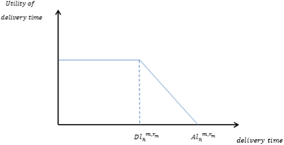
• Acce`ptable time window for hospitals is soft and utility of delivery time for blood m with age
$ {r}_m $
at hospitals in terms of desirable and acceptable late delivery time is generally illustrated in figure 2. -
• The initial inventory of the facilities is zero.

Utility of delivery time for blood m with age
 $ {r}_m $
at hospital h.

Notations
Table 2 represents the notations applied in the formulation of the proposed model.
Notations of the model

 $$ Min\hskip0.3em {Z}_1=\mathrm{Total}\ \mathrm{costs} $$
$$ Min\ ( Max)\hskip0.3em {Z}_2=\sum_o\sum_t\sum_m{W}_{ot}\left({ QB F}_{ot m}+{QB}_{ot m}\right)\;\sum_b\frac{dtra_{bo t}\;{ddr}_{bo}}{rr_{bo t}\;U\left({dpc}_{bo}\right)} $$
 $$ {\displaystyle \begin{array}{ll} Max\hskip0.42em {Z}_3& \hskip-0.7em ={\sum \limits}_{b\in K}{\sum \limits}_o{\sum \limits}_t{\sum \limits}_{e\in {V}^{\prime }}{\sum \limits}_m{\sum \limits}_{r_m=0}^1(\frac{U_m-{r}_m}{U_m})\frac{(1-{\lambda^{(3)}}_{bote}^{m,{r}_m})QM{A}_{bote}^{m,{r}_m}+(1-{\lambda^{(1)}}_{bote}^{m,{r}_m})Q{M}_{bote}^{m,{r}_m}}{d{f}_{otm}}U(t{d}_{bo}^{m,{r}_m})\\ {}& \hskip0.8em +{\sum \limits}_{b\in K}{\sum \limits}_o{\sum \limits}_t{\sum \limits}_{e\in {V}^{\prime }}{\sum \limits}_m{\sum \limits}_{r_m=2}(\frac{U_m-{r}_m+2}{U_m})\frac{(1-{\lambda^{(3)}}_{bote}^{m,{r}_m})QM{A}_{bote}^{m,{r}_m}+(1-{\lambda^{(1)}}_{bote}^{m,{r}_m})Q{M}_{bote}^{m,{r}_m}}{d_{otm}}U(t{d}_{bo}^{m,{r}_m})\\ {}& \hskip0.8em +{\sum \limits}_{b\in {K}^{\prime }}{\sum \limits}_o{\sum \limits}_t{\sum \limits}_{e\in {V}^{\prime }}{\sum \limits}_{r_1=0}^1(\frac{U_1-{r}_1}{U_1})\frac{(1-{\lambda^{(3)}}_{bote}^{m,{r}_m})QW{B}_{bote}^{r_1}}{d{f}_{ot1}}U(t{d}_{bo}^{1,{r}_1})\\ {}& \hskip0.8em +{\sum \limits}_{b\in {K}^{\prime }}{\sum \limits}_o{\sum \limits}_t{\sum \limits}_{e\in {V}^{\prime }}{\sum \limits}_{r_1=2}(\frac{U_1-{r}_1+2}{U_1})\frac{(1-{\lambda^{(3)}}_{bote}^{m,{r}_m})QW{B}_{bote}^{r_1}}{d_{ot1}}U(t{d}_{bo}^{1,{r}_1})\\ {}& \hskip0.8em +{\sum \limits}_{n\in I}{\sum \limits}_g{\sum \limits}_tp{l}_gus{f}_{gt}u{a}_grbc{c}_{gt}u{d}_{ng}{\varpi}_{ngt}^{(1)}\\ {}& \hskip0.8em +{\sum \limits}_{n\in {I}^{\prime },{I}^{{\prime\prime} }}{\sum \limits}_b{\sum \limits}_tpl{e}_bus{f}_{bt}^{\prime }ua{d}_brb{c}_{bt}ud{p}_{nb}{\varpi}_{nbt}^{(2)}\end{array}} $$
Subject to:
 $$ {\sum}_{rm}{QW}_{gbte}^{m,{r}_m}\le {capv}_e\hskip3.32em \forall m=1,g,b,t,e\in V $$
 $$ {\sum}_m{\sum}_{rm}\left({QM}_{bote}^{m,{r}_m}+{ QM A}_{bote}^{m,{r}_m}\right)\le {capv}_e\forall b\in K,o,t,e\in V^{\prime } $$
 $$ {\sum}_{rm}{QWB}_{bote}^{m,{r}_m}\le {capv}_e\hskip3.72em \forall m=1,b\in K^{\prime },o,t,e\in V^{\prime } $$
 $$ {\sum}_m{\sum}_{rm}{QMH}_{o_1{o}_2 te}^{m,{r}_m}\le {capv}_e\hskip1.44em \forall o\in H,t,e\in V^{{\prime\prime} } $$
 $$ {QD^{(1)}}_{ngt}={\varpi^{(1)}}_{ngt}\hskip3.32em \forall n\in I,g,t $$
 $$ {QD^{(2)}}_{nbt}={\varpi^{(2)}}_{nbt}\hskip3.32em \forall n\in {I}^{\prime },b,t $$
 $$ {QMAP}_{nbt m}={\varpi^{(2)}}_{nbt}\hskip3.96em \forall n\in {I}^{\prime \prime },b\in K,t,m $$
 $$ {QW}_{gbte}^{m,{r}_m}\le M\;{\psi^{(1)}}_{gbte}\hskip3.08em \forall m=1,g,b,t,e\in v,{r}_m $$
 $$ {\sum}_m{\sum}_{rm}\left({QM^{(1)}}_{khtv\prime}^{m,{r}_m}\hskip-0.14em +\hskip-0.14em {{QM A}^{(1)}}_{khtv\prime}^{m,{r}_m}\right)\le M{\psi^{(2)}}_{bote}\forall b\in k,o,t,e\in V^{\prime } $$
 $$ {QWB}_{bote}^{r_m}\le M\hskip0.2em {\psi^{(2)}}_{bote}\hskip3.84em \forall b\in k^{\prime },o,t,e,m=1,{r}_m $$
 $$ {QMH}_{o_1{o}_2t}^{m,{r}_m}\le M\;{\psi^{(3)}}_{o_1{o}_2 te}\hskip3.36em \forall {o}_1,{o}_2,t,e,m,{r}_m $$
 $$ {\varpi^{(1)}}_{ngt}\le \left[{rbcc}_{gt}+\left(1- mar\right)\right]\hskip3.2em \forall n,g,t $$
 $$ {\varpi^{(2)}}_{nbt}\le \left[{rbc}_{bt}+\left(1- mar\right)\right]\hskip3.68em \forall n\in I^{\prime },b\in K,t $$
 $$ {Y^{(2)}}_{bt}\le \left[{rbc}_{bt}+\left(1- mar\right)\right]\hskip3.44em \forall b\in k^{\prime },t $$
 $$ {\varpi^{(1)}}_{ngt}\le {Y^{(1)}}_{gt}\hskip3.84em \forall n\in I,\hskip0.36em g\in {J}^{\prime },t $$
 $$ {\varpi^{(2)}}_{nbt}\le {Y^{(2)}}_{bt}\hskip3.84em \forall n\in {I}^{\prime },b\in {K}^{\prime },t $$
 $$ {\varpi^{(2)}}_{nbt}\le \left[{rbc}_{bt}+\left(1- mar\right)\right]\hskip3.84em \forall n\in {I}^{\prime \prime },b\in K,t $$
 $$ {Y^{(1)}}_{gt}\le \left[{rbcc}_{gt}+\left(1- mar\right)\right]\hskip3.32em \forall g\in {J}^{\prime },t $$
 $$ {\psi^{(1)}}_{gb t e}\le \left[\frac{r_{gb t}\;U\left({dp}_{gb}\right)}{dd_{gb}{dtr}_{gb t}}+\left(1- avr\right)\right]\forall g\in J,b\in K,t,e\in V $$
 $$ {\psi^{(1)}}_{gb t e}\le \left[\frac{r_{gkt}\;U\left({dp}_{gb}\right)}{dd_{gb}\;{dtr}_{gb t}}+\left(1- avr\right)\right]\;{Y^{(2)}}_{bt}\forall g\in J,b\in {K}^{\prime },t,e\in V $$
 $$ {\psi^{(1)}}_{gb t e}\le \left[\frac{r_{gb t}\;U\left({dt}_{gb}\right)}{dd_{gb}\;{ dt r}_{gb t}}+\left(1- avr\right)\right]{Y^{(2)}}_{gt}\forall g\in {J}^{\prime },b\in k,t,e\in V $$
 $$ {\psi^{(1)}}_{gb t e}\le \left[\frac{r_{gb t}\;U\left({dt}_{gb}\right)}{dd_{gb}\;{ dt r}_{gb t}}+\left(1- avr\right)\right]{Y^{(1)}}_{gt}{Y^{(2)}}_{bt}\hskip1.6em \forall g\in {J}^{\prime },b\in {k}^{\prime },t,e\in v $$
 $$ {\psi^{(2)}}_{bo t e}\le \left[\frac{rr_{bo t}U\left({dpc}_{bo}\right)}{dtra_{bo t}{ddr}_{bo}}+\left(1- avr\right)\right]\hskip3.32em \forall b\in K,o\in H,t,e\in V^{\prime } $$
 $$ {\psi^{(2)}}_{bo t e}\le \left[\frac{rr_{bo t}U\left({dpc}_{bo}\right)}{dtra_{bo t}{ddr}_{bo}}+\left(1- avr\right)\right]\;{Y^{(3)}}_{ot}\hskip0.36em \forall b\in K,o\in H^{\prime },t,e\in V^{\prime } $$
 $$ {\psi^{(2)}}_{bo t e}\le \left[\frac{rr_{bo t}U\left({dpc}_{bo}\right)}{dtra_{bo t}{ddr}_{bo}}+\left(1\hskip-0.2em -\hskip-0.2em avr\right)\right]\;{Y^{(2)}}_{bt}\hskip0.48em \forall b\in K^{\prime },o\in H,t,e\in V^{\prime } $$
 $$ {\displaystyle \begin{array}{c}{\psi^{(2)}}_{bo t e}\le \left[\frac{rr_{bo t}U\left({dpc}_{bo}\right)}{dtra_{bo t}{ddr}_{bo}}+\left(1- avr\right)\right]\hskip0.24em {Y^{(2)}}_{bt}{Y^{(3)}}_{ot}\\ {}\hskip-8.72em \forall b\in K^{\prime },o\in H^{\prime },t,e\in V^{\prime}\end{array}} $$
 $$ {\sum}_{g\in J\prime }{Y^{(1)}}_{gt}\ge 1\hskip3.2em \forall t $$
 $$ {\sum}_{b\in K\prime }{Y^{(2)}}_{bt}\ge 1\hskip3.08em \forall t $$
 $$ {\sum}_{o\in H\prime }{Y^{(3)}}_{Ot}\ge 1\hskip3.08em \forall t $$
 $$ {\sum}_{g\in J}{\varpi^{(1)}}_{ngt}+{\sum}_{g\in {J}^{\prime }}{\varpi^{(1)}}_{ngt}=1\hskip3.44em \forall n\in I,t $$
 $$ {\sum}_b{\varpi^{(2)}}_{nbt}\hskip0.36em =1\hskip3.44em \forall n\in {i}^{\prime },t $$
 $$ {\sum}_{b\in K}{\varpi^{(2)}}_{nbt}\hskip0.36em =1\hskip3.44em \forall n\in {I}^{\prime \prime },t $$
 $$ {\sum}_{e\in V}{\psi^{(1)}}_{gbte}\le 1\hskip3.32em \forall g,b,t $$
 $$ {\sum}_{e\in V\prime }{\psi^{(2)}}_{bote}\le 1\hskip3.08em \forall b,o,t $$
 $$ {\sum}_b{\sum}_{e\in v}{\psi^{(1)}}_{gbte}\ge 1\hskip3.08em \forall g,t $$
 $$ {\sum}_o{\sum}_{e\in v\prime }{\psi^{(2)}}_{bote}\ge 1\hskip3.08em \forall b,t $$
 $$ {\sum}_g{\sum}_{e\in v}{\psi^{(1)}}_{gbte}\ge 1\hskip3.96em \forall b,t $$
 $$ {\sum}_{b\in K}{\sum}_{e\in V\prime }{\psi^{(2)}}_{bote}\ge 1\hskip3.96em \forall o,t $$
 $$ {\sum}_g{\sum}_b{\psi^{(1)}}_{gbte}=1\hskip3.84em \forall e\in v,t $$
 $$ {\sum}_b{\sum}_o{\psi^{(2)}}_{bote}=1\hskip3.6em \forall e\in {v}^{\prime },t $$
 $$ {\sum}_{o_1\in {H}_1}{\sum}_{e\in v{\prime\prime} }{\psi^{(3)}}_{{\mathrm{o}}_1{o}_2 te}\le 1\hskip3.08em \forall {o}_1\in {H}_1,t $$
 $$ {\sum}_{o_1\in {H}_1}{\sum}_{o_2\in {H}_2}{\psi^{(3)}}_{{\mathrm{o}}_1{o}_2 te}\le 1\hskip3.08em \forall e\in V^{{\prime\prime} },t $$
 $$ {\sum}_{o_2\in {H}_2}{\sum}_{e\in v{\prime\prime} }{\psi^{(3)}}_{{\mathrm{o}}_1{o}_2 te}\le 1\hskip3.08em \forall {o}_2\in {H}_2,t $$
 $$ {yl}_{bote}\le {\psi^{(2)}}_{bote}\hskip3.6em \forall b,o,t,e\in {v}^{\prime } $$
 $$ {\displaystyle \begin{array}{c}{\eta^{(1)}}_{bt}\;{\alpha^{(2)}}_{bt}\;{\sum}_{g\in J}{\sum}_{e\in V}\left(1-{\beta}_{bt m{r}_m}\right){QW}_{gbte}^{m,{r}_m}\\ {}\hskip-3.6em ={QMS_{bt}}^{m,{r}_1}\hskip3.6em \forall b,t,{r}_m\ge {r}_1\end{array}} $$
 $$ {\eta^{(3)}}_{bt}\;{\alpha^{(3)}}_{bt}\;{\sum}_{n\in i\prime }{QD^{(2)}}_{nbt}={QMS_{kt}}^{m,0}\hskip2.48em \forall b\in K,t,{r}_m\ge {r}_1 $$
 $$ {\sum}_{n\in I}{QD^{(1)}}_{ngt}+{I}_{g\left(t-1\right)}\le {cap}_g\hskip3.08em \forall g,t $$
 $$ {\displaystyle \begin{array}{c}{\sum}_{n\in I\prime }{QD^{(2)}}_{nbt}+{\sum}_g{\sum}_{e\in V}{\sum}_{r_1}\left(1-{\beta}_{bt{ mr}_m}\right)\\ {}\hskip-3.96em {QW}_{gbte}^{m,{r}_m}\le {capwb}_k\hskip3.96em \forall b,t\end{array}} $$
 $$ {\displaystyle \begin{array}{l}{\sum}_{b\in K}{\sum}_{e\in V\prime }{\sum}_{r_m=0}^1\\ {}\left[\left(\hskip-0.32em 1\hskip-0.3em -{\lambda^{(3)}}_{bote}^{m,{r}_m}\right){QM A}_{bote}^{m,{r}_m}\hskip-0.3em +\hskip-0.3em {IF A}_{o\left(t-1\right)m}\hskip-0.3em +\hskip-0.3em \left(\hskip-0.3em 1\hskip-0.3em -{\lambda^{(1)}}_{bote}^{m,{r}_m}\hskip-0.3em \right){QM}_{bote}^{m,{r}_m}\hskip-0.3em +\hskip-0.2em {IF}_{o\left(t-1\right)m}\right]\\ {}+{\sum}_{b\in K}{\sum}_{e\in V\prime }{\sum}_{r_{m=2}}\\ {}\left[\left(1-{\lambda^{(1)}}_{bote}^{m,{r}_m}\right){QM}_{bote}^{m,{r}_m}+\hskip-0.1em {I}_{o\left(t-1\right)m}\hskip-0.1em +\hskip-0.3em \left(\hskip-0.3em 1\hskip-0.3em -{\lambda^{(3)}}_{bote}^{m,{r}_m}\right){QM A}_{bote}^{m,{r}_m}\hskip-0.3em +\hskip-0.3em {IA}_{o\left(t-1\right)m}\right]\;\\ {}\le {capnw}_{om}\hskip3.36em \forall o,t,m\ge 2\end{array}} $$
 $$ {\displaystyle \begin{array}{l}{\sum}_{b\in K}{\sum}_{e\in V\prime }{\sum}_{r_1=0}^1\left(1-{\lambda^{(1)}}_{bote}^{m,{r}_m}\right){QM}_{bote}^{m,{r}_m}\\ {}\hskip2em +{\sum}_{b\in k\prime }{\sum}_{e\in v\prime }{\sum}_{r_M=0}^1\left(1-{\lambda^{(3)}}_{bote}^{m,{r}_m}\right){QWB}_{bote}^{m,{r}_m}+{IF}_{o\left(t-1\right)m}\\ {}\hskip2em +{\sum}_k{\sum}_{v\prime }{\sum}_{r_1=2}\left(1-{\lambda^{(1)}}_{bote}^{m,{r}_m}\right){QM}_{bote}^{m,{r}_m}\\ {}\hskip2em +{\sum}_{k\prime }{\sum}_{v\prime }{\sum}_{r_1=2}\left(1-{\lambda^{(3)}}_{bote}^{m,{r}_m}\right){QWB}_{bote}^{m,{r}_m}+{I}_{o\left(t-1\right)m}\\ {}\hskip2em \le {capnw}_{h1}\hskip3.96em \forall o,t,m=1\end{array}} $$
 $$ {\displaystyle \begin{array}{c}{I}_{gt}=\left(1-{\alpha^{(1)}}_{gt}\right)\;\left({\sum}_{n\in I}{QD^{(1)}}_{ngt}+{I}_{g\left(t-1\right)}\right)\\ {}\hskip4em -{\sum}_{b\in K}{\sum}_{r_1}{\sum}_{e\in V}{QW}_{gbte}^{m,{r}_m}\;\Big]\hskip3.32em \forall g,t\end{array}} $$
 $$ {\displaystyle \begin{array}{c}{I_{bt}}^{m,{r}_m}=\left(1-{\mu^{(1)}}_{b,t,m,{r}_m}\right)\left[{\mu^{(5)}}_{b,t,m,{r}_m}{{ QM S}_{bt}}^{m,{r}_1}+{I_{b\left(t-1\right)}}^{m,{r}_m}\right]\\ {}\hskip7em -{\sum}_o{\sum}_{e\in V\prime }{QM}_{bote}^{m,{r}_m}\hskip2.36em \forall b\in K,t,m=2,\dots, MP,{r}_m\end{array}} $$
 $$ {\displaystyle \begin{array}{c}{IA_{bt}}^{m,{r}_m}\hskip-0.1em =\hskip-0.14em \left(\hskip-0.3em 1\hskip-0.3em -\hskip-0.1em {\mu^{(2)}}_{b,t,m,{r}_m}\hskip-0.25em \right)\hskip-0.3em \left[{\mu^{(6)}}_{b,t,m,{r}_m}\hskip-0.1em {\sum}_{n\in I{\prime\prime}}\hskip-0.5em {{ QMA P}_{nbt}}^{m,{r}_m}\hskip-0.1em +\hskip-0.1em {IA_{b\left(t-1\right)}}^{m,{r}_m}\right]\\ {}\hskip3em -\left({\sum}_o{\sum}_{e\in V\prime }{QMA}_{bote}^{m,{r}_m}\right)\hskip1.08em \forall b\in K,t,m=2,\dots, MP,{r}_m\end{array}} $$
 $$ {\displaystyle \begin{array}{cc}{I}_{bt}^{m,{r}_m}& \hskip-1em =(1-{\beta}_{btm{r}_m})[{\eta}_{bt}^{(2)}[{\eta}_{bt}^{(2)}(1-{\alpha}_{bt}^{(2)}){\sum \limits}_g{\sum \limits}_{e\in V}(1-{\delta}_{gbte}^{(1)}1,{r}_1)\hskip2em Q{W}_{gbte}^{m,{r}_m}+{\eta}_{bt}^{(3)}{\eta}_{bt}^{(4)}(1-{\alpha}_{bt}^{(3)}){\sum \limits}_{n\in {I}^{\prime }}Q{D}_{nbt}^{(2)}+{I}_{b(t-1)}^{1,{r}_m}]\operatorname{}\\ {}& \hskip1em \operatorname{}\hskip-4em -{\sum \limits}_o{\sum \limits}_{e\in {V}^{\prime }}Q{M}_{bote}^{m,{r}_m}]\hskip3.5em \mathrm{\forall}b,t,m=1,{r}_1\end{array}} $$
 $$ {\displaystyle \begin{array}{ll}\hskip-2em I{F}_{O_1tm}& \hskip-1em ={\sum \limits}_{r_m=0}^1[(1-{\mu^{(4)}}_{o_1,t,m,{r}_m})[{\sum \limits}_{b\in K}{\sum \limits}_{e\in {V}^{\prime }}(1-{\lambda^{(1)}}_{bote}^{m,{r}_m})\hskip-0.8em Q{M}_{b{o}_1te}^{m,{r}_m}+I{F}_{o_1(t-1)m}]]\hskip-0.1em -{\sum \limits}_c{\sum \limits}_{r_m=0}^1\Big[\frac{1}{a}{\varphi^{(1)}}_{otc}^{1,{r}_1}\hskip6em CM{F}_{o_1tcm}^{(1)}[(1-{\mu^{(4)}}_{o_1,t,m,{r}_m})[{\sum \limits}_{b\in K}{\sum \limits}_{e\in {V}^{\prime }}(1-{\lambda^{(1)}}_{b{o}_1te}^{m,{r}_m})\hskip-1em Q{M}_{b{o}_1te}^{m,{r}_m}\operatorname{}\operatorname{}\operatorname{}\hskip4.4em \operatorname{}\operatorname{}\operatorname{}\hskip-4em +I{F}_{o_1(t-1)m}]]\Big]a+{\sum \limits}_{o_1\in {H}_2}{\sum \limits}_{e\in {V}^{{\prime\prime} }}\hskip3em {\sum \limits}_{r_m=0}^1QM{H}_{o_2{o}_1te}^{m,{r}_m}{\sum \limits}_c{\sum \limits}_{r_m=0}^1\Big[\frac{1}{a}\Big({\varphi^{(2)}}_{o_1tc}^{m,{r}_m}cm{f}_{o_1tcm}\hskip6.8em {\sum \limits}_{e\in {V}^{{\prime\prime} }}{\sum \limits}_{o_2\in {H}_2}(1-{\lambda^{(2)}}_{o_1{o}_2te}^{m,{r}_m})QM{H}_{o_2{o}_1te}^{m,{r}_m}\operatorname{}\operatorname{}\\ {}& \hskip0.50em +\Big({\sum \limits}_c{\sum \limits}_{r_m=0}^1({\varphi^{(1)}}_{o_1tc}^{m,{r}_m}cm{f}_{o_1tcm}\left(1-{\varphi^{(1)}}_{o_1tc}^{m,{r}_m}\right)\hskip6.7em ({\sum \limits}_{b\in K}{\sum \limits}_{e\in {V}^{\prime }}(1-{\lambda^{(1)}}_{b{o}_1te}^{m,{r}_m})Q{M}_{b{o}_1te}^{m,{r}_m}+I{F}_{o_1(t-1)m})\operatorname{}\operatorname{}\\ {}& \hskip-7em -\operatorname{}\operatorname{}\operatorname{}\Big[\frac{1}{a}{\varphi^{(1)}}_{o_1tc}^{m,{r}_m}cm{f}_{o_1tcm}(1-{\mu^{(4)}}_{o_1,t,m,{r}_m})\hskip-4.8em ({\sum \limits}_{b\in K}{\sum \limits}_{e\in {V}^{\prime }}\left(1-{\lambda^{(1)}}_{b{h}_1te}^{m,{r}_m}\right)Q{M}_{b{o}_1te}^{m,{r}_m}\hskip1em +I{F}_{o_1(t-1)m})]a\left)\right)\Big]a\hskip0em -{\sum \limits}_{o_2\in {H}_2}{\sum \limits}_{e\in {v}^{{\prime\prime} }}{\sum \limits}_{r_m=0}^1\hskip7em QM{H}_{o_1{o}_2te}^{m,{r}_m}\hskip3em \mathrm{\forall}{o}_1,t,m\ge 2\end{array}} $$
 $$ {\displaystyle \begin{array}{ll}IF{A}_{otm}& \hskip-13em ={\sum \limits}_c{\sum \limits}_{r_m=0}^1(1-{\mu^{(6)}}_{b,t,m,{r}_m})ca{f}_{otcm}[\left(1-{\mu^{(3)}}_{o,t,m,{r}_m}\right)\operatorname{}\\ {}& \operatorname{}\hskip-11em \left[{\sum \limits}_{b\in K}{\sum \limits}_{e\in {V}^{\prime }}(1-{\lambda^{(3)}}_{bote}^{m,{r}_m})QM{A}_{b{o}_1te}^{m,{r}_m}+IF{A}_{o(t-1)m}\right]]\\ {}\hskip6.2em \mathrm{\forall}o\in H,t,m\ge 2\end{array}} $$
 $$ {\displaystyle \begin{array}{cc}\hskip-6em I{F}_{o_1tm}& \hskip-2em ={\sum \limits}_c{\sum \limits}_{r_m=0}^1(1-{\varphi^{(1)}}_{otc}^{1,{r}_1})cm{f}_{o_1tcm}\left(1-{\mu^{(4)}}_{o_1,t,m,{r}_m}\right)\hskip-6.9em \Big[{\sum \limits}_{b\in K}{\sum \limits}_{e\in {V}^{\prime }}(1-{\lambda^{(1)}}_{bote}^{m,{r}_m})Q{M}_{b{o}_1te}^{m,{r}_m}\operatorname{}\\ {}& \hskip3.5em \operatorname{}+{\sum \limits}_{b\in {K}^{\prime }}\hskip-0.2em {\sum \limits}_{e\in {V}^{\prime }}(\hskip-0.2em 1\hskip-0.2em -\hskip-0.2em {\lambda^{(3)}}_{bote}^{m,{r}_m})QW{b^{(1)}}_{b{o}_1te}^{r_m}\hskip-0.2em +\hskip-0.2em I{F}_{o_1(t-1)m}\Big]\\ {}& \hskip-19.5em +{\sum \limits}_{e\in {V}^{{\prime\prime} }}{\sum \limits}_{O_2\in {H}_2}\hskip-3.3em {\sum \limits}_{r_m=0}^1(1-{\varphi^{(2)}}_{otc}^{m,{r}_m})cm{f}_{o_1tcm}(1-{\lambda^{(2)}}_{o_1{o}_2te}^{m,{r}_m})\hskip-11.2em QM{H}_{o_2{o}_1te}^{m,{r}_m}\\ {}& -{\sum \limits}_{e\in {V}^{{\prime\prime} }}{\sum \limits}_{o_2\in {H}_2}\hskip-6.5em {\sum \limits}_{r_m=0}^1Q{M^{(3)}}_{o_1{o}_2te}^{m,{r}_m}\hskip1em \mathrm{\forall}m=1,{o}_1\in {H}_1,t\end{array}} $$
 $$ {\displaystyle \begin{array}{cc}\hskip-32.5em {I}_{o_1tm}& \hskip-15.8em ={\sum \limits}_{r_m=2}[(1-{\mu^{(4)}}_{o_1,t,m,{r}_m})[{\sum \limits}_{b\in K}\hskip-7.3em {\sum \limits}_{e\in {V}^{\prime }}(1-{\lambda^{(1)}}_{bote}^{m,{r}_m})Q{M}_{b{o}_1te}^{m,{r}_m}+{I}_{o_1(t-1)m}]]\\ {}& \hskip-2.50em -{\sum \limits}_c{\sum \limits}_{r_m=2}\Big[\frac{1}{a}{\varphi^{(1)}}_{o_1tc}^{m,{r}_m}c{m}_{o_1tcm}(1-{\mu^{(4)}}_{o_1,t,m,{r}_m})\hskip0.5em ({\sum \limits}_{b\in K}{\sum \limits}_{e\in {V}^{\prime }}(1-{\lambda^{(1)}}_{b{o}_1te}^{m,{r}_m})Q{M}_{b{o}_1te}^{m,{r}_m}+{I}_{o_1(t-1)m})]a\operatorname{}\\ {}& \hskip-8.6em +{\sum \limits}_{o_2\in {H}_2}{\sum \limits}_{e\in {V}^{{\prime\prime} }}{\sum \limits}_{r_m=2}QM{H}_{o_2{o}_1te}^{m,{r}_m}\hskip-5em -{\sum \limits}_c{\sum \limits}_{r_m=2}\Big[\frac{1}{a}\Big({\varphi^{(2)}}_{o_1tc}^{m,{r}_m}cm{f}_{o_1tcm}{\sum \limits}_{e\in {V}^{{\prime\prime} }}\hskip-11em {\sum \limits}_{o_2\in {H}_2}(1-{\lambda^{(2)}}_{o_1{o}_2te}^{m,{r}_m})QM{H}_{o_2{o}_1te}^{m,{r}_m}\operatorname{}\operatorname{}\\ {}& \hskip-2em +\left({\sum \limits}_c{\sum \limits}_{r_m=0}^1({\varphi^{(1)}}_{o_1tc}^{m,{r}_m}cm{f}_{o_1tcm}\right(1-{\mu}_{o_1,t,m,{r}_m}^{(4)}\Big)\hskip4em \left({\sum \limits}_{b\in K}{\sum \limits}_{e\in {V}^{\prime }}(1-{\lambda^{(1)}}_{b{o}_1te}^{m,{r}_m})Q{M}_{b{o}_1te}^{m,{r}_m}+I{F}_{o_1(t-1)m}\right)\operatorname{}\\ {}& \hskip-8em \operatorname{}\operatorname{}\hskip1em -\Big[\frac{1}{a}{\varphi^{(1)}}_{o_1tc}^{m,{r}_m}cm{f}_{o_1tcm}(1-{\mu^{(4)}}_{o_1,t,m,{r}_m})\hskip6em ({\sum \limits}_{b\in K}{\sum \limits}_{e\in {V}^{\prime }}\hskip-0.2em (\hskip-0.2em 1\hskip-0.2em -\hskip-0.2em {\lambda^{(1)}}_{b{o}_1te}^{m,{r}_m})Q{M}_{b{o}_1te}^{m,{r}_m}\hskip-0.2em +\hskip-0.2em {I}_{o_1(t-1)m})\hskip-0.2em ]\hskip-0.2em a\Big)\hskip-0.2em )\hskip-0.2em )\hskip-0.2em ]a\\ {}& \hskip6.00em -{\sum \limits}_{o_2\in {H}_2}{\sum \limits}_{e\in {v}^{{\prime\prime} }}{\sum \limits}_{r_m=2}QM{H}_{o_2{o}_1te}^{m,{r}_m}\hskip1em \mathrm{\forall}{o}_1\in {H}_1,t,m\ge 2\end{array}} $$
 $$ {\displaystyle \begin{array}{cc}I{A}_{otm}& \hskip-4em ={\sum \limits}_c{\sum \limits}_{r_m=2}(1-{\varphi^{(1)}}_{otc}^{m,{r}_m})c{a}_{otcm}[(1-{\mu^{(3)}}_{o,t,m,{r}_m})\operatorname{}\\ {}& \operatorname{}\hskip1em [{\sum \limits}_{b\in K}{\sum \limits}_{e\in {V}^{\prime }}(1-{\lambda^{(3)}}_{bote}^{m,{r}_m})QM{A}_{bote}^{m,{r}_m}+I{A}_{o(t-1)m}]]\\ {}\hskip-21em \mathrm{\forall}o,t,m\ge 2\end{array}} $$
 $$ {\displaystyle \begin{array}{cc}\hskip-8.5em {I}_{o_1tm}& \hskip-3.8em ={\sum \limits}_c{\sum \limits}_{r_m=2}(1-{\varphi^{(1)}}_{o_1tc}^{m,{r}_m})cm{f}_{o_1tcm}\left(1-{\mu^{(4)}}_{o,t,,{r}_m}\right)\hskip-0.6em \Big[{\sum \limits}_{b\in K}{\sum \limits}_{e\in {V}^{\prime }}(1-{\lambda^{(1)}}_{b{o}_1te}^{m,{r}_m})Q{M}_{b{o}_1te}^{m,{r}_m}\operatorname{}\\ {}& \operatorname{}\hskip1em +{\sum \limits}_{b\in {K}^{\prime }}\hskip3.5em {\sum \limits}_{e\in {V}^{\prime }}(1-{\delta^{(2)}}_{b{o}_1te}^{m,{r}_m})QW{B}_{b{o}_1te}^{r_m}+I{F}_{o_1(t-1)m}]\\ {}& +{\sum \limits}_{e\in {V}^{{\prime\prime} }}\hskip1em {\sum \limits}_{o_2\in {H}_2}{\sum \limits}_{r_1=2}(1-{\varphi^{(2)}}_{o_1tc}^{m,{r}_m})cm{f}_{o_1tcm}(1-{\lambda^{(2)}}_{o_1{o}_2te}^{m,{r}_m})\hskip-0.2em QM{H}_{o_2{o}_1te}^{m,{r}_m}\\ {}& -{\sum \limits}_{e\in {V}^{{\prime\prime} }}{\sum \limits}_{o_2\in {H}_2}{\sum \limits}_{r_m=2}QM{H}_{o_2{o}_1te}^{m,{r}_m}\hskip-21em \mathrm{\forall}m=1,{o}_1\in {H}_1,t\end{array}} $$
 $$ {\displaystyle \begin{array}{cc}I{F}_{otm}& \hskip-1em ={\sum \limits}_c{\sum \limits}_{r_1=0}^1(1-{\varphi^{(1)}}_{otc}^{m,{r}_m})cm{f}_{o_1tcm}[\left(1-{\mu^{(4)}}_{o,t,m,{r}_m}\right)\hskip4em \Big[{\sum \limits}_{b\in K}{\sum \limits}_{e\in {V}^{\prime }}(1-{\lambda^{(1)}}_{bote}^{m,{r}_m})Q{M}_{bote}^{m,{r}_m}\operatorname{}\operatorname{}\\ {}& \hskip1em \operatorname{}\operatorname{}+{\sum \limits}_{b\in {K}^{\prime }}\hskip0.51em {\sum \limits}_{e\in {V}^{\prime }}(1-{\delta^{(2)}}_{bote}^{m,{r}_m})QW{B}_{bote}^{m,{r}_m}+I{F}_{o(t-1)m}]]\hskip-17.5em \mathrm{\forall}m=1,o\in {H}^{\prime },t\end{array}} $$
 $$ {\displaystyle \begin{array}{cc}\hskip-30em {I}_{otm}& \hskip-14.7em ={\sum \limits}_{r_m=2}[\left(1-{\mu^{(4)}}_{o,t,m,{r}_m}\right)\Big[{\sum \limits}_{b\in K}\hskip-5.8em {\sum \limits}_{e\in {V}^{\prime }}(1-{\lambda^{(1)}}_{bote}^{m,{r}_m})Q{M^{(2)}}_{bote}^{m,{r}_m}+{I}_{o(t-1)m}]\operatorname{}\\ {}& \hskip-2.5em -[{\sum \limits}_c{\sum \limits}_{r_m=2}\left[\frac{1}{a}{P^{(2)}}_{otc}^{m,{r}_m}c{m}_{otcm}[(1-{\mu^{(4)}}_{o,t,m,{r}_m})\hskip0.5em [{\sum \limits}_{b\in K}{\sum \limits}_{e\in {V}^{\prime }}(1-{\lambda^{(1)}}_{bote}^{m,{r}_m})Q{M}_{bote}^{m,{r}_m}+{I}_{o(t-1)m}]]\right]a\hskip-22em \mathrm{\forall}o\in {H}^{\prime },t,m\ge 2\end{array}} $$
 $$ {\displaystyle \begin{array}{cc}{I}_{otm}& \hskip-1em ={\sum \limits}_C{\sum \limits}_{r_m=2}(1-{\varphi^{(1)}}_{otc}^{m,{r}_m})c{m}_{otc1}[\left(1-{\mu^{(4)}}_{o,t,m,{r}_m}\right)\hskip-3.4em \Big[{\sum \limits}_{b\in K}{\sum \limits}_{e\in {V}^{\prime }}(1-{\lambda^{(1)}}_{bote}^{m,{r}_m})Q{M}_{bote}^{m,{r}_m}\operatorname{}\operatorname{}\\ {}& \hskip4.8em \operatorname{}\operatorname{}\hskip1em +{\sum \limits}_{b\in {K}^{\prime }}{\sum \limits}_{e\in {V}^{\prime }}(1-{\delta^{(2)}}_{bote}^{1,{r}_1})QW{b}_{bote}^{r_m}+{I}_{o(t-1)m}]]\hskip-16.5em \mathrm{\forall}m=1,o\in {H}^{\prime },t\end{array}} $$
 $$ {\displaystyle \begin{array}{cc}& \hskip-1.2em {QBF}_{o_1tm}={df}_{o_1tm}{\textstyle \hbox{-}}[{\sum \limits}_c{\sum \limits}_{r_m=0}^1\hskip-0.2em \Big[\frac{1}{a}{\varphi^{(1)}}_{O_1tc}^{m,{r}_m}cm{f}_{o_1tcm}[(1\hskip-0.2em -\hskip-0.2em {\mu^{(4)}}_{o_1,t,m,{r}_m}\hskip-0.1em )\hskip5em [{\sum \limits}_{b\in K}\hskip-0.2em {\sum \limits}_{e\in {V}^{\prime }}(1\hskip-0.2em -\hskip-0.2em {\lambda^{(1)}}_{b{o}_1te}^{m,{r}_m})Q{M}_{b{o}_1te}^{m,{r}_m}\operatorname{}\operatorname{}\operatorname{}\operatorname{}\\ {}& \operatorname{}\operatorname{}+I{F}_{o_1(t-1)m}]]]a\hskip1em +{\sum \limits}_c{\sum \limits}_{r_m=0}^1{\varphi^{(3)}}_{O_1tc}^{m,{r}_m}ca{f}_{o_1tm}\left[\right(1-{\mu^{(3)}}_{O_1,t,m,{r}_m}\Big)\hskip6em \Big[{\sum \limits}_{b\in K}\hskip-0.2em {\sum \limits}_{e\in {V}^{\prime }}(1\hskip-0.2em -\hskip-0.2em {\lambda^{(3)}}_{bote}^{m,{r}_m})QM{A}_{b{o}_1te}^{m,{r}_m}+IF{A}_{o_1(t-1)m}]]\\ {}& \hskip-1em +{\sum \limits}_c{\sum \limits}_{r_m=0}^1\Big[\frac{1}{a}({\varphi^{(2)}}_{o_1tc}^{m,{r}_m}\times cm{f}_{o_1tcm}{\sum \limits}_{e\in {V}^{{\prime\prime} }}\hskip-7em {\sum \limits}_{o_2\in {H}_2}(1-{\lambda^{(2)}}_{o_1{o}_2te}^{m,{r}_m})QM{H}_{o_2{o}_1te}^{m,{r}_m}\operatorname{}\operatorname{}\\ {}& \hskip2.9em +\left({\sum \limits}_c{\sum \limits}_{r_m=0}^1({\varphi^{(1)}}_{o_1tc}^{m,{r}_m}cm{f}_{o_1tcm}\right(1-{\mu^{(4)}}_{o_1,t,m,{r}_m}\Big)\hskip4.5em ({\sum \limits}_{b\in K}{\sum \limits}_{e\in {V}^{\prime }}(1-{\lambda^{(1)}}_{b{o}_1te}^{m,{r}_m})Q{M}_{b{o}_1te}^{m,{r}_m}+I{F}_{o_1(t-1)m})\operatorname{}\\ {}& \hskip-5.5em \operatorname{}\operatorname{}\operatorname{}-\Big[\frac{1}{a}{\varphi^{(1)}}_{o_1tc}^{m,{r}_m}cm{f}_{o_1tcm}(1-{\mu^{(4)}}_{o_1,t,m,{r}_m})\hskip7em (\hskip-0.2em {\sum \limits}_{b\hskip-0.1em \in \hskip-0.1em K}\hskip-0.2em {\sum \limits}_{e\hskip-0.1em \in \hskip-0.1em {V}^{\prime }}(\hskip-0.2em 1\hskip-0.2em -\hskip-0.2em {\lambda^{(1)}}_{b{o}_1te}^{m,{r}_m})\hskip-0.1em Q{M}_{b{o}_1te}^{m,{r}_m}\hskip-0.3em +\hskip-0.2em I{F}_{o_1(t-1)m})\hskip-0.3em ]\hskip-0.2em a)\hskip-0.3em \Big)\hskip-0.3em )\hskip-0.3em ]\hskip-0.3em a]\hskip-21em \mathrm{\forall}{o}_1,t,m\ge 2\end{array}} $$
 $$ {\displaystyle \begin{array}{cc}& \hskip-2em QB{F}_{o_1tm}=d{f}_{o_1tm}-[{\sum \limits}_c{\sum \limits}_{r_1=0}^1{\varphi^{(1)}}_{o_1tc}^{m,{r}_m}cm{f}_{o_1tc1}\left(1-{\mu^{(4)}}_{o_1,t,m,{r}_m}\right)\operatorname{}\\ {}& \hskip-5em \left[{\sum \limits}_{b\in K}{\sum \limits}_{e\in {V}^{\prime }}(1-{\lambda^{(1)}}_{b{o}_1te}^{m,{r}_m})Q{M}_{b{o}_1te}^{m,{r}_m}\hskip6em +\hskip-0.2em {\sum \limits}_{b\in {K}^{\prime }}\hskip-0.2em {\sum \limits}_{e\in {V}^{\prime }}\right(\hskip-0.2em 1\hskip-0.2em -\hskip-0.2em {\delta^{(2)}}_{b{o}_1te}^{1,{r}_1}\hskip-0.2em \Big)QW{B}_{b{o}_1te}^{m,{r}_m}+I{F}_{o_1(t-1)1}]\\ {}& \operatorname{}\hskip7.2em +\hskip-0.2em {\sum \limits}_{e\in {V}^{{\prime\prime} }}\hskip-0.2em {\sum \limits}_{o_2\in {H}_2}\hskip-0.2em {\sum \limits}_{r_1=0}^1{\varphi^{(1)}}_{o_1tc}^{m,{r}_m}cm{f}_{o_1tcm}(\hskip-0.2em 1\hskip-0.2em -\hskip-0.2em {\lambda^{(2)}}_{o_1{o}_2te}^{m,{r}_m})\hskip-9.6em QM{H}_{o_2{o}_1te}^{m,{r}_m}]\hskip3em \mathrm{\forall}m=1,{o}_1,t\end{array}} $$
 $$ {\displaystyle \begin{array}{cc}& \hskip-2em Q{B}_{o_1tm}={d}_{o_1tm}-[{\sum \limits}_c{\sum \limits}_{r_m=2}\Big[\frac{1}{a}{\varphi^{(1)}}_{o_1tc}^{m,{r}_m}cm{f}_{o_1tcm}[(1-{\mu^{(4)}}_{o_1,t,m,{r}_m})\hskip4em [{\sum \limits}_{b\in K}{\sum \limits}_{e\in {V}^{\prime }}(1-{\lambda^{(1)}}_{b{o}_1te}^{m,{r}_m})Q{M}_{b{o}_1te}^{m,{r}_m}\operatorname{}\operatorname{}\operatorname{}\operatorname{}\\ {}& \operatorname{}\operatorname{}\hskip1em +{I}_{o_1(t-1)m}]]]a\hskip-0.7em +{\sum \limits}_c{\sum \limits}_{r_m=2}{\varphi^{(1)}}_{o_1tc}^{m,{r}_m}ca{f}_{o_1tm}\left[\right(1-{\mu^{(3)}}_{o_1,t,m,{r}_m}\Big)\hskip4.6em \Big[{\sum \limits}_{b\in K}{\sum \limits}_{e\in {V}^{\prime }}(1-{\lambda^{(3)}}_{b{o}_1te}^{m,{r}_m})QM{A}_{b{o}_1te}^{m,{r}_m}+I{A}_{o_1(t-1)m}]]\\ {}& \hskip-3em +{\sum \limits}_c{\sum \limits}_{r_m=2}\Big[\frac{1}{a}\Big({\varphi^{(1)}}_{o_1tc}^{m,{r}_m}cm{f}_{o_1tcm}{\sum \limits}_{e\in {V}^{{\prime\prime} }}\hskip-8.6em {\sum \limits}_{o_2\in {H}_2}(1-{\lambda^{(2)}}_{o_1{o}_2te}^{m,{r}_m})QM{H}_{o_2{o}_1te}^{m,{r}_m}\operatorname{}\operatorname{}\\ {}& \hskip1em +\left({\sum \limits}_c{\sum \limits}_{r_m=0}^1{\varphi^{(1)}}_{o_1tc}^{m,{r}_m}cm{f}_{o_1tcm}\right(1-{\mu^{(4)}}_{o_1,t,m,{r}_m}\Big)\hskip2.5em ({\sum \limits}_{b\in K}{\sum \limits}_{e\in {V}^{\prime }}(1-{\lambda^{(1)}}_{b{o}_1te}^{m,{r}_m})Q{M}_{b{o}_1te}^{m,{r}_m}+{I}_{o_1(t-1)m})\operatorname{}\\ {}& \hskip-7.5em \operatorname{}\operatorname{}\operatorname{}\hskip1em -\Big[\frac{1}{a}{\varphi^{(1)}}_{o_1tc}^{m,{r}_m}cm{f}_{o_1tcm}(1-{\mu^{(4)}}_{o_1,t,m,{r}_m})\hskip7em (\hskip-0.2em {\sum \limits}_{b\in K}\hskip-0.2em {\sum \limits}_{e\in {V}^{\prime }}(\hskip-0.2em 1\hskip-0.2em -\hskip-0.2em {\lambda^{(1)}}_{b{o}_1te}^{m,{r}_m})Q{M}_{b{o}_1te}^{m,{r}_m}\hskip-0.2em +\hskip-0.2em {I}_{o_1(t-1)m})]a)\hskip-0.2em )\hskip-0.3em )\hskip-0.2em ]a]\hskip-21.5em \mathrm{\forall}{o}_1,t,m\ge 2\end{array}} $$
 $$ {\displaystyle \begin{array}{cc}& \hskip-3em Q{B}_{o_1tm}={d}_{o_1tm}-[{\sum \limits}_C{\sum \limits}_{r_m=2}{\varphi^{(1)}}_{o_1tc}^{m,{r}_m}cm{f}_{o_1tcm}\left(1-{\mu^{(4)}}_{o_1,t,m,{r}_m}\right)\operatorname{}\\ {}& \hskip-7.5em \operatorname{}\Big[{\sum \limits}_{b\in K}{\sum \limits}_{e\in {V}^{\prime }}(1-{\lambda^{(1)}}_{b{o}_1te}^{m,{r}_m})Q{M}_{b{o}_1te}^{m,{r}_m}\hskip3em +{\sum \limits}_{b\in {K}^{\prime }}{\sum \limits}_{e\in {V}^{\prime }}(1-{\delta^{(2)}}_{bote}^{m,{r}_m})QW{B}_{b{o}_1te}^{m,{r}_m}+{I}_{o_1(t-1)m}]\operatorname{}\\ {}& \hskip5.7em \operatorname{}+{\sum \limits}_{e\in {V}^{\prime }}{\sum \limits}_{o_2\in {H}_2}{\sum \limits}_{r_m=2}{\varphi^{(1)}}_{otc}^{m,{r}_m}cm{f}_{o_1tcm}(1-{\lambda^{(2)}}_{o_1{o}_2te}^{m,{r}_m})\hskip-12.5em QM{H}_{o_2{o}_1te}^{m,{r}_m}]\hskip3em \mathrm{\forall}m=1,{o}_1,t\end{array}} $$
 $$ {I}_{g0}\hskip-0.2em =\hskip-0.1em {I_{k0}}^{m,{r}_m}\hskip-0.1em =\hskip-0.1em {IA_{k0}}^{m,{r}_m}\hskip-0.1em =\hskip-0.1em {I_{k\prime 0}}^{r_1}={I_{k\prime 0}}^{r_1}\hskip-0.1em =\hskip-0.1em {IF}_{o0m}\hskip-0.1em =\hskip-0.1em {IF a}_{o0m}\hskip-0.1em =\hskip-0.1em {I}_{o0m}\hskip-0.1em =\hskip-0.1em {Ia}_{o0m}\hskip-0.1em =\hskip-0.1em 0 $$
 $$ {QMA^{(2)}}_{bote}^{m,{r}_m}=0\hskip3.96em \forall m=1,b\in K,o\in {H}^{\prime },t,e\in {V}^{\prime },{r}_m $$
 $$ {\displaystyle \begin{array}{cc}& \hskip-5em {\sum \limits}_{r_m=0}^1QM{H}_{o_1{o}_2te}^{m,{r}_m}= Min\Big\{({\sum \limits}_{r_m=0}^1[(1-{\mu^{(4)}}_{o,t,m,{r}_m})[{\sum \limits}_{b\in K}\hskip-4.5em {\sum \limits}_{e\in {V}^{\prime }}(1-{\lambda^{(1)}}_{b{o}_1te}^{m,{r}_m})Q{M}_{b{o}_1te}^{m,{r}_m}\\ {}& \hskip1em +I{F}_{o_1(t-1)m}]]\hskip0.2em -{\sum \limits}_c{\sum \limits}_{r_m=0}^1[\frac{1}{a}{\varphi^{(1)}}_{otc}^{m,{r}_m}cm{f}_{o_1tcm}[\left(1-{\mu^{(4)}}_{o_1,t,m,{r}_m}\right)\\ {}& \hskip2.5em [{\sum \limits}_{b\in K}{\sum \limits}_{e\in {V}^{\prime }}(1-{\lambda^{(1)}}_{b{o}_1te}^{m,{r}_m})Q{M}_{b{o}_1te}^{m,{r}_m}+I{F}_{o_1(t-1)m}]]]a\\ {}& \hskip-2em -({\sum \limits}_c{\sum \limits}_{r_m=0}^1{\varphi^{(1)}}_{o_1tc}^{m,{r}_m}cm{f}_{o_1tcm}\left(1-{\mu^{(4)}}_{o_1,t,m,{r}_m}\right)\hskip1em ({\sum \limits}_{b\in K}{\sum \limits}_{e\in {V}^{\prime }}(1-{\lambda^{(1)}}_{b{o}_1te}^{m,{r}_m})Q{M}_{b{o}_1te}^{m,{r}_m}\\ {}& \hskip1em +I{F}_{o_1(t-1)m})\hskip-5em -[\frac{1}{a}{\varphi^{(1)}}_{o_1tc}^{m,{r}_m}cm{f}_{o_1tcm}(1-{\mu^{(4)}}_{o_1,t,m,{r}_m})({\sum \limits}_{b\in K}{\sum \limits}_{e\in {V}^{\prime }}\left(1-{\lambda^{(1)}}_{b{o}_1te}^{m,{r}_m}\right)Q{M}_{b{o}_1te}^{m,{r}_m}\\ {}& \hskip1em +I{F}_{o_1(t-1)m})]a))),\hskip4em (d{f}_{o_2tm}-[{\sum \limits}_c{\sum \limits}_{r_m=0}^1[\frac{1}{a}{\varphi^{(1)}}_{o_2tc}^{m,{r}_m}cm{f}_{o_2tcm}[(1-{\mu^{(4)}}_{o_1,t,m,{r}_m})\\ {}& \hskip-3em [{\sum \limits}_k{\sum \limits}_{v^{\prime }}(1-{\lambda^{(1)}}_{b{o}_1te}^{m,{r}_m})Q{M}_{b{o}_2te}^{m,{r}_m}+I{F}_{o_2(t-1)m}]]]a\hskip-3em +{\sum \limits}_c{\sum \limits}_{r_m=0}^1{\varphi^{(3)}}_{o_2tc}^{m,{r}_m}ca{f}_{o_1tcm}\\ {}& \hskip1em [\left(1-{\mu^{(3)}}_{o_1,t,m,{r}_m}\right)\hskip3.00em [{\sum \limits}_{b\in K}{\sum \limits}_{e\in {V}^{\prime }}\left(1-{\lambda^{(3)}}_{bote}^{m,{r}_m}\right)QM{A}_{b{o}_2te}^{m,{r}_m}+IF{A}_{o_2(t-1)m}]]\\ {}& \hskip-3em +({\sum \limits}_c{\sum \limits}_{r_m=0}^1{\varphi^{(1)}}_{o_2tc}^{m,{r}_m}cm{f}_{o_2tcm}\left(1-{\mu^{(4)}}_{o_2,t,m,{r}_m}\right)({\sum \limits}_{b\in K}{\sum \limits}_{e\in {V}^{\prime }}(1-{\lambda^{(1)}}_{b{o}_2te}^{m,{r}_m})Q{M}_{b{o}_2te}^{m,{r}_m}\\ {}& \hskip1em +I{F}_{o_2(t-1)m})\hskip-6em -[\frac{1}{a}{\varphi^{(1)}}_{o_2tc}^{m,{r}_m}cm{f}_{o_2tcm}(1-{\mu^{(4)}}_{o_2,t,m,{r}_m})({\sum \limits}_{b\in K}\hskip4.5em {\sum \limits}_{e\in {V}^{\prime }}(1-{\lambda^{(1)}}_{b{o}_2te}^{m,{r}_m})Q{M}_{b{o}_2te}^{m,{r}_m}\\ {}& \hskip1em +I{F}_{o_2(t-1)m})]a))])\}{\psi}_{o_1{o}_2te}^{(3)}\hskip-20em \mathrm{\forall}{o}_1,{o}_2,t,e,m\ge 2,{r}_m\end{array}} $$
 $$ {\displaystyle \begin{array}{cc}& \hskip-9em {\sum \limits}_{r_m=2}QM{H}_{o_1{o}_2te}^{m,{r}_m}= Min\{({\sum \limits}_{r_m=2}[(1-{\mu^{(4)}}_{o_1,t,m,{r}_m})\hskip-2em [{\sum \limits}_{b\in K}{\sum \limits}_{e\in {V}^{\prime }}(1-{\lambda^{(1)}}_{b{o}_1te}^{m,{r}_m})Q{M}_{b{o}_1te}^{m,{r}_m}\\ {}& +{I}_{o_1(t-1)m}]\hskip-2.5em -{\sum \limits}_c{\sum \limits}_{r_m=2}[\frac{1}{a}{\varphi^{(1)}}_{o_1tc}^{m,{r}_m}c{m}_{o_1tcm}[\left(1-{\mu^{(4)}}_{o_1,t,m,{r}_m}\right)\\ {}& \hskip1.5em [{\sum \limits}_{b\in K}{\sum \limits}_{e\in {V}^{\prime }}(1-{\lambda^{(1)}}_{b{o}_1te}^{m,{r}_m})Q{M}_{b{o}_1te}^{m,{r}_m}+{I}_{o_1(t-1)m}]]]a]\\ {}& \hskip2.3em -({\sum \limits}_c{\sum \limits}_{r_m=2}{\varphi^{(1)}}_{o_1tc}^{m,{r}_m}cm{f}_{o_1tcm}\left(1-{\mu^{(4)}}_{o_1,t,m,{r}_m}\right)({\sum \limits}_{b\in K}\hskip-6.3em {\sum \limits}_{e\in {V}^{\prime }}(1-{\lambda^{(1)}}_{b{o}_1te}^{m,{r}_m})Q{M}_{b{o}_1te}^{m,{r}_m}\\ {}& \hskip1em +{I}_{o_1(t-1)m})\hskip-5em -[\frac{1}{a}{\varphi^{(1)}}_{o_1tc}^{m,{r}_m}cm{f}_{o_1tcm}(1-{\mu^{(4)}}_{o_1,t,m,{r}_m})({\sum \limits}_{b\in K}\hskip-1em {\sum \limits}_{e\in {V}^{\prime }}(1-{\lambda^{(1)}}_{b{o}_1te}^{m,{r}_m})Q{M}_{b{o}_1te}^{m,{r}_m}\\ {}& \hskip1em +{I}_{o_1(t-1)m})]a))),\hskip2.4em ({d}_{o_2tm}-[{\sum \limits}_c{\sum \limits}_{r_m=2}[\frac{1}{a}{\varphi^{(1)}}_{o_2tc}^{m,{r}_m}c{m}_{o_2tcm}[(1-{\mu^{(4)}}_{o_2,t,m,{r}_m})\\ {}& \hskip0.4em [{\sum \limits}_{b\in K}{\sum \limits}_{e\in {V}^{\prime }}(1-{\lambda^{(1)}}_{b{o}_2te}^{m,{r}_m})Q{M}_{b{o}_2te}^{m,{r}_m}+{I}_{o_2(t-1)m}]]]a\\ {}& \hskip-5.5em +{\sum \limits}_c{\sum \limits}_{r_m=2}{\varphi^{(3)}}_{o_2tc}^{m,{r}_m}c{a}_{o_2tcm}[(1-{\mu^{(3)}}_{o_2,t,m,{r}_m})\hskip2em [{\sum \limits}_{b\in K}{\sum \limits}_{e\in {V}^{\prime }}(1-{\lambda^{(3)}}_{b{o}_2te}^{m,{r}_m})QM{A}_{b{o}_2te}^{m,{r}_m}\\ {}& \hskip1em +I{A}_{o_2(t-1)m}]]\hskip-2.5em +({\sum \limits}_c{\sum \limits}_{r_m=2}{\varphi^{(1)}}_{o_2tc}^{m,{r}_m}cm{f}_{o_2tcm}\left(1-{\mu^{(4)}}_{o_2,t,m,{r}_m}\right)\\ {}& \hskip-1em ({\sum \limits}_{b\in K}{\sum \limits}_{e\in {V}^{\prime }}(1-{\lambda^{(1)}}_{b{o}_2te}^{m,{r}_m})Q{M}_{b{o}_2te}^{m,{r}_m}+{I}_{o_2(t-1)m})\\ {}& \hskip-5em -[\frac{1}{a}{\varphi^{(1)}}_{o_2tc}^{m,{r}_m}cm{f}_{o_2tcm}(1-{\mu^{(4)}}_{o_2,t,m,{r}_m})({\sum \limits}_{b\in K}\hskip4em {\sum \limits}_{e\in {V}^{\prime }}(1-{\lambda^{(1)}}_{b{o}_2te}^{m,{r}_m})Q{M}_{b{o}_2te}^{m,{r}_m}\\ {}& \hskip1em +{I}_{o_2(t-1)m})]a)])\}{\psi}_{o_1{o}_2te}^{(3)}\hskip-15.5em \mathrm{\forall}{o}_1,{o}_2\in H,t,e\in {V}^{{\prime\prime} },m\ge 2\end{array}} $$
 $$ {\displaystyle \begin{array}{ll}& \hskip-2em {\sum \limits}_{r_m=0}^1QM{H}_{o_1{h}_2te}^{m,{r}_m}=\\ {}& \hskip1em Min\{{\sum \limits}_c{\sum \limits}_{r_m=0}^1(1-{\varphi}_{o_2tc}^{(1)m,{r}_m})cm{f}_{o_1tcm}\left(1-{\mu}_{o_1,t,m,{r}_m}^{(4)}\right)\\ {}& \hskip1em [{\sum \limits}_{b\in K}{\sum \limits}_{e\in {V}^{\prime }}(1-{\lambda^{(1)}}_{b{o}_1te}^{m,{r}_m})Q{M}_{b{o}_1te}^{m,{r}_m}\\ {}& \hskip1em +{\sum \limits}_{b\in {K}^{\prime }}{\sum \limits}_{e\in {V}^{\prime }}(1-{\lambda^{(3)}}_{b{o}_1te}^{m,{r}_m})QW{B}_{b{o}_2te}^{m,{r}_m}+I{F}_{o_1(t-1)m}],\\ {}& \hskip1em d{f}_{o_2tm}-[{\sum \limits}_c{\sum \limits}_{r_m=0}^1{\varphi^{(1)}}_{o_2tc}^{m,{r}_m}cm{f}_{o_2tcm}\left(1-{\mu^{(4)}}_{o_2,t,m,{r}_m}\right)\\ {}& \hskip1em [{\sum \limits}_{b\in K}{\sum \limits}_{e\in {V}^{\prime }}(1-{\lambda^{(1)}}_{b{o}_2te}^{m,{r}_m})Q{M}_{b{o}_2te}^{m,{r}_m}\\ {}& \hskip1em +{\sum \limits}_{b\in {K}^{\prime }}{\sum \limits}_{e\in {V}^{\prime }}(1-{\delta^{(2)}}_{b{o}_2te}^{m,{r}_m})QW{B}_{b{o}_2te}^{m,{r}_m}\\ {}& \hskip1em +I{F}_{o_2(t-1)m}]]\}{\psi}_{o_1{o}_2te}^{(3)}\hskip3em \mathrm{\forall}m=1,{o}_1,{o}_2\in H,t,e\in {V}^{{\prime\prime}}\end{array}} $$
 $$ {\displaystyle \begin{array}{cc}& \hskip-30em {\sum \limits}_{r_1=2}QM{H}_{o_1{o}_2te}^{m,{r}_m}=\hskip2em Min\{{\sum \limits}_C{\sum \limits}_{r_1=2}(1-{\varphi^{(1)}}_{o_1tc}^{m,{r}_m})cm{f}_{o_1tcm}[\left(1-{\mu^{(4)}}_{o_1,t,m,{r}_m}\right)\\ {}& \hskip-11em [{\sum \limits}_{b\in K}{\sum \limits}_{e\in {V}^{\prime }}(1-{\lambda^{(1)}}_{b{o}_1te}^{m,{r}_m})Q{M}_{b{o}_1te}^{m,{r}_m}\hskip0em +{\sum \limits}_{b\in {K}^{\prime }}{\sum \limits}_{e\in {V}^{\prime }}(1-{\delta^{(2)}}_{b{o}_1te}^{m,{r}_m})QW{B}_{b{o}_2te}^{m,{r}_m}\\ {}& +{I}_{o_1(t-1)m}]],\hskip-2.8em {d}_{o_2tm}-[{\sum \limits}_C{\sum \limits}_{r_1=2}{\varphi^{(1)}}_{o_2tc}^{m,{r}_m}c{m}_{o_2tcm}\\ {}& [(1-{\delta^{(2)}}_{b{o}_2te}^{m,{r}_m})\hskip-10.3em [{\sum \limits}_{b\in K}{\sum \limits}_{e\in {V}^{\prime }}(1-{\lambda^{(1)}}_{b{o}_2te}^{m,{r}_m})Q{M}_{b{o}_2te}^{m,{r}_m}\\ {}& \hskip-8.5em +{\sum \limits}_{b\in {K}^{\prime }}{\sum \limits}_{e\in {V}^{\prime }}(1-{\delta^{(2)}}_{b{o}_1te}^{m,{r}_m})QW{B}_{b{o}_2te}^{m,{r}_m}\\ {}& \hskip1.6em +{I}_{o_2(t-1)m}]]]\}{\psi}_{o_1{o}_2te}^{(3)}\hskip3em \mathrm{\forall}m=1,{o}_1,{o}_2\in H,t,e\in {V}^{{\prime\prime}}\end{array}} $$
 $$ {\displaystyle \begin{array}{ll}& \hskip-1em {Y^{(1)}}_{gt},{Y^{(2)}}_{bt},{Y^{(3)}}_{ot},{\varpi^{(1)}}_{ngt},{\varpi^{(2)}}_{nbt},{\psi^{(1)}}_{gbte},{\psi^{(2)}}_{bote},{\psi^{(3)}}_{o_1{o}_2te}\\ {}& \in \hskip-0.2em \{0,\hskip-0.2em 1\},{Q{D}^{(1)}}_{ngt},{Q{D}^{(2)}}_{nbt},{QW}_{gbte}^{m,{r}_m},{QWB}_{bote}^{m,{r}_m},{QM}_{bote}^{m,{r}_m},{QMA}_{bote}^{m,{r}_m},\\ {}& {QMH}_{o_1{o}_2te}^{m,{r}_m},\hskip-0.13em {QBF}_{\hskip-0.2em otm},\hskip-0.2em {QB}_{otm},\hskip-0.2em {QMS_{bt}}^{m,{r}_m}\hskip-0.2em ,\hskip-0.2em {QMA_{nbt}}^{m,{r}_m}\hskip-0.2em ,{I}_{gt},\hskip-0.1em {I_{bt}}^{m,{r}_m}\hskip-0.2em ,\hskip-0.1em {I{A}_{bt}}^{m,{r}_m},\\ {}& {IF}_{otm},{IFA}_{otm},{I}_{otm},{IA}_{otm}\epsilon {Z}^{+}\end{array}} $$
The first objective is associated with minimizing costs (see the “Appendix” section). The costs include, respectively, the following:
Cost of opening temporary facilities, transportation cost of blood products by various vehicles (including horizontal collaborations), production cost of blood products through separation and apheresis, processing cost at facilities, advertising cost, cost of improving staff safety and prevention, cost of cross-match test, returning cost, holding cost, cost of late delivery of blood products, waste cost, cost of inspection, and inspection error and shortage cost of fresh and non-fresh blood at hospitals.
The second objective minimizes maximum unsatisfied demands of hospitals with high priority and low route value.
The final objective function intends to maximize the quality of blood product delivered to hospitals and blood transfusion centers, and the satisfaction of donors. Quality of blood product delivery is based on of the blood freshness, utility of lead time of blood products, and rate of coverage of blood demand, and blood donors’ satisfaction is a function of staff performance, space and facilities, and the utility of distance and announcements. The constraints are described in Table 3.
Description of constraints of the proposed model

Interval Evidential Reasoning (IER) Approach
Since some parameters of the model, especially those derived from human judgment, are inevitably uncertain, there is an obvious need to apply methods handling uncertainty. This paper addresses this by employing Interval Evidential Reasoning (IER) approach, which is extension of the Evidential Reasoning (ER) approach under interval uncertainty.
The ER approach has been developed for multiple attribute decision analysis (MADA) problems based upon the Dempster–Shafer (D–S) theory of evidence and decision theory.Reference Dempster 31 –Reference Yang, Wang and Xu 35 It describes (model) various types of uncertainties such as vagueness, incompleteness, and ignorance using a belief structure. Experts express their opinions in belief structure, which includes well-organized grade and belief degree. Then, the D–S theory is used to aggregate the opinions. A complete explanation of the algorithm can be found in.Reference Yang, Wang and Xu 35
In many decision situations, an expert may be unable to represent judgment by giving a precise number and information will have been lost. In such conditions, using interval numbers can be a sensible option that is nearly in accord with uncertainty characteristics of human thought, and provides more flexibility for experts. Therefore, the IER approach has been applied in this study. There are 3 types of interval uncertainty that can be covered by the IER approach: interval grade, interval belief degree, and interval data.34,35 We address the first type of interval uncertainties, which allows the grade to be assigned to an individual or interval value. To simplify the understanding of this approach, we describe its procedure with an example.Reference Chin, Wang and Yang 36
Suppose that there are 5 experts with equal relative weight (0.2) to estimate a parameter in an IER belief structure using a set of 5 grades: G = {1, 2, 3, 4, 5}. Each grade in the whole range of G can be assigned to the parameter, and the possible grading matrix is defined as follows:
 $$ \mathrm{Possible}\ \mathrm{grading}\ \mathrm{matrix}=\left[\begin{array}{ccccc} 1& 1\hbox{-} 3& 1\hbox{-} 5& 1\hbox{-} 7& 1\hbox{-} 9\\ {}& 3& 3\hbox{-} 5& 3\hbox{-} 7& 3\hbox{-} 9\\ {}& & 5& 5\hbox{-} 7& 5\hbox{-} 9\\ {}& & & 7& 7\hbox{-} 9\end{array}\right] $$
Based on the above assumptions, some possible statements of the experts’ opinion on the parameter in the IER belief structure are as follows:
Statement 1: Vacillate between individual grades with different belief degrees. For example, an expert gives the parameter grade 1 with belief degree of 40%, and grade 2 with the belief degree of 60%: {(1, 40%), (2, 60%)}.
Statement 2: Vacillate between interval grades and interval grades with different belief degrees. For example, an expert estimates the parameter by giving grade [3-4] with belief degree of 30%, and grade 5 with the belief degree of 50%: {(3-4, 30%), (5, 50%)}.
Statement 3: Unawareness about the parameter. Because grading scale is [1-5], it will be modeled as: {(1-5, 100%)}.
It is important to note that when the total belief degree is less than 100%, as in Statement 2, the remaining percentage reflects a lack of information. This unassigned portion can be distributed across any point on the grading scale.
By calculating the expected values, For example, the belief structures in all statements can be modeled using expected values, as shown below:
 $$ {\displaystyle \begin{array}{l}\left\{\left( 1, 40\%\right),\left( 2, 60\%\right)\right\}\to 1\times 4 0\%+ 2\times 60\%= 1.6=\left[ 1. 6\hbox{-} 1. 6\right],\\ {}\left\{\left( 3\hbox{-} 4, 30\%\right),\left( 5, 50\%\right)\right\}\to \left[ 3\hbox{-} 4\right]\times 30\%+ 5\times 5 0\%+\left[ 1\hbox{-} 5\right]\times 20\%\\ {}=\left[ 3. 6\hbox{-} 4. 7\right],\left\{\left( 1\hbox{-} 5, 100\%\right)\right\}\to \left[ 1\hbox{-} 5\right]\times 1 00\%=\left[ 1\hbox{-} 5\right].\end{array}} $$
Finally, the experts’ opinions are integrated to decrease estimation error. The collective estimation of the parameter (E
 $ (S)\Big) $
is obtained from the weighted sum of the expected values of the 5 experts as follows:
 $$ E(S)={\sum}_{l=1}^5{\lambda}_lE\left({S}^l\right), $$
Where
 $ {\lambda}_l $
is the weight of expert
 $ l $
and
 $ E\left({S}^l\right) $
is expected value of expert
 $ l $
about the parameter.
Now, the problem is how the model with these interval parameters can be solved. The lower and upper boundaries of the parameters are considered as variables and value of them is computed through proposed algorithms.
Solution Method and Results
The presented model is an integer nonlinear programming model that is an NP-hard problem. Factors such as high number of constraints, existence of binary variables, and the multi-objective of the model made the model more complex. To solve such problems on a real scale, heuristic and meta-heuristic methods are used. In this study, we applied NSGAII and MOPSO meta-heuristic algorithms. NSGAII and MOPSO algorithms are the most widely used and most powerful meta-heuristic algorithms for solving multi-objective optimization problems that have been considered in the last 2 decades. Since implementing such complex problems on real scale (real life case) requires implementing a massive project (predicting the values of parameters) in disastrous situations (in the aftermath of an earthquake), 15 numerical examples are provided in small, medium, and large sizes to evaluate the efficiency of the algorithms and compare results. The value of the demand and the reliability of routes and facilities in each period are estimated in the form of IER data as described in section 4, and are converted to interval data. The other parameters of the examples are randomly generated based on the uniform distribution. Table 4 indicates the dimensions of the designed problems.
Dimensions of 15 designed problems

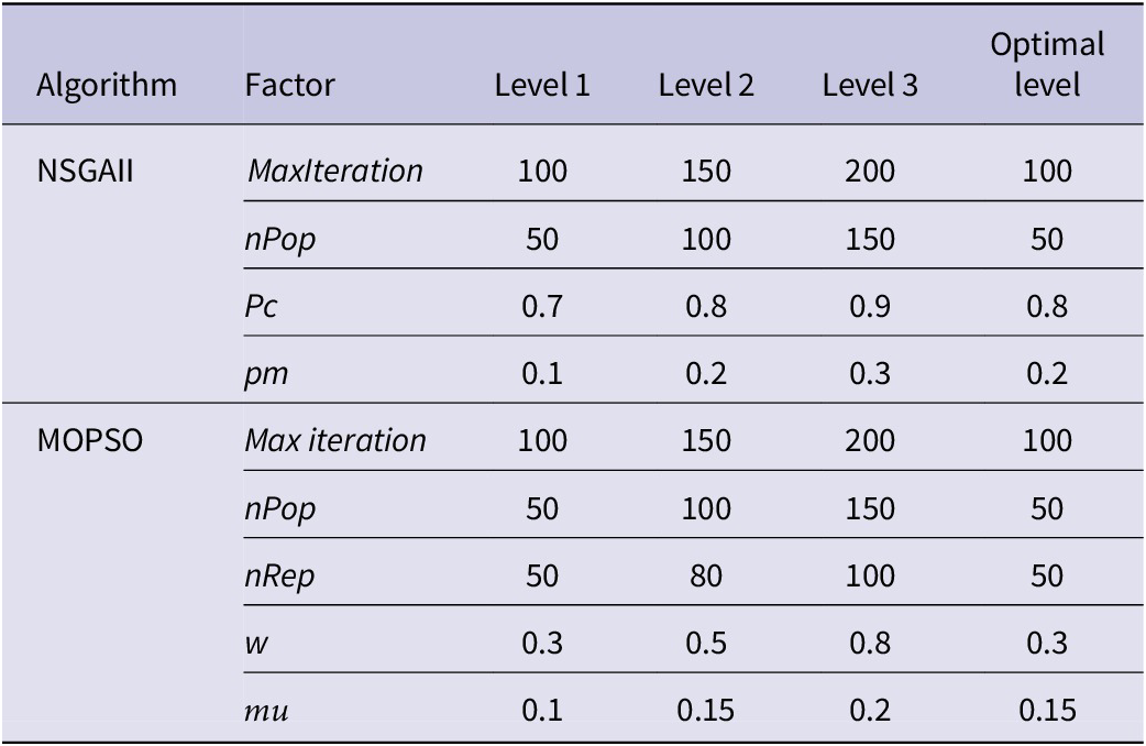
Since the output of meta-heuristic algorithms is strongly dependent on input parameters of algorithms, the Taguchi method is used to set parameters. In this method, appropriate factors are first identified and the levels of each of them are selected. Then, the appropriate experiment design for these factors is determined. After determining the design of the experiment, the experiments are carried out and analyzed to find the optimal combination of the parameters. In this study, according to Table 5, for each algorithm and factor, 3 levels are considered and the experiments have been designed and implemented.
Different defined levels and optimal level of parameters for proposed algorithms

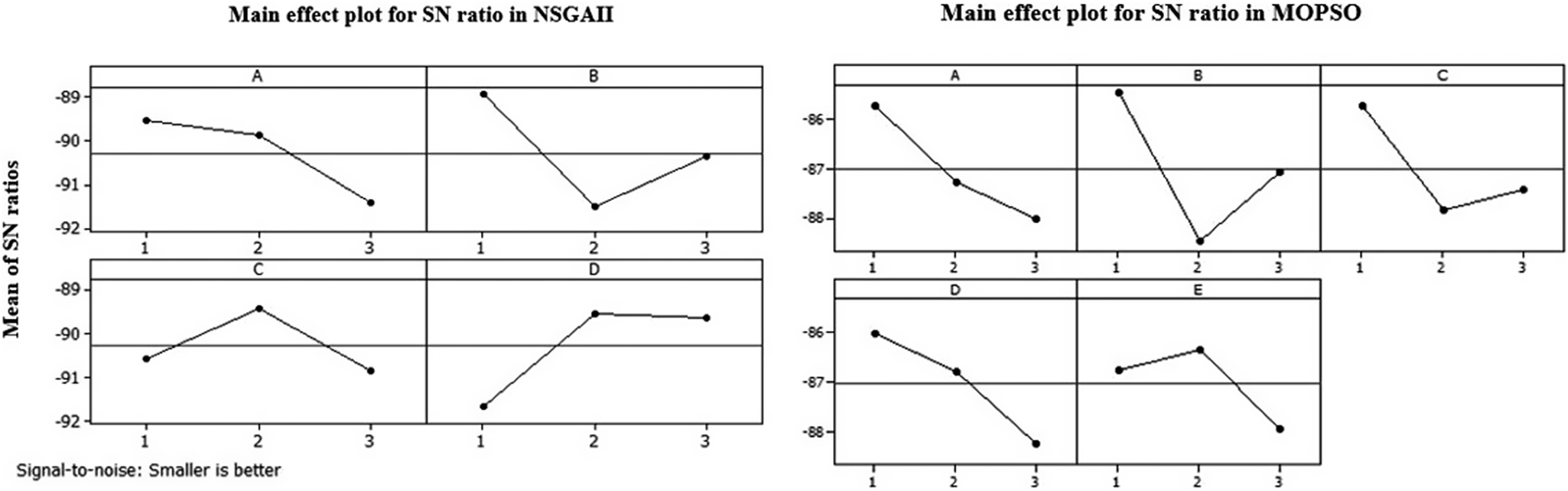
In the Taguchi method, the Signal/Noise (S/N) ratio is used for analysis, in which S refers to the response variable and N is standard deviation. Therefore, the higher ratio, the more favorable it is. The considered response variable is mean ideal distance (MID), and since it is “less and better,” the corresponding S/N ratio is calculated using equation (Reference Nagurney, Masoumi and Yu2).
 $$ S/N=-10\;\mathit{\log}\;\left(\;\frac{1}{n}{\sum}_{i=1}^n{y_i}^2\right) $$
Values of this ratio have been obtained for each algorithm shown in Figure 3.
Main effects plot for SN ratios in NSGAII and MOPSO algorithm.

Based on the results, the parameters are adjusted. The last column of Table 5 shows the final parameters of both algorithms.
In the following, the problems are solved through both algorithms. Figure 4 depicts the solved sample of the first problem.
Pareto solutions of problem 1 using MOPSO and NSGAII algorithm.

In order to compare the results obtained from the algorithms, the following comparative criteria are used:
-
• Number of Pareto Solution (NPS)
-
• Mean Ideal Distance (MID)
-
• Spacing (S)
-
• Maximum Diversity (MD)
-
• Time (T)
Computational results of these criteria for all problems have been shown in Table 6.
Table 6.Value of comparative criteria in both NSGAII and MOPSO algorithms for all designed problems

Figure 5 illustrates average values of the criteria for both of the algorithms in different sizes.
Average values of the criteria for MOPSO and NSGAII algorithms in different sizes.

According to figure 5:
-
• For medium and large problems, the value of the NPS criterion in the NSGAII algorithm is more, which causes more alternative solutions to decision-makers and supply chain managers.
-
• In MOPSO algorithm, the MID criterion in small and medium sizes has less value than solutions of the NSGAII algorithm. Therefore, the MOPOS algorithm is superior.
-
• Since the MOPOS algorithm has a lower S value in all 3 sizes, it is more favorable than the NSGAII algorithm.
-
• For medium and large problems, the fourth criterion (MD) of the MOPSO algorithm is more than NSGAII (with a small difference).
-
• The last criterion is time, and the results show that the MOPSO algorithm is more efficient in terms of this criterion.
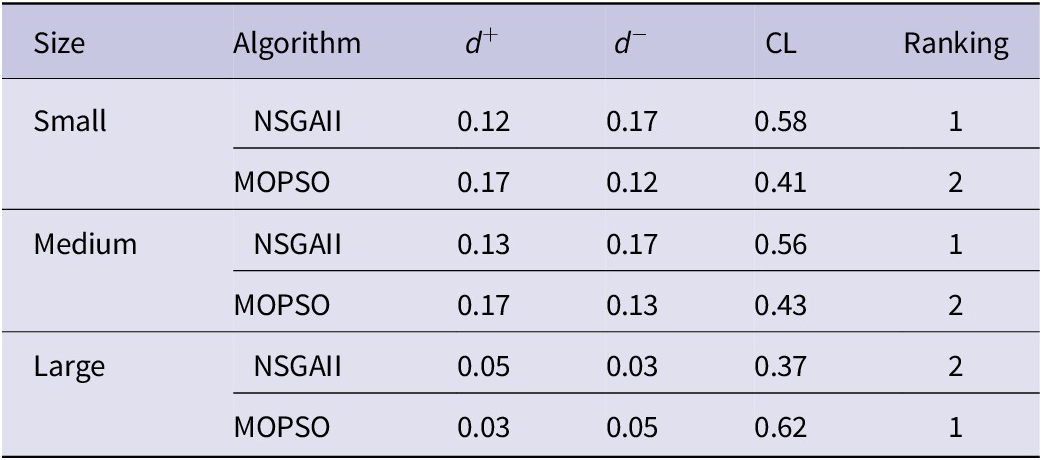
To determine the best algorithm of any size, the TOPSIS method is applied, the results of which are presented in Table 7. It should be noted that the weight of the criteria is considered the same.
Ranking of the algorithms in different sizes based on results of TOPSIS method

According to the results, the MOPSO algorithm in small size and the NSGAII algorithm in medium and large size have higher efficiency.
Finally, a sensitivity analysis has been conducted on some parameters including blood demand, reliability of routes, and transportation cost. The values of the parameters are changed by 20%, 50%, and 80% less and more than the base value, and the model was re-analyzed using the NSGAII and MOPSO algorithms. Table 8 indicates the changes of the objective functions against parameter changes using both algorithms.
Sensitivity analysis on different parameters using the NSGAII and MOPSO algorithms

Based on the results of Table 8, it can be concluded that when hospital demand for blood increases, blood shortage in hospitals, and accordingly shortage cost, increases due to the limited blood receiving capacity of blood centers and hospitals and limited number and capacity of vehicles. In addition, to meet the demand of patients, it may be necessary to establish more temporary blood collection and transfusion centers, which leads to higher costs. In this case, the cost of advertising to attract the donors, the cost of holding, inspection, evaluation, producing blood products, and therefore, the total cost, also increases. Because of the low demand coverage rate and the utility of lead time of blood products through vehicles with limited capacity, the quality of blood delivery is reduced. As shown in Table 8, with increase in transportation cost, the amount of blood products sent to centers and hospitals is reduced, causing an increase in unfulfilled demand and shortages, as well as total costs. By reducing the demand coverage rate, the quality of delivery and the value of the third objective function decreases as well. In the case of low route reliability, the amount of blood allocation and the utility of lead time is reduced. Consequently, the cost associated with shortages rises, while the quality of blood delivery diminishes.
Conclusion
Natural disasters, especially earthquakes, disrupt the blood supply chain, and designing an efficient and effective blood supply chain in such conditions is absolutely essential. For this purpose, we presented a LAVRTW model for 4-level and dynamic blood supply chains in emergency response to earthquakes that optimizes economical and humanitarian objectives. The model aims to determine the number and location of temporary facilities, allocation of donors to blood collection and blood transfusion centers, allocation of vehicles to each facility, amount of blood production, transfer and inventory in the relevant facilities, and optimal route of each facility. The main contributions of this paper are providing new criteria for location-allocation-vehicle routing decisions (blood supply chain design decisions) in disasters, formulating quality costs along with humanitarian objectives by defining “Route Value” and “Quality of Blood Delivery” concepts, incorporating satisfaction of all levels of the supply chain and staff, and considering the 4-level structure of the blood supply chain, various types of blood products with different lifetime derived from both separation and apheresis, reliability of routes and facilities, horizontal collaborations, and C/T ratio. Moreover, blood demand and reliability are assumed to be uncertain and the IER approach has been employed to handle the uncertainty. Due to the computational complexity of the proposed model, the NSGAII and MOPSO algorithms have been utilized for computing the solution of the model. These algorithms are implemented on 15 numerical examples in different sizes, and the obtained solutions are compared using the TOPSIS method based on criteria including NPS, MID, S, MD, and T. The findings suggest that while MOPSO is more appropriate for large-scale problems, NSGA-II demonstrates higher efficiency for small and medium-sized instances.
The following items are suggested for future studies:
-
• Incorporating compatibility of blood groups.
-
• Adding air vehicles, like helicopters, to existing vehicles.
-
• Using other meta-heuristic algorithms to solve the model and compare with the obtained results.
-
• Since the model has been formulated based on the realistic assumptions and complexities of one of the biggest blood transfusion centers in Iran to overcome its challenges, it has high compatibility to real-world situations and can be applied to real scale problems.
-
• Using other approaches like fuzzyReference Özceylan and Paksoy 37,38 and robustReference Babaee Tirkolaee, Goli and Pahlevan 39 Reference Khalilpourazari and Arshadi Khamseh ,40 to handle uncertainty.
Data availability statement
No external datasets were used or generated for this study.
Author contribution
Studying conceptions, reviewing literature, providing mathematical model, solving the numerical examples: Shiva Moslemi.
Providing the model, solution method, analysis and interpretation of results: Prof. Abolfazl Mirzazadeh and Dr Mohammadi.
Funding statement
This research received no specific grant from any funding agency in the public, commercial, or not-for-profit sectors.
Competing interests
The authors declare none.
Ethical standard
This research involved expert discussions with personnel at the Blood Transfusion Center of Tehran to understand the blood supply chain process. No personal or sensitive data were collected, and no ethical approval was required.
Appendix
In this section, the first objective function which aims to minimize total costs is presented as follows: