Nomenclature
- ATM
-
air traffic management
- TBO
-
trajectory-based operation
- ICAO
-
International Civil Aviation Organisations
- FRA
-
free route airspace
- Eurocontrol
-
European organisation for the safety of air navigation
- SESAR
-
single European sky ATM research
- FF
-
free flight
- RTCA
-
radio technical commission for aeronautics
- CAVs
-
connected and automated vehicles
- TCAS
-
traffic alert and collision avoidance system
- ACAS
-
airborne collision avoidance system
- CAAC
-
Civil Aviation Administration of China
- ADS-B
-
automatic dependent surveillance-broadcast
1.0 Introduction
As the demand for air transportation continues to grow, the service capacity of the traditional airspace management model is becoming a critical factor impeding the development of aviation. In the traditional management pattern, which centres on air traffic controllers as the primary decision-makers, airspace capacity is largely dependent on controller workload. However, as flight transport demands continue to rise, the tradition controller-centric air traffic control pattern is inevitably exacerbating manpower requirements and increasing workloads. Concurrently, airspace sectorisation is becoming more granular and the airway network structure more complex. This has multiplied the frequency of control handovers and coordination, placing increasing pressure on air traffic management (ATM). Therefore, transferring partial control responsibilities from the ground to the aircraft, enabling pilots to make autonomous, aircraft-centric decisions – known as the autonomous operation mode – is poised to be the key breakthrough in resolving this bottleneck.
While a precise domestic or international definition of autonomous operation in civil aviation has not yet been formed, a fundamental consensus on its core concept exists. This involves: transferring partial control responsibilities and authority to the airborne side, thereby granting pilots greater decision-making autonomy; developing airborne-centric operation situation awareness; and supplementing this with comprehensive ATM services from the ground, such as information, meteorology and surveillance [Reference Zhou, Zhang and Li1]. Reviewing the evolution of ATM, autonomous operation is not a standalone operational mode, but rather a product of continuous integration, iteration and innovation built upon the foundations of various advanced ATM concepts.
-
(1) The Decision Basis for Autonomous Operation: Trajectory-based Operation (TBO) [2]. The TBO concept was first proposed by the International Civil Aviation Organisation (ICAO) in its Global Air Traffic Management Operational Concept (ICAO Doc 9854). Its core idea is to use precise 4D trajectories (4DT) spanning the entire operational lifecycle of the aircraft to establish a shared understanding of the aircraft’s operation among multiple stakeholders, including ATC units, airlines and airports. Through collaborative decision-making, it aims to achieve fine-grained management of flight trajectories, ensuring the controllability and predictability of the entire flight operation, thereby elevating the level of precision and collaboration in ATM. The 4DT can accurately describe the aircraft’s spatial state information at any moment. Based on this information, media, aircraft and ATC units can better conduct flight management, thus significantly improving air traffic operational efficiency.
-
(2) The Airspace Environment for Autonomous Operation: Free Route Airspace (FRA) [Reference Kraus3]. To further break the ‘human-in-the-loop’ operational characteristic of tradition control, the European Organisation for the Safety of Air Navigation (Eurocontrol) launched the FRA concept, which is also an important component of the Single European Sky ATM Research (SESAR) project. Under this model, aircraft are no longer dependent on traditional fixed routes or ATC waypoints. Instead, pilots are permitted to autonomously select their flight paths within a specific airspace, thereby improving operational efficiency, saving time and reducing fuel costs. In 2024, Eurocontrol published its latest Free Route Airspace Implementation Plan, which schedules the transformation of traditional controlled airspace to FRA across Europe by 2030.
-
(3) The Ultimate Concept of Autonomous Operation: Free Flight (FF) [4]. Radio Technical Commission for Aeronautics (RTCA) first proposed the FF concept in 1995. The core of this concept is that aircraft can autonomously plan their flight paths from the departure airport to the destination airport, and freely choose flight state parameters such as heading, speed and altitude. Compared to traditional control models, FF grants pilots an extremely high degree of freedom in sensing, decision-making and planning. However, constrained by the technological standards and supporting infrastructure of the era, this operation concept was not widely implemented on a global scale.
The autonomous operation mode will drive the evolution of air traffic control (ATC) from a centralised pattern to a distributed one [Reference Pappas, Tomlin and Lygeros5]. Through real-time information exchange between the aircraft’s airborne systems and the ATC system, it enables shared situational awareness between pilots and controllers, permitting pilots to autonomously plan and adjust their routes based on real-time airspace information and flight requirements. Therefore, in this mode, the assessment of airspace operation situation will be dominated by the on-board system, and the object of assessment will be expanded from the original fixed air routes to any location point in the airspace. In the future development of autonomous operation mode, the number of aircraft and aircraft types in the airspace is expected to increase significantly, and the flexibility of air route selection will also be greatly improved, which brings convenience and efficiency to air transportation and, at the same time, greatly increases the operation risk. Meanwhile, the autonomous operation model imposes stricter requirements on the immediacy and dynamism of risk assessment, which not only need to be able to capture and respond to the immediate changes in the airspace but also require a high level of adaptability and dynamic adjustment capabilities. This demand becomes particularly challenging given the limitations of current computing performance. Therefore, there is an urgent need for an airspace risk assessment method under the autonomous operation mode of aircraft to improve the capability of airspace safety situation awareness in the future autonomous operation mode.
Airspace operation situation can be reflected by air traffic complexity, and the concept of air traffic complexity is introduced to assess the difficulty and effort required to manage air traffic safely. Since the air traffic situation is formed by the combined effects of airspace, traffic flow, controllers and environment, most domestic and international scholars’ studies on airspace operational situation are based on evaluating the perspective of air traffic complexity, which is conducted in terms of intrinsic properties and dynamic density of air traffic. The study of air traffic intrinsic properties considers that the complexity of air traffic situation is related to the overall airspace structure, the relationship between individual aircraft and the relationship between aircraft and key references in the surrounding environment, which focuses on portraying the intrinsic order of air traffic flow. Dynamic density aspect research is that air traffic complexity will be directly reflected through the controller’s workload, so density, dynamics, conflict traffic constitutive indexes and airspace constitutive indexes [Reference Zhang6] are established to describe the operation of the air traffic system, objectively reflecting the correlation between the air traffic situation and the controller’s workload. In terms of air traffic complexity assessment, Gianazza et al. [Reference Gianazza and Guittet7] obtained the correlation between air traffic complexity indicators through principal component analysis and further leveraged the neural network to mine the intrinsic connection between the indicators and the sector structure. Towards the needs of future next-generation ATM systems, Prandini [Reference Prandini, Piroddi and Puechmorel8] comprehensively analysed the existing air traffic complexity assessment and prediction methods, and discussed whether these methods can be transferred to autonomous ATM systems. Radanovic et al. [Reference Radanovic, Eroles and Koca9] introduced the ecosystem theory into the assessment of airspace complexity and analysed the spatial and temporal interdependence between aircraft by taking the domino effect into account to deduce the airspace complexity. Hu’s team [Reference Zhang, Hu and Zhang10, Reference Ye, Hu and Zhang11] proposed an airspace complexity model based on the proximity effects, probability factors and the degree of connectivity to characterise the change process of the airspace traffic situation, and constructed a distance factor and a conflict factor based on the structural elements of the air traffic to reflect the relative distances between the aircraft and the influence of the trajectory intersections on the airspace complexity, so as to realise the objective description of the airspace situation.
As the importance of airspace operation situation assessment in ensuring aviation safety continues to grow, current research is directly oriented towards the measurement of airspace operation situation. The primary task of air traffic management is to ensure the safe operation of air traffic and to prevent unsafe aviation incidents as much as possible. Therefore, many experts and scholars approach the measurement of airspace operation situation from the perspective of conflicts between aircraft, assessing the safety of the airspace to ensure the safe operation of aircraft. Alam et al. [Reference Alam, Lokan and Aldis12] proposed an evolutionary multi-objective scenario-based approach to systematically identify airspace collision risk thresholds under different control operations. Netjasov F developed conflict risk assessment models for three stages of airspace management: strategic planning [Reference Netjasov13], tactical planning [Reference Netjasov14] and current-day planning [Reference Netjasov and Babić15]. Zhang [Reference Zhang, Shortle and Sherry16] used the Monte Carlo algorithm to simulate the characteristics of the corridor concept and aircraft movement within the corridor, combined with dynamic event trees to assess the effectiveness of collision avoidance safety layers. Skorupski [Reference Skorupski17] calculated the probability of aircraft collision based on Petri net and incorporated computer expert knowledge in the form of fuzzy inference rules to assess the consequences of collisions. Ma et al. [Reference Ma, Cai and Alam18] calculated the distribution of collision risk within the airspace and used image processing techniques to classify risk patterns.
Focusing solely on specific conflict events will make airspace operation situation awareness lack a global perspective. In recent years, graph theory and complex network theory have been introduced into the study of the airspace operation situation, which not only endows the physical structure of the air traffic operation situation but also provides local and global network indicators, offering new research perspectives and methodologies for the airspace operation situation. Wang et al. [Reference Wang, Song and Wen19] established a two-layer multilevel dynamic network model, proposed an air traffic complexity vector based on complex network metrics and combined with a clustering algorithm to classify the airspace complexity model. Nguyen et al. [Reference Nguyen and Alam20] used an extended clustering model to identify potential collision clusters and calculated the collision risk of each cluster to achieve the risk assessment of the airspace. WEN et al. [Reference Lin, Wen and Wu21] introduced a three-dimensional (3D) velocity obstacle method to construct an airspace conflict network. Based on this conflict network, they designed a comprehensive robustness index to realise the robustness analysis of various types of networks [Reference Lin, Wen and Wu22], utilised complex network indexes based on aircraft clusters to classify busy and idle time periods in sectors [Reference Peng, Wen and Kong23] and combined conflict network topology indicators to form an optimal sample set for predicting airspace situation [Reference Wen, Peng and Bi24]. Zhang et al. [Reference Zhang, Lyu and Wan25] established an air traffic situation network based on the conflict relationship under the aircraft position deviation, and combined with the evolution analysis method to explore the evolution mechanism of an airspace safety situation.
In order to meet the new requirements for refined perception of an airspace safety situation under the autonomous operation mode, Brázdilová et al. [Reference Brázdilová, Cásek and Kubalčík26] constructed an air traffic complexity index and evaluated its potential application in the future distributed ATM system. Chen et al. [Reference Chen, Hu and Yang27], focusing on FRA, proposed a rapid trajectory planning method based on visibility graphs and Dijkstra’s algorithm, and a conflict-free trajectory generation method based on a continuous dynamics aircraft position updating model and local conflict detection and resolution algorithm. Wang et al. [Reference Wang and Guo28] proposed a real-time calculation method of air traffic complexity to reflect the complexity effects of aircraft position, speed and heading on each location point in the airspace. Peng et al. [Reference Peng, Wen and Wu29] proposed a refined flight conflict network construction model under the TBO operation mode by comprehensively considering the error factors such as communication and navigation surveillance. Targeting the refined requirements for aircraft conflict detection under autonomous operation mode, Zhang et al. [Reference Zhang, Wang and Yi30] proposed a flight conflict network model that comprehensively considers both positional proximity and the velocity obstacle relationship. In summary, existing research on airspace operation risk assessment mainly focuses on the traditional ATM model, with few studies emphasising future autonomous operation mode and evaluating airspace operation risk from the perspective of aircraft. Under the autonomous operation mode, the aircraft relies on its own perception, decision-making and control system to accomplish the flight task, and real-time risk measurement is the key to ensure the safety and reliability of autonomous operation. The existing studies can hardly meet the requirement of real-time risk measurement at any location in the airspace and cannot provide decision support for the subsequent aircraft air route planning and airspace resource allocation and utilisation.
In recent years, potential field theory has provided new perspectives for describing interactions between objects. Potential field theory converts the studied elements into potential field sources and characterises the interactions between the elements through virtual potential fields. The theory was first applied to robot path planning [Reference Latombe31] and has since been extended to the field of traffic flow by research scholars, achieving important research results. For example, Wang et al. [Reference Wang, Wu and Zheng32] proposed a driving safety field model based on potential field theory, calculating the virtual mass of various traffic elements to describe their impact on driving risk. Li et al. [Reference Li, Song and Cao33] improved the vehicle safety field by considering the risk effects from different directions, introducing the concept of an elliptical vehicle safety field. Li et al. [Reference Li, Gan and Zhou34] evaluated the driving risk during lane changing based on the safety potential field theory. Then, towards the scenario of mixed operation of manned and unmanned vehicles in ground traffic, a safety potential field model [Reference Li, Wang and Zhang35] for mixed traffic flow was proposed. Ma et al. [Reference Ma, Dong and Yin36] evaluated the multi-vehicle interaction risk of connected and automated vehicles (CAVs) in the weaving area based on the potential field theory. Ai et al. [Reference Ai, Li and Han37] introduced the concept of a multi-aircraft interaction risk potential field, establishing a potential risk field for interactions between aircraft and between aircraft and route points or routes. Currently, the application of potential field theory in traffic flow research is primarily focused on ground traffic. However, in the air traffic flow scenario, aircraft maintain safe distances from other aircraft and restricted areas while following predetermined routes. This operating mode suggests that elements in the airspace radiate an energy field and interact with each other through virtual forces. Therefore, in order to further improve the cognitive level of the airspace safety situation under autonomous operation mode and improve flight safety, this paper proposes a rapid risk assessment method for any location point in the airspace based on the theory of potential field toward the future autonomous operation mode, which provides technical support for the safe implementation of the future autonomous operation mode.
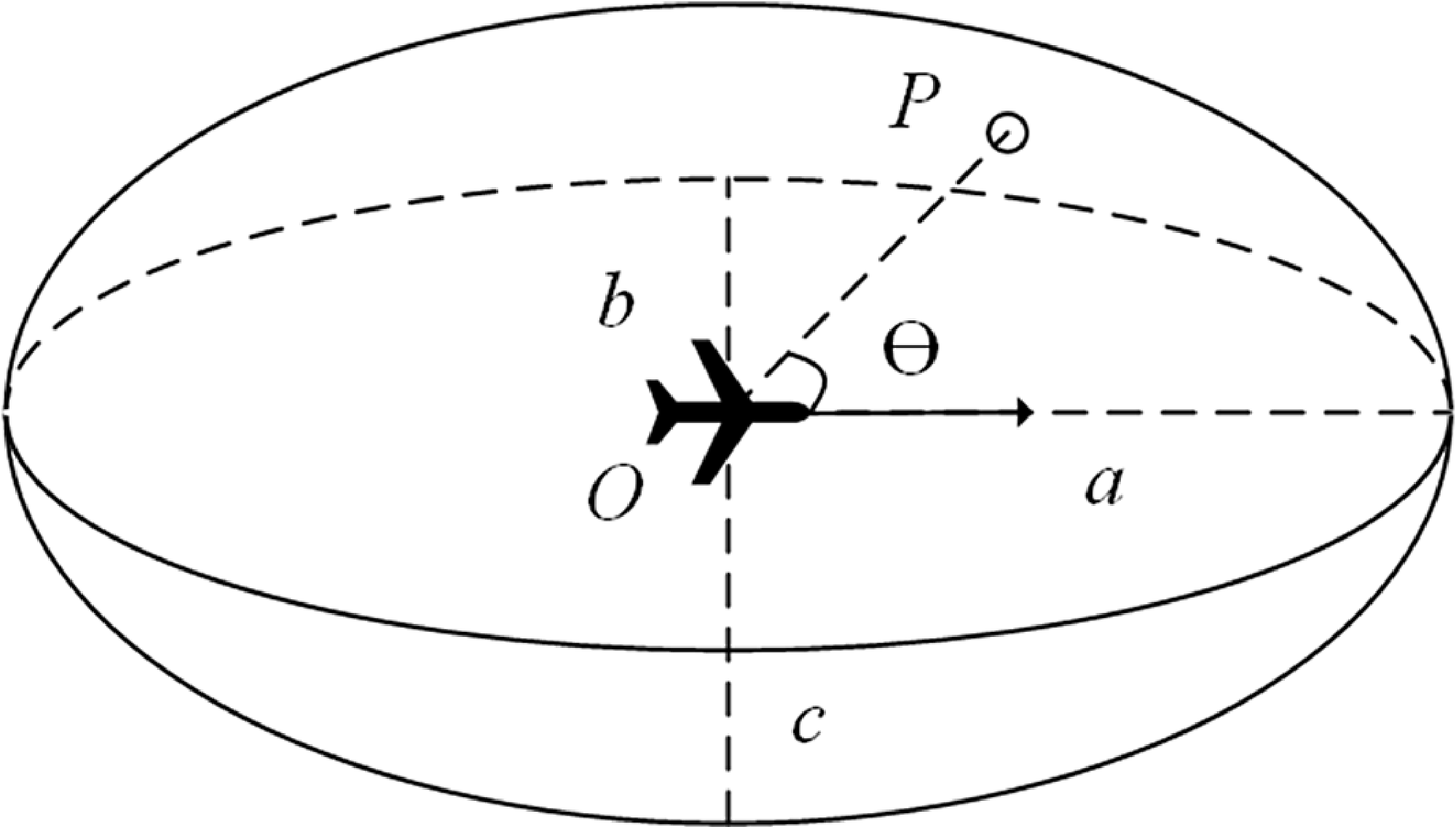
Aircraft ellipsoid risk zone.

2.0 Airspace risk modeling
The risk level at any arbitrary point within the airspace is determined by the superposition of risk influences exerted by multiple aircraft. Therefore, the key to airspace risk modeling lies in reasonably quantifying the risk influence mechanism of a single aircraft on the surrounding spatial points. Drawing on the concept of aircraft collision protection zones, the Reich model has laid the theoretical foundation for collision determination and collision risk assessment and has been widely applied in route separation safety assessments [Reference Zhang, Wang and Yi30, Reference Reich38]. In such studies, the aircraft protection zone is typically abstracted into geometric shapes such as cuboids, cylinders or ellipsoids. Inspired by this and considering that the influence of an aircraft does not propagate infinitely, the influence of the aircraft on the airspace is not infinitely propagated, so this paper establishes an ellipsoid risk area, which is centred on the aircraft and consistent with the direction of the aircraft’s velocity. As illustrated in the Fig. 1, the ellipsoid long half-axis is a, the short half-axis is b, the vertical half-axis is c, and the mathematical expression is as follows:
 $\dfrac{{{x^2}}}{{{a^2}}} + \dfrac{{{y^2}}}{{{b^2}}} + \dfrac{{{z^2}}}{{{c^2}}} = 1$
. O is the position of the aircraft, P is an arbitrary point in the airspace and
 $\theta $
is the angle between
 $\overrightarrow {OP} $
and the aircraft heading.
Regarding the risk influence exerted by a single aircraft on any arbitrary point within the airspace, the original formula of the potential field strength model proposed in Ref. (Reference Ai, Li and Han37) only involves the distance and the rate of change of potential field strength.
 \begin{align}\left| E \right| = \eta \cdot \exp \left(\frac{{{d^2}}}{{2{\sigma ^2}}}\right) \cdot \frac{d}{{\left| d \right|}} \end{align}
where
 $\eta $
is the field strength coefficient, d is the distance from the centre of the field source to an arbitrary position and
 $\sigma $
is the rate of change of the potential field strength.
The aircraft is the primary source generating the airspace safety potential field, and the intensity of the potential field it generates is influenced by its inherent properties and kinematic state parameters. These influencing factors include the distance from the aircraft to a specific location in space, the speed of the aircraft and the angle between the aircraft heading and the line connecting the aircraft to the point being evaluated, and so on. Therefore, based on the potential field intensity model that only involves distance as proposed in the literature [Reference Ai, Li and Han37], this paper comprehensively considers key influencing factors such as distance, speed and heading. A real-time risk assessment model for the influence of a single aircraft on arbitrary spatial points within the airspace is proposed, with the calculation formula as follows:
 \begin{align} r = f_{{\rm{risk}}}^{{\rm{dis}}} \cdot f_{{\rm{risk}}}^{{\rm{vel}}} \cdot f_{{\rm{risk}}}^{\rm{\theta }}\\[-10pt] \nonumber \end{align}
 \begin{align} f_{{\rm{risk}}}^{{\rm{dis}}} = {\eta _d} \cdot \exp \left(\!- \frac{{{d^2}}}{{2\sigma _d^2}}\right) \cdot \frac{d}{{\left| d \right|}} \\[6pt] \nonumber \end{align}
where r denotes the risk exerted by a single aircraft on an arbitrary spatial point within the airspace,
 $f_{{\rm{risk}}}^{{\rm{dis}}}$
is the distance risk function,
 $f_{{\rm{risk}}}^{{\rm{vel}}}$
is the speed risk function,
 $f_{{\rm{risk}}}^\theta $
is the heading risk function,
 ${\eta _d}$
is the distance risk coefficient and
 ${\sigma _d}$
is the rate of change of distance risk.
For the distance risk function, where d is the distance from the field source centre to any given point, assuming the coordinates of a point in space are (x, y, z) and the aircraft is considered a point mass with coordinates (x A , y A , z A ), the formula for calculating the spatial distance is as follows:
 \begin{align}d = \sqrt {{{(x - {x_A})}^2} + {{(y - {y_A})}^2} + {{(z - {z_A})}^2}} \end{align}
However, the measurement standards of horizontal and vertical distances are different during the actual operation of the aircraft, and using the distance formula can lead to biased results in determining the proximity between the aircraft and the point being evaluated. Therefore, by considering the ellipsoidal risk zone of the aircraft, the concept of a pseudo-distance is introduced to determine the degree of proximity between the location point to be assessed and the centre of the ellipsoidal risk zone.
An aircraft’s spatial attitude is defined by its heading angle
 ${\theta _{{\rm{yaw}}}}$
, pitch angle
 ${\theta _{{\rm{pitch}}}}$
and roll angle
 ${\theta _{{\rm{roll}}}}$
. To accurately assess the risk influence of an aircraft on the surrounding airspace, the ellipsoidal risk zone is established within the body coordinate system, with the aircraft’s centre of mass serving as the origin. Consequently, this requires transforming the relative position of the target evaluation point from the global coordinate system to the body coordinate system via a coordinate rotation matrix. Since rotations in 3D space typically follow a specific sequence, this paper adopts the standard rotation convention widely used in the aviation domain: rotating first around the Z-axis (heading angle), then around the Y-axis (pitch angle) and finally around the X-axis (roll angle), to obtain the rotation matrix R, which is:
 \begin{align}R = {R_z}({\theta _{{\rm{yaw}}}}) \times {R_y}({\theta _{{\rm{pitch}}}}) \times {R_x}({\theta _{{\rm{roll}}}}) \end{align}
where
 ${R_z}({\theta _{{\rm{yaw}}}})$
,
 ${R_y}({\theta _{{\rm{pitch}}}})$
and
 ${R_x}({\theta _{{\rm{roll}}}})$
are the rotation matrices for the rotation around the Z-axis (heading angle), the Y-axis (pitch angle) and the X-axis (roll angle), respectively. The specific matrices are expressed as follows:
 \begin{align} {R_z}({\theta _{{\rm{yaw}}}}) = \left[ {\begin{array}{c@{\quad}c@{\quad}c}{\cos {\theta _{{\rm{yaw}}}}} & {}{ - \sin {\theta _{{\rm{yaw}}}}} {}& 0\\ {\sin {\theta _{{\rm{yaw}}}}}& {}{\cos {\theta _{{\rm{yaw}}}}} {}& 0\\0 & {}0 & {}1\end{array}} \right] \\[-10pt] \nonumber \end{align}
 \begin{align} {R_y}({\theta _{{\rm{pitch}}}}) = \left[ {\begin{array}{c@{\quad}c@{\quad}c}{\cos {\theta _{{\rm{pitch}}}}} & {}0 & {}{\sin {\theta _{{\rm{pitch}}}}}\\0& {}1 & {}0\\{ - \sin {\theta _{{\rm{pitch}}}}} {}& 0 & {}{\cos {\theta _{{\rm{pitch}}}}}\end{array}} \right] \\[-10pt] \nonumber \end{align}
 \begin{align} {R_x}({\theta _{{\rm{roll}}}}) = \left[ {\begin{array}{c@{\quad}c@{\quad}c}1 & {}0 {}& 0\\ 0& {}{\cos {\theta _{{\rm{roll}}}}} & {}{ - \sin {\theta _{{\rm{roll}}}}}\\ 0& {}{\sin {\theta _{{\rm{roll}}}}} & {}{\cos {\theta _{{\rm{roll}}}}}\end{array}} \right] \\[12pt] \nonumber \end{align}
Assume the initial relative coordinate vector of the target evaluation point P with respect to the aircraft is denoted as
 ${\boldsymbol{d}} = {[x,y,z]^T}$
. After transformation via the rotation matrix, the corresponding coordinate vector
 ${{\boldsymbol{d}}^{\mathbf{\prime}}} = {\boldsymbol{d}} \cdot R = {[x',y',z']^T}$
in the body coordinate system is obtained. Consequently, based on the standard ellipsoid equation, the formula for calculating the pseudo-distance is given by:
 \begin{align}l = \sqrt {\frac{{{{(x' - {x_A})}^2}}}{{{a^2}}} + \frac{{{{(y' - {y_A})}^2}}}{{{b^2}}} + \frac{{{{(z' - {z_A})}^2}}}{{{c^2}}}} \end{align}
where l is the pseudo-distance between the aircraft and the position point to be assessed. According to the characteristics of the ellipsoid, it is easy to know that when
 $0 \le l \le 1$
, it indicates that the point to be evaluated is within the ellipsoidal risk zone of the aircraft; when
 $l \gt 1$
, it indicates that the point to be evaluated is not affected by the ellipsoidal risk zone of the aircraft. Therefore, the update for
 $f_{{\rm{risk}}}^{{\rm{dis}}}$
is as follows:
 \begin{align}f_{{\rm{risk}}}^{{\rm{dis}}} = {\eta _l} \cdot \exp \left(\! - \frac{{{l^2}}}{{2\sigma _l^2}} \right) \cdot \frac{l}{{\left| l \right|}} \end{align}
where
 ${\eta _l}$
is the pseudo-distance risk coefficient;
 ${\sigma _l}$
is the rate of change of pseudo-distance risk.
The risk value r, exerted by a single aircraft on an arbitrary spatial point within the airspace, is defined as a dimensionless risk potential intensity. To ensure that the risk value r falls within the range [0, 1], the corresponding calculation functions, including distance, speed and heading, are specifically designed to map this intensity within the range [0, 1]. This normalisation ensures a standardised representation of the risk influence exerted by an individual aircraft on its surrounding airspace.
Regarding the design of these individual risk functions: for the speed risk function, as the aircraft’s speed increases, its dynamic changes in the airspace become more rapid, which increases its impact and potential risk on the surrounding space. However, due to the performance settings of the aircraft itself, there is a theoretical maximum reference speed
 ${v_{{\rm{ref}}}}$
, so this paper sets the aircraft to operate at the reference speed of the maximum risk impact on the surrounding airspace. For the heading risk function, the spatial relationship between aircraft includes two trends: converging and diverging. Therefore, the smaller the angle between the aircraft’s heading and the direction of the line connecting it to a specific point, the higher the risk influence the aircraft exerts on that point. In summary, the risk value r exerted by a single aircraft i on a specific spatial point at time t is formulated as follows:
 \begin{align} {r_i}(t) = f_{{\rm{risk}}}^{{\rm{dis}}}(t) \cdot f_{{\rm{risk}}}^{{\rm{vel}}}(t) \cdot f_{{\rm{risk}}}^{\rm{\theta }}(t) = \left\{ {\begin{array}{c@{\quad}c}{1,}\, {}&{{l_i}(t) = 0}\\[3pt]{{\eta _l} \cdot \exp \left(\!- \dfrac{{{{[{l_i}(t)]}^2}}}{{2\sigma _l^2}}\right) \cdot lb\left(\dfrac{{{v_i}(t)}}{{{v_{{\rm{ref}}}}}} + 1\right) \cdot \dfrac{{\cos {\theta _i}(t) + 1}}{2},}\, {}&{0 \lt {l_i}(t) \lt 1}\\[10pt]{0,}\, {}&{{l_i}(t) \geqslant 1}\end{array}} \right. \\[6pt] \nonumber \end{align}
 \begin{align} \{ {r_i}(t),f_{{\rm{risk}}}^{{\rm{dis}}}(t),f_{{\rm{risk}}}^{{\rm{vel}}}(t),f_{{\rm{risk}}}^{\rm{\theta }}(t)\} \in [0,1] \end{align}
where
 ${r_i}(t)$
represents the risk value exerted by aircraft i on a specific location point at time t,
 ${l_i}(t)$
denotes the pseudo-distance from aircraft i to the specific location point,
 ${v_i}(t)$
is the speed of aircraft i at time t and
 ${\theta _i}(t)$
is the angle between the direction of aircraft i and the line connecting it to the specific location point at time t.
In a multi-aircraft operational environment, each aircraft contributes to the overall risk profile of the airspace. Following the definition of individual risk as a dimensionless potential intensity, the aggregate risk at a specific location is determined by the linear superposition of the intensities exerted by all active aircraft. Therefore, given m aircraft in the airspace at time t, the risk value at point P at this time is given by:
 \begin{align}R(P,t) = \sum\limits_{i = 1}^m {{r_i}} (t) \in [0,{\rm{ + }}\infty ] \end{align}
where
 $R(P,t)$
represents the superimposed risk value exerted by m aircraft on point P at time t. It is important to note that
 $R(P,t)$
represents a cumulative risk value rather than a statistical probability. Consequently, while individual components are bounded by 1, the superimposed risk value may exceed unity in high-density traffic areas, reflecting a heightened intensity of overlapping risk.
3.0 Model parameter calibration
The parameters for the ellipsoidal risk zone are calibrated based on established aviation safety standards to ensure operational relevance. For the horizontal semi-axes, a and b, the dimensions are derived from the Traffic Alert and Collision Avoidance System (TCAS II) surveillance logic, which defines the safety boundaries for civil aviation. Under standard operations, TCAS II maintains a surveillance range of approximately 40 nm (
 $ \approx $
74.08 km) longitudinally and 20 nm (
 $ \approx $
37.04 km) laterally. To maintain a conservative safety margin and account for potential sensor uncertainties, these values are prudently extended to a = 80 km and b = 40 km [Reference Wang and Guo28, Reference Ai, Li and Han37]. This expansion ensures that the modeled risk potential fully encapsulates the effective surveillance volume. For the vertical semi-axis, c, the vertical dimension is calibrated according to the Reduced Vertical Separation Minimum (RVSM) standards and Civil Aviation Administration of China (CAAC) regulations. Specifically, the parameter is calibrated to ensure that the ellipsoidal risk zone maintains a non-negligible influence on crossing aircraft within a lateral distance of 50 km [Reference Wang and Guo28, Reference Ai, Li and Han37]. Therefore, the ellipsoid risk zone must influence the position point on the X-Z cross-section at
 $( \pm 50{\rm{km}}, \pm 300{\rm{m}})$
, as shown in Fig. 2. The calculated value for c is 0.38 km.
Calculation of vertical half-axis parameters.

For the calibration of the pseudo-distance risk coefficient
 ${\eta _l}$
and the risk change rate
 ${\sigma _l}$
in the distance risk function, it is required that the risk influence decreases gradually as the distance increases. Therefore, appropriate parameters
 ${\eta _l}$
and
 ${\sigma _l}$
are selected to ensure that the risk impact at the boundary of the risk zone is 0, and the risk impact at the centre is 1. In terms of pseudo-distance, this strictly implies that when l = 1,
 $f_{{\rm{risk}}}^{{\rm{dis}}} = 0$
, and when l = 0,
 $f_{{\rm{risk}}}^{{\rm{dis}}} = 1$
. Based on potential field theory,
 ${\eta _l}$
determines the magnitude of the distance risk function, while
 ${\sigma _l}$
determines the decay rate (within a value range of [0, 1]). Since the risk value exerted by a single aircraft on an arbitrary spatial point is a dimensionless absolute risk indicator, its value range is defined as [0, 1]. Consequently, a sensitivity analysis is conducted to determine the optimal configuration. The risk change rate
 ${\sigma _l}$
range of [0.1, 0.3, 0.5, 0.7, 0.9] is selected to cover the full spectrum of decay characteristics, spanning from slow decay scenarios (
 ${\sigma _l}$
= 0.1) to rapid decay scenarios (
 ${\sigma _l}$
= 0.9). Simultaneously, the pseudo-distance risk coefficient
 ${\eta _l}$
range of [1–3] is selected to examine varying degrees of risk magnitude amplification, allowing for a comparison between baseline (
 ${\eta _l}$
= 1) and radical (
 ${\eta _l}$
= 3) risk intensities. This analysis observes the changes in risk values at spatial points along the positive velocity direction under different combinations of
 ${\sigma _l}$
and
 ${\eta _l}$
parameters, as shown in Fig. 3.
Variation of risk values corresponding to different combinations of pseudo-distance risk coefficients and risk change rate. (a)
 ${\eta _l} = 1$
(b)
 ${\eta _l} = 2$
(c)
 ${\eta _l} = 3$
.

The calibration of the pseudo-distance risk coefficient and the risk decay rate is illustrated in Fig. 3. It is observed that the maximum risk value scales linearly with
 ${\eta _l}$
; specifically, as
 ${\eta _l}$
increases from 1 to 3, the peak risk value rises accordingly. Given that the individual risk influence is defined within the range [0, 1] in this study,
 ${\eta _l} = 1$
is selected as the optimal value to maintain consistency with the normalised risk scale. Furthermore, the risk decay rate
 ${\sigma _l}$
governs the gradient of the risk potential curve. According to our functional requirements, the risk value should be 1 at the source (l = 0) and approach 0 as the pseudo-distance reaches its boundary (l = 1). While both
 ${\sigma _l} = 0.1$
and
 ${\sigma _l} = 0.3$
satisfy the initial boundary condition,
 ${\sigma _l} = 0.1$
results in an excessively sharp attenuation, where the risk value diminishes to 0 well before the pseudo-distance reaches 0.4. In contrast,
 ${\sigma _l} = 0.3$
provides a more balanced profile: it exhibits a rapid decline within the [0, 0.5] interval followed by a gradual stabilisation, reaching the zero-threshold near l = 0.8. This behaviour aligns more closely with the physical expectation of spatial risk dissipation, making
 ${\sigma _l} = 0.3$
the most suitable choice for our model. Therefore, when
 ${\eta _l} = 1$
and
 ${\sigma _l} = 0.3$
, it best fits the requirements described for the distance risk function above.
Based on the analysis above, Fig. 4 illustrates the risk influence distribution exerted by the aircraft on the surrounding airspace. Figure 4(a) and (b) show the 2D schematic diagram and 3D isosurface plot of the risk influence range, respectively. The 3D isosurface plot is further projected onto the X-Y plane and X-Z plane, as shown in Fig. 4(c) and (d). In the X-Y plane projection, the contour lines exhibit a cardioid shape. This indicates that the aircraft’s influence is more significant in its velocity direction (especially compared to the opposite direction), verifying the rationality of the risk function’s design. In the X-Z plane projection, due to the vast difference in the scales of the X and Z axes, the angle between the heading and the negative X-axis generally approaches 180°, causing the risk function value to tend toward zero. Therefore, the risk influence is primarily concentrated on the positive X-axis. This distribution characteristic conforms to the physical limitation that an aircraft cannot perform large-angle pitch manoeuvres in the vertical plane, which also demonstrates the rationality of the risk function’s design.
Aircraft risk impact (a) 3D shape (b) 3D isosurface (c) X-Y plane (d) X-Z plane.

4.0 Airspace rasterisation
Airspace rasterisation is a key step in realising the proposed real-time risk measurement of any location in the airspace under autonomous operation mode. Risk assessment of continuous coordinates under a specific airspace leads to excessive computation, which affects the efficiency of the model in dealing with complex and large-scale airspace scenarios in practical applications. Therefore, to improve the computational efficiency while satisfying the utility of the model, the airspace is divided into uniformly sized and interconnected basic spatial units, called airspace grid units. The grid cross-sections in different coordinate systems are shown in Fig. 5. In gridded airspace management, each grid cell is an independent spatial entity with a specific geometry and boundary coordinate; its boundaries are jointly defined by its shape, size and the chosen spatial coordinate system. The model can achieve a dynamic balance between computational efficiency and precision by adjusting the grid size. Simultaneously, based on the independent assessment of each unit’s risk intensity, it can precisely identify areas requiring key focus, thereby realising flexible and fine-grained control. Furthermore, gridding also greatly facilitates the visualisation of airspace hotspot areas, providing intuitive support for subsequent trajectory planning.
Grid cross-sections.

To facilitate distinction, this paper defines the coordinates describing the grid layout position as grid coordinates, while the coordinates describing specific points as actual coordinates. The grid coordinates are denoted by
 $G(X,Y,Z)$
, representing the grid coordinate (X, Y, Z), where X, Y and Z represent the order of the raster in the three axes, respectively, and the actual coordinates are denoted by
 $P(X,Y,Z)$
. In this paper, a cuboid grid is used to divide the airspace, so for any grid, there are nine key points, as shown in Fig. 6. Assuming the length, width and height of the cuboid grid are
 ${g_{{\rm{len}}}}$
,
 ${g_{{\rm{wid}}}}$
and
 ${g_{{\rm{hei}}}}$
, and the actual coordinates of the origin of the coordinate system are
 $({x_0},{y_0},{z_0})$
, then the actual coordinates of the nine key points for grid
 $G(X,Y,Z)$
are expressed as shown in Equation (14). To comply with the operational standards of ATM, the cuboid grids used in this paper have a length and width of 10 km and a height of 300 m. At the same time, in order to minimise the calculation error for grid risk, the risk values at the nine key points of the grid are measured, and their average is taken to determine the risk value for the whole grid.
 \begin{align}\left\{ {\begin{array}{*{20}{c}}{{P_1} = \big({x_0} + X \cdot {g_{{\rm{len}}}},{y_0} + X \cdot {g_{{\rm{wid}}}} + {g_{{\rm{wid}}}},{z_0} + X \cdot {g_{{\rm{hei}}}} + {g_{{\rm{hei}}}}\big)}\\[5pt]{{P_2} = \big({x_0} + X \cdot {g_{{\rm{len}}}} + {g_{{\rm{len}}}},{y_0} + X \cdot {g_{{\rm{wid}}}} + {g_{{\rm{wid}}}},{z_0} + X \cdot {g_{{\rm{hei}}}} + {g_{{\rm{hei}}}}\big)}\\[5pt]{{P_3} = \big({x_0} + X \cdot {g_{{\rm{len}}}} + {g_{{\rm{len}}}},{y_0} + X \cdot {g_{{\rm{wid}}}},{z_0} + X \cdot {g_{{\rm{hei}}}} + {g_{{\rm{hei}}}}\big)}\\[5pt]{{P_4} = \big({x_0} + X \cdot {g_{{\rm{len}}}},{y_0} + X \cdot {g_{{\rm{wid}}}},{z_0} + X \cdot {g_{{\rm{hei}}}} + {g_{{\rm{hei}}}}\big)}\\[5pt]{{P_C} = \bigg({x_0} + X \cdot {g_{{\rm{len}}}} + \dfrac{{{g_{{\rm{len}}}}}}{2},{y_0} + X \cdot {g_{{\rm{wid}}}} + \dfrac{{{g_{{\rm{wid}}}}}}{2},{z_0} + X \cdot {g_{{\rm{hei}}}} + \dfrac{{{g_{{\rm{hei}}}}}}{2}\bigg)}\\[5pt]{{P_5} = \big({x_0} + X \cdot {g_{{\rm{len}}}},{y_0} + X \cdot {g_{{\rm{wid}}}} + {g_{{\rm{wid}}}},{z_0} + X \cdot {g_{{\rm{hei}}}}\big)}\\[5pt]{{P_6} = \big({x_0} + X \cdot {g_{{\rm{len}}}} + {g_{{\rm{len}}}},{y_0} + X \cdot {g_{{\rm{wid}}}} + {g_{{\rm{wid}}}},{z_0} + X \cdot {g_{{\rm{hei}}}}\big)}\\[5pt]{{P_7} = \big({x_0} + X \cdot {g_{{\rm{len}}}} + {g_{{\rm{len}}}},{y_0} + X \cdot {g_{{\rm{wid}}}},{z_0} + X \cdot {g_{{\rm{hei}}}}\big)}\\[5pt]{{P_8} = \big({x_0} + X \cdot {g_{{\rm{len}}}},{y_0} + X \cdot {g_{{\rm{wid}}}},{z_0} + X \cdot {g_{{\rm{hei}}}}\big)}\end{array}} \right. \end{align}
where P 1 through P 8 represent the eight vertices of the cuboid grid, and P C represents the centre point of the cuboid grid.
Grid representation.

5.0 Simulation validation
The simulation experiments are conducted on a personal computer equipped with an AMD Ryzen 7 5800H processor (3.20 GHz) and 16 GB of RAM and all algorithms are implemented and executed in MATLAB R2019a in this section. This hardware and software configuration served as the standard environment for all experiments presented in this section.
5.1 Simple scenario simulation verification
The airspace range is set as 200 km
 $ \times $
200 km. Considering that the economical cruising speed of a Boeing 737 in the BADA database is 828 km/h [Reference Wang and Guo28], the reference speed range for aircraft is therefore set to 800∼1,000 km/h, with the theoretical upper limit
 ${v_{{\rm{ref}}}}$
being 1,000 km/h. The aircraft information data format is as follows: {‘name’: callsign, ‘x’: x-coordinate (km), ‘y’: y-coordinate (km), ‘speed’: speed (km/h), ‘alt’: altitude (m), ‘heading’: heading}. The same altitude chasing scenario and same altitude converging scenario of two aircraft are set up, respectively, and the specific experiments are as follows.
5.1.1 Scenario of two aircraft chasing on the same flight path
At the current time t = 0, the list of aircraft information in the airspace is as follows: [{‘name’: A, ‘x’: −80, ‘y’: 0, ‘speed’: 1,000, ‘alt’: 9,500, ‘heading’: 0}, {‘name’: B, ‘x’: 0, ‘y’: 0, ‘speed’: 800, ‘alt’: 9,500, ‘heading’: 0}]. The two aircraft show the trend of chasing at the same altitude and on the same flight path. The airspace risk distribution under four moments of t = 0 s, t = 120 s, t = 240 s and t = 360 s are plotted, respectively, as shown in Fig. 7, where the arrows indicate the aircraft’s positions and headings.
Airspace risk distribution in same route chasing scenarios (a) t = 0 s (b) t = 120 s (c) t = 240 s (d) t = 360 s.

As shown in Fig. 7, at the moment of t = 0, the two aircraft are far away from each other, and the risk impacts generated by each have not yet overlapped. As the distance between the trailing aircraft A and the leading aircraft B decreases over time, their respective risk fields begin to overlap, thereby modifying the risk distribution within the entire airspace.
5.1.2 Scenario of two aircraft converging
At the current time t = 0, the list of aircraft information in the airspace is as follows: [{‘name’: A, ‘x’: −100, ‘y’: 0, ‘speed’: 1,000, ‘alt’: 9,500, ‘heading’: 0}, {‘name’: B, ‘x’: 0, ‘y’: −80, ‘speed’: 1,000, ‘alt’: 9,500, ‘heading’: 270}]. The two aircraft are converging at the same altitude along different flight paths. The airspace risk distribution under four moments of t = 0 s, t = 120 s, t = 240 s and t = 360 s are plotted, respectively, as shown in Fig. 8.
Airspace risk distribution in converging scenarios of different routes (a) t = 0 s (b) t = 120 s (c) t = 240 s (d) t = 360 s.

As shown in Fig. 8, the two aircraft exhibit a convergence trend at the same altitude. At t = 0, the two aircraft are far away from each other, and the risk impact generated between each of them is not yet overlapped. As time progresses, the distance between the two aircraft decreases, leading to increasingly stronger overlapping effects on the airspace risk distribution. This continues until the convergence process is completed, as shown in Fig. 8(d), where the overlapping impact on the airspace gradually dissipates.
5.2 Autonomous operation scenario simulation verification
Considering that the grid-based risk calculation in 3D space is characterised by high computational complexity and is excessively time-consuming, it is difficult to meet the real-time requirements for airspace risk assessment under the autonomous operation mode. Therefore, to improve computational efficiency, this study simplifies the risk calculation problem by focusing on the en-route phase of flight. During this phase, aircraft are assumed to operate at a constant flight level, thereby reducing the 3D risk assessment problem to a 2D risk distribution calculation at that specific altitude layer. Subsequent simulation experiments are then conducted on this basis. The simulation area is set with a range of 100 km
 $ \times $
100 km, and the simulation time is 0.5 h. Sixty aircraft are involved, with initial speeds randomly generated within the range of 800∼1,000 km/h. The entry time of the aircraft into the airspace is randomly assigned. To ensure safety, it is required that aircraft entering the simulation airspace at the same altitude and through the same entry point must have an interval of at least 5 min between their entry times.
Regarding the selection of aircraft entry and exit points, nine location coordinates are chosen as entry and exit points in the simulation airspace: (25, 0), (50, 0), (75, 0), (25, 100), (50, 100), (75, 100), (0, 25), (0, 50), (0, 75), (100, 25), (100, 50), and (100, 75). To reflect the high degree of flexibility in future airspace route design, any route is allowed to be designed from any entry point to any exit point. The nine coordinates are divided into four different sets: Set 1={(25, 0), (50, 0), (75, 0)}, Set 2={(25, 100), (50, 100), (75, 100)}, Set 3={(100, 25), (100, 50), (100, 75)}, and Set 4={(0, 25), (0, 50), (0, 75)}. One set is randomly selected as the entry set, and the other set is randomly selected from the remaining three sets as the exit set. After the sets are selected, the entry and exit are randomly selected from the entry set and the exit set.
To reflect the characteristics of autonomous operations, the line connecting the exit and entry point is treated as the preset flight path for the aircraft. The potential preset air routes and the airspace range are shown in Fig. 9. The direction of the preset routes is calculated, and different altitudes are assigned to eastbound and westbound routes. During the simulation, the aircraft along the preset flight path evolution occurs every 1 min. There is a 30 % probability that both heading and speed will change during each evolution. The heading change range is
 $ - {30^{^{\circ}} }\sim {30^{^{\circ}} }$
, and the speed change range is
 $ \pm 0.1{V_{{\rm{current}}}}$
, where
 ${V_{{\rm{current}}}}$
is the current speed of the aircraft. To ensure that the aircraft exits the simulated airspace via the designated exit point, a specific function is set to regulate the aircraft’s behaviour. When the distance between the aircraft and the exit point is less than a defined threshold, the aircraft is allowed to make large-angle adjustments during each evolution, so that its heading quickly aligns with the exit direction, after which the aircraft flies directly toward the exit.
Simulated airspace and preset flight routes.

Figure 9 Long description
A scatter plot representing airspace operation situation with preset flight routes and entry/exit points. The plot shows a grid with preset flight routes connecting various points. The horizontal axis represents the x-coordinate in kilometers, ranging from 0 to 100. The vertical axis represents the y-coordinate in kilometers, also ranging from 0 to 100. Entry and exit points are marked with blue circles. The preset flight routes are depicted as black lines connecting these points, forming a complex network across the grid.
Assuming the positive x-axis is in the north direction, the total simulation time is discretised into 1min interval, and the risk values of each grid in the airspace are calculated under each time slice. The risk distributions in the airspace in each altitude under certain time slices are shown in Figs 10 and 11.
Airspace risk distribution of eastbound flight level for the 60-aircraft simulation (a) t = 10 pmin (b) t = 11 min (c) t = 12 min (d) t = 13 min.

Airspace risk distribution of westbound flight level for the 60-aircraft simulation (a) t = 10 min (b) t = 11 min (c) t = 12 min (d) t = 13 min.

For further simulation validation, keeping other simulation conditions unchanged, the number of aircraft is set to 120. The simulation time is still discretised into 1 min interval, and the risk value for each grid in the airspace is calculated for each time interval. The risk distributions in the airspace in each altitude under certain time slices are shown in Figs 12 and 13.
For each time interval, the risk values for all grids in the airspace are calculated, and their average is taken as the average risk value for the airspace at that time, denoted as
 ${\rm{Avg\_Risk}}_{(t)}^h$
, representing the average risk value for altitude h at time t. The highest grid risk value is considered the maximum airspace risk value, denoted as
 ${\rm{Max\_Risk}}_{(t)}^h$
, representing the maximum risk value for altitude h at time t. The average risk value and maximum risk value corresponding to different altitudes in the two simulation experiments are shown in Fig. 14.
As can be seen from Fig. 14, both the average risk curve and the maximum risk curve, the dashed line indicating 120 flights of simulation experiments is located above the straight line, indicating 60 flights of simulation experiments in the vast majority of moments, which indicates that there is a certain correlation relationship between airspace risk and the number of aircraft.
Airspace risk distribution of eastbound flight level for the 120-aircraft simulation (a) t = 12 min (b) t = 13 min (c) t = 14 min (d) t = 15 min.

Airspace risk distribution of westbound flight level for the 120-aircraft simulation (a) t = 12 min (b) t = 13 m in (c) t = 14 min (d) t = 15 min.

5.3 Real scenario validation
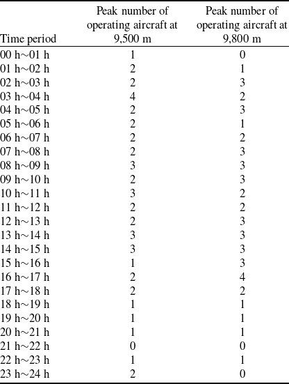
This study selects the AR05 sector of the Guangzhou Area Control in the Central South region as the research object. This sector is a typical example of a high-load, high-density and complex airspace in China, handling nearly a thousand flights daily on average and possesses a complex airspace structure. It not only contains dozens of critical waypoints and intersections but also accommodates multiple high-density routes to and from cities like Beijing and Shanghai. A schematic diagram of the sector is shown in the Fig. 15. This study extracted flight ADS-B data from July 20, 2019 (a typical peak day), and specifically selected data samples from the two most frequently used cruising flight levels: 9,500 m and 9,800 m, to visualise the operation risk within this sector. A sample of the raw Automatic Dependent Surveillance-Broadcast (ADS-B) data is shown in Table 1.
Variation of average risk value and maximum risk value over time.

First, trajectory data preprocessing is performed to address anomalies in raw ADS-B data resulting from environmental interference, signal interruptions and data packet loss. These anomalies are primarily categorised into missing, duplicate and jump trajectory data. Specifically, missing data is characterised by excessive intervals between adjacent points; duplicate data is subdivided into temporal duplicates (multiple points at a single timestamp) and spatial duplicates (identical coordinates across consecutive timestamps); while jump data manifests as outliers between normal trajectory points. To standardise the dataset to 1-s intervals, specific handling strategies are applied. For missing data, no deletion is performed. For temporal duplicates, the average value is calculated. For spatial duplicates, the point corresponding to the median time index is retained. For trajectory jumps, points are identified as outliers and removed if the distance between adjacent points exceeds a dynamic threshold determined by the aircraft’s motion state and time difference. Following data cleaning, the trajectories are interpolated to 1-s intervals. Table 2 statistics show the maximum number of aircraft across all timestamps at the two key flight levels, 9,500 m and 9,800 m, over the entire 24-h period of July 20, 2019. As shown in Table 2, at any given time throughout the day, a maximum of four aircraft were operating simultaneously within the airspace at both the 9,500 m and 9,800 m flight levels. The airspace risk distribution corresponding to the 9,500 m and 9,800 m levels at certain timestamps is shown in Figs 16 and 17.
As illustrated in Figs 16 and 17, the proposed method effectively visualises the spatial distribution of airspace risk alongside the instantaneous positions of aircraft. For all timestamps, 100% of the active ADS-B trajectory points are successfully captured within the identified risk potential zones, with peak intensity values consistently coinciding with the aircraft’s coordinates. This confirms that the model effectively encapsulates individual flight influences within its risk potential field. Notably, the cumulative risk effects resulting from multiple aircraft superimposing their influence on specific spatial points are clearly observable. However, the overall risk values remain at a relatively low magnitude. This is primarily attributed to the sparse traffic density, with a maximum of only four simultaneous aircraft, distributed across the vast geographical extent of the ZGGG AR05 sector.
ADS-B data example

Guangzhou AR05 control sector (a) AR05 airspace structure (b) AR05 sector boundary.

It should be noted that while this ADS-B validation confirms the model’s capability for risk visualisation, it lacks the statistical power required for a rigorous correlation analysis between risk levels and conflict indicators. Conducting such statistical analyses in low-density scenarios with limited sample sizes would yield results lacking statistical significance. Consequently, to rigorously validate the model rationality, a comprehensive evaluation using large-scale simulated traffic flows with higher collision probabilities is presented in the subsequent section.
6.0 Model rationality evaluation
Simulation experiments are established in this section to comprehensively evaluate the model’s performance across varying traffic scales. Specifically, these experiments aim to quantitatively verify the model’s accuracy and explore the complex interrelationships among airspace risk values, aircraft counts, conflict frequency and other key indicators.
Peak number of operating aircraft within various time periods at 9,500 m and 9,800 m

Airspace risk distribution at certain timestamps for the 9,500 m flight level (a) t = 03:08:14 (b) t = 14:00:04 (c) t = 16:17:47.

Aircraft conflict is defined as the distance between two aircraft being less than the specified safety distance. In China, the horizontal safety separation between aircraft is 10 km, and the vertical safety separation is 300 m. The number of conflicts and the conflict rate are chosen as indicators, where conflict rate = the number of conflicts/total number of aircraft, used to measure the intensity of conflicts. To enhance the rationality of the model evaluation, multiple conflict scenarios are designed. The simulation airspace entrance/exit settings are changed from 25 km to 10 km intervals, and the initial route selection method is not changed. The simulation time is set to 0.5 h, with aircraft initial speeds randomly assigned within the range of 800∼1,000 km/h, and the entry times of aircraft into the airspace are randomly distributed. It is also assumed that the aircraft evolves along the predefined route every 1 min. During each evolution, there is a 30% probability that the heading and velocity will change, with heading variations ranging within
 $[ - {30^{^{\circ}}},{30^{^{\circ}}}]$
and speed fluctuations within
 $[ - 0.1{V_{{\rm{current}}}},0.1{V_{{\rm{current}}}}]$
.
The simulation flights are set to be 60, 120, 180 and 240, respectively, to explore the correlation between the risk value of the airspace and each index under different flights. According to the rules, 20 independent simulation experiments are conducted for each traffic volume and recorded every 1 min. These simulations are performed on a workstation equipped with an AMD Ryzen 7 5800H processor (3.20 GHz) and 16 GB of RAM, using MATLAB R2019a as the implementation environment. The distribution of the correlation coefficients between the airspace average risk value and conflict metrics for different flight sorties is shown in Fig. 18.
Airspace risk distribution at certain timestamps for the 9,800 m flight level (a) t = 07:01:22 (b) t = 12:11:22 (c) t = 16:10:48.

Distribution of correlation coefficients. (a) The correlation coefficients between the average risk value and the number of conflicts. (b) The correlation coefficients between the average risk value and the conflict rate.

As shown in Fig. 18, under the scenarios of 60, 120, 180 and 240 flight sorties, the average correlation coefficients between the average risk value and the number of conflicts are 0.64, 0.79, 0.86 and 0.89, respectively, while the average correlation coefficients with the conflict rate are 0.51, 0.69, 0.81 and 0.87, respectively. As the number of sorties increases, the data distribution converges, leading to enhanced stability in the simulation results. These findings demonstrate that a higher aircraft density yields a more consistent and robust correlation between the conflict indicator and the average airspace risk.
In addition, the average correlation between all the indicators in the simulation experiment is calculated, which involves five indicators: average risk value, maximum risk value, the number of aircraft, the number of conflicts and conflict rate. The correlation matrices are plotted as shown in Fig. 19.
Correlation matrix (a) 60 flight sorties (b) 120 flight sorties (c) 180 flight sorties (d) 240 flight sorties.

As shown in Fig. 19, there is a strong correlation between all five indicators. The correlation coefficients between the average risk value and the other four indicators (maximum risk value, the number of aircraft, the number of conflicts and conflict rate) range between 0.5 and 1. As the number of simulated aircraft increases, the average risk value consistently shows a strong correlation with the maximum risk value and the number of aircraft, and the average risk value gradually shows a strong correlation with the number of conflicts and the conflict rate.
Distribution of conflict corresponding to different simulation flights.

To further explore the reason for the lower correlation between the average risk value and conflict indicators in low aircraft simulation experiments compared to high aircraft simulation experiments, the number of conflicts per time unit for different simulation flights is statistically analysed, as shown in Fig. 20.
As can be seen from Fig. 20, when the simulation sorties are 60, 120, 180 and 240, the number of conflicts under each time unit is mainly concentrated in [0, 2], [2, 10], [7, 23] and [13, 40]. The frequency of conflicts per unit time scales significantly with the increase in flight sorties. Specifically, the average conflict counts are 1.55, 6.56, 14.90 and 26.69 for simulation scenarios involving 60, 120, 180 and 240 aircraft, respectively.
When the number of simulated aircraft is relatively low, the number of conflicts remains low and almost unchanged (e.g. [0, 2] for 60 sorties). The correlation relies on the joint fluctuation of the two variables, whereas at lower simulation sorties, the number of conflicts remains almost constant and does not provide enough information to reflect the changing relationship with the average risk value, and, therefore, the corresponding trend between the average risk value and the number of conflicts is weak, resulting in a low correlation. As the number of simulation sorties increases, the number of conflicts rises rapidly and the distribution fluctuation within each time unit increases significantly (e.g. [13, 40] for 240 sorties), creating more synchronised variation between the number of conflicts and the risk value so that stronger correlations are shown at higher simulation sorties.
7.0 Airspace hotspot distribution
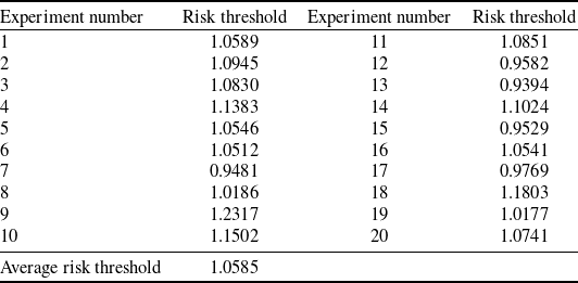
The airspace rasterisation method partitions the airspace into independent grid units, facilitating the calculation of risk values for each grid. Grids with elevated risk values indicate a higher collision probability; thus, identifying the spatial distribution of these high-risk areas provides pilots with a critical reference for trajectory adjustments, enabling autonomous separation maintenance. Following the configuration in preceding sections, all simulations are implemented in MATLAB R2019a on a workstation equipped with an AMD Ryzen 7 5800H processor (3.20 GHz) and 16 GB of RAM. The 80th percentile (0.8 quartile) of grid risk values across all time steps is defined as the risk threshold, with grids exceeding this value labeled as hot grids. The simulation environment spans a 100 km
 $ \times $
100 km area, featuring 60 aircraft over a duration of 0.5 h. The entry and exit points are configured in accordance with Section 5.2. Each aircraft’s predefined route is generated by randomly pairing an entry point with an exit point. Regarding the initial state initialisation, aircraft speeds are randomly assigned within the range of 800∼1,000 km/h, and their entry times into the airspace are stochastically generated. To ensure operational safety, a minimum entry interval of 5 min is enforced for aircraft entering the airspace from the same entry point at the same altitude. For the dynamic evolution process, aircraft update their states along predefined routes every 1 min. During each evolution, there is a 30% probability of adjustments to both heading and speed, with variations constrained within
 $[\! - {30^{^{\circ}}},{30^{^{\circ}}}]$
and
 $[\! - 0.1{V_{{\rm{current}}}},0.1{V_{{\rm{current}}}}]$
, respectively. To analyse risk distribution, three grid size granularities (10 km, 5 km and 1 km) are selected, and the experiment is independently repeated 20 times to determine the risk threshold of this simulated airspace. The calculation results are shown in Table 3. To evaluate the efficiency of the proposed airspace risk modeling method, the average time consumption for calculating grid risks at a single timestamp under different grid scales is recorded. It should be noted that the recorded runtime strictly covers the core computational process of the airspace risk assessment (i.e. from receiving trajectory data to the completion of risk calculation). It excludes the time required for trajectory data loading, grid environment construction and the final visualisation of airspace risk. The results are shown in Table 4.
Therefore, when the risk value of the airspace grid at a certain moment is greater than 1.0585, it indicates that the raster is a hotspot grid, and the on-board auxiliary decision-making system should try to avoid this type of grid when assisting pilots to make trajectory adjustments. Three granularity grid sizes of 10 km, 5 km and 1 km are selected for hotspot visualisation, and the distribution of hotspots in the airspace at a certain moment is shown in Fig. 21.
The risk thresholds for each independent experiment

Average computation time for grid risk at different grid scales

Airspace hotspot distribution (a) 10 km (b) 5 km (c) 1 km.

As can be seen in Fig. 21, airspace grids of different granularity sizes show different details of hotspot distribution. Larger grids (10 km) can capture large-scale hotspot area, while smaller granularities, especially 1 km grids, can more precisely locate hotspots and detect changes in their intensity. Therefore, grids of different sizes are suited to different scenarios. Large-scale grids are suitable for macro-level analysis, quickly identifying large hotspot area; medium-scale grids can better balance the detail and scope of hotspot distribution; and small-scale grids offer high-precision spatial resolution, enabling precise identification of risk distribution. In terms of algorithm computational efficiency, an increase in precision is accompanied by a significant increase in cost. When the grid size is reduced from 10 km to 5 km, the number of grid points increases 4-fold, and the computation time correspondingly increases 3.56-fold. When reduced from 5 km to 1 km, the number of grid points surges 25-fold, and the computation time increases 21.25-fold. This data confirms that the computation time has an approximately linear relationship with the total number of grid points, indicating that the algorithm possesses an efficient O(N) time complexity. Specifically, the average computation times for the three scales are 3.52 ms, 12.54 ms and 266.51 ms, respectively. The 10 km scale (3.52 ms) has an extremely low cost and can be used for autonomous operation scenarios requiring extremely high real-time performance. The 5 km scale (12.54 ms) achieves the optimal balance between precision and efficiency, sufficient to support the smooth, real-time dynamic display of airspace risk hotspots on the airborne side. Conversely, the computation cost of the 1 km scale (266.51 ms) rises sharply. Although not suitable for high-frame-rate display, it offers possibilities for high-precision offline analysis or specific high-risk scenarios. In summary, the airborne decision-support system can flexibly switch grid granularity during autonomous operation based on the mission context. This achieves multi-level airspace safety situation awareness and provides critical support for efficient autonomous operation.
8.0 Conclusions
-
(1) Oriented towards autonomous operation scenarios, this study establishes the influence range of an aircraft’s ellipsoidal risk zone. By integrating the theory of ellipsoidal rotation in 3D space and comprehensively considering aircraft position, speed and heading, a rapid calculation model for risk at any arbitrary point in the airspace is constructed. This model enables the fast computation of grid-based risk at any location, thereby quantifying the airspace safety level and providing data support for flight decision-making.
-
(2) Multi-conflict scenarios are established. By calculating the correlation coefficient between conflict metrics and the average airspace risk value under varying numbers of aircraft, the results demonstrate that with the increase in the number of aircraft, the strong correlation between the conflict indicators and the average risk value of the airspace becomes more stable. This validates the rationality and effectiveness of the proposed method for airspace risk assessment under the autonomous operation mode.
-
(3) Using the airspace rasterisation method, the risk threshold is calculated, and the airspace hotspot distribution is visualised. The differences in hotspot distribution in three grid scales of 10 km, 5 km and 1 km are analysed, which realises the multi-granularity airspace safety situation awareness from the spatial geographic perspective.
-
(4) This study not only enables the visualisation of airspace risk values and hotspot grid distribution from a spatial perspective, but by adjusting the influence range of the ellipsoidal risk zone, it can also achieve airspace risk situation prediction across different time horizons. Regarding the future outlook, several key directions are identified. First, due to the high computational complexity associated with the 3D grid, the current model is primarily simulated and validated during the en-route phase. Future research will optimise the model for complex environments, such as terminal manoeuvring areas where frequent altitude changes occur, thereby enhancing the model’s scalability. Additionally, while this study defines the ellipsoidal risk zone based on fixed parameters, future work will incorporate the heterogeneous performance characteristics of diverse aircraft types under autonomous operations. By constructing dynamic risk zones that conform to specific performance constraints, fine-grained airspace risk assessment will be achieved. Finally, acknowledging that the current real-world validation relies primarily on visual consistency due to the specific low-density timeframe analysed, future work will focus on applying the proposed model to high-density flight data. This will enable rigorous quantitative statistical analyses and model rationality assessments under complex, high-traffic operational conditions.
Author contributions
Shijia Zhang: Writing – review & editing, Writing – original draft, Visualisation, Validation, Methodology, Investigation, Data curation, Conceptualisation. Zhongye Wang: Writing – review & editing, Visualisation, Supervision, Resources, Project administration, Methodology, Conceptualisation. Jia Yi: Writing – original draft, Visualisation. Honghai Zhang: Writing – review & editing, Funding acquisition. Jun Chen: Writing – review & editing.
Competing interests
The authors declared that they have no conflicts of interest in this work.
Data availability statement
Data will be made available on request.
Acknowledgements
The work described in this paper was substantially supported by the Chinese Special Research Project for Civil Aircraft (No. MJZ1-7N22), the National Natural Science Foundation of China (No. U2133207) and the National Social Science Foundation of China (No. 22&ZD169).


 ηl=1
 ηl=2
 ηl=3