2.1. Facilities

The time-resolved PIV experiments were conducted in the low-speed water channel at Beihang University. The schematic of the experimental facilities is illustrated in figure 1(a). A flat and smooth acrylic plate was vertically fixed in the centre of the channel, whose surface served as the wall. This plate measured 200 cm in length, 1.5 cm in thickness and 60 cm in height, protruding from the water with a depth of 50 cm. The ratio of the water depth to the half-width of the flume was 3.33, rendering the flume quite broad in the spanwise direction. An elliptic leading edge with the aspect ratio of $5:1$ was adopted to avoid flow separation from the leading edge of the plate. A slot measuring 402 mm in length and 2 mm in width was reserved 30 cm downstream from the leading edge of the plate, allowing for the unimpeded vertical movement of the fence through it. The non-porous stainless-steel fence, measuring 400 mm in length and 1 mm in thickness, was fixed to the output end of an eccentric drive mechanism. This drive mechanism converted the rotary motion output from the servo motor (Yaskawa SGM7J) into a straight motion along the guide rail via the connecting rod (more clearly visualized in the oblique view from below). The guide rail was fixed above the water channel, and both the motor and the connecting rod can move or be locked in place on the guide rail to adjust the position of the mechanism. The fence was carefully adjusted to fit through the slot, resulting in a height of 10 mm (denoted by $h$ ) between the oscillation centre and the wall. The aspect ratio (width to height) of the fence was 40, sufficient to render the statistics nearly two-dimensional in the vicinity of the fence’s spanwise symmetry centre (Singh et al. Reference Singh, Naughton, Yamashita, Nagai and Asai2011).

Figure 1.

(a) Schematic of the experimental facilities. (b) Schematic of the experimental set-up and FOV for PIV from the spanwise view (not to scale).

The fence was actuated by the eccentric drive mechanism with its oscillation direction perpendicular to the mean shear flow, which facilitates the roll-up of the shear layer and results in apparent modulations on the vortex shedding feature (Singh, Lindberg & Naughton Reference Singh, Lindberg and Naughton2005; Hind, Lindberg & Naughton Reference Hind, Lindberg and Naughton2008). The amplitude ( $A_{{a}}$ ) and frequency ( $f_{{a}}$ ) of oscillation can be controlled by adjusting the eccentric radius and motor speed, respectively. As we are interested in the effect of small perturbations, $A_{{a}}$ was set to be only $0.1h$ . The instantaneous fence height can be expressed as

(2.1) \begin{equation} y_h=A_{{a}}\textrm{sin}(2\pi f_{{a}}t+\varphi _0)+h, \end{equation}

where $\varphi _0$ is the initial phase. It has been demonstrated that the oscillation frequency exhibits a remarkable impact on the vortex shedding characteristics (Miau, Chen & Chou Reference Miau, Chen and Chou1991; Singh et al. Reference Singh, Lindberg and Naughton2005; Hind et al. Reference Hind, Lindberg and Naughton2008). Based on the frequency ratio, $\phi _{{a}} = f_{{a}}/f_{{s}}$ , where $f_{{s}}$ is the natural vortex shedding frequency induced by a stationary fence under identical flow conditions, Singh et al. (Reference Singh, Lindberg and Naughton2005) concluded that flow regimes can be classified into subcritical ( $\phi _{{a}}\lt 0.1$ ), transitional ( $\phi _{{a}}\sim 0.1\text{-}{O}(1)$ ), critical ( $\phi _{{a}}\sim {O}(1)$ ) and supercritical ( $\phi _{{a}}\gt {O}(1)$ ) cases. In the subcritical case, vortices shed at varying frequencies depending on the instantaneous fence height. In the transitional case, unstable vortices are generated where the shedding frequency locks onto $f_{{a}}$ . In the critical case, resonance-enhanced vortices shed at $f_{{s}}$ with intensified vorticity magnitude. In the supercritical case, notably weaker vortices shed at $f_{{a}}$ , and over several oscillation cycles, they coalesce downstream forming larger vortex structures at $f_{{s}}$ . Referring to this conclusion, representative cases covering all flow regimes (see table 1) were examined in the present work to conduct a comprehensive investigation into the influence of oscillation on the TNTI properties. Here, $f_{{s}}\approx 2.0$ Hz, which was obtained from the spectrum in the static case (see § 3.1). In the present experiments, the sampling frequency was sufficiently higher than $f_{{a}}$ , and the total duration of each experiment was much longer than the oscillation period. As a result, the implementation of phase synchronous sampling and the control of $\varphi _0$ were unnecessary.

Table 1.

Oscillation frequencies $f_{{a}}$ and frequency ratios $\phi _{{a}}$ in each case. The terms for flow regimes follow the usage outlined by Singh et al. (Reference Singh, Lindberg and Naughton2005).

2.2. Particle image velocimetry

A brief schematic of the experiment set-up and fields of view (FOVs) for PIV from the spanwise view are shown in figure 1(b). The streamwise, vertical and spanwise directions in the laboratory coordinates are denoted as $x$ , $y$ and $z$ , respectively. The $x$ -axis origin was located at the centre of the slot, and the $y$ -axis origin was located on the wall. The streamwise and vertical instantaneous velocities are denoted by $u$ and $v$ , respectively, the corresponding mean velocities are denoted by $U$ and $V$ , respectively, and the fluctuation components are denoted by $u^\prime$ and $v^\prime$ , respectively. The two-dimensional PIV system was used to obtain the velocity field in the side view section ( $x$ – $y$ plane). Seeding particles were hollow glass beads with a diameter of 5–20 $\unicode{x03BC}$ m and a density of 1.05 g cm⁻ $^3$ , which were illuminated by a laser sheet approximately 1 mm thick generated by a high-frequency double-pulsed laser (Beamtech Vlite-Hi-527). Particle images were synchronously captured by three CMOS cameras ( $2048\times 2048$ pixels) with a sampling frequency of 250 Hz.

The FOVs were located in the central plane of the plate, which were far away from both the water surface and the bottom wall of the channel, thereby allowing for the neglect of the end effect. As demonstrated in previous studies (Li et al. Reference Li, Long and Wang2022; Li & Wang Reference Li and Wang2024), significant changes in the characteristics of the TNTI and entrainment mainly occur in the vicinity of the recirculation zone. In this work, the primary focus is on investigating how oscillations with various frequencies influence the evolution of TNTI characteristics. Therefore, the FOVs were set adjacent to the fence covering the region of $x\in [-2h,24h]$ . The FOV for each camera was approximately 92 mm $\times$ 92 mm ( $9.2h\times 9.2h$ ) and there were overlaps of at least 4 mm (90 pixels) between the FOVs of adjacent cameras. Calibration with a single long reference target covering the entire measurement area was used for stitching all velocity fields together. The multiple iterative Lucas–Kanade algorithm (Pan et al. Reference Pan, Xue, Xu, Wang and Wei2015) was used to calculate the velocity field with an interrogation window of $32\times 32$ pixels and an overlap of 75 % for the final iteration. Following the methods outlined by Qu et al. (Reference Qu, Wang, Feng and He2019), the uncertainties of velocity and vorticity are calculated to be approximately 1.14 mm s⁻¹ and 2.32 s $^{-1}$ , respectively.

Figure 2.

Profile of the mean streamwise velocity for the incoming laminar boundary layer.

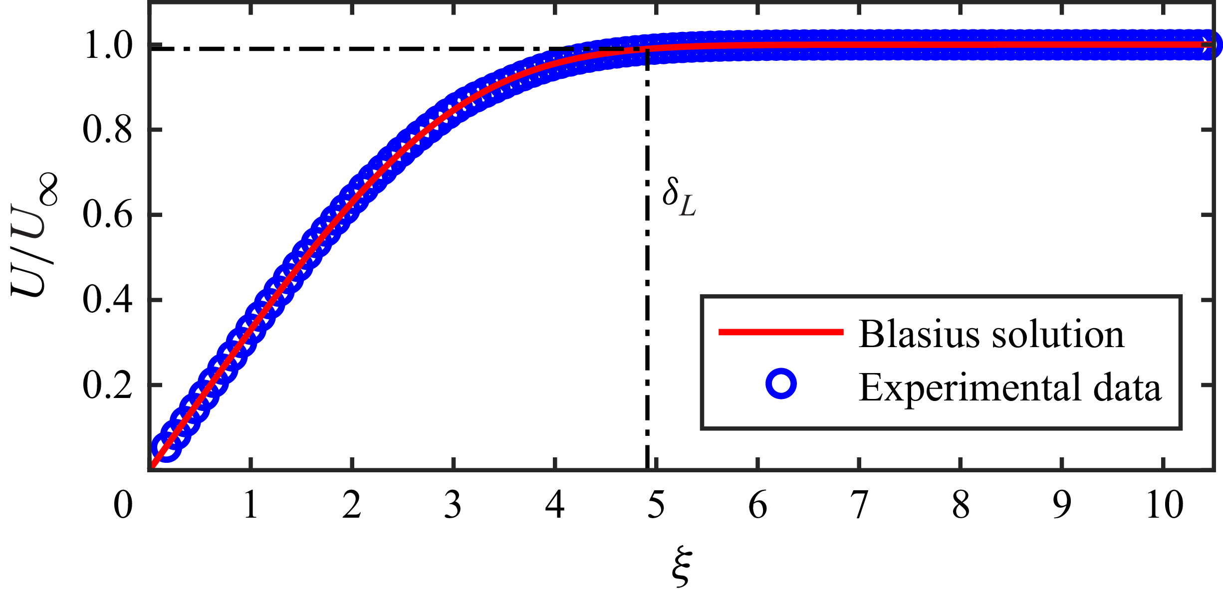
In addition, the incoming boundary layer on the surface of the plate was examined before conducting the formal experiments. Figure 2 shows the profile of the mean streamwise velocity at the location of the slot when the fence was repositioned into the slot (i.e. $y_h=0$ ).The profile matched very well with the theoretical velocity profile of laminar boundary layers – the Blasius solution. The vertical coordinate, $\xi =y\sqrt {U_\infty /\nu x_L}$ , is the dimensionless similarity variable, where $x_L$ is the streamwise distance from the leading edge of the plate and $\nu$ is the kinematic viscosity. The boundary layer thickness $\delta _{L}$ , defined at $0.99U_\infty$ , was $0.83h$ , where the free stream velocity $U_\infty$ was 105 mm s⁻¹. The shape factor $H$ equals 2.59, which aligned well with the theoretical value. The Reynolds number based on the displacement thickness $\delta ^*$ is $Re_{\delta ^*}=U_\infty \delta ^*/\nu =286$ , which is below the critical value ( $Re_{\delta ^*}\leqslant 400$ ) for a laminar boundary layer (White Reference White1991). These results suggested that a stable laminar boundary layer was guaranteed by this experimental set-up.

2.3. Detection of the interface

Generally, turbulent flows have much higher vorticity compared with non-turbulent flows, making the vorticity magnitude (or enstrophy) a prevalent method for detecting the interface between turbulent and non-turbulent regions (da Silva et al. Reference da Silva, Hunt, Eames and Westerweel2014a ). In the present work, the interface is detected by the spanwise component of enstrophy, $\omega _z^2$ . Since the measured enstrophy in the non-turbulent region is not precisely zero due to noise, a threshold, $\omega ^2_{z,{th}}$ , is employed to eliminate the influence of noise. By specifying a threshold, the flow field is divided into two regions: the turbulent region where $\omega ^2_z\gt \omega ^2_{z,{th}}$ and the non-turbulent region where $\omega ^2_z\lt \omega ^2_{z,{th}}$ , as illustrated in figure 3(a). In fact, regions characterized by low enstrophy may also exist within the turbulent region, which are often termed as ‘bubbles’. Nevertheless, bubbles are usually ignored in the detection procedure aimed at identifying the main TNTI due to their infrequent occurrence (Borrell & Jiménez Reference Borrell and Jiménez.2016; Jahanbakhshi & Madnia Reference Jahanbakhshi and Madnia2016; Wu et al. Reference Wu, Wang, Cui and Pan2020). Furthermore, $\omega ^2_{z,{th}}$ is usually determined following an empirical process in which the sensitivity of results to the threshold is tested to obtain an appropriate value (da Silva et al. Reference da Silva, Hunt, Eames and Westerweel2014a ; Zhang et al. Reference Zhang, Watanabe and Nagata2023). Herein, we examined $A_{{T}}/A_{{Tot}}$ against $\omega ^2_{z,{th}}$ as shown in figure 3(b), where $A_{{T}}$ denotes the time-averaged area of the turbulent region and $A_{{Tot}}$ represents the total area of the flow field. Subsequently, the threshold is selected where the gradient $A_{{T}}^\prime$ ( $A_{{T}}^\prime =|\textrm{d}A_{{T}}/\textrm{d}\omega ^2_{z,{th}}|$ ) is minimal, as marked by the hollow circles in figure 3(b).

Figure 3.

(a) Illustration of the turbulent and non-turbulent regions. The solid black curve represents the position of the TNTI. (b) Area ratio $A_{{T}}/A_{{Tot}}$ of the turbulent region and its normalized gradient $A_{{T}}^\prime /A_{{T,max}}^\prime$ as a function of the threshold $\omega ^2_{z,{th}}$ . (c) Conditional averaged enstrophy $\langle \omega _z^2\rangle _{{I}}$ at different streamwise locations in the F20 case.

In addition, the rationality of the interface detection is validated through conditional averaged enstrophy based on the distance from the interface, providing a posteriori corroboration (Jahanbakhshi & Madnia Reference Jahanbakhshi and Madnia2016; Breda & Buxton Reference Breda and Buxton2019; Zhang et al. Reference Zhang, Watanabe and Nagata2023; Su et al. Reference Su, Long, Wang and Li2024). The conditional average method calculates the statistics (denoted as $\langle \boldsymbol{\cdot }\rangle _{{I}}$ ) by averaging the data with the same local TNTI coordinate $y_{{I}}$ at each instant. Here, $y_{{I}}$ originates from the instantaneous TNTI and directs towards the turbulent region, aligning with the local normal direction of the interface, $\boldsymbol{n}=\boldsymbol{\nabla }\omega _z^2/|\boldsymbol{\nabla }\omega _z^2|$ . Consequently, the turbulent and non-turbulent regions are represented by $y_{{I}}\gt 0$ and $y_{{I}}\lt 0$ , respectively. More details of the conditional averaging procedure can be found in our previous works (Li et al. Reference Li, Long and Wang2022; Li & Wang Reference Li and Wang2024). For brevity, only conditional averaged enstrophy $\langle \omega _z^2\rangle _{{I}}$ in the F20 case are presented in figure 3(c). The results show that the interface is well identified, effectively distinguishing the high-vorticity flow from the outer low-vorticity flow with clarity, and clearly capture the step change in enstrophy across the interface at different streamwise locations: in the non-turbulent region outside the interface, $\langle \omega _z^2\rangle _{{I}}$ is nearly zero, while it rapidly increases within the turbulent region.

Strictly speaking, it might be debateable to call this interface the TNTI, given that the separated shear layer is not initially turbulent in some cases. Nevertheless, this detection method is consistent with the procedures for identifying TNTI in fully developed turbulent flows (Zecchetto & da Silva Reference Zecchetto and da Silva2021; Long et al. Reference Long, Wang and Wang2022a ; Xie et al. Reference Xie, Zhang, Xiong and Zhou2024). As the boundary layer evolves farther downstream, this interface will converge to the identical definition of the TNTI in the literature. For simplicity and consistency, the interface herein is also termed as the TNTI following previous practices (Philip et al. Reference Philip, Bermejo-Moreno, Chung and Marusic2015; Long et al. Reference Long, Wang and Wang2022 b).

3.1. Basic flow characteristics

Figure 4(a) shows the mean streamlines around the recirculation zone. Contour lines of $U=0$ and ${\varPhi }=0$ (where $\mathit{\varPhi }(x,y)=\int _0^yU(x,y)\textrm{d}y$ ) are superimposed to estimate the centre and the upper boundary of the separation bubble, respectively (Mohammed-Taifour & Weiss Reference Mohammed-Taifour and Weiss2016; Fang & Tachie Reference Fang and Tachie2019). In the F01 case, the oscillation frequency is very low, causing the characteristics of the mean flow similar to that observed in the F00 (static) case. In the front part of the separation bubble, the flow is predominantly governed by shear motion, while the mean large vortex is located in the latter part of the separation bubble centred at $x\approx 7h$ . It is attributed to the initially laminar nature of the separated shear layer, which develops slowly before the appearance of large-scale shedding vortices (Li & Wang Reference Li and Wang2024). By contrast, when the fence oscillates faster, it prompts the separated shear layer to roll up earlier and form spanwise vortices. As a consequence, the mean large vortices are directly adjacent to the fence, and the flow field characteristics differ qualitatively from those observed in the F00 and F01 cases. The height ( $y_{{r}}$ ) and length ( $x_{{r}}$ ) of the recirculation zone are quantitatively compared by locating the peak point and the intersection with the wall on the contour line of $\mathit{\varPhi }=0$ , respectively. As the oscillation frequency increases, both $x_{{r}}$ and $y_{{r}}$ exhibit a trend of initial decline followed by subsequent increase, attaining their minimum values in the F20 case, as illustrated in figures 4(b) and 4(c), respectively.

Figure 4.

(a) Mean streamlines around the recirculation zone, (b) streamwise length $x_{{r}}$ and (c) vertical height $y_{{r}}$ of the recirculation zone against the oscillation frequency ratio.

To investigate the growth of the separated shear layer in different cases, the streamwise variation of the vorticity thickness is employed as a preliminary indicator. The vorticity thickness is defined as $\delta _{{v}}=(U_{{max}}-U_{{min}})/(\partial U/\partial y)_{{max}}$ , where $U_{{max}}$ and $U_{{min}}$ are the maximum and minimum mean streamwise velocity, respectively, and $(\partial U/\partial y)_{{max}}$ is the maximum vertical gradient of the mean streamwise velocity. It is well known that $\delta _{{v}}$ increases approximately linearly along the streamwise direction in various types of shear layers (Brown & Roshko Reference Brown and Roshko1974; Agelinchaab & Tachie Reference Agelinchaab and Tachie2008; Mohammed-Taifour & Weiss Reference Mohammed-Taifour and Weiss2016). Moreover, recent studies show that its growth rate, $k_{{v}}=\textrm{d}\delta _{{v}}/\textrm{d}x$ , will undergo alternations in response to the transition of the shear layer and the development of flow structures (Fang & Tachie Reference Fang and Tachie2019; Cheng & Chen Reference Cheng and Chen2021; Li & Wang Reference Li and Wang2024).

The variations of $\delta _{{v}}$ affected by the oscillating fence at various frequencies exhibit distinct characteristics. As shown in figure 5(a), in the F01 case, $\delta _{{v}}$ undergoes four discernible stages of development, each characterized by different growth rates $k_{{v}}$ . Within each of these stages, $k_{{v}}$ remains consistent with that observed in the F00 case. This suggests that the evolution of the separated flow in the F01 case is similar to that in the F00 case, with the development of spanwise vortices undergoing several stages: growth ( $0.15x_{{r}}\lt x\lt 0.46x_{{r}}$ ), deformation ( $0.46x_{{r}}\lt x\lt 0.71x_{{r}}$ ) and breakdown ( $x\gt 0.71x_{{r}}$ ), as reported in Li & Wang (Reference Li and Wang2024). Nevertheless, a notable distinction arises in the increase of $\delta _{{v}}$ in the F01 case when $x\lt 0.6x_{{r}}$ , which may be attributed to the undulation of the separated shear layer induced by the oscillation. For an explicit characterization, the instantaneous height of the separated shear layer, $y_{{s}}$ , is measured as the location where the vertical gradient of the instantaneous streamwise velocity ( $\partial u/\partial y$ ) attains its maximum value as shown in figure 6(a). An illustrative example of the temporal fluctuations in the height of the separated shear layer at $x=0.3x_{{r}}$ is presented in figure 6(b). When the fence is static, the height of the shear layer remains relatively consistent. However, when subjected to the forced oscillation, it exhibits sinusoidal variations, resulting in the slight increase in $\delta _{{v}}$ .

Figure 5.

Streamwise variations of vorticity thickness $\delta _{{v}}$ in (a) F00 and F01 cases, (b) F10 and F20 cases, (c) F40 and F60 cases. The black solid line represents the linear fit of vorticity thickness. The growth rate of vorticity thickness is denoted as $k_{{v}}=\textrm{d}\delta _{{v}}/\textrm{d}x$ .

Figure 6.

(a) Visualization of the instantaneous separated shear layer in the F01 case. The red curve marks the height of separated shear layer. (b) Temporal fluctuations of separated shear layer heights at $x=0.3x_{{r}}$ . The black dashed line denotes the mean height in the F00 case, while the black sine curve ( $y_{{s}}/h=0.15\textrm{sin}(2\pi f_{{a}}t+1.44)+1.43$ ) fits the data in the F01 case.

By contrast, in both the F10 and F20 cases, $\delta _{{v}}$ primarily exhibits a linear growth characterized by a uniform growth rate, as depicted in figure 5(b). An exception to this trend is observed in the F10 case, where $\delta _{{v}}$ undergoes nonlinear growth when $x\lt 0.2x_{{r}}$ , indicating a more complex development process during the initial stage of separation. The results indicate a similarity in the evolution of large-scale structures, once they form, within the recirculation zone in these two cases. As the oscillation frequency increases, the growth of $\delta _{{v}}$ exhibits a multistage feature again in the F40 and F60 cases, as shown in figure 5(c). However, due to the earlier formation of spanwise vortices, there are only three development stages characterized by distinct growth rates. Within the range of $0.2x_{{r}}\lt x\lt 0.7x_{{r}}$ , the values of $k_{{v}}$ are equal to 0.21 and 0.20, respectively. They are in close accordance with the results obtained in the F00 and F01 cases when $0.46x_{{r}}\lt x\lt 0.71x_{{r}}$ , as well as with the typical observations ( $k_{{v}}\in [0.15{-}0.22]$ ) reported by previous studies (Brown & Roshko Reference Brown and Roshko1974; Mohammed-Taifour & Weiss Reference Mohammed-Taifour and Weiss2016). This corresponds to the appearance of large-scale vortex structures, which leads to the increase of $k_{{v}}$ . For $x\gt 0.7x_{{r}}$ , $k_{{v}}$ undergoes a decrease analogous to the situation when the fence is static, which might be associated with the breakdown of large-scale vortex structures (Li & Wang Reference Li and Wang2024).

The different evolution processes of the separated shear layer lead to significant changes in the turbulent kinetic energy (TKE) characteristics in the flow field. The TKE is generally defined as $k=({1}/{2})(\overline {u^{\prime 2}}+\overline {v^{\prime 2}})$ for two-dimensional fields. Here, it includes the effects of turbulent fluctuations and periodic changes in velocity caused by oscillation. The distributions of TKE, as well as its streamwise and vertical components, for different cases are presented in figure 7. In the F00 case, the local TKE peak starts its substantial increase only when $x\gt 4h$ . However, in the F01 case, the streamwise turbulent intensity increases significantly before $x\lt 10h$ induced by the oscillation, while the vertical turbulent intensity remains comparable. As a consequence, the local peak of TKE in the F01 case is greater than that in the F00 case when $x\lt 10h$ , while the TKE distributions in both cases become consistent when $x\gt 10h$ . By contrast, in the F10, F20, F40 and F60 cases, the regions of high turbulent intensities become adjacent to the fence, as vortex structures form earlier under the increased oscillation frequency. The global TKE peaks in both the F10 and F20 cases are significantly enhanced with more contributions from their vertical components. This might be related to the existence of stronger and larger-scale shedding vortices in these cases (Hind et al. Reference Hind, Lindberg and Naughton2008). However, when the oscillation frequency further increases in the F40 and F60 cases, the TKE decreases with global peaks even smaller than that when the fence is stationary as a result of the apparent reduction of vertical turbulent intensity. These observations suggest that the shedding vortices are weakened under the high-frequency oscillation.

Figure 7.

Distributions of turbulent intensities in various cases. Panels (i) to (iii) depict the streamwise turbulent intensity ( $\overline {u^{\prime 2}}$ ), vertical turbulent intensity ( $\overline {v^{\prime 2}}$ ) and TKE ( $k$ ), respectively; (a) F00 case, (b) F01 case, (c) F10 case, (d) F20 case, (e) F40 case, (f) F60 case. (g) Streamwise evolution of local peak values of turbulent intensities in all cases. In (a)–(f), solid black lines mark the local peak positions of turbulent intensities; blue dashed and red dot–dashed lines are same as those in figure 4(a), serving as references for the positions of recirculation zones.

To further analyse the dynamic characteristics of the separated flows, the spectra of the vertical fluctuation velocity, $\phi _{v^\prime }$ , are studied under various oscillation frequencies. Here $\phi _{v^\prime }$ is estimated by the Welch method (Welch Reference Welch1967) and normalized by the local variance of vertical velocity. Here, the sequence signals of vertical fluctuation velocity are extracted at the local peaks of the TKE at each streamwise location, as illustrated by black solid lines in figure 7(a), respectively. The signals are divided into four groups following the Welch method, with each group containing 2494 frames, thus determining the frequency resolution as $\Delta f = 250/2494\,\textrm{Hz}\approx 0.1\,\textrm{Hz}$ .

The streamwise evolution of $\phi _{v^\prime }$ under the influence of the oscillating fence is illustrated in figure 8. Here, $St$ is the Strouhal number defined as $St=fh/U_\infty$ . In the F01 case, the evolution of $\phi _{v^\prime }$ generally resembles that observed in the F00 case: there is a discernible frequency migration from high to low frequencies which might be attributed to the complex interaction between vortices at different frequencies (Fang, Tachie & Dow Reference Fang, Tachie and Dow2022). More analyses for the spectrum in the F00 case can be found in our previous work (Li & Wang Reference Li and Wang2024). Nevertheless, there are two apparent differences caused by the oscillation in the F01 case. On the one hand, the prominence of the spectral peak at $St\approx 0.19$ , which corresponds to the natural vortex shedding frequency, becomes diminished and is surpassed by the peaks at $St\approx 0.27$ and $St\approx 0.21$ . This multifrequency instability might be related to the fluctuating instantaneous fence height, which exerts an evident influence on the vortex shedding characteristics in such a quasisteady case (Singh et al. Reference Singh, Lindberg and Naughton2005). On the other hand, a prominent spectral peak can be observed in the vicinity of the fence at the oscillation frequency $St\approx 0.01$ . This peak is associated with the oscillation-synchronized undulation of the separated shear layer as demonstrated in figure 6, which leads to the obvious increase in the vorticity thickness and the TKE as shown above.

Figure 8.

Spectra of vertical fluctuation velocity in each case. The vertical dash–dotted lines indicate the positions of the reattachment points.

By contrast, the effect of oscillation is more remarkable in the F10, F20, F40 and F60 cases. The dominant frequencies in the vicinity of the fence are equal to their own oscillation frequencies (referred to as $St_{{a}}$ hereinafter), respectively, which are associated with the characteristic behaviour that one vortex sheds in each of the oscillation cycles. In the F10 and F20 cases, the flow periodicity is significantly enhanced, with spectral peaks consistently located at $St_{{a}}=0.095$ and $St_{{a}}=0.19$ , respectively, throughout the whole recirculation zone. Notably, the modulation effect of oscillation on the flow is most pronounced in the F10 case, with the dominant frequency being evident across the entire streamwise field of view in the current experiments. The distinct and constant characteristic of the dominant flow frequency in the recirculation zone echoes the phenomenon of constant vorticity thickness growth rate aforementioned, suggesting the formation of relatively stable large-scale motions in the flow field induced by oscillations in both the F10 and F20 cases. By contrast, in the F40 and F60 cases, the frequency migration from high to low frequencies is observed again. Specifically, the predominant spectral peaks in the vicinity of the fence are situated at $St\approx 0.38$ for the F40 case and $St\approx 0.57$ for the the F60 case, respectively. When $x\gt 0.2x_{{r}}$ , the spectral peak gradually shifts from $St_{{a}}$ to $({1}/{2})St_{{a}}$ . Especially, in the F60 case, a weaker secondary frequency migration is noted, resulting in a weak peak at $({1}/{4})St_{{a}}$ . Unlike the behaviour in the F01 case, the frequency migrations here occur at multiples of the foundational frequency. This discrete pattern of frequency migration is typically associated with notable vortex merging (Fang et al. Reference Fang, Tachie and Dow2022), and will be further studied in § 3.2.2.

3.2. Characteristics of vortex structures

Drawing upon the insights into vortex shedding characteristics induced by the oscillating fence, as documented in previous works (Singh et al. Reference Singh, Lindberg and Naughton2005; Hind et al. Reference Hind, Lindberg and Naughton2008; Miau et al. Reference Miau, Chen and Chou1991, Reference Miau, Chen and Chou1995), it can be deduced that the differences in the basic flow characteristics mentioned above are inherently related to variations in the vortex structures. To gain a comprehensive understanding, the characteristics of vortex structures are studied in this section, utilizing the swirling strength ( $\lambda _{{ci}}$ ) criterion (Zhou et al. Reference Zhou, Adrian, Balachandar and Kendall1999) for vortex detection, wherein $\lambda _{{ci}}$ is the magnitude of the imaginary part of the eigenvalue of the velocity gradient tensor. The rotation direction of the vortex structure can be distinguished by the sign of the local spanwise vorticity (Wu & Christensen Reference Wu and Christensen2006; Cui et al. Reference Cui, Pan, Wu, Ye and Wang2019). Then the signed swirling strength is expressed as

(3.1) \begin{equation} \mathit{\varLambda }_{{ci}}=\frac {\omega _z}{|\omega _z|}\lambda _{{ci}}, \end{equation}

and vortices are divided based on their rotation directions into prograde ( $\mathit{\varLambda }_{{ci}}\lt 0$ ) and retrograde ( $\mathit{\varLambda }_{{ci}}\gt 0$ ) vortices.

3.2.1. Generation of the shedding vortex

In the F01 case, the low-frequency fence oscillation does not significantly modulate the vortex shedding characteristics except for small distinctions attributed to the undulation of the separated shear layer. The continuous generation of vortex structures throughout all vertical positions during the undulation of the separated shear layer results in a more dispersed vortex spatial distribution compared with the concentrated organization in the F00 case, as evidenced by the joint PDF (JPDF) of vortex centre coordinates in figure 9(a,b). Here, the vortex centre coordinates, $x_{{c}}$ and $y_{{c}}$ , are defined as

(3.2a) \begin{align} x_{{c}}=\frac {\iint _{\varOmega }{x\mathit{\varLambda }_{{ci}}\textrm{d}\sigma }}{\iint _{\varOmega }{\mathit{\varLambda }_{{ci}}\textrm{d}\sigma }}, \end{align}

(3.2b) \begin{align} y_{{c}}=\frac {\iint _{\varOmega }{y\mathit{\varLambda }_{{ci}}\textrm{d}\sigma }}{\iint _{\varOmega }{\mathit{\varLambda }_{{ci}}\textrm{d}\sigma }}, \end{align}

Figure 9.

(a,b) The JPDF of the centre coordinates, and (c,d) JPDF of the $x$ -coordinates and swirling strength flux of vortex structures in (a) and (c) the F00 case and (b) and (d) the F01 case. Vertical dashed lines are located at $x=0.15x_{{r}}$ , $x=0.46x_{{r}}$ and $x=0.71x_{{r}}$ , respectively, highlighting different evolution stages that correspond to those in figure 5(a).

respectively, where $\varOmega$ denotes the domain of the vortex structure detected by $\lambda _{{ci}}$ criterion and $\textrm{d}\sigma$ is the area element. When the fence is stationary, the shedding vortices exhibit periodicity in their trajectories before they break down, which is reflected by the significant JPDF peak in the figure 9. In contrast, the undulation of the shear layer in the F01 case inclines the shedding vortices to the upper and lower trajectories, resulting in the weak bimodal distribution in the JPDF when $x\lt 0.46x_{{r}}$ . Despite this minor difference, the generation and development of vortex structures in the F01 case generally resemble that in the F00 case which have been systematically studied in our previous works (Li et al. Reference Li, Long and Wang2022; Li & Wang Reference Li and Wang2024). Specifically, the swirling strength flux, which is defined as $J_{\varLambda _{{ci}}}=\iint _{\varOmega }{\mathit{\varLambda }_{{ci}}\textrm{d}\sigma }$ , measuring the strength of the vortex structure, exhibits an identical evolution process in both cases that it undergoes progressive growth for $0.15x_{{r}}\lt x\lt 0.46x_{{r}}$ and tends to attain the peak magnitude in $0.46x_{{r}}\lt x\lt 0.71x_{{r}}$ , as shown in figure 9(c,d).

For the other cases with $\phi _{{a}}\geqslant 0.5$ , the forced oscillations lead to phase-locked vortex shedding, as demonstrated by spectral analysis in figure 8. Therefore, the phase-averaging method is a viable approach for preliminarily studying the vortex shedding characteristics at various fence oscillation frequencies, which has been widely used in previous studies (Miau et al. Reference Miau, Chen and Chou1991; Singh et al. Reference Singh, Naughton, Yamashita, Nagai and Asai2011). However, due to the lack of synchronization between data sampling and the fence oscillation in present experiments, the oscillation phase needs to be obtained by identifying the instantaneous fence height in particle images. As shown in figure 10(a), the particle image is first filtered using a greyscale threshold, and then the greyscale gradient of the images is obtained using the Sobel operator (Woods Reference Woods2011). Finally, the valley line of the greyscale gradient are extracted, which reflects the top edge of the fence. By identifying the top edge of the fence in each frame, the sequence signal of the fence height can be obtained. Subsequently, by fitting this experimentally measured signal to the theoretical positions given by (2.1), the oscillation phase at each time can be determined, as shown in figure 10(b). Afterward, the flow fields are conditionally averaged based on the oscillation phase to obtain the phase-averaged flow fields.

Figure 10.

(a) Procedure of instantaneous height recognition of the oscillating fence. (b) Variation of the instantaneous fence height against the oscillation phase $\varphi$ , where $\varphi =2\pi f_{{a}}t+\varphi _0$ .

Figure 11.

Phase-averaged swirling strength $\tilde {\mathit{\varLambda }}_{{ci}}$ in the (a) F10, (b) F20, (c) F40 and (d) F60 cases. In each subpanel, (i) show the oscillation phase, (ii) show the $\tilde {{\varLambda }}_{{ci}}$ fields, and the black solid lines in (ii) represent the positions of the phase-averaged TNTI height.

When $\phi _{{a}}\geqslant 0.5$ , the oscillations exert considerable influence on the vortex shedding characteristics even with an amplitude of merely 0.1 $h$ . Figure 11 shows the phase-averaged $\tilde {\mathit{\varLambda }}_{{ci}}$ and the phase-averaged TNTI height $\tilde {y}_{{i}}$ . (Here, the instantaneous TNTI height, $y_{{i}}$ , is defined as the vertical distance between the wall and the TNTI.) In the F20, F40 and F60 cases, the vortex shedding exhibits the same pattern as illustrated in figures 11(b), 11(c) and 11(d), respectively. Specifically, vortices accumulate swirling strength in the ascending phase and shed in the descending phase, with these vortices shedding at the oscillation frequency $f_{{a}}$ . These characteristics are consistent with the phenomena observed in previous studies, even though the oscillation amplitude of the fence was larger in those studies (Singh et al. Reference Singh, Lindberg and Naughton2005; Hind et al. Reference Hind, Lindberg and Naughton2008). By contrast, the vortex shedding behaviour in the F10 case is more complex. As shown in figure 11(a), the vortex formed in the ascending phase merges with the vortex formed at the end of the descending phase in the previous cycle. This merged vortex structure experiences a continuous enhancement in swirling strength throughout the ascending phase and sheds when entering the descending phase. In the descending phase, three small shedding vortices are formed sequentially. The first two of them quickly catch up and merge with the vortex generated in the ascending phase, forming a larger-scale vortex structure that moves at $f_{{a}}$ . The third one, however, does not have enough time to shed before entering the next oscillation cycle and merges with the vortex formed in the ascending phase of the next cycle.

In summary, although the oscillation amplitude of the fence in this study is significantly smaller than that in previous studies (Miau et al. Reference Miau, Chen and Chou1991; Singh et al. Reference Singh, Lindberg and Naughton2005; Hind et al. Reference Hind, Lindberg and Naughton2008), the influence of oscillation frequency on vortex shedding characteristics shows highly similar patterns to previous findings. Consequently, the cases in the present study can also be designated as the static, subcritical, transitional, critical and supercritical cases, respectively (see table 1 for precise correspondence). Except for the F01 case where the oscillation has little influence on the vortex shedding, the size of the shedding vortex diminishes as the oscillation frequency rises. Meanwhile, when $\phi _{{a}}\geqslant 1$ , the swirling strength of the shedding vortex decreases with the increase of oscillation frequency. As a consequence, the vortex structure in the F10 case is the largest in scale, while the vortex in the F20 case exhibits the greatest strength. Furthermore, only when the size of the shedding vortices is sufficiently large do they produce a significant modulation effect on the TNTI height. As shown in figures 11(a) and 11(b), evident TNTI height fluctuations emerge in the F10 and F20 cases, with the peaks and troughs associated with the passage and absence of vortex structures beneath the TNTI, respectively. In contrast, the phase-averaged TNTI height shows almost negligible fluctuations in the F40 and F60 cases, resulting from the suppression of the shedding vortex under higher-frequency oscillations.

3.2.2. Development of the shedding vortex

In view of the aforementioned results in § 3.1, it is evident that there are complex development processes of vortex structures farther downstream which exhibit significant differences in various cases. In summary, three distinct development situations can be observed.

The first situation exists in the subcritical case (specifically the F01 case), where the flow statistical characteristics remain largely similar to that observed when the fence is stationary (the F00 case), suggesting that the low-frequency oscillation has a more pronounced effect on prompting the undulation of the separated shear layer rather than the vortex-shedding dynamics. Therefore, the conclusion outlined in our previous work (Li & Wang Reference Li and Wang2024) remains applicable: based on changes in the growth rate of vorticity thickness (see figure 5 a), the evolution of the separation shear layer can be quantitatively divided into stages such as the laminar shear layer ( $0\lt x\lt 0.15x_{{r}}$ ), vortex formation and growth ( $0.15x_{{r}}\lt x\lt 0.46x_{{r}}$ ), large-scale deformation of the vortex ( $0.46x_{{r}}\lt x\lt 0.71x_{{r}}$ ) and vortex breakdown ( $x\gt 0.71x_{{r}}$ ).

The second situation occurs in the supercritical cases including the F40 and F60 cases, where the vorticity thickness also exhibits multiple stages of development with different growth rates and the spectra exhibit apparent discrete frequency migrations. These discrete frequency migrations are usually associated with vortex merging, which can be can be demonstrated more intuitively with the wavelet analysis. Wavelets are helpful in studying periodic characteristics of time series associated with time-varying frequencies. The wavelet spectrum is computed based on the Morlet wavelet (Morlet Reference Morlet1983), which shows the effectiveness in analysing time–frequency characteristics of separated flows (Wang & Wang Reference Wang and Wang2021). Figure 12(a) presents the results for the F60 case at $x=2h$ ( $x\approx 0.2x_{{r}}$ ), where high wavelet coefficients are alternately clustered around three frequencies: $St_{{a}}$ , $({1}/{2})St_{{a}}$ and $({1}/{4})St_{{a}}$ . From the wavelet spectrum, the typical instants at which these characteristic frequencies emerge can be caught, thereby allowing for a comparison of flow features at the corresponding moments.

Figure 12.

(a) Wavelet spectrum of vertical fluctuation velocity at $x=2h$ in the F60 case. Panels (b)–(e) show the instantaneous ${\varLambda }_{{ci}}$ fields at $\varphi \approx 183.4\pi$ , $\varphi \approx 118.4\pi$ , $\varphi \approx 121.0\pi$ and $\varphi \approx 122.7\pi$ , respectively. Here ‘ $\textrm{V}_i$ ’ ( $i$ = 1, 2, 3, …) represents successively shedding vortex structures, with the sum of subscript numbers indicating vortex merging.

Figure 12(b) shows a typical flow field when $({1}/{2})St_{{a}}$ dominates, where the two shedding vortices $V_1$ and $V_2$ undergo pairing and merging, resulting in a shift of the dominant frequency from $St_{{a}}$ to $({1}/{2})St_{{a}}$ . Figure 12(c–e) illustrate the formation mechanism of $({1}/{4})St_{{a}}$ : after vortex structures $\textrm{V}_1$ and $\textrm{V}_2$ merge to form $\textrm{V}_{1+2}$ , they continue to attract and merge with the third ( $\textrm{V}_3$ ) and fourth ( $\textrm{V}_4$ ) vortex structures. Although the vortex structure generated after the merging with $\textrm{V}_3$ soon breaks down, the small-scale vortices formed as a result still move around a centre (as indicated by the dashed circle in figure 12 e), and attract $\textrm{V}_4$ to merge with it. As a side note, the emergence of $({1}/{4})St_{{a}}$ does not involve a scenario where vortex structures first pair and merge in pairs and then merge again. If $\textrm{V}_3$ and $\textrm{V}_4$ had merged first, they would have maintained the flow state corresponding to $({1}/{2})St_{{a}}$ . Additionally, the spectral peak corresponding to the inherent vortex shedding frequency when the fence is stationary does not appear in the F60 case, because the phenomenon observed in previous studies (Singh et al. Reference Singh, Lindberg and Naughton2005) that multiple vortex structures shedding at the oscillation frequency merge into a large-scale vortex moving at the inherent frequency does not occur in the present experiment. It may be related to the different oscillation modes of the fence: in previous studies, when the amplitude was larger, the fence will retreat into the wall, whereas in this study, the amplitude is smaller and the fence always remains above the wall.

Furthermore, the regions where spectral peaks appear at $({1}/{2})St_{{a}}$ in the F40 case and at $({1}/{2})St_{{a}}$ and $({1}/{4})St_{{a}}$ in the F60 case generally coincide with the range where the vorticity thickness growth rate $k_{{v}}$ increases, respectively. It suggests that the variation of $k_{{v}}$ within $0.2x_{{r}}\lt x\lt 0.7x_{{r}}$ is related to the pairing and merging behaviour of vortex structures. Consequently, based on variations in vorticity thickness growth rate (see figure 5 c), the flow evolution process can also be quantitatively divided into stages such as vortex formation and growth ( $0\lt x\lt 0.2x_{{r}}$ ), vortex pairing and merging to form large-scale structures ( $0.2x_{{r}}\lt x\lt 0.7x_{{r}}$ ) and breakdown of large-scale structures ( $x\gt 0.7x_{{r}}$ ). It is noteworthy that, although the increase in vorticity thickness growth rate is closely related to the formation of large-scale vortex structures in both subcritical and supercritical cases, the formation processes differ: in the subcritical case, the formation of large-scale vortex structures is associated with the secondary instability of the spanwise vortex leading to the large-scale deformation; while in the supercritical cases, the generation of large-scale vortex structures is attributed to pairing and merging of the small shedding vortices.

The third situation encompasses the transitional (F10) and critical (F20) cases, where vortices have a relatively large size upon shedding. In these cases, the vorticity thickness growth rate is unique within the recirculation zone, and the dominant frequency remains constant. However, instantaneous flow field visualization (see figure 13) reveals that these large-scale vortex structures break down before the flow reattachment. To statistically characterize the evolution of shedding vortices and establish basic understanding on the flow feature in this situation, the JPDFs of vortex structure size, $R_{{v}}$ (measured as $R_{{v}}=\sqrt {A_{{v}}/\pi }$ where $A_{{v}}$ is the area of the vortex structure detected by $\lambda _{{ci}}$ criterion), and vortex centre height, $y_{{c}}$ , in the F10 and F20 cases are investigated as presented in figures 14(a) and 14(b), respectively.

Figure 13.

Sequential visualization of the shedding vortex breakdown in the (a) F10 case and (b) F20 case. Here $t_1$ and $t_2$ represent the starting moments of these two examples, respectively. The time interval is one quarter of the oscillation period for both cases. The black solid curves show the instantaneous TNTI locations, while the black dashed lines highlight the correspondence of shedding vortices. The boundaries of prograde and retrograde vortices are marked by blue and red curves, respectively, except for the breaking vortices which are highlighted with magenta boundaries.

Figure 14.

The JPDFs of vortex size $R_{{v}}$ and vortex centre height $y_{{c}}$ in the (a) F10 and (b) F20 cases. Here $R_{{v}}\lt 0$ corresponds to prograde vortices, while $R_{{v}}\gt 0$ represents retrograde vortices. The black horizontal dashed line indicates the height of the local peak of TKE.

When $x\lt 0.5x_{{r}}$ , the motion of the shedding vortex exhibits a good periodicity, with vortices of similar size tending to follow similar trajectories, which is reflected in the JPDF as significant probability peak regions. In the F10 case, the large-scale structure consists of the central large vortex and peripheral small vortices, but the centre-to-centre spacing between them is relatively large, and vortex merging is incomplete. Therefore, two independent peak regions can be observed in the JPDF as indicated by the red arrows in figure 14(a). Such a structure is inherently unstable, exhibiting stronger three-dimensional characteristics (Singh et al. Reference Singh, Lindberg and Naughton2005). In contrast, the vortex structure core is unique in the F20 case, thus there is only one concentrated peak region in the JPDF.

When $x\gt 0.5x_{{r}}$ , the aforementioned peak regions gradually disappear. This phenomenon is not caused by a weakening of flow periodicity (as evidenced in figure 8) but reflects the breakdown of vortex structures. Although the small-scale vortex structures generated after breakdown still move around the centre, their sizes are more diverse and their spatial distribution is dispersed, leading to the disappearance of peak regions in the JPDF. As a consequence, the flow evolution process in these two cases can be roughly divided into the formation and growth of large-scale vortices ( $x\lt 0.5x_{{r}}$ ) and the breakdown of the large-scale structure ( $x\gt 0.5x_{{r}}$ ).

4.1. Distribution of the TNTI height

Figure 15 presents the streamwise variations of the first two statistical moments of the TNTI height, namely, the mean value, $Y_{{i}}$ , and the standard deviation, $\sigma _{{i}}$ , both normalized by the local boundary layer thickness, $\delta$ . Despite of the presence of higher $\sigma _{{i}}$ compared with the F00 case as a result of the enhancement of the low-frequency undulation of the separated shear layer induced by oscillation, the streamwise evolution of the TNTI height statistics in the F01 case exhibits a process similar to that in the F00 case. These results are caused by the similar evolution processes of vortex structures in these two cases. Specifically, when $x\gt 0.46x_{{r}}$ , $Y_{{i}}/\delta$ begins decreasing while $\sigma _{{i}}/\delta$ gradually increases, associated with the large-scale deformation of the shedding vortex due to secondary instability. When $x\gt 0.71x_{{r}}$ , the shedding vortex breaks down into numerous small-scale vortex structures, leading to more rapid changes in both $Y_{{i}}$ and $\sigma _{{i}}$ .

Figure 15.

Streamwise variations of the mean and standard deviation of the TNTI height.

For cases with oscillation frequency ratios of $\phi _{{a}}\geqslant 0.5$ , vortex structures form earlier, causing significant changes in the TNTI height statistics after $x\gt 0.2x_{{r}}$ . Especially, there are periodically strong large-scale vortex structures in the initial stages of separation in both the F10 and F20 cases, which present the same impact mechanism on the TNTI height. Therefore, $Y_{{i}}$ and $\sigma _{{i}}$ for these two cases coincide well with each other initially. However, after the breakdown of the large-scale vortices ( $x\gt 0.5x_{{r}}$ ), differences begin to appear between these two cases. In the F10 case, the size of flow structures is larger, causing $\sigma _{{i}}$ to further increase and $Y_{{i}}$ to diminish faster compared with those in the F20 case. Overall, for cases with $\phi _{{a}}\geqslant 0.5$ , $Y_{{i}}$ increases in the recirculation zone as the oscillation frequency increases, while the change in $\sigma _{{i}}$ is the opposite.

Moreover, the streamwise variations of the PDFs of the TNTI height $y_{{i}}$ in different cases are illustrated in figure 16. In the F00 case, the separated shear layer is initially laminar, leading to the symmetric and sharply peaked PDF (Li & Wang Reference Li and Wang2024). In contrast, the oscillating fence enhances the TNTI height fluctuations, manifested as the reduced peak value and broader distribution of PDF. Although the mean value and standard deviation of the TNTI height exhibit almost identical evolution in the F00 and F01 cases, their PDFs show different evolution processes. A bimodal distribution can be found in the F01 case at the early stage of separation, which reflects the sinusoidal undulation of the separated shear layer as illustrated in figure 6. This phenomenon is expectable, as the PDF of a perfect sinusoidal signal exhibits bimodality, with two peaks corresponding to the maximum and minimum displacement positions, respectively. The TNTI fluctuates in response to the undulation of the separated shear layer, therefore exhibiting this bimodal distribution.

Figure 16.

The PDFs of the TNTI height at different streamwise positions.

Furthermore, another distinct bimodal distribution can be observed near $x=0.8x_{{r}}$ in the F00 case. The dominant peak corresponds to the elevated TNTI when vortex structures pass through, while the secondary peak reflects the TNTI trough due to the induction of the local intense downwash flow generated by the strong prograde vortex typically appearing at $x\approx 0.6x_{{r}}$ as shown in figure 9(c). In contrast, this secondary peak is absent in the F01 case, which might be related to the undulation of the shear layer. To be more specific, when the shear layer displaces to the lower position, the formation of large-scale vortices is suppressed, thereby reducing the strong downwash required to generate the TNTI troughs. Conversely, when the shear layer undulates upward, the TNTI is elevated as a whole. Therefore, the probability density of trough occurrence at the same height has significantly decreased.

For cases with $\phi _{{a}}\geqslant 0.5$ , the PDF of the TNTI height begins to apparently varies as the shedding vortices form when $x\gt 0.2x_{{r}}$ , with its distribution gradually shifting towards the inner region of the boundary layer closer to the wall. By contrast, in the F00 and F01 cases, the PDF of the TNTI height appearing closer to the wall gradually increases only after the occurrence of large-scale deformation of the vortex structure. In terms of overall variation, in the F00, F01 and F10 cases ( $\phi _{{a}}\lt 1$ ), the PDF of the TNTI height evolves from a sharply peaked distribution to a positively skewed one. However, in the F20, F40 and F60 cases ( $\phi _{{a}}\geqslant 1$ ), the PDF of the TNTI height remains basically symmetric.

However, although differences in TNTI height distributions are apparent within the recirculation zone due to distinct vortex structure characteristics induced by the oscillating fence at different frequencies, the PDFs of TNTI heights in different cases gradually converge to two distinct distributions when $x\gt 1.2x_{{r}}$ . Similarly, the streamwise evolution of $Y_{{i}}$ and $\sigma _{{i}}$ also converge to two curves. Specifically, the F00, F01 and F10 cases constitute one group, where the TNTI height fluctuations are prominent, and the PDFs of TNTI height exhibit a significant positive skewness, with lower $Y_{{i}}$ ( $0.51\delta$ ) and larger $\sigma _{{i}}$ ( $0.28\delta$ ). In these cases, the large-scale shedding vortices exhibit greater spatial separation. Their induced downwash flow promotes the formation of troughs in the TNTI profile. As these primary vortices break down into smaller vortex structures, which consist of clusters maintaining relatively large intercluster spacing as exemplified by the instantaneous fields in the F01 and F10 cases in figure 17, the TNTI troughs become further amplified, resulting in substantial height fluctuations of the TNTI. Meanwhile, the TNTI trough depth is physically constrained by the wall-attached shear layer thickness, whereas the TNTI peak height remains unbounded by such flow boundaries. This asymmetric behaviour leads to the characteristic positive skewness observed in the TNTI height distribution.

Figure 17.

Distribution of the instantaneous vortex structures and TNTI in different cases. The locations of the TNTI are indicated by the black lines.

Conversely, the F20, F40 and F60 cases consist of the other group, where higher-frequency oscillations attenuate both the strength and size of the shedding vortices, thereby reducing their induction effects. This results in a more compact spatial distribution of vortex structures, as exemplified by the F20 and F40 cases in figure 17. As a consequence, the TNTI height exhibits diminished fluctuations with higher $Y_{{i}}$ ( $0.62\delta$ ) and smaller $\sigma _{{i}}$ ( $0.24\delta$ ). The height PDFs in this group maintain a symmetric distribution as the peaks and troughs of the TNTI are hardly constrained by the wall.

Notably, the evolution of TNTI height distribution in the F10 case is the most special. Before the breakdown of large-scale structures ( $x\lt 0.5x_{{r}}$ ), the variation trends in the PDF of TNTI height, $Y_{{i}}$ , and $\sigma _{{i}}$ are similar to those observed in the F20 case. However, after the breakdown of large-scale vortex structures, the statistical characteristics of the TNTI height exhibit different trends and ultimately converge with the characteristics observed in the F00 and F01 cases. Studies on the distribution of the TNTI height at different oscillation frequencies reveal that, during the initial stage of separation, the distribution of the TNTI height is significantly influenced by the size of the dominant vortex structure. However, after the breakdown of large-scale vortex structures, it depends more on the spatial distribution of vortex structures.

4.2. Dynamic properties of the TNTI

Dynamic properties of the TNTI typically involve the flow characteristics in the vicinity of the TNTI. Generally, the TNTI is characterized by a significant step change of vorticity magnitude near the TNTI (da Silva et al. Reference da Silva, Hunt, Eames and Westerweel2014a ), which occurs in a thin layer known as the TNTI layer. The mean thickness of the TNTI layer, $\delta _\omega$ , is quantified as the distance from the TNTI to the location where $\langle |\omega _z|\rangle _{{I}}^\prime /[\langle |\omega _z|\rangle _{{I}}^\prime]_{{max}} = 0.2$ in this work, as described in figure 18 with the F20 case serving as an example. Here, $\langle |\omega _z|\rangle _{{I}}^\prime$ is the gradient of the conditional averaged vorticity $\langle |\omega _z|\rangle _{{I}}$ against the TNTI coordinate $y_{{I}}$ (i.e. $\langle |\omega _z|\rangle _{{I}}^\prime =\textrm{d}\langle |\omega _z|\rangle _{{I}}/\textrm{d}y_{{I}}$ ) and $[\langle |\omega _z|\rangle _{{I}}^\prime]_{{max}}$ is its maximum value. To investigate the streamwise evolution of the dynamic TNTI properties, profiles of $\langle |\omega _z|\rangle _{{I}}$ at different streamwise positions are stitched together to provide a more intuitive representation, as shown in figure 19. The TNTI thickness $\delta _\omega$ and the positions of peak values are superimposed in the figures denoted by solid and dashed black lines, respectively.

Figure 18.

Definition of the mean TNTI thickness at $x=2x_{{r}}$ in the F20 case. Here $\eta _{{I}}$ denotes the Kolmogorov scale whose definition is provided in Appendix A.

Figure 19.

Conditional averaged vorticity in different cases. The black solid lines indicate the TNTI thickness defined by $\langle |\omega _z|\rangle _{{I}}^\prime =0.2[\langle |\omega _z|\rangle _{{I}}^\prime]_{{max}}$ , and the black dashed lines indicate the peak of the conditional average vorticity.

In the F01 case, the distribution of $\langle |\omega _z|\rangle _{{I}}$ is generally consistent with that in the F00 case where the fence is stationary. Prior to the occurrence of large-scale deformation of the shedding vortex ( $x\lt 0.46x_{{r}}$ ), the flow near the TNTI is dominated by shear motion. Both the position of the peak value of $\langle |\omega _z|\rangle _{{I}}$ and $\delta _\omega$ change little along the streamwise direction, and they coincide well with each other. When $x\gt 0.46x_{{r}}$ , the mean shear weakens, and the peak value of $\langle |\omega _z|\rangle _{{I}}$ begins to decrease. After the breakdown of the shedding vortices ( $x\gt 0.71x_{{r}}$ ), $\langle |\omega _z|\rangle _{{I}}$ decreases more rapidly, and its peak value moves closer to the TNTI.

In the F10 and F20 cases, flows dominated by shear motion also exist in the close vicinity of the fence, where $\delta _\omega$ coincides with the peak position of $\langle |\omega _z|\rangle _{{I}}$ and gradually decreases. After the formation of shedding vortices, due to their large scale, the distribution of $\langle |\omega _z|\rangle _{{I}}$ is significantly affected, resulting in the peak position of $\langle |\omega _z|\rangle _{{I}}$ to move away from the TNTI. In the F40 and F60 cases, the size of the shedding vortices decreases, and the evolution process of $\langle |\omega _z|\rangle _{{I}}$ is similar to that in the F00 and F01 cases to some degree. However, due to the earlier generation and evolution of vortex structures, $\langle |\omega _z|\rangle _{{I}}$ begins to decay earlier. The streamwise evolution of $\delta _\omega$ exhibits different patterns affected by the oscillating fence at various frequencies. In the F01, F40 and F60 cases, $\delta _\omega$ initially remains approximately constant and then gradually decreases to reach a new constant value, which is consistent with the behaviour when the fence is stationary. By contrast, $\delta _\omega$ decreases monotonically in the F10 case, while it undergoes increases and decreases in the F20 case.

To further study the development of the TNTI thickness, $\delta _\omega$ is compared with two characteristic length scales. One is the distance from the TNTI to the centre of the separated shear layer ( $\varDelta _{{s-I}}$ ) as illustrated in figure 20(a), in view of the dominance of the fluid shear motion at the early stage of flow separation. The other is the radius of the adjacent vortex structures ( $\overline {R}_{{v}}$ ), whose boundaries are explicitly marked in figure 20(b), motivated by the finding that the TNTI thickness typically scales with the size of nearby vortices in the fully developed turbulence (Silva & Taveira Reference da Silva and Taveira2010; Silva et al. Reference Silva, Zecchetto and da Silva2018). The streamwise evolution of $\delta _\omega$ , $\varDelta _{{s-I}}$ and $\overline {R}_{{v}}$ is presented in figure 21. On the one hand, the evolution of $\delta _\omega$ in different cases shows some similarities: $\delta _\omega$ initially coincides with $\varDelta _{{s-I}}$ , indicating that shear motion dominates the flow at the initial stage of separation. It reveals that the step change in vorticity is essentially the increase of vorticity from the external free stream towards the centre of the separated shear layer. Besides, after the reattachment, $\delta _\omega$ remains almost constant matching the scale of the vortex structure closest to the TNTI ( $\delta _\omega \approx 1.6\overline {R}_{{v}}$ herein), which reflects the similarity of TNTI dynamic characteristics after the flows become turbulent. On the other hand, apart from these common characteristics, there are also notable differences in the evolution of $\delta _\omega$ in various cases. In the F00 and F01 cases, the mean shear begins to weaken after the large-scale deformation of vortex structures ( $x\gt 0.46x_{{r}}$ ). Consequently, $\delta _\omega$ decreases as the vortex structures diminish in size before the flow reattachment. Similarly, the reduction in $\delta _\omega$ in the F40 and F60 cases is associated with the decline in the mean shear. Notably, in the F60 case with a higher oscillation frequency, $\delta _\omega$ reaches a constant value earlier. It might be attributed to the more complex vortex-merging phenomena in this case, which lead to the earlier formation of small-scale vortex structures near the TNTI. In contrast, the evolution of $\delta _\omega$ in the F10 and F20 cases is more complex, with a shorter streamwise region dominated by fluid shear motion. In addition, the subsequent development of $\delta _\omega$ does not exhibit a clear correlation with the evolution of $\varDelta _{{s-I}}$ and $\overline {R}_{{v}}$ .

Figure 20.

(a) Illustration of the instantaneous distance $\varDelta _{{s-I}}$ between the TNTI and the separated shear layer centre. (b) Visualization of vortices adjacent to the TNTI, with prograde and retrograde vortices marked by blue and red curves, respectively. Both snapshots are extracted from the F01 case.

Figure 21.

Streamwise variation of the TNTI thickness $\delta _\omega$ , the mean distance $\varDelta _{{s-I}}$ from the TNTI to the centre of the separated shear layer and the mean radius $\overline {R}_{{v}}$ of the vortex structure closest to the TNTI. Here, $\overline {R}_{{v}}$ is multiplied by 1.6 for clearer comparison.

To gain a deeper understand of the evolution of TNTI thickness in the F10 and F20 cases, the JPDFs of $R_{{v}}$ and $\varDelta _{{v-I}}$ at different locations are examined as illustrated in figure 22 and figure 23, respectively. Here, $\varDelta _{{v-I}}$ denotes the shortest distance from the vortex centre $(x_{{c}},y_{{c}})$ to the TNTI, as illustrated in figure 20(b). As mentioned in § 3.2.2, the large-scale vortex structure in the F10 case is composed of a central large vortex surrounded by smaller vortices. Due to the relatively large distance between these two components, the JPDF exhibits two comparable peak regions before the breakdown of the large-scale structure as shown in figure 22, where $\delta _\omega$ (marked by the dashed lines) remains associated with the distance between the small-scale structures and the TNTI. In contrast, in the F20 case, the large-scale vortex structure possesses a prominent single centre with considerable strength. Although it also induces shear motion and small-scale vortices rotating around it, these induced structures are weaker or too close to the large one. Therefore, in the F20 case, the evolution of $\delta _\omega$ in the recirculation zone is always related to the distance between the large-scale vortex structure and the TNTI, as shown in figure 23. However, subsequent to the breakdown of the large-scale vortex structures after the flow reattachment, the evolution of $\delta _\omega$ exhibits the same pattern that becomes associated with the distance between the TNTI and the adjacent small-scale vortex structures regardless of the initial conditions.

Figure 22.

The JPDFs of vortex size $R_{{v}}$ and the distance $\varDelta _{{v-I}}$ from the vortex centre to the TNTI in the F10 case. Here $R_{{v}}\lt 0$ corresponds to prograde vortices, while $R_{{v}}\gt 0$ represents retrograde vortices.

Figure 23.

The JPDFs of vortex size $R_{{v}}$ and the distance $\varDelta _{{v-I}}$ from the vortex centre to the TNTI in the F20 case. Here $R_{{v}}\lt 0$ corresponds to prograde vortices, while $R_{{v}}\gt 0$ represents retrograde vortices.

Furthermore, the streamwise variations of the characteristic scale of $\delta _\omega$ are studied by comparing $\delta _\omega$ with the local Kolmogorov scale $\eta _{{I}}$ and the Taylor microscale $\lambda _{{I}}$ (definitions are provided in Appendix A) as shown in figures 24(a) and 24(b), respectively. Except for the monotonically decreasing $\delta _\omega /\eta _{{I}}$ downstream of the fence in the F10 case, $\delta _\omega /\eta _{{I}}$ for the other cases is significantly increased in the recirculation zone. The TNTI thickness is significantly larger than the Kolmogorov scale in the recirculation zone. For the F00, F01, F40 and F60 cases, the maximum value of $\delta _\omega$ can reach $25\eta _{{I}}$ to $30\eta _{{I}}$ , while for the F20 case, its maximum value even reaches approximately $45\eta _{{I}}$ . In contrast, throughout the evolution process, $\delta _\omega$ is consistently of the order of the Taylor microscale. After the breakdown of large-scale vortex structures, the non-dimensionalized TNTI thicknesses for different cases converge to the uniform value, attributed to the fact that the TNTI thickness is determined by the size of small-scale vortex structures near the TNTI (Silva & Taveira Reference da Silva and Taveira2010; Silva et al. Reference Silva, Zecchetto and da Silva2018). Specifically, $\delta _\omega$ converges to approximately $10\eta _{{I}}$ or $0.5\lambda _{{I}}$ , which is consistent with previous observations in fully developed turbulent flows (Chauhan et al. Reference Chauhan, Philip, de Silva, Hutchins and Marusic2014a ; Watanabe et al. Reference Watanabe, Sakai, Nagata, Ito and Hayase2014, Reference Watanabe, da Silva, Sakai, Nagata and Hayase2016).

Figure 24.

Streamwise variation of the TNTI thickness non-dimensionalized by (a) the local Kolmogorov scale $\eta _{{I}}$ and (b) the local Taylor microscale $\lambda _{{I}}$ .

5.1. Effects of oscillation on engulfment

As the engulfment mechanism will lead to the formation of low-vorticity bubbles, quantitative analysis of engulfment can be conducted by focusing on these structures. Bubbles are extracted using the same method and threshold as those employed for the TNTI detection, with noise points smaller than $3\times 3$ grid points being filtered out. The low-vorticity regions within the recirculation zone can be also identified as bubbles. However, they are isolated from the external free stream by the separated shear layer, which are thus unrelated to the engulfment mechanism. Furthermore, bubbles can also form within the turbulent region (da Silva et al. Reference da Silva, Hunt, Eames and Westerweel2014b ), which are not associated with engulfment as well. To distinguish between bubbles originating from engulfment and those generated within the turbulent region, the method, which differentiates the bubbles based on their distance ( $\varDelta _{{b-I}}$ ) to the TNTI, is commonly employed by previous studies (Jahanbakhshi & Madnia Reference Jahanbakhshi and Madnia2016; Long et al. Reference Long, Wang and Wang2022a ; Xu et al. Reference Xu, Long and Wang2023). In this work, based on the characteristics of the fluctuation velocity within the bubbles, the TNTI thickness $\delta _\omega$ serves as the threshold for $\varDelta _{{b-I}}$ to distinguish various bubbles. Specifically, when $\varDelta _{{b-I}}\lt \delta _\omega$ , the fluctuation velocity within the bubbles increases significantly as $\varDelta _{{b-I}}$ increases. Conversely, when $\varDelta _{{b-I}}\gt \delta _\omega$ , the fluctuation velocity within the bubbles remains constant or decreases slightly. More details can be found in our previous work (Li & Wang Reference Li and Wang2024).

Subsequently, the contribution of the engulfment mechanism to entrainment is quantitatively evaluated through the time-averaged engulfment flux per unit streamwise length, denoted as $\overline {F}_{{e}}$ (Li & Wang Reference Li and Wang2024). Local $\overline {F}_{{e}}$ within a streamwise window of width $L_x$ is calculated by summing the areas ( $A_{{b}}$ ) of the bubbles in the TNTI layer within that window, and then dividing the sum by the total time duration $T$ and the window length, i.e.

(5.1) \begin{equation} \overline {F}_{{e}}=\frac {1}{T}\frac {1}{L_x}\sum _{\varDelta _{{b-I}}\lt \delta _\omega } A_{{b}}. \end{equation}

To investigate the streamwise evolution of the engulfment mechanism, $\overline {F}_{{e}}$ at different locations is obtained by sliding the window along the streamwise direction. Additionally, $L_x$ is set to be $1h$ in the present work. Slight variations in $L_x$ do not qualitatively affect the conclusions, while a larger $L_x$ would result in a smoother streamwise evolution of $\overline {F}_{{e}}$ at the cost of reduced spatial resolution. Additionally, before summing the areas of the bubbles, the advective trajectories of bubbles are tracked, and only the first-appearing bubble on each trajectory is retained to avoid double-counting the same bubble from a Lagrangian perspective.

The streamwise variations of $\overline {F}_{{e}}$ in various cases are illustrated in figure 25. In the F01 case, the engulfment process becomes evident subsequent to the breakdown of the shedding vortex. Here $\overline {F}_{{e}}$ rapidly increases prior to reattachment, induced by the strong downwash flow in the reattaching region. However, its growth slows down after the reattachment, due to the absence of induction from strong downwash flow. This result aligns well with observations in the F00 case where the fence is stationary. In contrast, higher-frequency oscillations prompt the earlier formation of large-scale vortex structures, leading to an earlier onset of the engulfment mechanism. In the F10 and F20 cases, $\overline {F}_{{e}}$ exhibits a process of initial increase, subsequent decrease and then another increase, with a remarkable enhancement in the vicinity of the reattachment point. The vortex structures are the strongest in the F20 case, inducing a more intense downwash flow. As a consequence, $\overline {F}_{{e}}$ appears the earliest and attains the highest peak value compared with all other cases. In the F10 case, vortex structures are relatively large and can induce intense downwash flow as well, resulting in the second-largest magnitude of $\overline {F}_{{e}}$ among the other cases.

Figure 25.

Streamwise variations of the time-averaged engulfment flux $\overline {F}_{{e}}$ affected by the oscillating fence at different frequencies. The vertical dotted lines show the reattachment points of the corresponding cases (indicated by the same colour), respectively.

However, in the F40 and F60 cases, as the downwash flow is weakened due to the decreased strength of the shedding vortices, $\overline {F}_{{e}}$ exhibits the smaller value with the increase of the oscillation frequency. Moreover, the higher oscillation frequency will result in the later emergence of the engulfment process. In the F40 case, $\overline {F}_{{e}}$ rapidly increases before flow reattachment and then grows more slowly thereafter, whose variation trend is similar to that in the F00 case. In contrast, in the F60 case, the growth rate of $\overline {F}_{{e}}$ remains essentially constant before and after the reattachment, and its magnitude is already lower than that measured in the F00 case where the fence is stationary. It may be attributed to high-frequency oscillations promoting an increase in the number of shedding vortices, leading to a denser spatial distribution of vortex structures and thereby significantly inhibiting the effect of the engulfment mechanism.

5.2. Effects of oscillation on nibbling

The movement of the TNTI can be decomposed into two components: the advection with the local flow and the displacement caused by local nibbling. Thus, nibbling is usually quantified by the entrainment velocity $v_{{n}}$ , which is calculated by subtracting the local advection from the total movement per unit time. Due to the lack of three-dimensional data in this work, $v_{{n}}$ is obtained utilizing the TNTI-tracking method proposed by Wolf et al. (Reference Wolf, Lüthi, Holzner, Krug, Kinzelbach and Tsinober2012), which has been employed in many previous studies based on two-dimensional data sets (Mistry et al. Reference Mistry, Philip, Dawson and Marusic2016; Kankanwadi & Buxton Reference Kankanwadi and Buxton2020; Long et al. Reference Long, Wang and Wang2022a ). More details about the calculation procedure of $v_{{n}}$ can be found in our previous work (Li & Wang Reference Li and Wang2024). In addition, note that negative $v_{{n}}$ represents the expansion of the turbulent region (corresponding to the entrainment process) because the TNTI normal vectors are oriented from the non-turbulent region to the turbulent region herein.

The streamwise variations of the time-averaged entrainment velocity $\overline {v}_{{n}}$ and the root-mean-square (superscript rms) of the entrainment velocity $v_{{n}}^{{rms}}$ are illustrated in figure 26. Both of these quantities are non-dimensionalized by the local Kolmogorov velocity scale, which is defined as $u_\eta =(\nu \varepsilon _{{I}})^{1/4}$ herein. It has been demonstrated that prograde vortices near the TNTI tend to cause a significant reduction in the mean entrainment velocity, while retrograde vortices exhibit the opposite behaviour (Li & Wang Reference Li and Wang2024). Consequently, the minimum magnitude of $\overline {v}_{{n}}/\eta _{{I}}$ aligns with the presence of the strong large-scale prograde vortices in all cases, coinciding well with the peak location of the mean swirling strength flux, $\overline {J}_{\varLambda _{{ci}}}$ , for the vortex structures closest to the TNTI, as shown in the inset of figure 26(a). The evolution of $\overline {v}_{{n}}/\eta _{{I}}$ can be divided into two groups depending on when the shedding vortex forms. In the F00 and F01 cases, the minimum magnitude of $\overline {v}_{{n}}/\eta _{{I}}$ is observed at $x\approx 0.55x_{{r}}$ . By contrast, as the shedding vortex forms earlier for cases where $\phi _{{a}}\geqslant 0.5$ , the minimum magnitude of $\overline {v}_{{n}}/\eta _{{I}}$ is attained soon at $x\approx 0.15x_{{r}}$ .

Figure 26.

Streamwise variations of (a) the time-averaged entrainment velocity $\overline {v}_{{n}}$ and (b) the root-mean-square of entrainment velocity $v_{{n}}^{{rms}}$ in different cases. The inset in (a) shows the evolution of the mean swirling strength flux $\overline {J}_{\varLambda _{{ci}}}$ of vortex structures closest to the TNTI.

Besides, it is noteworthy that, unlike the swirling strength of vortex structures, the minimum magnitude of $\overline {v}_{{n}}/\eta _{{I}}$ does not exhibit significant variations in different cases. This may be due to the fact that the influence of vortex structures on entrainment velocity depends not only on the vortex strength but also on the distance from the vortex structure to the TNTI (Watanabe et al. Reference Watanabe, Jaulino, Taveira, da Silva, Nagata and Sakai2017a ). The increase in vortex structure size also results in the vortex structures being farther away from the TNTI. After the breakdown of the shedding vortex, the entrainment velocity continues to increase and reaches its peak in the rough vicinity of $x=1.2x_{{r}}$ in all cases. This uniformity supports the previous conclusion that the increase in entrainment velocity is related to the induction by the downwash flow associated with the reattachment, instead of the promotion of retrograde vortices (Li & Wang Reference Li and Wang2024). Additionally, the peak value of $\overline {v}_{{n}}/\eta _{{I}}$ tends to increase first and then decrease as the oscillation frequency increases, attaining the maximum in the F20 case.

On the other hand, the variations of entrainment velocity fluctuations also exhibits some similarities among different cases, as shown in figure 26(b). In the F01 case, similar to the F00 case, $v_{{n}}^{{rms}}/\eta _{{I}}$ is small in the initial stage of separation and remains relatively constant. It then begins to increase significantly after the large-scale deformation of the vortex structures, reaching a maximum at the reattachment point, followed by a gradual decay thereafter. For the cases where $\phi _{{a}}\geqslant 0.5$ , the shedding vortices form earlier, leading to an earlier onset of the increase in $v_{{n}}^{{rms}}/\eta _{{I}}$ . Except for the F60 case where has the oscillation frequency is very high, all other cases exhibit a maximum value of $v_{{n}}^{{rms}}/\eta _{{I}}$ near the reattachment point, followed by a decay to $v_{{n}}^{{rms}}\approx 2\eta _{{I}}$ . In the F60 case, $v_{{n}}^{{rms}}/\eta _{{I}}$ reaches its maximum value $v_{{n}}^{{rms}}\approx 2\eta _{{I}}$ at $x=0.6x_{{r}}$ and remains basically constant thereafter. This may be related to the smallest scale and strength of the shedding vortices in the F60 case, resulting in a weakened fluctuation of the entrainment velocity.

Figure 27.

(a) Streamwise variations of the time-averaged nibbling flux $\overline {F}_{{n}}$ . (b) Streamwise variations of the contribution percentage by the engulfment mechanism.

Furthermore, the fluid volume entrained by the nibbling mechanism is jointly determined by the entrainment velocity and the curve length of the TNTI (Mistry et al. Reference Mistry, Philip, Dawson and Marusic2016; Long et al. Reference Long, Wang and Wang2022a ). Therefore, to quantify the contribution of the nibbling mechanism to entrainment, the nibbling flux is investigated which is defined as

(5.2) \begin{equation} F_{{n}}=\frac {1}{L_x}\int _{\textit{TNTI}} v_{{n}}\textrm{d}s, \end{equation}

where $\textrm{d}s$ is the length element along the TNTI curve. The streamwise evolution of the dimensionless time-averaged nibbling flux, $\overline {F}_{{n}}/\eta _{{I}}$ , in various cases is presented in figure 27(a). Here $\overline {F}_{{n}}/\eta _{{I}}$ exhibits a similar variation trend with $\overline {v}_{{n}}/\eta _{{I}}$ along the streamwise direction. This strong similarity further supports the previous conclusion that, in the separated and reattaching flows, the evolution of the entrainment velocity – rather than the increase in the interfacial contact area with the free stream caused by the TNTI distortion – plays a dominant role in the evolution of the nibbling flux (Li & Wang Reference Li and Wang2024). Moreover, when $\phi _{{a}}\geqslant 1$ , $\overline {F}_{{n}}/\eta _{{I}}$ will diminish against the increase of the oscillation frequency. It can be attributed to the fact that as the oscillation frequency rises, the shedding vortices become smaller in size and more compact in spatial distribution, resulting in a reduction in both the entrainment velocity and the tortuosity of the TNTI. Finally, the contribution of engulfment mechanisms to the total entrainment is quantitatively assesses by comparing $\overline {F}_{{e}}$ and the total entrainment flux ( $|\overline {F}_{{n}}|+\overline {F}_{{e}}$ ). Figure 27(b) shows the proportion of $\overline {F}_{{e}}$ to the total entrainment flux. Generally, although oscillation at an appropriate frequency (e.g. at $\phi _{{a}}=1$ ) can significantly enhance the engulfment flux, its magnitude remains substantially smaller than that of the nibbling flux. In the recirculation zone, the proportion of the engulfment flux is always less than 6 %.