





Introduction
Greenland and Antarctica are the world’s largest store of freshwater ice, with the potential to become the main drivers of sea-level rise (De Conto and Pollard, Reference De Conto and Pollard2016; Mouginot and others, Reference Mouginot2019). Subglacial water plays a key role in determining how the ice sheets slide over their bases, and hence how much ice is transported to regions where melting is enhanced—the ocean or lower altitudes (Iken and Bindschadler, Reference Iken and Bindschadler1986; Clarke, Reference Clarke1987; Schoof, Reference Schoof2010; Hewitt, Reference Hewitt2013; Bougamont and others, Reference Bougamont, Christoffersen, Hubbard, Fitzpatrick, Doyle and Carter2014; Flowers, Reference Flowers2015). Yet, ice-sheet-scale models struggle to include dynamic subglacial hydrology (Flowers, Reference Flowers2015; Sommers and others, Reference Sommers, Rajaram and Morlighem2018; Kazmierczak and others, Reference Kazmierczak, Gregov, Coulon and Pattyn2024), resulting in uncertainties in sea-level rise predictions (Feldmann and Levermann, Reference Feldmann and Levermann2015; Pörtner and others, Reference Pörtner2019; Zoet and Iverson, Reference Zoet and Iverson2020). Although the most sophisticated models now attempt to include some drainage elements (e.g. channels) (e.g. De Fleurian and others, Reference De Fleurian2018; Sommers and others, Reference Sommers2024; Ehrenfeucht and others, Reference Ehrenfeucht, Dow, McArthur, Morlighem and McCormack2025), due to the large range of length scales involved, 1 m to  $10^{5}\,\mathrm{m}$, ongoing work is needed to find a consistent physical model that describes these subglacial and englacial networks (Warburton and others, Reference Warburton, Meyer and Sommers2024), which can then be upscaled or implemented in ice-sheet-scale simulations.
At the base of glaciers and ice sheets, sufficiently large flows of water are observed to carve out channels, which are significant conduits of meltwater to the ocean. Röthlisberger was the first to posit that at every cross-section of a drainage channel, there exists a local balance between outward melting of the channel walls and the inward viscous collapse of the surrounding ice—as much ice is melted as flows in (Röthlisberger, Reference Röthlisberger1972; Walder, Reference Walder2010). Viscous dissipation (frictional heating) in the flowing water causes the ice–water boundary to melt, while the viscous flow of ice due to overburden stresses drives channel collapse or closure. Röthlisberger’s model assumed a circular cross-section for the channel, which allowed the use of Nye’s analytic expression to describe the closure rate of the channel (Nye, Reference Nye1953). In this formulation, the closure rate is driven by the effective pressure,  $N$, defined as the difference between the ice overburden pressure,
 $p_i$, and the water pressure within the channels,
 $p_w$ (
 $N = p_i - p_w$). Conversely, the melting power is given by the product of the volumetric flux,
 $q$, and the pressure gradient,
 $G$. The theoretical treatment of these variables involves a distinction in regard to the primary external drivers: while Röthlisberger’s analysis focuses on the steady-state relationship between
 $N$ and
 $q$, later extensions by Walder and Fowler (Reference Walder and Fowler1994) and Ng (Reference Ng2000) emphasise
 $G$ as a largely constant driver dictated by the regional ice-surface slope and bed topography. Using this model, Röthlisberger derived relationships between pressure gradients driving the flow and the resulting volumetric flow rates, providing evidence of subglacial water preferentially flowing in larger channels than in distributed, sheet-like flow. Walder and Fowler (Reference Walder and Fowler1994) and subsequently Ng (Reference Ng2000) expanded this framework to account for other subglacial drainage elements—notably canals incised into deformable subglacial sediment—with fundamentally different pressure-flux relationships.
Theoretical investigations into non-circular englacial and non-semicircular subglacial channels have been motivated by observational evidence and model predictions. Water pressures in subglacial channels are frequently observed to be higher than reasonably predicted by circular channels (Iken and Bindschadler, Reference Iken and Bindschadler1986; Hooke and others, Reference Hooke, Laumann and Kohler1990), and more recent direct observations of non-circular channel cross-sections with large aspect ratios have been made (Church and others, Reference Church, Grab, Schmelzbach, Bauder and Maurer2020; Kamintzis and others, Reference Kamintzis2023). Furthermore, many sophisticated subglacial network models break down for very thin and tall channels and predict ever-narrowing channels, suggesting an underlying drive towards more eccentric cross-sections (Hewitt, Reference Hewitt2011; Sommers and others, Reference Sommers, Rajaram and Morlighem2018).
Motivated by higher-than-previously-predicted observed water pressures, Hooke and others (Reference Hooke, Laumann and Kohler1990) modelled subglacial channels as low and broad (the arc of a circle forming the ice ceiling and its chord as the bedrock base). This new channel shape required higher pressure gradients to drive the same amount of flux, providing an explanation for the higher water pressures. Fowler and Ng (Reference Fowler and Ng1996) considered a subglacial channel cross-section in the shallow limit of great width and very low ceilings—the ice-roof and bedrock-bottom boundaries were treated as parallel. More recent models have been proposed for non-circular cross-sections due to variations in the viscous collapse of the ice. Meyer and others (Reference Meyer, Fernandes, Creyts and Rice2016) showed that initially circular channels can be deformed into either broader or taller channels due to anti-plane shearing within the ice, for example, near shear margins or under surging glaciers. If the ice surrounding a channel experiences shearing (vertical or horizontal variation in the downstream velocity), there is a local variation in the viscosity of the ice, causing an initially circular or semicircular channel to deform. Dallaston and Hewitt (Reference Dallaston and Hewitt2014) considered the stability and shape evolution of channels without making any a priori assumptions about their cross-sections. By approximating the ice rheology as Newtonian and modelling the meltwater as a uniform heat source that filled the cavity, they demonstrated that the simple contraction of a circular cavity is unstable to perturbations in the channel shape, and instead ellipses provide an exact and stable solution, provided their aspect ratios are sufficiently close to unity. Though their work provides a framework to better understand the observational evidence of non-circular channel cross-sections, they note the limitation of their uniform heating model and speculate that non-uniform melting along the interface, due to its geometry, may result in new stable, non-circular cross-sections.
In this work, we model the flow of water through the channels to derive a spatially variable melt rate along the perimeter of the channels’ ice–water interface. Furthermore, we extend Röthlisberger’s model to include elliptical channels, which allows for a variation in the aspect ratio of the channels. We consider melting caused by both laminar and turbulent flow and introduce a hybridised laminar–turbulent melt model, resulting in stable elliptical cross-sections. We examine the resulting pressure-flux relationships of these stable channels, revealing that channels with elliptical cross-sections, beyond a critical flux threshold, tend to share flux similar to that of a distributed drainage network. This behaviour contrasts with circular channels, which undergo channelisation towards fewer, larger channels. Finally, the implications and limitations of this work are discussed in the broader context of ice flow models.
Mathematical model and approach
We consider an elliptical englacial channel that is uniform in the along-flow ( $x$) direction and is connected to a water source providing a constant volume flux to the channel. We assume that the channel grows in cross-section only due to melt-back of the ice, driven by viscous dissipation in the flow of water that fully fills the channel. The viscous dissipation in the flow produces a temperature profile, which is then used to calculate a spatially varying melt rate along the channel wall. We further assume that the channel closure is due only to the viscous collapse of the surrounding ice, which is modelled using Newtonian Stokes flow.
We first consider the limit of laminar flow in the channel and subsequently consider turbulent flow. Thereafter, we find the temperature profile for the laminar and separately the turbulent flow, before considering the resulting melt at the ice–water boundary. We then bring together the two types of melting by proposing a hybrid laminar–turbulent melting scheme, which captures flow in small and large channels and in those with high aspect ratios. This hybrid melting is combined with the viscous collapse of the channel to determine stable cross-sectional aspect ratios and areas.
Flow through the channel
The flow in the channel is driven by a pressure gradient,  $G\equiv -\text{d}p/\text{d}x$, with a constant input volume flux,
 $q$. We assume gravity plays a negligible role in determining the flow inside the channel, and that a quasi-steady state exists where the interface melts back slowly, with the flow adjusting quickly to new cross-sections, so that a time-independent description is sufficient. We assume the water, with viscosity
 $\eta_w$, experiences a no-slip condition at the channel boundary. The channel is restricted to the shape of an ellipse with horizontal semi-axis,
 $a$, and vertical semi-axis,
 $b$, in the
 $y$ and
 $z$-directions, respectively; see Fig. 1. We define its aspect ratio as
 $\xi = b/a$.
 $\Omega$ denotes the interior of the ellipse with an area,
 $A= \pi ab$, and
 $\partial \Omega$ defines its boundary.
Schematic representation of an elliptical englacial channel: The water flows into the page and is surrounded by ice. The red outward normal arrows represent melting driven by viscous dissipation, and the blue varying inward normal arrows represent the collapse due to viscous collapse of the surrounding ice.

Laminar flow
For small channels with little volume flux, the flow is laminar and unidirectional and the Reynolds number,
 \begin{equation}
\text{Re} = \frac{\rho_w U L}{\eta_w},
\end{equation}
where  $\rho_w$ denotes the density of water and
 $U$ and
 $L$ are the characteristic velocity and length scales, is small. In the limit
 $\text{Re}\ll 1$, this flow is described by the Stokes equation,
 \begin{equation}
\nabla^2 u = - \frac{G}{\eta_w} \quad \text{in} \;\Omega,
\end{equation}
 \begin{equation}
u = 0 \quad \text{on} \; \partial \Omega.
\end{equation}
This has a known solution (Happel and Brenner, Reference Happel and Brenner1983) for the water velocity
 \begin{equation}
u = \frac{G a^2 b^2}{2 \eta_w (a^2 + b^2)}\left( 1- \frac{y^2}{a^2}-\frac{z^2}{b^2} \right),
\end{equation}
which we use to find the volumetric flux,
 \begin{equation}
q = \frac{G}{4\pi\eta_w}\frac{\xi}{\xi^2+1}A^2,
\end{equation}
written here in terms of the cross-sectional area  $A$ and the aspect ratio
 $\xi$ of the channel. Figure 2a shows the scaled flow field through a channel with an aspect ratio of
 $\xi = 1/2$.
Flow and temperature profiles for laminar and turbulent flows through an ellipse with aspect ratio  $\xi = 1/2$: Velocity profile for laminar (a) and turbulent (b) flows are normalised to a maximal value of one. The turbulent boundary layer thickness,
 $\delta$, is also labelled. The normalised temperature profiles for laminar (c) and turbulent (d) flow include scaled and coloured arrows representing heat flux into the boundary. All contours match the labels on the colour bar.

Figure 2 Long description
Panel a shows a contour plot of normalised velocity for laminar flow in an elliptical cross-section. The vertical axis is labeled z and the horizontal axis is labeled y, with arbitrary units . Dashed contour lines indicate smooth gradients across the section. Panel b displays normalised velocity for turbulent flow, with a nearly uniform core and a thin near-wall layer. The vertical axis is labeled z and the horizontal axis is labeled y, with arbitrary units . The color bar labeled u ranges from 0 to 1, representing normalised velocity magnitude. An expression for boundary layer thickness, delta approximately equals eta subscript w Re subscript c over rho subscript w U, is annotated near the boundary. Panel c shows normalised temperature for laminar flow with arrows indicating outward wall flux direction. The vertical axis is labeled z and the horizontal axis is labeled y, with arbitrary units. Panel d presents normalised temperature for turbulent flow, showing a more uniform core. The color bar labeled T ranges from 0 to 0.995 and another color bar labeled v ranges from 0.27 to 1, representing normalised wall-normal velocity or heat-flux-related quantity. Arrows around the boundary indicate heat flux direction, with color encoding magnitude. The turbulent case highlights a thin boundary layer and more uniform core compared to the laminar case.
These descriptions may be made non-dimensional, and we choose to scale both these solutions and subsequent turbulent and hybrid solutions in the following way. The dimensions of the ellipse are scaled differently in the two principal directions,  $y \sim a$ and
 $z \sim b$, and the velocity is scaled by the average flow speed
 $u\sim u_{av} = q/A$. The scaled boundary is therefore a circle
 \begin{equation}
\tilde{y}^2 + \tilde{z}^2 = 1,
\end{equation}
and the scaled Poisson equation, (3), describing the flow in the channel becomes
 \begin{equation}
\xi^2 \frac{\partial^2 \tilde{u}}{\partial \tilde{y}^2} + \frac{\partial^2 \tilde{u}}{\partial \tilde{z}^2} = -4(\xi^2 + 1),
\end{equation}
which has solution
 \begin{equation}
\tilde u = 2(1-\tilde{y}^2-\tilde{z}^2).
\end{equation}
The geometric influence of the elliptical cross-section for laminar flow can therefore be entirely accommodated by the rescaling of the principal axes and the introduction of  $\xi$ to the governing equation. This scaling and notation facilitate the subsequent analysis of the temperature field.
Turbulent flow
In the turbulent limit, we expect a non-linear relation between the volume flux and the applied pressure gradient. We can show this by arguing that the mean turbulent flow  $U$ is surrounded by a thin laminar boundary layer of width
 $\delta$ along the perimeter,
 $P$, of the channel cross-section, see Fig. 2b. The width of the boundary layer can be approximated by assuming that the local Reynolds number at the laminar boundary is at its critical value,
 \begin{equation}
\text{Re}_c = \frac{\rho_w U \delta}{\eta_w} \simeq 10^3.
\end{equation}
The resistive force to bulk flow is assumed to be from the viscous boundary layer only  $\sim\!{P} \eta_wU /\delta $. The water flows due to the force from the pressure gradient acting across the entire cross-sectional area
 $A$. Balancing the driving and resistive forces gives
 \begin{equation}
\eta_w \frac{U}{\delta}P \simeq GA.
\end{equation}
If we rearrange this expression and substitute for the boundary layer width, we find that
 \begin{equation}
G = \frac{1}{\text{Re}_c}\frac{P}{A}\rho_w U^2.
\end{equation}
This is equivalent to the empirically derived Darcy–Weisbach equation (Weisbach, Reference Weisbach1850),
 \begin{equation}
G \equiv - \frac{\text{d}p}{\text{d}x} = f_D \frac{\rho_w U^2}{2D_H},
\end{equation}
where, by convention,  $D_H \equiv 4A/P$ is termed the hydraulic diameter and
 $f_D \sim 1/\text{Re}_c$ is the friction factor. We note, in general, that the value of
 $f_D$ in the turbulent limit depends on several factors, including, for example, the relative roughness of the channel. Here, we shall assume that
 $f_D \sim 10^{-3}$ as in Hewitt and others (Reference Hewitt, Chini and Neufeld2018). It is possible to define a friction factor in the laminar case, and then go on to combine the flow regimes into a hybridised flow scheme using a friction factor that depends on the Reynolds number, see, for example, (Churchill, Reference Churchill1973; Hewitt and others, Reference Hewitt, Chini and Neufeld2018). We refrain from doing so here because a hybrid flow formulation is unable to resolve the variations in heat flux along the boundary and therefore cannot predict how the channel’s geometry might be altered by melting.
The hydraulic diameter,  $D_H$, measures the dominant length scale in the flow problem, tending to the smaller semi-axis,
 $a$ or
 $b$, in the limit of large or small aspect ratio, respectively. The area of an ellipse has a simple expression,
 $A =\pi a b = \pi\xi a^2 $, but its perimeter is given by
 \begin{equation}
P = 4a E[1-\xi^2],
\end{equation}
where  $E$ is the complete elliptic integral of the second kind,
 $E[1-\xi^2] \equiv \int_{0}^{{\pi}/{2}} \sqrt{1 - (1-\xi^2) \, \sin^{2}\theta} \, \text{d}\theta$. The hydraulic diameter is therefore given by
 \begin{equation}
D_H = \frac{\pi\xi a}{E[1-\xi^2]}.
\end{equation}
This is the characteristic length scale used to define a Reynolds number for the flow in the elliptical conduit,
 \begin{equation}
\text{Re} = \frac{\rho_w D_H U}{\eta_w},
\end{equation}
which we will use later to determine whether the flow through the channels is laminar or turbulent.
Temperature fields
The water’s viscosity results in the dissipation of energy, releasing heat. The flow profile determines where this heat is produced and subsequently where melting occurs. The gradient of the temperature field along the boundary sets the heat flux into the boundary and hence determines how much melting occurs. Outside the channel and on the boundary, the ice is assumed to be at the ice’s melting temperature,
 \begin{equation}
T = T_m \quad \text{on } \partial \Omega.
\end{equation}
This provides the boundary condition for the temperature profile.
Laminar
For steady laminar flow of an incompressible fluid of constant thermal conductivity,  $k_T$, heat conduction balances the heat generated by viscous dissipation (Landau and Lifshitz, Reference Landau and Lifshitz1987), so that
 \begin{equation}
- k_T \nabla^2 T = \eta_w \left[ \left( \frac{\partial u}{\partial y} \right)^2 + \left( \frac{\partial u}{\partial z} \right)^2 \right].
\end{equation}
We non-dimensionalise using the same scalings as in the flow problem,  $y \sim a$,
 $z \sim b$,
 $u\sim u_{av} = q/A$, and scaling the temperature field,
 $T$ by
 \begin{equation}
T_0 = \frac{\eta_w u_{av}^2}{k_T},
\end{equation}
such that  $T = T_m+ T_0 \tilde{T}$. Hence, the heat equation (17), becomes
 \begin{equation}
\xi^2 \frac{\partial^2 \tilde{T}}{\partial \tilde{y}^2} + \frac{\partial^2 \tilde{T}}{\partial \tilde{z}^2}= - \left[ \xi^2 \left( \frac{\partial \tilde{u}}{\partial \tilde{y}} \right)^2 + \left( \frac{\partial \tilde{u}}{\partial \tilde{z}} \right)^2 \right].
\end{equation}
The known solution to  $\tilde{u}$, (8), can be substituted into this equation to obtain
 \begin{equation}
\nabla_{\xi}^2 \tilde{T} = -16 (\xi^2\tilde{y}^2+\tilde{z}^2) \quad \text{in} \; \Omega,
\end{equation}
 \begin{equation}
\tilde{T} = 0 \quad \text{on} \; \partial\Omega.
\end{equation}
Note that the above equation depends only on the aspect ratio  $\xi$. We can solve for the temperature field using a quartic ansatz,
 \begin{equation}
\tilde{T} = \left( \tilde{y}^2+\tilde{z}^2-1\right)\left(A\tilde{y}^2 + B\tilde{z}^2 +C \right),
\end{equation}
that meets the boundary condition and mirrors the symmetry of the problem. The unknown coefficients are found by substituting into (20) and matching coefficients,
 \begin{equation}
A = \frac{4\left(1-6\xi^2-\xi^4\right)}{3\left(1+6\xi^2+\xi^4\right)},
\end{equation}
 \begin{equation}
B = -\frac{4\left(1+6\xi^2-\xi^4\right)}{3\left(1+6\xi^2+\xi^4\right)},
\end{equation}
 \begin{equation}
C =-\frac{4\left(1+4\xi^2+\xi^4\right)}{3\left(1+6\xi^2+\xi^4\right)}.
\end{equation}
The resulting rescaled solution for the temperature field for an ellipse where  $\xi = 1/2$ is shown in Fig. 2c. For the no-slip boundary condition to be met in the laminar flow problem, more shear is required along the shorter semi-axis. This increased shear leads to more heat production, and hence to more melting along this shorter axis, driving evolution of the ellipse towards
 $\xi = 1$.
Turbulent
In the turbulent limit, we expect a turbulent, well-mixed and thermally uniform interior surrounded by a thin laminar boundary layer, which has the same depth,  $\delta$, everywhere (Schlichting and Gersten, Reference Schlichting and Gersten2017), see Fig. 2b. We follow the Reynolds analogy by assuming that in this turbulent limit, heat and momentum are mixed by the same mechanisms, with the Prandtl number approaching unity, and hence the thermal and velocity boundary layer thicknesses are the same (Reynolds, Reference Reynolds1874).
We do not attempt to resolve the averaged temperature profile in an elliptical channel but argue that for a constant thickness boundary layer, with a temperature difference  $\Delta T$ across the layer, the heat flux into the ice, given by
 $\boldsymbol{F}_H \simeq \hat{\boldsymbol{n}} k_T \frac{\Delta T}{\delta}$, where
 $\hat{\boldsymbol{n}}$ is unit normal to the surface, must be uniform along the boundary, see Fig. 2d.
Melting
The laminar and turbulent temperature profiles can now be used to calculate both the amount of melt and how the melt rate at the ice–water interface varies spatially. In the laminar case, where we have a spatially resolved temperature profile, we use the temperature gradient in the fluid to find the melt on the boundary. In the turbulent case, we consider the dissipation of potential energy in the flow to find the spatially uniform melt rate. In both the laminar and turbulent melting cases, we expect a change in both the cross-sectional area and the aspect ratio of the channel.
Laminar
The heat flux into the boundary is given by
 \begin{equation}
\boldsymbol{F}_H = -k_T \boldsymbol{\nabla}T,
\end{equation}
where  $T$ is the temperature of the water at the boundary. Figure 2c shows a scaled variable heat flux into the boundary for an aspect ratio of
 $\xi = 1/2$.
The heat flux normal to the boundary governs the rate of local melt-back of a section of the boundary,
 \begin{equation}
\hat{\boldsymbol{n}}\cdot \boldsymbol{F}_H = -k_T \hat{\boldsymbol{n}}\cdot \boldsymbol{\nabla}T= \rho_i L v_l,
\end{equation}
where  $\rho_i$ is the density of the ice,
 $L$ is the specific latent heat of fusion and
 $v_l$ is the normal speed of the boundary in the absence of creep closure. We scale equation (27) as before, such that
 $y\sim a$,
 $z\sim b$ and
 $T\sim T_0 = \eta_w u_{av}^2/k_T$, and define the non-dimensional boundary velocity
 $\tilde{m}_l= v_l/M_l$, where
 \begin{equation}
M_l = \frac{\eta_w u_{av}^2}{\rho_i L a}.
\end{equation}
In this scaling, the boundary is again mapped to the unit circle,  $\tilde{y}^2 + \tilde{z}^2 = 1$, and
 $\boldsymbol{\hat{\tilde{n}}}\cdot \boldsymbol{\tilde{\nabla}}\tilde{T}$ is defined, such that
 \begin{equation}
\tilde{m}_l = - \frac{\xi^2 \tilde{y} \frac{\partial \tilde{T}}{\partial \tilde{y}} + \tilde{z} \frac{\partial \tilde{T}}{\partial \tilde{z}}}{\xi \sqrt{\xi^2 \tilde{y}^2 + \tilde{z}^2}}.
\end{equation}
Using the temperature field ansatz, this becomes
 \begin{equation}
\tilde{m}_l(\tilde{y}, \tilde{z}) = -\frac{\begin{array}{@{}c@{}}2 \big[ 2A\xi^2 \tilde{y}^4 + (A+B)(\xi^2+1)\tilde{y}^2\tilde{z}^2 + 2B\tilde{z}^4 \\
+ \xi^2(C-A)\tilde{y}^2 + (C-B)\tilde{z}^2 \big]\end{array}}{\xi \sqrt{\xi^2 \tilde{y}^2 + \tilde{z}^2}}.
\end{equation}
We proceed by assuming that the channel always remains elliptical. The validity of this approximation is discussed in the appendix. If the cross-section remains elliptical, we can describe it using only the changing lengths of the semi-axes. Therefore,  $\tilde{m}_l$, the melt rate along the entire boundary, is only needed at
 $(\tilde{y}, \tilde{z}) = (1,0)$ and
 $(0,1)$, denoted
 $\tilde{m}_l^a$ and
 $\tilde{m}_l^b$, respectively. This reduces the algebra significantly, and we find that
 \begin{equation}
\tilde{m}_l^a = \frac{16\xi^2}{3}\left(\frac{5+\xi^2}{1+6\xi^2 + \xi^4}\right),
\end{equation}
 \begin{equation}
\tilde{m}_l^b = \frac{16}{3\xi}\left(\frac{5\xi^2+1}{1+6\xi^2 + \xi^4}\right),
\end{equation}
which we plot in Fig. 3. Note that due to the scaling
 \begin{equation}
\frac{\text{d}\tilde{a}}{\text{d} \tilde{t}} = \tilde{m}_l^a,
\end{equation}
 \begin{equation}
\frac{\text{d}\tilde{b}}{\text{d} \tilde{t}} = \frac{1}{\xi}\tilde{m}^b_l,
\end{equation}
Dimensionless laminar melt rates  $\tilde{m}_l$ along the semi-axes
 $\tilde{a}$ (red) and
 $\tilde{b}$ (green) versus aspect ratio
 $\xi$: (a) Linear scale highlighting the regime where
 $\xi \sim O(1)$. (b) Log-log scale showing the convergence of the analytical expressions to their leading-order asymptotic limits (dashed) as
 $\xi \rightarrow 0$ and
 $\xi \rightarrow \infty$. Labels indicate the specific power-law scaling for each limit.

Figure 3 Long description
The image A showing two curves with a legend listing m tilde l a and m tilde l b. The horizontal axis label is xi, with tick labels 0, 1, 2, 3, 4, 5. The vertical axis label is m tilde l, with tick labels 0, 1, 2, 3, 4, 5. The m tilde l a curve starts near 0 at xi equals 0, rises steeply to about 4 at xi equals 1, then increases more slowly to about 4.6 at xi equals 2, about 5.0 at xi equals 3, about 5.1 at xi equals 4 and about 5.2 at xi equals 5. The m tilde l b curve is high near xi close to 0, passes through about 4 at xi equals 1, then decreases to about 1.4 at xi equals 2, about 0.6 at xi equals 3, about 0.3 at xi equals 4 and about 0.2 at xi equals 5. The image B showing two curves with a legend listing m tilde l a and m tilde l b, plus multiple dashed guide lines with text annotations. The horizontal axis label is xi, with logarithmic tick labels 10 superscript minus 2, 10 superscript minus 1, 10 superscript 0, 10 superscript 1, 10 superscript 2. The vertical axis has logarithmic tick labels 10 superscript minus 2, 10 superscript minus 1, 10 superscript 0, 10 superscript 1, 10 superscript 2. The m tilde l a curve rises from about 10 superscript minus 2 near xi equals 10 superscript minus 2, passes near 10 superscript minus 1 around xi equals 10 superscript minus 1, reaches about 4 at xi equals 10 superscript 0 and then approaches a near-horizontal level around 5 for xi between 10 superscript 0 and 10 superscript 2. A horizontal dashed guide line is drawn near the m tilde l a plateau and is annotated approximately 16 over 3. A rising dashed guide line at low xi is annotated approximately 80 xi squared over 3. The m tilde l b curve decreases with xi, passing near 4 at xi equals 10 superscript 0, dropping to about 10 superscript minus 1 by xi around 10 superscript 1 and reaching about 10 superscript minus 2 by xi around 10 superscript 2. A descending dashed guide line at high xi is annotated approximately 80 over 3 xi cubed. Another dashed guide line near the upper left is annotated 16 over 3 xi.
we have in dimensional form
 \begin{equation}
\frac{\text{d}a}{\text{d}t} = M_l \tilde{m}^{a}_l
= \frac{\eta_w q^2}{\pi^2\xi^2a^5\rho_i L }\tilde{m}^{a}_l,
\end{equation}
 \begin{equation}
\frac{\text{d}b}{\text{d}t}
= M_l \tilde{m}^b_{l}= \frac{\eta_w q^2}{\pi^2\xi^2a^5\rho_i L }\tilde{m}^{b}_l.
\end{equation}
where we have introduced the non-dimensional melt-back time  $ \tilde{t} = t/t_0 $, where the timescale
 \begin{equation}
t_0 = \frac{a}{M_l}.
\end{equation}
To simplify future analyses, the  $\xi$ dependent scaling is removed by introducing
 $V_l$ and
 $\tilde{v}_l$, where
 $V_l = M_l\xi^2$ and
 $\tilde{v}_l = \tilde{m}_l/\xi^2$, such that
 \begin{equation}
\frac{\text{d}a}{\text{d}t} = V_l \tilde{v}^{a}_l
= \frac{\eta_w q^2}{\pi^2a^5\rho_i L }\tilde{v}^{a}_l,
\end{equation}
 \begin{equation}
\frac{\text{d}b}{\text{d}t}
= V_l \tilde{v}^b_{l}= \frac{\eta_w q^2}{\pi^2a^5\rho_i L }\tilde{v}^{b}_l.
\end{equation}
Note that by the symmetry of the problem, the equations are equivalent under the exchange  $a \rightleftarrows b$ and
 $\xi \rightleftarrows 1/\xi$.
Turbulent
In the limit of turbulent flow,  $\text{Re} \rightarrow \infty$, we expect a well-mixed interior with a uniform temperature. As discussed earlier, we assume a boundary layer with a uniform thickness and therefore a spatially uniform melt rate along the boundary. We conclude that the melt rates of the semi-axes must be equal, defining
 $v_t =\frac{\text{d}a}{\text{d}t} = \frac{\text{d}b}{\text{d}t}$ as the turbulent melt rate.
We assume that the total heat flux in the turbulent limit, without resolving the flow profile, is calculated by assuming that the fluid’s power loss,  $qG$, is transformed into heat that is completely converted into melting the boundary of the ellipse.
We note that as the water moves to a lower pressure, energy is required to maintain the water at the melting temperature due to the change in pressure-melting point. Röthlisberger (Reference Röthlisberger1972) estimates this to be about a third of the total available energy. Here, and in the laminar flow problem, as in Walder and Fowler (Reference Walder and Fowler1994), we ignore this effect for algebraic convenience and expect it to make only a quantitative but not qualitative difference to our results.
Additionally, because we assume that the ice is everywhere at its melting temperature, the heat entering the boundary causes only melt (no change in sensible heat). The channel wall melting power,  $qG$, therefore, alters the channel’s area,
 \begin{equation}
qG = \rho_i L\frac{\text{d}A}{\text{d}t},
\end{equation}
We use the cross-sectional area,  $\pi a b$, to rearrange and apply the chain rule,
 \begin{equation}
\frac{qG}{\rho_i L} = \frac{\text{d}A}{\text{d}t} = \pi \left( \frac{\text{d}a}{\text{d}t} b + a\frac{\text{d}b}{\text{d}t} \right) = \pi (a+b)v_t,
\end{equation}
from which we can find an expression for the melt rate
 \begin{equation}
\frac{\text{d}a}{\text{d}t} = \frac{\text{d}b}{\text{d}t} = v_t = \frac{qG}{\rho_i L\pi a( \xi+1)}.
\end{equation}
Using the Darcy–Weisbach equation, (12), we can replace the pressure gradient,  $G$, with an expression involving the imposed flux,
 \begin{equation}
v_t= \frac{f_D \rho_w q^3}{2\pi^4a^6 \rho_i L}\frac{E[1-\xi^2]}{\xi^3(\xi+1)} \equiv \frac{f_D \rho_w q^3}{2\pi^4a^6 \rho_iL}\tilde{v}_t(\xi),
\end{equation}
where we have introduced a dimensionless turbulent melt rate  $\tilde{v}_t(\xi)$ that depends only on the aspect ratio. Note that this dependence on
 $\xi$ is predominantly due to the change in resistance to flow due to the geometry of the channel. For example, for fixed semi-axis
 $a$ and fixed flux
 $q$, we expect a small
 $\xi$ to result in a thin (eccentric) channel. Maintaining a constant flux through this narrower channel requires an increase in the pressure gradient, and hence increases the uniform melt rate
 $\sim\!{qG}$. Since the melt rate is equal in all directions in the turbulent limit, we expect only a weak tendency to melt into circular cross-sections.
Hybridised laminar–turbulent melt scheme
In both the laminar and turbulent limits, we have considered constant flux conditions, without considering whether the resulting flow is indeed turbulent. Since a given constant flux will result in a range of Reynolds numbers for a range of channel sizes and shapes (e.g. if a fixed flux results in slow, laminar flow in a large channel, we expect the same flux to result in fast, turbulent flow for smaller channel sizes), we propose a simple patching approach between regimes using a sigmoid function. Considering only the laminar  $v_l^a, v_l^b$ and turbulent
 $v_t$ melting terms, we propose that the effective melt rate can be parametrised in terms of the Reynolds number as
 \begin{equation}
\frac{\text{d}a}{\text{d}t} = \frac{v_l^a- v_t}{1+ e^{k(\text{Re}-\text{Re}_{c})}}+v_t,
\end{equation}
 \begin{equation}
\frac{\text{d}b}{\text{d}t} = \frac{v_l^b- v_t}{1+ e^{k(\text{Re}-\text{Re}_{c})}}+v_t.
\end{equation}
Here we have introduced  $k \gt 0$, which sets the range of Reynolds numbers over which the melting transitions from laminar melt to turbulent melt and
 $\text{Re}_{c}$, the critical Reynolds number where this transition, from laminar melting to turbulent melting, is expected to occur. We do not attempt to resolve the intermediate or critical flow regime. Instead, the sigmoidal formulation provides a simple method to smoothly transition between the two melt regimes, ensuring that the appropriate behaviour in the extremal limits of
 $\text{Re}$ are recovered, and providing a transition width, governed by
 $k$, over which the flow and temperature field are approximately continuous. The choice of
 $k$, as will be discussed later, does not qualitatively affect the resulting stable points or dynamics.
In the intermediate regime, we might expect to see a boundary layer that depends on the local curvature and hence aspect ratio, resulting in some variability in the melt rate across the ice–water interface. This variable melt rate is potentially captured to some extent by our patching approach, but a full direct numerical simulation of the turbulent flow and thermal fields would be required to confirm this. We note that a model that could, for example, incorporate pockets of laminar flow near the higher-curvature tips of the ellipses would likely result in greater forcing towards circular cross-sections for comparatively higher bulk-flow Reynolds numbers. Nevertheless, the hybridised scheme presented here captures the essential behaviour of the system simply and is likely to be at least qualitatively correct.
Viscous collapse of the surrounding ice
Regardless of the Reynolds number of the flow inside the channel, the surrounding ice flows and collapses as a very viscous fluid. Dallaston and Hewitt (Reference Dallaston and Hewitt2014) found that the elliptical cross-section was stable for channels experiencing only creep closure and where the rheology of the ice was taken to be Newtonian. Their solution to the Stokes flow problem gives the evolution equations
 \begin{equation}
\frac{\text{d}a}{\text{d}t} = -\frac{1}{2}\frac{N}{\eta_i}b,
\end{equation}
 \begin{equation}
\frac{\text{d}b}{\text{d}t} = -\frac{1}{2}\frac{N}{\eta_i}a,
\end{equation}
with effective pressure  $N$, as defined in the introduction, and viscosity of the ice
 $\eta_i$. These simultaneous equations show that without melt, channels with eccentric ellipses are driven strongly towards higher eccentricities, collapsing into a line in finite time.
Results
We now combine the model melting term with the viscous collapse in the ice. We have described the flow through the channel in both the laminar and turbulent limits and used these to calculate a melt rate of the ice–water boundary. The melt rates for laminar and turbulent melt have been combined into one hybrid laminar–turbulent melt scheme that depends on the Reynolds number of the flow. The fully dimensional hybrid melt equation is combined with the viscous creep to give
 \begin{equation}
\frac{\text{d}a}{\text{d}t} = -\frac{1}{2}\frac{N}{\eta_i}b + \frac{V_l\tilde{v}^a_l - V_t\tilde{v}_t}{1+e^{k(\text{Re}-\text{Re}_c)}} +V_t\tilde{v}_t,
\end{equation}
 \begin{equation}
\frac{\text{d}b}{\text{d}t} = -\frac{1}{2}\frac{N}{\eta_i}a + \frac{V_l\tilde{v}^b_l - V_t\tilde{v}_t}{1+e^{k(\text{Re}-\text{Re}_c)}} +V_t\tilde{v}_t,
\end{equation}
where we have split the laminar and turbulent melt rates into their dimensional ( $V$) and dimensionless (
 $\tilde{v}$) parts. Note that above
 $\tilde{v} = \tilde{v}(\xi)$ only. To proceed, we non-dimensionalise once again. Time is now scaled to the characteristic timescale of creep closure,
 $t =t_0 \tilde{t}$, where
 $t_0 = \eta_i/N$. We choose a time-independent length scale dependent on only the fixed natural scale of the problem
 \begin{equation}
\ell^6 = \frac{\eta_w q^2}{\pi^2 \rho_i L }\frac{\eta_i}{N},
\end{equation}
so that now  $a = \ell \tilde{a}$,
 $b = \ell \tilde{b}$. Note that this
 $\ell$ is approximately the size of a channel for which laminar melting and viscous collapse are balanced, since
 $ \ell = V_l t_0$ and
 $V_l = \frac{\eta_w q^2}{\pi^2 a^5 \rho_i L}$ is the melt-back velocity of the boundary used in the scaling for equation (39). With these rescalings, we now have
 \begin{equation}
\frac{\text{d}\tilde{a}}{\text{d}\tilde{t}} = -\frac{\tilde{b}}{2} + \frac{1}{\tilde{a}^5} \left(\frac{\tilde{v}^a_l - \frac{f_D q \rho_w}{2\pi^2 \eta_w \ell \tilde{a}} \tilde{v}_t}{1+e^{k(\text{Re}-\text{Re}_c)}} +\frac{f_D q \rho_w}{2\pi^2 \eta_w \ell \tilde{a}}\tilde{v}_t\right),
\end{equation}
 \begin{equation}
\frac{\text{d}\tilde{b}}{\text{d}\tilde{t}} = -\frac{\tilde{a}}{2} + \frac{1}{\tilde{a}^5} \left(\frac{\tilde{v}^b_l - \frac{f_D q \rho_w}{2\pi^2 \eta_w\ell \tilde{a}} \tilde{v}_t}{1+e^{k(\text{Re}-\text{Re}_c)}} +\frac{f_D q \rho_w}{2\pi^2 \eta_w\ell \tilde{a}}\tilde{v}_t\right).
\end{equation}
The Reynolds number, as previously defined in (15), depends on both  $a$ and
 $b$, through the hydraulic diameter
 $D_H$ and
 $U$. Here, we assume that the average flow speed
 $q/A$ is approximately equal to the bulk flow speed
 $U$ in turbulent flow. Rewriting directly in terms of the flux and the geometry of the channel, we have
 \begin{equation}
\text{Re} = \frac{\rho_w q}{\eta_w a E[1-\xi^2]}.
\end{equation}
Replacing  $a$ by its non-dimensional version, we therefore write
 \begin{equation}
\text{Re} = \frac{\rho_w q}{\eta_w \ell}\frac{1}{\tilde{a}E[1-\xi^2]} \equiv \frac{\mathcal{Q}}{\tilde{a}E[1-\xi^2]},
\end{equation}
where we have introduced  $\mathcal{Q} = \rho_w q/\eta_w \ell$, a dimensionless number acting as a proxy for the Reynolds number, which is constant in time despite an evolving size and aspect ratio. Note that
 $\mathcal{Q} \sim q^{2/3}$ since
 $\ell \sim q^{1/3}$ from (50). For otherwise fixed parameters (
 $\eta_w$,
 $\eta_i$,
 $\rho_w$,
 $\rho_i$,
 $L$, and
 $N$),
 $\mathcal{Q}$ is therefore related to the imposed flux, and we name it the dimensionless flux number. From (54) we also note that
 $\mathcal{Q}$ is equal to the Reynolds number for a circular channel with a non-dimensional radius
 $\tilde{a}=2/\pi$. For a larger circular channel with the same dimensionless flux number, we would expect a lower Reynolds number in the flow for the same flux number
 $\mathcal{Q}$. Non-circular cross-sections will again have an altered Reynolds number.
This scaling simplifies the simultaneous equations to
 \begin{equation}
\frac{\text{d}\tilde{a}}{\text{d}\tilde{t}} = -\frac{\tilde{b}}{2} + \frac{1}{\tilde{a}^5} \left(\frac{\tilde{v}^a_l - \frac{1}{\tilde{a}}\frac{f_D \mathcal{Q}}{2\pi^2} \tilde{v}_t}{1+e^{k\left(\frac{\mathcal{Q}}{\tilde{a}E[1-\xi^2]}-\text{Re}_c\right)}} +\frac{1}{\tilde{a}}\frac{f_D \mathcal{Q}}{2\pi^2} \tilde{v}_t\right),
\end{equation}
 \begin{equation}
\frac{\text{d}\tilde{b}}{\text{d}\tilde{t}} = -\frac{\tilde{a}}{2} + \frac{1}{\tilde{a}^5} \left(\frac{\tilde{v}^b_l - \frac{1}{\tilde{a}}\frac{f_D \mathcal{Q}}{2\pi^2} \tilde{v}_t}{1+e^{k\left(\frac{\mathcal{Q}}{\tilde{a}E[1-\xi^2]}-\text{Re}_c\right)}} +\frac{1}{\tilde{a}}\frac{f_D \mathcal{Q}}{2\pi^2} \tilde{v}_t\right),
\end{equation}
where
 \begin{equation}
\tilde{v}^a_l = \frac{16}{3}\left(\frac{5+\xi^2}{1+6\xi^2 + \xi^4}\right),
\end{equation}
 \begin{equation}
\tilde{v}^b_l = \frac{16}{3\xi^3}\left(\frac{5\xi^2+1}{1+6\xi^2 + \xi^4}\right),
\end{equation}
 \begin{equation}
\tilde{v}_t = \frac{E[1-\xi^2]}{\xi^3(\xi+1)},
\end{equation}
 \begin{equation}
\xi = \frac{\tilde{b}}{\tilde{a}}.
\end{equation}
We are left with a non-dimensionalised system of coupled differential equations with four non-dimensional parameters: the friction factor  $f_D$, the sharpness
 $k$ and position
 $\text{Re}_c$ of the transition between laminar and turbulent melt and the dimensionless flux number
 $\mathcal{Q}$. We assume that
 $k$,
 $\text{Re}_c$ and
 $f_D$ are physical constants, leaving only
 $\mathcal{Q}$ as a non-dimensional variable to parametrise the meltwater input.
To analyse this system, we will briefly consider the limits of laminar and turbulent flow before considering the full hybrid laminar–turbulent model.
Laminar evolution
In the limit as  $\mathcal{Q}\rightarrow 0$ (low flux and low Reynolds number even for the smallest channels), we recover a combination of laminar melt with viscous collapse,
 \begin{equation}
\frac{\text{d}\tilde{a}}{\text{d}\tilde{t}} = -\frac{\tilde{b}}{2} +\frac{16}{3\tilde{a}^5}\left(\frac{5+\xi^2}{1+6\xi^2 + \xi^4}\right),
\end{equation}
 \begin{equation}
\frac{\text{d}\tilde{b}}{\text{d}\tilde{t}} = -\frac{\tilde{a}}{2} +\frac{16}{3\tilde{a}^5\xi^3}\left(\frac{5\xi^2+1}{1+6\xi^2 + \xi^4}\right) .
\end{equation}
The evolution of the elliptical channels can be visualised in this limit using a phase field plot (Fig. 4). We see the dynamics approximately collapse rapidly towards a contour of fixed area. Once a channel reaches this area, it will slowly migrate towards a circular cross-section. This is the global stable point for the system, and any initial channel size or shape will evolve towards this state. By symmetry, the stable point occurs at a circular cross-section ( $\xi = 1$) when
 $\dot{\tilde{a}} =\dot{\tilde{b}} =0 $, for which
 \begin{equation}
\tilde{a} = \tilde{b} = \sqrt{2}.
\end{equation}
The phase field plot (a) with scaled semi-axes shows a trajectory (thick blue line) of a channel dominated by laminar flow initiated with a large area. The channel decreases in size, reaching the ‘transition’, before travelling close to the contour of fixed area to the stable point. The trajectories of the semi-axes in (a) are shown independently in (b), and snapshots of the channel cross-sections (c) show a clear migration towards a circular cross-section.

Figure 4 Long description
The image A showing a phase-field plot with a vector field and a thick trajectory curve. The horizontal axis label is a tilde a, ranging from 0.0 to 4.0. The vertical axis label is a tilde b, ranging from 0.0 to 4.0. A legend lists Start, Constant Area, Transition and Stable point. A start marker is placed near a tilde a about 1.5 and a tilde b about 3.8. A transition marker is placed near a tilde a about 2.6 and a tilde b about 2.1. A stable point marker is placed near a tilde a about 1.6 and a tilde b about 1.4. A hatched region labeled Constant Area occupies the upper-right portion of the plot. The thick trajectory runs from the start marker downward and rightward toward the transition marker, then curves downward and leftward toward the stable point marker. The image B showing two line plots versus time. The horizontal axis label is a tilde t, ranging from 0 to 15. The vertical axis label is a tilde a of a tilde t and a tilde b of a tilde t, ranging from 0.5 to 4.0. The legend includes a tilde a of a tilde t, a tilde b of a tilde t, Start and Transition. The start markers are at approximately (a tilde t equals 0, a tilde a of a tilde t equals 3.8) and (a tilde t equals 0, a tilde b of a tilde t equals 2.8). The transition markers are at approximately (a tilde t equals 2, a tilde a of a tilde t equals 2.6) and (a tilde t equals 2, a tilde b of a tilde t equals 0.9). The a tilde a of a tilde t curve decreases from about 3.8 at a tilde t equals 0 to about 2.6 at a tilde t equals 2, then continues decreasing toward about 1.4 by a tilde t near 15. The a tilde b of a tilde t curve decreases from about 2.8 at a tilde t equals 0 to about 0.9 at a tilde t equals 2, then increases toward about 1.4 by a tilde t near 15. The image C showing multiple closed curves on a coordinate grid. The horizontal axis label is a tilde y, ranging from minus 4 to 4. The vertical axis label is a tilde z, ranging from minus 3 to 3. A legend lists t equals 0.0, t equals 0.8, t equals 1.7, t equals 4.5 and t equals 15.0. The curve for t equals 0.0 is the largest, extending to about a tilde y equals minus 3.5 and plus 3.5 and a tilde z equals about minus 2.8 and plus 2.8. The curve for t equals 0.8 extends to about a tilde y equals minus 3.0 and plus 3.0 and a tilde z equals about minus 1.6 and plus 1.6. The curve for t equals 1.7 extends to about a tilde y equals minus 2.5 and plus 2.5 and a tilde z equals about minus 1.0 and plus 1.0. The curve for t equals 4.5 extends to about a tilde y equals minus 2.0 and plus 2.0 and a tilde z equals about minus 1.0 and plus 1.0. The curve for t equals 15.0 extends to about a tilde y equals minus 1.6 and plus 1.6 and a tilde z equals about minus 1.4 and plus 1.4.
In the vicinity of the equilibrium point, we expect the behaviour to be well described by a first-order expansion of the simultaneous equations,
 \begin{equation}
\begin{pmatrix} \dot{\tilde{a}} \\\dot{\tilde{b}} \end{pmatrix} \approx \begin{pmatrix}
\frac{\partial\dot{\tilde{a}}}{\partial\tilde{a}} & \frac{\partial\dot{\tilde{a}}}{\partial\tilde{b}} \\
\frac{\partial\dot{\tilde{b}}}{\partial\tilde{a}} & \frac{\partial\dot{\tilde{b}}}{\partial\tilde{b}}
\end{pmatrix} \begin{pmatrix} \delta\tilde{a} \\\delta\tilde{b} \end{pmatrix},
\end{equation}
where the Jacobian matrix expresses the first-order Taylor expansion. For this system of equations, we find the eigenvalues and eigenvectors to be
 \begin{equation}
e_1 = -\frac{1}{3}, \quad \boldsymbol{e_1} = \frac{1}{\sqrt{2}}
\begin{pmatrix}
1 \\
-1
\end{pmatrix},
\end{equation}
 \begin{equation}
e_2 = -3, \quad \boldsymbol{e_2} = \frac{1}{\sqrt{2}}
\begin{pmatrix}
1 \\
1
\end{pmatrix}.
\end{equation}
Since both eigenvalues are negative, we conclude this point is stable. The  $(1,-1)$ direction is tangential to a contour of fixed area that passes through the stable point given by
 $\tilde{b} = 2/\tilde{a}$. The discrepancy in the sizes of the eigenvalues indicates that the evolution along this contour is significantly slower than the evolution towards it, as can be seen in the middle plot of Fig. 4.
We have found that the strong spatial variation in the melt rate along the boundary due to laminar flow dominates over the viscous collapse term and hence channels evolve towards circular cross-sections with  $\tilde{a} =\sqrt{2}$. Re-dimensionalising this stable point lets us estimate the sizes of channels that are opened by melting in purely laminar flow. We find that
 \begin{equation}
a = b = \sqrt{2}\left(\frac{\eta_w q^2}{\pi^2 \rho_i L }\frac{\eta_i}{N}\right)^{1/6} \sim q^{1/3}.
\end{equation}
However, for the flow to be laminar, the Reynolds number must be smaller than the critical value, which we assume to be of the order  $\text{Re}_c\simeq 10^3$. In terms of
 $q$ and
 $a$, this is equivalent to
 \begin{equation}
q \lt \frac{\pi \eta_w\text{Re}_c}{\rho_i}a,
\end{equation}
which places a restriction on the maximum size of these laminar channels,
 \begin{equation}
a \lt \left(\frac{8{\eta_w}^3 \eta_i}{{\rho_w}^2\rho_i L N} \right)^{1/4}\sqrt{\text{Re}_c}\simeq 1\,\mathrm{cm},
\end{equation}
with a maximal flow rate of  $q \sim 10^{-5}\,\mathrm{m}^3\,\mathrm{s}^{-1}$. Here, we have used rough estimates:
 $\eta_w \sim 10^{-3}\,\mathrm{Pa\,s}$,
 $\eta_i \sim 10^{15}\mathrm{Pa\,s}$,
 $\rho_w \sim \rho_i \sim 10^{3}\mathrm{kg\,m}^{-3}$,
 $L \sim 10^{5}\mathrm{J\,kg}^{-1}$ and
 $N \sim 10^{6}\mathrm{Pa}$. Although channel cross-sections are frequently observed at larger scales
 $0.1 - 100\,\mathrm{m}$ (Cuffey and Paterson, Reference Cuffey and Paterson2010; Kamintzis and others, Reference Kamintzis2023), basal conduits at the interface between the ice and bedrock have, however, been observed with heights of
 $0.01\,\mathrm{m}$ (Hooke and others, Reference Hooke, Laumann and Kohler1990). Suggesting that these laminar dynamics may be especially relevant in linked-cavity systems or canals. The apparent scarcity of observations of channels of this scale is potentially attributable to the resolution limits of current techniques. Furthermore, as conduits grow and their capacity increases, they must inevitably transition to hybrid or turbulent flow to achieve larger-scale geometries characteristic of fully developed arborescent networks. This result suggests an important threshold for the transition from incipient, laminar-dominated localisation to turbulent channelisation.
Turbulent evolution
In the  $\mathcal{Q}\rightarrow \infty$ limit, we recover a model of purely turbulent melting together with the viscous collapse of the ice,
 \begin{equation}
\frac{\text{d}\tilde{a}}{\text{d}\tilde{t}} = -\frac{\tilde{b}}{2} + \frac{1}{\tilde{a}^6}\frac{f_D \mathcal{Q}}{2\pi^2 }\frac{E[1-\xi^2]}{\xi^3(\xi+1)},
\end{equation}
 \begin{equation}
\frac{\text{d}\tilde{b}}{\text{d}\tilde{t}} = -\frac{\tilde{a}}{2} + \frac{1}{\tilde{a}^6}\frac{f_D \mathcal{Q}}{2\pi^2 }\frac{E[1-\xi^2]}{\xi^3(\xi+1)}.
\end{equation}
A phase field plot in Fig. 5 shows that there exists a single stationary point for the combined system when  $\xi = 1$,
 $ \tilde{a} =\tilde{b} = \left(\frac{f_D \mathcal{Q}}{4\pi}\right)^{1/7}$. Using the same Jacobian approach, we find that this point is stable in the
 $(1,1)$ direction with an eigenvalue of
 $-7$. However, an eigenvalue of
 $1$ in the
 $(1, -1)$ direction implies that these turbulent channels are unstable. The saddle-point, when re-dimensionalised, is of size
 \begin{equation}
a_{\text{saddle}} = \left(\frac{f_D\rho_w q^3}{4\pi^3\rho_iL} \frac{\eta_i}{N} \right)^{1/7},
\end{equation}
so that with  $f_D \simeq 10^{-3}$ in the turbulent limit we find that
 \begin{equation}
a_{\text{saddle}} \sim \frac{q^{3/7}}{\text{m}^{2/7}\text{s}^{-3/7} }.
\end{equation}
The phase field plot (a) with scaled semi-axes shows a trajectory (thick blue line) of a channel dominated by turbulent flow initiated with a large area. The channel decreases in size, reaching the ‘transition’, before travelling close to the contour of fixed area away from the saddle point. The trajectories of the semi-axes in (a) are shown independently in (b), and snapshots of the channel cross-sections (c) show migration towards a continually narrowing channel.

Figure 5 Long description
The image A showing a plot with horizontal axis label a tilde and vertical axis label b tilde. The horizontal axis ranges from 0.0 to 4.0. The vertical axis ranges from 0.0 to 4.0. A legend lists: Start, Constant Area, Transition, Saddle point. A field of curved arrowed lines fills the plotting area. A marked point labeled Start appears near a tilde about 3.6 and b tilde about 2.8. A marked point labeled Transition appears near a tilde about 1.6 and b tilde about 0.4. A marked point labeled Saddle point appears near a tilde about 1.0 and b tilde about 1.0. A curve labeled Constant Area runs across the plot, passing near the Start point, then bending downward and rightward toward b tilde values near 0.3 as a tilde approaches 4.0. The image B showing a line graph with horizontal axis label t tilde and vertical axis label a tilde left parenthesis t tilde right parenthesis and b tilde left parenthesis t tilde right parenthesis. The horizontal axis ranges from 0.0 to 4.0. The vertical axis ranges from 0.0 to 8.0. The legend lists a tilde left parenthesis t tilde right parenthesis, b tilde left parenthesis t tilde right parenthesis, Start, Transition. The Start marker is at t tilde equals 0.0 with a tilde about 4.0 and b tilde about 3.0. The Transition marker is at t tilde about 1.6 with a tilde about 2.8 and b tilde about 0.4. The a tilde left parenthesis t tilde right parenthesis curve decreases from about 4.0 at t tilde equals 0.0 to about 2.8 at t tilde about 1.6, then increases to about 7.6 at t tilde equals 4.0. The b tilde left parenthesis t tilde right parenthesis curve decreases from about 3.0 at t tilde equals 0.0 to about 0.4 at t tilde about 1.6, then continues decreasing toward about 0.1 by t tilde equals 4.0. The image C showing a plot with horizontal axis label y tilde and vertical axis label z tilde. The horizontal axis ranges from negative 5 to 5. The vertical axis ranges from negative 4 to 4. A legend lists t tilde equals 0.0, t tilde equals 0.7, t tilde equals 1.7, t tilde equals 2.1, t tilde equals 3.0. Five closed outlines are centered near y tilde equals 0 and z tilde equals 0. At t tilde equals 0.0, the outline reaches about y tilde equals negative 4 and positive 4 and z tilde equals negative 3 and positive 3. At t tilde equals 0.7, the outline reaches about y tilde equals negative 4 and positive 4 and z tilde equals negative 1.6 and positive 1.6. At t tilde equals 1.7, the outline reaches about y tilde equals negative 4 and positive 4 and z tilde equals negative 0.6 and positive 0.6. At t tilde equals 2.1, the outline reaches about y tilde equals negative 4 and positive 4 and z tilde equals negative 0.3 and positive 0.3. At t tilde equals 3.0, the outline is close to z tilde equals 0 across most of the width, with endpoints near y tilde equals negative 4 and positive 4.
A volume flux of  $1\,\mathrm{m}^{3}\,\mathrm{s}^{-1}$ therefore results in a
 $1\,\mathrm{m}$ wide (unstable) channel for the same parameter values used in the laminar case.
We note that an analysis, such as Röthlisberger’s, that does not consider non-circular channels would mistakenly conclude that a stable state exists for purely turbulent flow. By allowing the eccentricity to evolve, we find that the weak tendency for turbulent melting to evolve towards circular channels is dominated by the much stronger forcing from the viscous collapse, which tends to drive the geometry towards increasing eccentricities. We therefore suggest that in the turbulent limit, all channels collapse to an infinite or zero aspect ratio. This aligns with the findings of Dallaston and Hewitt (Reference Dallaston and Hewitt2014), who noted an instability in channels with free boundaries under uniform heating. Though ellipses did not form an exact solution, perturbations of a circular channel demonstrate a comparable instability that drives the system towards singularity.
Hybrid laminar–turbulent evolution
This continued collapse towards ever-narrowing channels in the turbulent case motivates our introduction of a hybrid laminar–turbulent melt parametrisation. As the channel thins (increasing eccentricity), we expect the flow to eventually become laminar, similar to a Hele-Shaw type flow with near-parallel top and bottom boundaries. As we approach laminar flow, we expect a much stronger forcing towards circular channels, potentially leading to an intermediate stable configuration with a finite eccentricity channel cross-section.
In Fig. 6, we show the phase field plots for the hybridised melting scheme for three increasing values of  $\mathcal{Q}$. The phase field plots for the smallest and largest flux numbers have domains that are dominated by phase streamlines similar to those found in the laminar and turbulent limits, with the same stationary points. However, at sufficiently large values of
 $\mathcal{Q}$, we find new stationary points off the circular
 $(\xi = 1)$ axis.
The dynamics of a channel with hybridised flow and viscous closure of ice is shown using phase field plots for increasing  $\mathcal{Q}$. The coloured band marks the transition region from turbulent (bottom left) to laminar (top right) flow. The turbulent and laminar boundaries indicate where
 $90\%$ of the melting is from the turbulent or laminar melt term, respectively. In (a), the
 $\tilde{a}, \tilde{b}$ domain is dominated by laminar melting for low
 $\mathcal{Q} = 1000$. In (b), for increasing
 $\mathcal{Q} = 2500$, stable, spiral attractors in the turbulent region with eccentric cross-sections are found. A further increase in
 $\mathcal{Q}=4000$, shown in (c), results in the expected saddle point as before but now with new stable points with higher eccentricities. The general parameters used here are
 $\text{Re}_c = 10^{3}$,
 $k = 10^{-2}$ and
 $f_D = 10^{-3}$.

Figure 6 Long description
Phase plane streamline plots for a versus b illustrate the dynamics of a channel with hybridised flow and viscous closure of ice. The x-axis is labeled a and the y-axis is labeled b. The parameter values are 1000, 2500 and 4000, representing increasing flow conditions. In each plot, a shaded band marks the transition from turbulent to laminar flow. The turbulent and laminar boundaries indicate where melting is dominated by turbulent or laminar terms. In the first plot with parameter 1000, the domain is dominated by laminar melting, with a red circular marker indicating a stable equilibrium at approximately a equals 1.6 and b equals 1.4. In the second plot with parameter 2500, stable spiral attractors appear in the turbulent region, marked by magenta stars and a green x indicates a saddle point. The Rec contour, shown as a dashed line, crosses the shaded band. In the third plot with parameter 4000, the shaded band shifts and new stable points with higher eccentricities are marked by red circles and green x markers. The Rec contour continues to cross the shaded band, indicating changes in flow dynamics. The plots highlight the movement and shape changes of boundaries and contours, reflecting stability changes at equilibria.
For a fixed flux, this approach provides a continuous projection for the channel cross-section as it evolves through various values of the Reynolds number. The phase trajectory shown in Fig. 7 shows the behaviour of one such channel cross-section evolving towards critical Reynolds number flows with higher eccentricities, until it approaches a new non-circular stable point. Heuristically, we find that channels rapidly converge to stable cross-sectional areas before evolving towards higher eccentricities, until they become narrow enough for the transition to laminar flow to begin, at which point they stabilise. Alternatively, if the channel begins as eccentric and laminar, it will melt towards a circular cross-section until the flow begins to become turbulent. Figure 8 shows the location of the stable channel size with increasing  $\mathcal{Q}$.
The dynamics of a channel with hybridised water flow and viscous closure of ice. The phase field plot (a) with scaled semi-axes shows a trajectory (thick blue line) starting near the turbulent saddle point and orbiting a spiral attractor. The trajectories of the scaled semi-axes in (a) are shown independently in (b), and snapshots of the channel cross-sections (c) show settling towards an elliptical cross-section. The parameters used here are  $\text{Re}_c = 10^{3}$,
 $k = 10^{-2}$,
 $\mathcal{Q} = 2000$ and
 $f_D = 10^{-3}$.

Figure 7 Long description
The image A showing a phase plot with horizontal axis label a tilde and vertical axis label b tilde. The horizontal axis ranges from 0.7 to 1.4. The vertical axis ranges from 0.5 to 1.2. A legend lists: Start, Turbulent boundary, Re subscript c contour, Laminar boundary, Saddle, Attracting spiral, Phase trajectory. Streamlines with arrowheads fill the plot. A marked spiral feature appears near a tilde about 1.25 and b tilde about 0.6. A marked start point appears near a tilde about 0.85 and b tilde about 0.75. The image B showing a two-line plot with horizontal axis label t tilde and vertical axis label a tilde left parenthesis t tilde right parenthesis and b tilde left parenthesis t tilde right parenthesis. The horizontal axis ranges from 0 to 16. The vertical axis shows tick labels 0.6, 0.7, 0.8, 0.9, 1.0, 1.1, 1.2. A legend lists a tilde left parenthesis t tilde right parenthesis, b tilde left parenthesis t tilde right parenthesis and Start. The a tilde curve rises from about 0.85 at t tilde equals 0 to about 1.25 by about t tilde equals 6, then stays near about 1.23 to 1.25 through t tilde equals 16. The b tilde curve drops from about 0.75 at t tilde equals 0 to about 0.55 by about t tilde equals 5, then rises to about 0.64 near about t tilde equals 7 and then stays near about 0.60 to 0.62 through t tilde equals 16. The image C showing multiple closed curves on axes labeled y tilde on the horizontal axis and z tilde on the vertical axis. The horizontal axis ranges from negative 1.0 to 1.0. The vertical axis ranges from negative 1.0 to 1.0. A legend lists t tilde equals 0.0, t tilde equals 1.6, t tilde equals 3.2, t tilde equals 8.0 and t tilde equals 16.0. The curves are centered near the origin and form ellipse-like outlines. The widest horizontal extent is about y tilde equals negative 1.1 to y tilde equals 1.1 for the t tilde equals 16.0 curve. The tallest vertical extent is about z tilde equals negative 0.75 to z tilde equals 0.75 for the t tilde equals 0.0 curve.
The variation in the type and position of stationary points as a function of  $\mathcal{Q}$: The shapes in (a) show the type of stationary point in phase space, with the colour representing
 $\mathcal{Q}$. We see a clear bifurcation above
 $\mathcal{Q} \sim 2 \text{Re}_c$ in (b), where one semi-axis is plotted against
 $\mathcal{Q}$. The Log-log plot (c) of this bifurcation shows the power-law-like dependence for large
 $\mathcal{Q}$—as the asymptotic predictions are more accurate for narrow transition regions,
 $k = 0.5$ was used in this plot. These stationary points were found using a numerical scheme that used multiple initial guesses distributed across the
 $(\tilde{a}, \tilde{b})$ domain to sample distinct basins of attraction. Locally, stability was determined by computing the Jacobian numerically via finite differences. The parameters used here are
 $\text{Re}_c = 10^{3}$,
 $k = 10^{-2}$ for (a) and (b) and
 $k = 0.5$ for (c), and
 $f_D = 10^{-3}$.

Figure 8 Long description
The image A showing a scatter plot with a legend listing: Stable, Saddle, Attracting spiral, Repelling spiral. The horizontal axis label is a with a tilde. The vertical axis label is b with a tilde. A vertical color scale at the right is labeled Q, with tick labels 1000, 1500, 2000, 2500, 3000, 3500, 4000. The plotted markers form a curved sequence from near left parenthesis 0.4, 3.2 right parenthesis down toward about left parenthesis 3.2, 0.3 right parenthesis, with marker styles changing along the curve. One isolated point appears near left parenthesis 1.4, 1.4 right parenthesis. The image B showing a line graph with horizontal axis label Q and vertical axis label a with a tilde. The x axis range is 1000 to 4000. The y axis range is 0 to 3.0. A legend lists: Repeller, Saddle, Attracting spiral, Repelling spiral, Stable. Multiple colored curves meet near Q around 2000 and a with a tilde around 1.2. One curve rises from about left parenthesis 2000, 1.2 right parenthesis to about left parenthesis 4000, 3.2 right parenthesis. One curve falls from about left parenthesis 2000, 1.2 right parenthesis to about left parenthesis 4000, 0.3 right parenthesis. Another curve is near a with a tilde about 0.8 from Q about 2000 to 4000. The image C showing a log scale line graph with horizontal axis label Q and vertical axis label a with a tilde. The x axis tick labels include 10 superscript 4, 10 superscript 5, 10 superscript 6. The y axis tick labels include 10 superscript negative 2, 10 superscript negative 1, 10 superscript 0, 10 superscript 1, 10 superscript 2, 10 superscript 3. The legend lists: Saddle, Stable, tilde a approximately equal to Q, Turbulent approximately equal to Q superscript negative 5 over 7, Laminar approximately equal to Q superscript negative 1. One line increases from about 10 to about 1000 as Q goes from 10 superscript 4 to 10 superscript 6. One line stays near 10 superscript 0 to slightly above 10 superscript 0 across the same Q range. Two decreasing reference lines run from about 10 superscript negative 1 down toward about 10 superscript negative 2 as Q increases to 10 superscript 6.
We can approximate these stable cross-sections by finding where the contours of constant area of the purely turbulent and purely laminar systems, passing through their stationary points, intersect the critical Reynolds number contour. This analysis is sensitive to the choice in  $k$. A larger
 $k$ (
 $\sim0.5$) narrows the transition region, improving the approximation that the stable point lies at the intersection. Additionally,
 $k$ affects the minimum value of
 $\mathcal{Q}$, at which a stable elliptical cross-section exists, though this effect is small in comparison to the choice in
 $\text{Re}_c$—bifurcation happens near
 $\mathcal{Q}\sim 2\text{Re}_c$. In the following, we shall assume a larger value for
 $k$, but note that smaller values of
 $k$ (
 $\simeq 0.01$) will result in quantitative deviations from these approximations. An exact treatment of the intersection of the curves results in an equation without a simple closed-form solution. Instead, here we find approximate solutions, which we hope are more readily usable in diverse applications. The constant area contours are given by
 \begin{equation}
\tilde{b} =\frac{2}{\tilde{a}},
\end{equation}
for the laminar regime and
 \begin{equation}
\tilde{b} = \left(\frac{f_D \mathcal{Q}}{4\pi}\right)^{2/7}\frac{1}{\tilde{a}},
\end{equation}
for the turbulent regime. In the limit of large  $\mathcal{Q} \gg1$, we expect highly eccentric solutions with
 $\tilde{b}$ approaching zero. Near here, we can approximate the
 $\text{Re}_c$ contour as vertical, with
 $\tilde{a}= \mathcal{Q}/\text{Re}_c$. Note that the other stable solution near
 $\tilde{b}= \mathcal{Q}/\text{Re}_c$ is symmetric and can be found under the exchange of
 $\tilde{a}$ with
 $\tilde{b}$. For the root near
 $\tilde{a} = \mathcal{Q}/\text{Re}_c$, there are intersections for the laminar and turbulent constant areas, given as
 \begin{equation}
\tilde{a}= \frac{\mathcal{Q}}{\text{Re}_c}, \quad\tilde{b} =2\frac{\text{Re}_c}{\mathcal{Q}},
\end{equation}
 \begin{equation}
\tilde{a}= \frac{\mathcal{Q}}{\text{Re}_c}, \quad \tilde{b} = \left(\frac{f_D}{4\pi}\right)^{2/7}\frac{\text{Re}_c}{\mathcal{Q}^{5/7}},
\end{equation}
respectively. The roots are equal for  $\mathcal{Q} = 32\sqrt2\pi/f_D$. We coarsely assume that the stable point must lie between these two intersections. These approximate solutions, along with the numerical solutions, have been plotted in Fig. 8. We note that the laminar intersection is appropriate above
 $\mathcal{Q} \sim 32\sqrt2\pi/f_D$, whilst the turbulent intersection is most appropriate below this threshold.
Up to this point, we have only considered conditions of constant flux. However, it is simple enough to alter the above calculations to consider a condition of constant pressure gradient. Under a constant pressure gradient, melt-back grows with the hydraulic diameter of the channel faster than the collapse, leading to an ever-growing cross-section. Hence, similar to Röthlisberger (Reference Röthlisberger1972), no stable solutions are found in the laminar, turbulent or hybrid case for conditions of constant pressure gradient.
Flux and pressure gradients for stable cross-sections
In steady state, the balance between the melting power,  $qG$ (which is a combination of pressure gradient and fluid flux), and the effective pressure in the channel
 $N$ driving its creeping closure results in expressions that have provided insight into the evolution of a subglacial network. Röthlisberger (Reference Röthlisberger1972) considered turbulent circular channels and found an inverse relation between the pressure gradient
 $G$ and flux
 $q$. A similar approach, in the purely turbulent case, where we use the unstable circular cross-section from equation (72) with the turbulent flow law equation (12) suggests that
 \begin{equation}
G = \left( \frac{\pi f_D^2 \rho_i^5 L^5 N^5}{16 \eta_i^5q}\right)^{1/7}\sim N^{5/7}q^{-1/7}.
\end{equation}
In the laminar case, we found the stable circular cross-section with  $a \sim N^{-1/6}q^{1/3}$ from (67). The pressure gradient required for this channel is found, using equation (5), so that
 $q\sim G A \sim Ga^4$, to scale as
 $G\sim N^{2/3}q^{-1/3}$, and hence, in full,
 \begin{equation}
G = \left( \frac{8 \pi \eta_w \rho_i^2 L^2 N^2}{\eta_i^2 q}\right)^{1/3}\sim N^{2/3}q^{-1/3}
\end{equation}
for laminar channels.
We note that in both the laminar and turbulent cases, a greater flux results in a lower required pressure gradient. This suggests that larger channels, which transport more water and hence require lower pressure gradients, will steal the water from neighbouring smaller channels (assuming similar distances to, and pressures at their termini). Röthlisberger (Reference Röthlisberger1972) found similar relations, though with slightly different exponents due to his choice of the Gauckler–Manning–Strickler turbulent flow law, and considered this as proof that intra- and subglacial water flows in channels with a tendency towards fewer, larger channels.
Walder and Fowler (Reference Walder and Fowler1994) applied the ideas of Röthlisberger (Reference Röthlisberger1972) to a wider range of subglacial drainage elements, but instead considered the relationship between the effective pressure and flux by assuming that the pressure gradient is imposed only by the glacial surface topography. This results in equivalent conclusions to those deduced here since, for example, (79) predicts that  $N\sim q^{1/2}$, suggesting that an increase in flux increases the effective pressure, or equivalently lowers the water pressure,
 $p_w$, in the channel, since
 $N = p_i-p_w$. Walder and Fowler (Reference Walder and Fowler1994) found a contrary relation for canals; however,
 $N\sim q^{-1/n}$, where
 $n$ is the exponent in Glen’s flow law for ice. Canals, therefore, form non-arborescent subglacial systems, more consistent with a distributed rather than channelised drainage network. Their work also considered Darcy flow through subglacial till, which behaved similarly to a distributed system. Ng (Reference Ng2000) confirmed the distributed nature of canals by providing a more detailed model that incorporates the mechanics of sediment transport within these canals, finding
 $N \sim q^{-\frac{5}{2n}}$.
For the hybridised stable non-circular cross-sections, we expect flow to evolve to a state near criticality, where the laminar and turbulent flow laws would not be appropriate to derive a relation between  $q$,
 $G$ and
 $N$. Instead, we consider the flow-type-independent equation (40) with the numerical results for stable channel cross-sectional areas given by
 $a$ and
 $b$. Since in a steady state, the melting term must be equal to the collapse term,
 $\text{d}a/\text{d}t$ in (40) must be equal to
 $bN/2\eta_i$, from the dimensional governing equation (48). This simplifies to
 \begin{equation}
G =\frac{\pi \rho_i L}{q} \left( \frac{\text{d}a}{\text{d}t} b + a\frac{\text{d}b}{\text{d}t} \right) = \left(\frac{\pi \rho_i L N}{2\eta_iq}\right) \left( a^2 +b^2 \right),
\end{equation}
where  $a$ and
 $b$ are functions of
 $q$ taken from the re-scaled numerical results for stable solutions. As can be seen in Fig. 9, for low flux we recover the laminar scaling
 $G\sim q^{-1/3}$. For large enough flux, where the hybridised cross-sections are stable, the log-log plot signifies a positive exponent in the
 $G(q)$ relationship. We derive this exponent using the rescaled approximation found in (77) to be
 $G\sim N q$. Under conditions of constant pressure gradient, this is equivalent to
 $N\sim q^{-1}$, similar to the behaviour predicted for canals. These relations can be understood if we consider that for large fluxes, we expect stability only to be found for channels with thin and long cross-sections with near Hele-Shaw flow. As the flux is increased, in order for the flow to remain near the critical Reynolds number, the channel must become thinner, which in turn would require a greater pressure gradient, resulting in this positive slope.
Numerically derived solution to the relation between the pressure gradient,  $G$, and the volume flux,
 $q$, required to maintain stable channels. In (a), we see the
 $\sim\!{q}^{-1/3}$ behaviour for low flux with laminar flow and the
 $\sim\!{q}$ behaviour for stable elliptical cross-sections. The gap in
 $q$ where no stable points are found is, in fact, filled by limit cycles, which only exist for large values in
 $k$, here
 $k = 0.5$. The same relation is shown for a different value of
 $k = 0.01$ in (b), which now also shows the saddle points. Due to the smaller
 $k$, the approximate relations between
 $G$ and
 $q$ don’t match for large
 $q$. Qualitatively, however, the curve retains a positive gradient and hence similar dynamics in a hydrological network. For a more detailed description of the effects of
 $k$, see the appendix. The parameters used here are
 $\eta_w \sim 10^{-3}\mathrm{Pa\,s}$,
 $\eta_i \sim 10^{15}\mathrm{Pa\,s}$,
 $\rho_w \sim \rho_i \sim 10^{3}\mathrm{kg\,m}^{-3}$,
 $L \sim 10^{5}\mathrm{J\,kg}$ and
 $N \sim 10^{6}\mathrm{Pa}$ with
 $\text{Re}_c = 10^{3}$ and
 $f_D = 10^{-3}$.

Figure 9 Long description
The image A showing a log scale plot with a legend listing: Attracting spiral; Stable; Laminar G approximately equal to q superscript minus 1 over 3; Hybrid G approximately equal to q. The x-axis label is q, m superscript 3 s superscript minus 1, with major ticks at 10 superscript minus 5 and 10 superscript minus 4. The y-axis label is G, Pa m superscript minus 1, with major ticks at 10 superscript minus 1, 10 superscript 0 and 10 superscript 1. A red line with circular markers and a purple line with star markers overlap along the left branch, decreasing from about 0.7 at q about 10 superscript minus 5 to about 0.45 near q about 3 times 10 superscript minus 5. A gap follows, then the red and purple series overlap on a rising branch starting near G about 0.35 at q about 7 times 10 superscript minus 5 and increasing to about 8 to 9 at q about 3 times 10 superscript minus 4. Two dashed reference lines are drawn: one with negative slope labeled Laminar G approximately equal to q superscript minus 1 over 3 and one with positive slope labeled Hybrid G approximately equal to q. The image B showing a log scale plot with a legend listing: Saddle; Attracting spiral; Stable; Turbulent saddle G approximately equal to q superscript minus 1 over 7; Laminar G approximately equal to q superscript minus 1 over 3; Hybrid G approximately equal to q. The x-axis label is q, m superscript 3 s superscript minus 1, with major ticks at 10 superscript minus 5 and 10 superscript minus 4. The y-axis label is G, Pa m superscript minus 1, with major ticks at 10 superscript minus 1, 10 superscript 0 and 10 superscript 1. A red line with circular markers follows the same left decreasing branch as in image A, from about 0.7 at q about 10 superscript minus 5 to about 0.45 near q about 3 times 10 superscript minus 5, then continues to a low point near G about 0.35 around q about 5 times 10 superscript minus 5 before rising. A purple line with star markers appears on the rising branch around q about 6 times 10 superscript minus 5 at G about 0.25 and increases to meet the red rising branch around q about 8 times 10 superscript minus 5 at G about 0.35. The red rising branch then increases from about 0.35 at q about 8 times 10 superscript minus 5 to about 8 to 9 at q about 3 times 10 superscript minus 4. A green line with diamond markers labeled Saddle drops steeply near q about 5 times 10 superscript minus 5 from about G 0.3 to about G 0.13, then continues rightward with a shallow downward trend from about 0.13 near q about 6 times 10 superscript minus 5 to about 0.09 near q about 3 times 10 superscript minus 4. Three dashed reference lines are drawn: Turbulent saddle G approximately equal to q superscript minus 1 over 7, Laminar G approximately equal to q superscript minus 1 over 3 and Hybrid G approximately equal to q.
The  $G$ vs
 $q$ plot in Fig. 9 provides a framework to understand and predict the evolution of channel networks consisting of multiple stable hydrologically interacting channels experiencing different fluxes. For large enough fluxes, the plot suggests very different behaviour. If a pair of channels with differing but large fluxes are hydrologically connected, the larger channel will instead leak water to the neighbouring smaller channel, encouraging the growth of the smaller channel and the shrinkage of the larger channel. Elliptical stable channels with near-critical flows therefore instead drive the hydrological system towards a state with uniform channels transporting equal fluxes, in a distributed-like network. We approximate the minimum in the
 $G$ vs
 $q$ plot by considering the intersection of the laminar stable branch with the hybridised stable branch, as given by (68) and (69), and therefore find that
 \begin{equation}
q_{\text{threshold}} = \sqrt{\frac{8}{\pi}}\left( \frac{\eta_i \text{Re}_c^6 \eta_w^7}{\rho_iLN\rho_w^6}\right)^{1/4}.
\end{equation}
This flux can be viewed as a threshold beyond which channels are more likely to survive, since any neighbouring connected channel will leak into this minimum pressure gradient channel and drive it towards elliptical cross-sections, where flux is distributed equally. According to these simplified principles of interacting channels, a channel carrying a flux beyond  $q_{\text{threshold}}$ dies only if it is connected to enough smaller channels with lower pressures and carrying less than
 $q_{\text{threshold}}$. There must be sufficiently many small channels so
 $q_{\text{threshold}}$ is not crossed in the process of gaining the dying channel’s flux.
Discussion
By analysing the flow profiles of water through the channels, we have been able to calculate how the distribution of melt around the ice-channel boundary is affected by the channel’s aspect ratio. We introduced a hybrid laminar–turbulent melt scheme that considered the Reynolds number of the flow in the channel. Combined with the viscous collapse of the channel boundary, we investigated the stability of these channels in the laminar, turbulent and near-critical flow regimes. The hybrid melt scheme finds stable cross-sections in all flow regimes. For low fluxes, laminar circular cross-sections are permitted. For higher fluxes, the turbulent stationary point is a saddle, and instead, we find elliptical cross-sections for channels with flow near the critical Reynolds number.
Limitations and extensions
The relationships between  $G$ and
 $q$ and the subsequent conclusions drawn from these relations rely on the assumption that the channels are in a stable state under constant flux conditions. However, the glacial melt-water flux is variable due to annual and diurnal melt-cycles (Hubbard and others, Reference Hubbard, Sharp, Willis, Nielsen and Smart1995). A very large change in flux over the course of just a few days is also possible due to sudden glacial lake outburst floods (Björnsson, Reference Björnsson1992), for example. We can compare the timescales of these rapid events to the timescale for channel equilibration,
 $\sim\eta_i/N$, which ranges from days to years depending on the local effective pressure and effective ice viscosity. We note that, as in Meyer and others (Reference Meyer, Fernandes, Creyts and Rice2016), a strongly sheared basal ice may have a lower viscosity due to the shear-thinning ice flow law and hence exhibit a shorter timescale for equilibration. The timescales of flux variation and channel equilibration could therefore be comparable in these conditions. Under these circumstances, we expect subglacial channels to move a significant distance in phase space towards the stable cross-section even in response to diurnal variations, whilst other channels with longer equilibration time scales might only find stability over seasonal to annual changes in flux. Our phase portraits allow us to qualitatively consider what effect this long equilibration time might have on channels experiencing rapid changes in flux. For example, if the flow through an initially laminar and circular channel becomes turbulent due to a sudden increase in flux, the cross-section will begin to drift towards eccentricity, until either the channel becomes thin enough for the flow to become critical or, if the flux is sufficiently reduced, the flow becomes laminar and begins to drift towards a circular cross-section once more.
Throughout this work, we have considered only channels with elliptical cross-sections. This is the first generalisation away from circular channel cross-sections, introducing an additional free variable: the aspect ratio. Ellipses provide a convenient choice, as this makes the laminar flow and its temperature field solution an analytically tractable problem. Ellipses are also stable solutions to the free-boundary viscous collapse problem (Dallaston and Hewitt, Reference Dallaston and Hewitt2014). An investigation into the stability of these ellipses under the hybridised melt scheme would require more computationally intensive numerical methods to resolve the effects of localised laminar flow on small perturbations to the interface. Direct observational evidence suggests that channel cross-sections do show roughness, with features on a range of length scales (Church and others, Reference Church, Grab, Schmelzbach, Bauder and Maurer2020; Kamintzis and others, Reference Kamintzis2023). Future work could examine short-wavelength instabilities at the boundary of an elliptical channel.
In this work, we assumed a Newtonian rheology for the ice, despite the known shear-thinning behaviour of ice (Glen, Reference Glen1952; Goldsby and Kohlstedt, Reference Goldsby and Kohlstedt2001; Millstein and others, Reference Millstein, Minchew and Pegler2022). This results in a closed-form expression for the viscous collapse rate. To model the collapse and evolution of an elliptical channel cross-section for a power-law rheology would require further numerical methods and is beyond the scope of this work. Given the high effective pressures driving creep closure and low flow rates, we might expect only a minor quantitative difference in behaviour (Dallaston and Hewitt, Reference Dallaston and Hewitt2014). However, if viscosity changes with depth around the channel profile (Meyer and others, Reference Meyer, Fernandes, Creyts and Rice2016), then more complex dynamics may occur. This would then necessitate the consideration of spatial variations in both the melt rate along the boundary and the closure rate due to changing viscosity.
Implications for subglacial channels
The models of englacial channels are often generalised to describe subglacial channels in contact with the subglacial surface (e.g. bedrock or till) by using symmetry arguments (Röthlisberger, Reference Röthlisberger1972; Fowler and Ng, Reference Fowler and Ng1996). So whilst channels experience a different boundary condition and increased resistance to flow (due to a changed hydraulic diameter) at their base, we might expect similar dynamics to occur, with laminar melt allowing for the existence of non-semicircular cross-sections. Observations of eskers—the remnants of subglacial channels found on the exposed beds of palaeo ice sheets—show a range of aspect ratios that analyses of the flow regime (such as this) may be able to connect to the flow conditions under which they formed (Schumm, Reference Schumm1963; Storrar and others, Reference Storrar, Stokes and Evans2014; Hewitt and Creyts, Reference Hewitt and Creyts2019).
The current work may also have implications for large-scale drainage network models which span a glacial catchment area. A persistent challenge in continuum subglacial models attempting to predict the onset and evolution of channels is the presence of small-wavelength instabilities (Hewitt, Reference Hewitt2011; Sommers and others, Reference Sommers, Rajaram and Morlighem2018), whereby in classical models a small perturbation to the sheet thickness is unstable and prone to collapse into unphysically narrow and tall channels. Our results motivate the inclusion of sidewall melting to regularise this behaviour, in a similar manner to the transverse heat diffusion recently introduced by Warburton and others (Reference Warburton, Meyer and Sommers2024). This work provides a related but alternative explanation, whereby a narrowing channel is eventually subject to laminar-like flow with a strong tendency to melt into less eccentric cross-sections, halting the instability leading to infinite aspect ratio channels, and providing a physical limit to channel eccentricity. This could be used to address the persistent challenge of grid-size sensitivity found in continuum subglacial models by providing a physically grounded basis for a sub-grid parametrisation or a minimum grid-size, potentially removing the need for artificial numerical stabilisation.
Furthermore, the simultaneous evolution equations for the semi-axes of elliptical channels (55) provide a framework with the potential to characterise and predict subglacial network growth more accurately—specifically in environments where high eccentricity is expected. The GlaDS model, for instance, evolves channel cross-sectional area based on standard circular Röthlisberger theory (Werder and others, Reference Werder, Hewitt, Schoof and Flowers2013). Including our evolution equations for both semi-axes serves as a relatively simple extension. The emergent steady-state relationships between flux, pressure gradient and effective pressures from this modified GLaDS model could then be compared to the  $G(N, q)$ relations derived here.
Conclusion
In conclusion, we have extended Röthlisberger’s theory of englacial channel evolution through melt and viscous collapse by allowing for elliptical englacial channels with evolving aspect ratios and considering melt from laminar, turbulent and a hybrid laminar–turbulent melt model. The viscous collapse of ice was found to drive channels away from circular cross-sections towards increasingly eccentric ellipses. Melt produced by viscous dissipation in purely laminar flow provides spatially variable melting along the channel walls, which results in a strong forcing towards circular cross-sections. In a hybrid turbulent laminar flow model, there exist non-circular channel geometries. The inclusion of both flow regimes allowed us to construct a life-cycle for a channel experiencing a constant flux, in which an initially near-circular turbulent channel deforms into an increasingly eccentric ellipse until local variations in melt rate along the boundary predicted by the hybridised melt model stabilise the channel shape.
Acknowledgements
Isaac Brown is jointly and equally supported by the Vice Chancellor’s Award, University of Cambridge and the Engineering and Physical Sciences Research Council Doctoral Training Partnership (grant no. EP/W524633/1). Katarzyna Warburton is funded by a Junior Research Fellowship from Trinity College, Cambridge. The authors are grateful to the anonymous reviewers for their insightful comments and to the editor, all of which helped improve the quality of this study.
Appendix A. Laminar melting ellipse assumption
In the model described here, we have constrained the cross-sectional shape of the channel to an ellipse. The melt rates could thus be characterised using their values at only two points,  $(1,0)$ and
 $(0,1)$, which were sufficient to define the melt rate around the entire channel perimeter. Here, we briefly consider the validity of this assumption.
The analytic expression for  $\tilde{m}_l(\tilde{y}, \tilde{z})$ in equation (30) shows that the cross-section does not remain elliptical. After a small time step,
 $\Delta \tilde{t}$, the newly melted interface would be given by
 $\tilde{y}^2+\tilde{z}^2-1 - 2\tilde{m}_l(\tilde{y}, \tilde{z})\Delta \tilde{t} =0$. We can see that since
 $\tilde{m}_l$ contains quartic terms in
 $\tilde{y}$ and
 $\tilde{z}$, this new interface cannot be an ellipse. A detailed model of the cross-section evolution would require a free-boundary approach similar to that of Dallaston and Hewitt (Reference Dallaston and Hewitt2014), but with a more involved melting term. Figure A1 shows the deviation between the elliptical assumption and the real melted back interface.
Comparison between the outward melting of an elliptical boundary (solid red) and a best-fit ellipse (dotted blue) for an ellipse with  $\xi = 0.5$ (dashed black), after one time step. The deviation is due to quartic terms in the melt expression
 $\tilde{m}_l$.

The error,  $\Delta$, as defined in (A.4), is shown (in a log-log plot) to be at most
 $1/3$ and fall to zero when the aspect ratio is equal to unity.

This deviation away from an elliptical cross-section due to melt from laminar flow can be quantified by considering whether the amount of energy required to melt the cross-section from one ellipse into another ellipse can be provided by the viscous dissipation in the flow. If the channel did indeed remain elliptical, then we can write, as in (41)
 \begin{equation}
qG = \rho_i L \pi (a\dot{b}+\dot{a}b).
\end{equation}
This can be written purely in terms of  $q$, using (5), so that
 \begin{equation}
\pi\left(a\frac{\text{d}b}{\text{d}t} + \frac{\text{d}a}{\text{d}t}b \right) = \frac{4\pi\eta_w}{\rho_i L}\frac{\xi^2+1}{\xi}\left(\frac{q}{A} \right)^2.
\end{equation}
By non-dimensionalising and using  $\text{d}\tilde{a}/\text{d} \tilde{t} = \tilde{m}_l^a$ and
 $\text{d}\tilde{b}/\text{d} \tilde{t} = \tilde{m}^b_l/\xi$, the following energetic constraint is placed on the axes’ melt rates
 \begin{equation}
\xi \tilde{m}^{a}_l +\tilde{m}^b_l = 4\left(\xi+\frac{1}{\xi} \right).
\end{equation}
However, as described in the main text, we proposed an expression for the melt rates (32) using the heat equation. When these expressions are substituted into (A.3), they contradict the energetic constraint, suggesting that the elliptical assumption is approximate. We quantify the deviation from the constraint by considering the relative error,
 \begin{equation}
\Delta = \frac{\xi \tilde{m}^{a}_l +\tilde{m}^b_l - 4\left(\xi+\frac{1}{\xi}\right)}{4\left(\xi+\frac{1}{\xi}\right)},
\end{equation}
which is plotted in Fig. A2.
We see that in the limits of zero and infinite aspect ratio, this relative error tends to one-third. Suggesting an overestimation of the melt capacity. For more reasonable aspect ratios, such as  $\xi = 1/2$, this error is
 $7\%$, with no error for
 $\xi = 1$.
Example of a limit cycle for a channel with hybridised flow and viscous closure of ice: In (a), we see the trajectory of a channel in a phase field starting at the green cross and entering a limit cycle. The red dotted line is the  $\text{Re}_c$ contour. The trajectories of the semi-axes are shown independently in (b), and snapshots of the channel cross-sections are shown in (c). The parameters used here are
 $k = 0.5$,
 $q = 6\times 10^{-5} \: \text{m}^3 \:\text{s}^{-1}$,
 $\eta_w \sim 10^{-3}\mathrm{Pa\,s}$,
 $\eta_i \sim 10^{15}\mathrm{Pa\,s}$,
 $\rho_w \sim \rho_i \sim 10^{3}\,\mathrm{kg\,m}^{-3}$,
 $L \sim 10^{5}\mathrm{J\,kg}^{-1}$ and
 $N \sim 10^{6}\mathrm{Pa}$ with
 $\text{Re}_c = 10^{3}$ and
 $f_D = 10^{-3}$.

Figure B1 Long description
The image A showing a plot with horizontal axis label a tilde and vertical axis label b tilde. The a tilde axis ranges from 2.9 to 3.5. The b tilde axis ranges from 0.1 to 0.7. Curved arrowed trajectories fill the plot area. A thick closed loop is drawn around the central region. A dashed curve runs inside the loop. The image B showing a line plot with horizontal axis label t tilde and vertical axis label a tilde of t tilde and b tilde of t tilde. The t tilde axis ranges from 0 to 16. The vertical axis ranges from 0 to 3.5. A legend lists a tilde of t tilde, b tilde of t tilde and Start. A green x marker labeled Start is plotted near t tilde equals 0 at about 3.0 on the vertical axis and another green x marker is plotted near t tilde equals 0 at about 0.2 on the vertical axis. The a tilde of t tilde curve oscillates near 3.1 to 3.3 across t tilde from 0 to 16. The b tilde of t tilde curve oscillates near 0.2 to 0.7 across t tilde from 0 to 16. The image C showing a plot with horizontal axis label y tilde and vertical axis label z tilde. The y tilde axis ranges from negative 3 to 3. The z tilde axis ranges from negative 3 to 3. A legend lists t tilde equals 0.0, t tilde equals 1.6, t tilde equals 3.2, t tilde equals 8.0 and t tilde equals 16.0. Five closed elliptical curves are plotted, centered near y tilde equals 0 and z tilde equals 0, with horizontal extent reaching about y tilde equals negative 3 and y tilde equals 3 and vertical extent within about z tilde equals negative 1 to z tilde equals 1.
Provided we can approximate the cross-section as elliptical, the discrepancy that results from the elliptical assumption has little qualitative effect on our analysis. Firstly, the laminar stable point is found at  $\xi = 1$, where there is no error in the proposed forms of the melt rates. Additionally, although the hybrid melt scheme may result in a quantitative overestimation of the aspect ratio of the ellipse, the error in this approximation is likely significantly smaller in comparison to the assumption of the position of the transition regime, defined by
 $\text{Re}_c$ and
 $k$.
The effect of the transition region width
The value of  $k$ determines the size of the transition region between laminar and turbulent flow, via (45). A large
 $k$ and hence narrow transition region results in stable points near the
 $\text{Re}_c$ contour in
 $(a, b)$ phase space. This drastically simplified the asymptotic expressions for the stable elliptical cross-sections and hence the
 $qG$ relations. As
 $k$ increases, however, stable points for certain non-dimensional flux numbers appear to vanish; this was noted in Fig. 9. Upon closer inspection, we find that these eccentric stable points lose stability and become the centre of a limit cycle for larger
 $k$ values—suggestive of a Hopf Bifurcation in
 $k$ space. In Fig. B1, we attach an example of such a limit cycle. For smaller values
 $k \lt 0.1$ and a wider transition region, our simple asymptotic relations no longer predict the correct gradient, as can be seen in Fig. B2. We note, however, that the gradient in the
 $G$ vs
 $q$ log-log plot remains positive, implying similar behaviour in subglacial hydrological networks. Though of mathematical interest, the presence of limit cycles is an artefact of the use of a sigmoidal function to transition between laminar and turbulent flow. A different transition function may result in other dynamics, though this has not been investigated. In the context of en- and subglacial channels, we expect to find attractors near the centres of these limit cycles, and so can rely on the asymptotic forms given in (77), and the migration of the system towards them.
Pressure-flux relations for varying transition thicknesses, governed by  $k$. For smaller values of
 $k$ and hence larger transition regions, attractive stationary points exist for all fluxes, as in (a) and (b). Note that the curve of the stable points is steeper than the asymptotic hybrid line
 $G\sim q$, for these values of
 $k$. (c) and (d) show the growth of a gap in attracting stationary points, which are due to the presence of limit cycles. As the transition region decreases in size, the curve of attracting stationary points adheres closely to the asymptotic solution. The parameters used here are
 $\eta_w \sim 10^{-3}\mathrm{Pa\,s}$,
 $\eta_i \sim 10^{15}\mathrm{Pa\,s}$,
 $\rho_w \sim \rho_i \sim 10^{3}\mathrm{kg\,m}^{-3}$,
 $L \sim 10^{5}\mathrm{J\,kg}^{-1}$ and
 $N \sim 10^{6}\mathrm{Pa}$ with
 $\text{Re}_c = 10^{3}$ and
 $f_D = 10^{-3}$.

Figure B2 Long description
The image A showing k equals 0.002. Vertical axis label: G, Pa m superscript negative 1. Vertical axis tick labels: 10 superscript negative 1, 10 superscript 0, 10 superscript 1. Horizontal axis label: q, m superscript 3 s superscript negative 1. Horizontal axis tick labels: 10 superscript negative 5, 10 superscript negative 4. Plotted elements include a red curve with circular markers that decreases from the left, reaches a minimum near the middle, then increases to the upper right. A green curve with x markers runs near the lower part of the plot and slopes downward to the right. Three dashed reference lines are present: one labeled Turbulent saddle G approximately q superscript negative 1 over 7, one labeled Laminar G approximately q superscript negative 1 over 3 and one labeled Hybrid G approximately q. The image B showing k equals 0.010. Vertical axis label: G, Pa m superscript negative 1. Vertical axis tick labels: 10 superscript negative 1, 10 superscript 0, 10 superscript 1. Horizontal axis label: q, m superscript 3 s superscript negative 1. Horizontal axis tick labels: 10 superscript negative 5, 10 superscript negative 4. A red curve with circular markers decreases from the left and then increases to the upper right. A green curve with x markers lies near the lower part of the plot and slopes downward to the right. Near the central region, two short arrowed segments are drawn, one in green and one in purple, pointing upward toward the red curve. Dashed reference lines labeled Turbulent saddle G approximately q superscript negative 1 over 7, Laminar G approximately q superscript negative 1 over 3 and Hybrid G approximately q are shown. The image C showing k equals 0.100. Vertical axis label: G, Pa m superscript negative 1. Vertical axis tick labels: 10 superscript negative 1, 10 superscript 0, 10 superscript 1. Horizontal axis label: q, m superscript 3 s superscript negative 1. Horizontal axis tick labels: 10 superscript negative 5, 10 superscript negative 4. A red curve with circular markers decreases from the left and then increases to the upper right. A green curve with x markers lies near the lower part of the plot and slopes downward to the right. A short green segment with x markers rises diagonally upward near the left-middle region. A short purple segment lies on the rising part of the red curve near the middle. Dashed reference lines labeled Turbulent saddle G approximately q superscript negative 1 over 7, Laminar G approximately q superscript negative 1 over 3 and Hybrid G approximately q are shown. The image D showing k equals 0.500. Vertical axis label: G, Pa m superscript negative 1. Vertical axis tick labels: 10 superscript negative 1, 10 superscript 0, 10 superscript 1. Horizontal axis label: q, m superscript 3 s superscript negative 1. Horizontal axis tick labels: 10 superscript negative 5, 10 superscript negative 4. A legend box lists: Repeller, Saddle, Attracting spiral, Repelling spiral, Stable, Turbulent saddle G approximately q superscript negative 1 over 7, Laminar G approximately q superscript negative 1 over 3, Hybrid G approximately q. A red curve with circular markers decreases from the left and then increases to the upper right. A green curve with x markers lies near the lower part of the plot and slopes downward to the right. Several short segments with different marker shapes appear along the rising diagonal region and near the left-middle region, matching the legend categories. Dashed reference lines labeled Turbulent saddle G approximately q superscript negative 1 over 7, Laminar G approximately q superscript negative 1 over 3 and Hybrid G approximately q are shown.

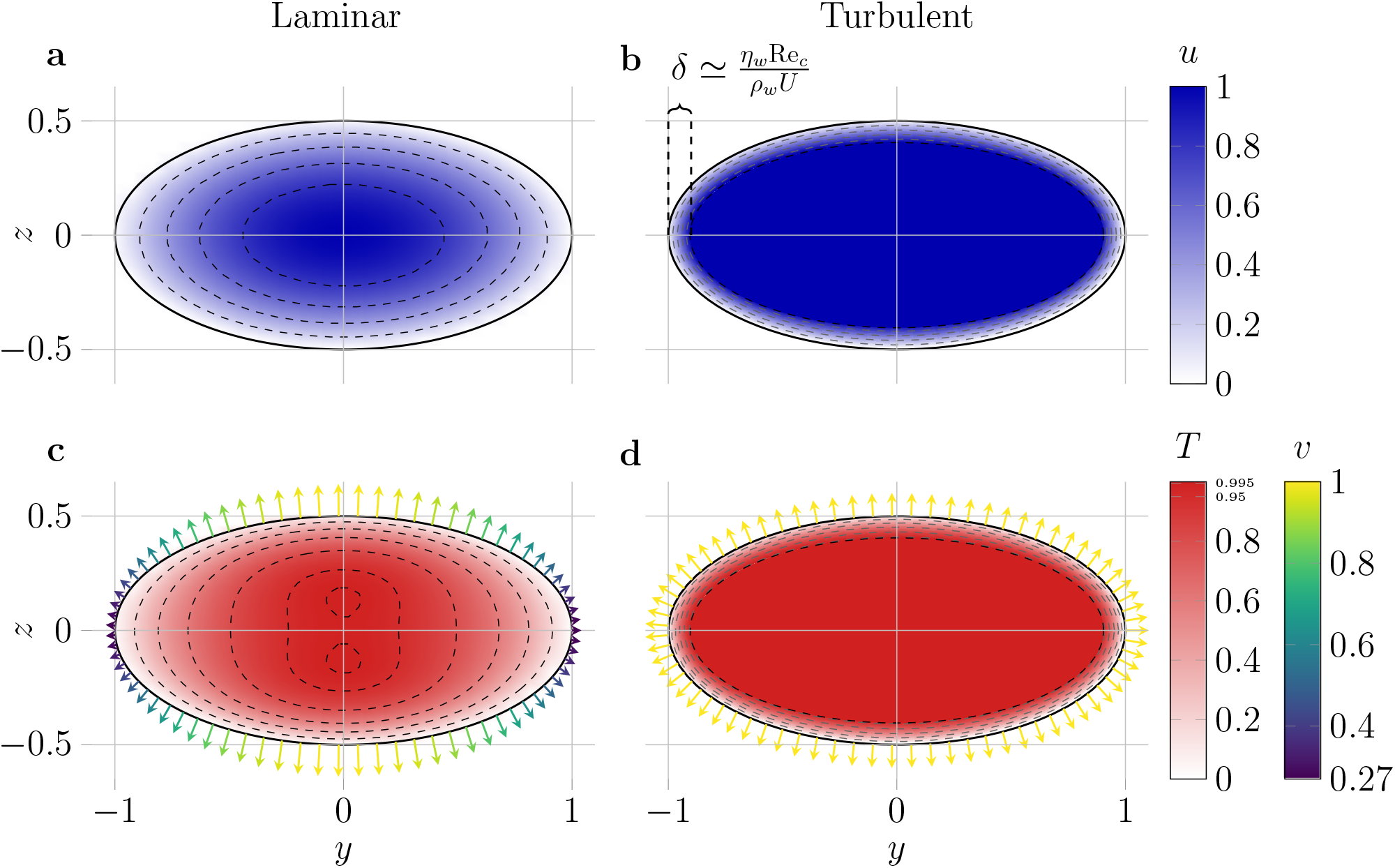


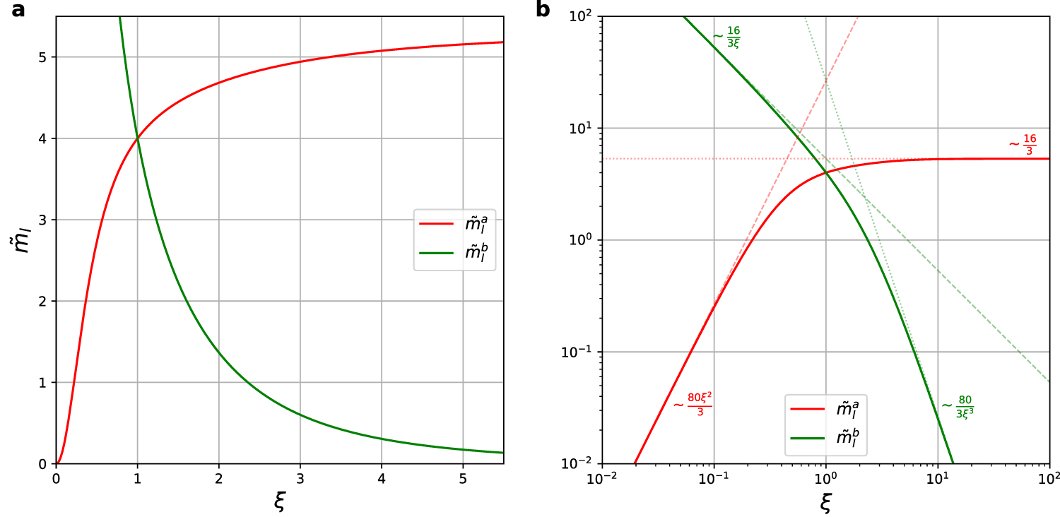


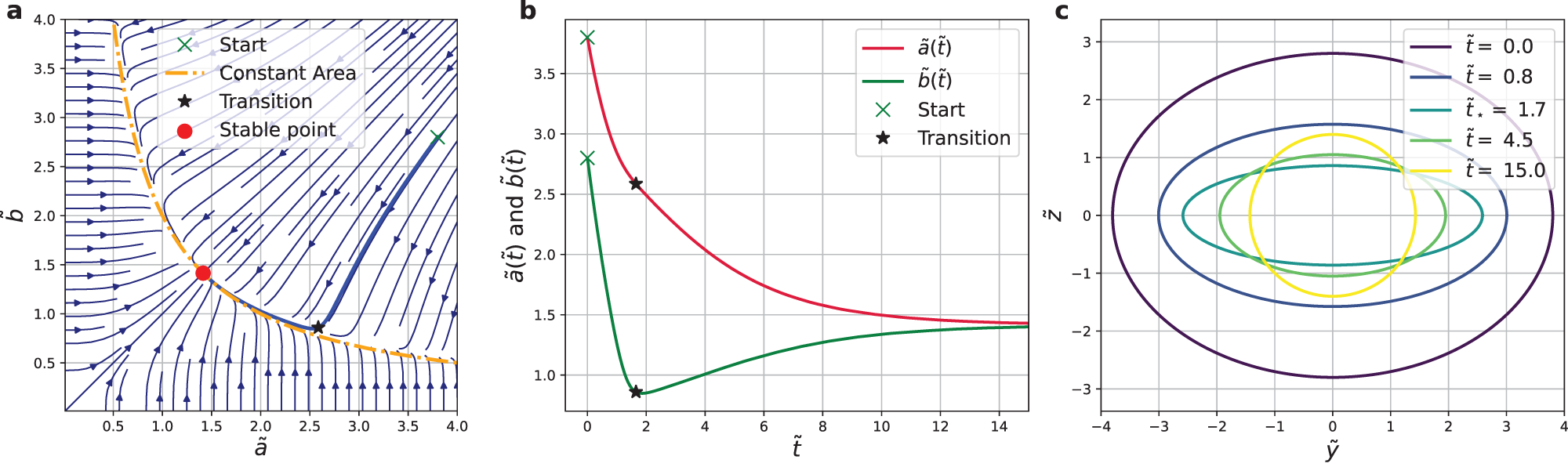
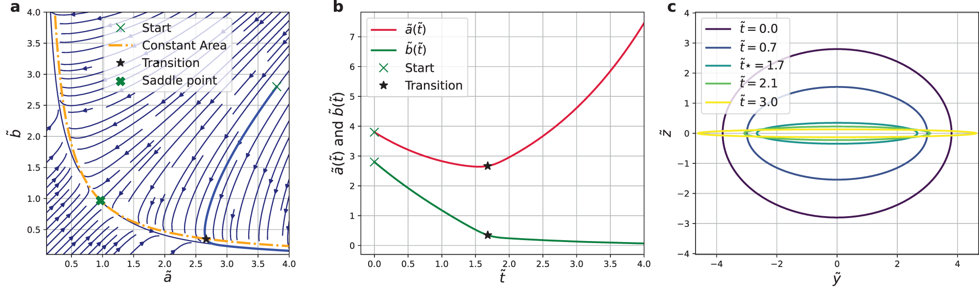
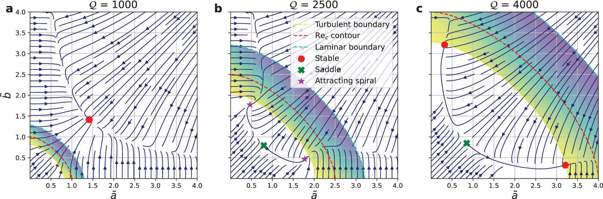


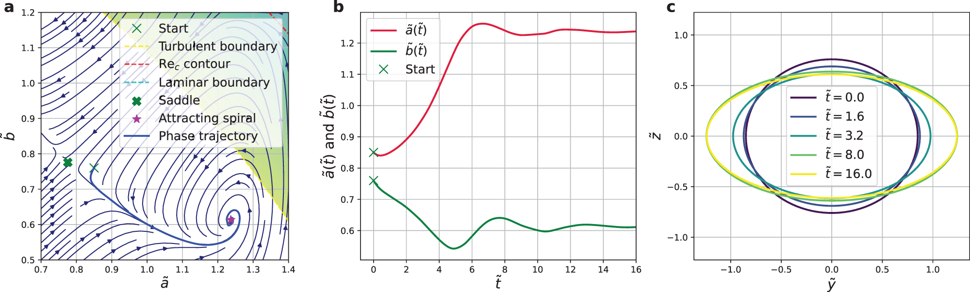


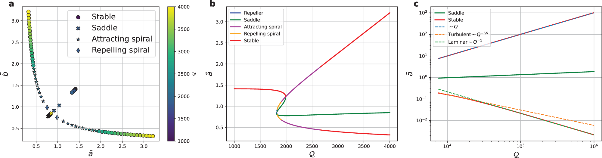


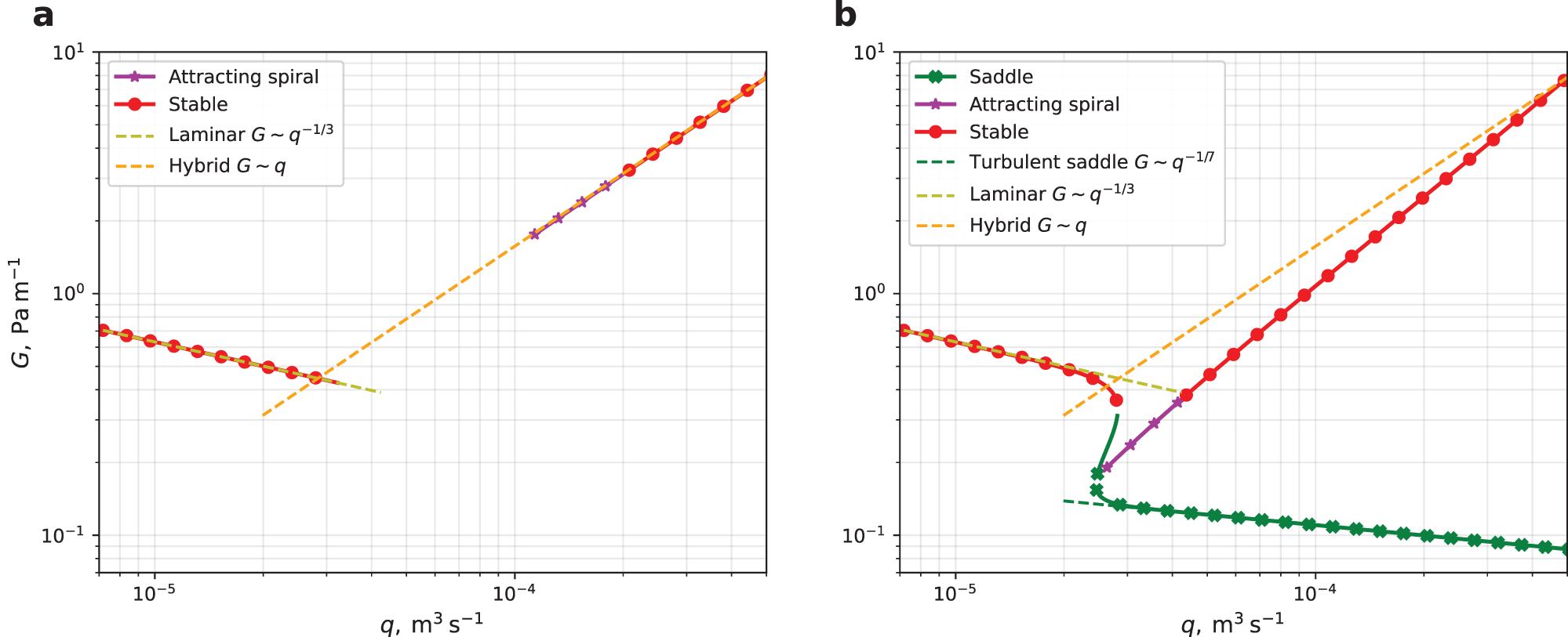


 Open access

