INTRODUCTION
The structure of ecological communities is thought to respond to interrelated factors acting at different spatial scales. Climate, historical processes and geology interact to determine plant community composition at the regional scale, whereas microclimate, edaphic conditions and species interactions play a major role in structuring plant communities at the local scale (Ricklefs Reference RICKLEFS1987, Reference RICKLEFS2004; Ricklefs & Schluter Reference RICKLEFS and SCHLUTER1993). Particularly interesting are studies that link explanatory variables obtained at one or more spatial scales with one or several aspects of species diversity (Ohmann & Spies Reference OHMANN and SPIES1998, Oliveira-Filho & Fontes Reference OLIVEIRA-FILHO and FONTES2000, Svenning & Skov Reference SVENNING and SKOV2005, Tuomisto et al. Reference TUOMISTO, POULSEN, RUOKOLAINEN, MORAN, QUINTANA, CELI and CAÑAS2003).
The importance of many factors in determining species composition and distribution may vary greatly with scale and locality (Condit et al. Reference CONDIT, PITMAN, LEIGH, CHAVE, TERBORGH, FOSTER, NUÑEZ VARGAS, AGUILAR, VALENCIA, VILLA MUÑOZ, MULLER-LANDAU, LOSOS and HUBBELL2002). In temperate forests, species turnover has been associated with environmental change at both landscape (Gilbert & Lechowicz Reference GILBERT and LECHOWICZ2004, Peterson & McCune Reference PETERSON and McCUNE2001) and regional scales (Lobo et al. Reference LOBO, CASTRO and MORENO2001, Ohmann & Spies Reference OHMANN and SPIES1998, Ricklefs et al. Reference RICKLEFS, QIAN and WHITE2004, Svenning & Skov Reference SVENNING and SKOV2005). In tropical forests, structure and diversity of plant communities have been associated mainly with soil conditions at a local scale (Clark et al. Reference CLARK, PALMER and CLARK1999, Phillips et al. Reference PHILLIPS, NÚÑEZ VARGAS, CHUSPE ZANS, GALIANO SÁNCHEZ, YLI-HALLA and ROSE2003, Tuomisto et al. Reference TUOMISTO, POULSEN, RUOKOLAINEN, MORAN, QUINTANA, CELI and CAÑAS2003) and climate at a regional scale (Duivenvoorden et al. Reference DUIVENVOORDEN, SVENNING and WRIGHT2002, Oliveira-Filho & Fontes Reference OLIVEIRA-FILHO and FONTES2000, Pyke et al. Reference PYKE, CONDIT, AGUILAR and LAO2001, Toledo et al. Reference TOLEDO, POOTER, PEÑA-CLAROS, ALARCON, BALCÁZAR, LEAÑO, LICONA, LLANQUE, VROOMANS, ZUIDEMA and BONGERS2010). In wet montane forests, vegetation dynamics and structure are heavily conditioned by climate, mediated by temperature and rainfall (Ashton Reference ASHTON2003, Bhattarai & Vetaas Reference BHATTARAI and VETAAS2003, Lieberman et al. Reference LIEBERMAN, LIEBERMAN, PERALTA and HARTSHORN1996, Vazquez & Givnish Reference VAZQUEZ and GIVNISH1998). Within a climatic region, vegetation is influenced by several other factors, including substrate, topography, soil composition (Ashton Reference ASHTON2003, Givnish Reference GIVNISH1999) and disturbance (Baruch Reference BARUCH1984, Martin et al. Reference MARTIN, SHERMAN and FAHEY2007).
Andean forests are particularly diverse and climatically and geomorphologically complex (Kappelle & Brown Reference KAPPELLE and BROWN2001). At the southernmost extension of Andean forests (southern Bolivia and north-western Argentina) and elsewhere (Gentry Reference GENTRY1988, Kessler Reference KESSLER2002), several studies have evaluated regional gradients in forest composition and structure (Brown & Ramadori Reference BROWN and RAMADORI1989, Brown et al. Reference BROWN, CHALUKIAN and MALMIERCA1985, Grau Reference GRAU2002, Grau et al. Reference GRAU, ARTURI, BROWN and ACEÑOLAZA1997, Morales et al. Reference MORALES, SIROMBRA, BROWN, Brown and Grau1995), but few have considered explicit links to potential explanatory factors (Aragón & Morales Reference ARAGÓN and MORALES2003, Lopez & Duque Reference LÓPEZ and DUQUE2010).
In this study, we assess the relative importance of local and regional environmental factors as determinants of changes in species composition across and within forests. Specifically, we studied: (1) the association of environmental factors with tree species composition along an Andean forest gradient; and (2) the relative importance of regional factors (i.e. climate), local factors (i.e. topography and disturbance) and spatial location for structuring tree communities at decreasing geographical extents from the complete gradient to specific forest types. We predict that climate (i.e. temperature and moisture) will best explain patterns of community composition at the regional scale. Then, as spatial extent decreases from the complete gradient to a particular forest type (i.e. dry and cloud forest), we predict that local factors will gain importance for explaining species composition. To evaluate these predictions, we undertook a quantitative analysis of tree species composition across 47 1-ha permanent plots within an area of about 25 000 km2 in north-western Argentina.
METHODS
Study area
Fieldwork was carried out in north-western Argentina within Andean forest (i.e. selva tucumano-boliviana; Cabrera Reference CABRERA1976) and its transition to chaco forest, which represent the southernmost extension of Neotropical montane forests located on the eastern Andean slope (Cabrera & Willink Reference CABRERA and WILLINK1980). Based on floristic composition, four vegetation units are differentiated along the altitudinal gradient; (1) chaco forest from c. 300–400 m asl; (2) lowland forest from c. 400–900 m asl; (3) lower montane forest from c. 900–1600 m asl; and (4) upper montane forest from c. 1600–2300 m asl (Cabrera Reference CABRERA1976). The tree flora of the area is relatively well known (Demaio et al. Reference DEMAIO, KARLIN and MEDINA2002, Digilio & Legname Reference DIGILIO and LEGNAME1966, Killeen et al. Reference KILLEEN, GARCIA and BECK1993, Legname Reference LEGNAME1982).
The study area covers a 250-km latitudinal transect from 22° S (border between Bolivia and Argentina) to 24° S (Salta and Jujuy Provinces, Argentina) and a 2000-m altitudinal gradient that can be divided into two main forest types: dry forest, from 300–400 m asl to c. 800–900 m asl; and cloud forest, from 800–900 m asl to tree line (c. 2300 m asl). Chaco and lowland forest are seasonally dry forests with >79% deciduous tree species (Sarmiento Reference SARMIENTO1972). Lower and upper montane forests are cloud forests with a high proportion of evergreen and semi-deciduous tree species (Brown et al. Reference BROWN, GRAU, MALIZIA, GRAU, Kappelle and Brown2001).
Climate is defined as subtropical with a marked dry season (April–October) and occasional frost during cold months (Brown et al. Reference BROWN, GRAU, MALIZIA, GRAU, Kappelle and Brown2001). Annual rainfall averages 625 mm (450–700 mm) in chaco forest, 820 mm (550–1400 mm) in lowland forest, 1800 mm (1100–2300 mm) in lower montane forests and 1100 mm (800–1400 mm) in upper montane forests (Bianchi & Yáñez Reference BIANCHI and YÁÑEZ1992). In cloud forests, water input through fog interception can equal direct rainfall (Hunzinger Reference HUNZINGER1997). Mean annual temperature is 21.5°C (mean maximum = 27.6°C, mean minimum = 15.4°C) in the lowlands and 11.7°C (mean maximum = 21.8°C, mean minimum = 8.8°C) in montane forest (Arias & Bianchi Reference ARIAS and BIANCHI1996).
Data collection
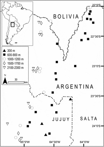
We established a network of 47 1-ha plots (45 permanent and two non-permanent plots) between 2003 and 2009, with plots distributed along the altitudinal gradient (Figure 1). All plots were established in relatively well-conserved forests (13 out of 47 plots were established in protected areas) undisturbed by human activities; e.g. selective logging, cattle transhumance. These activities have been practiced in the study area for at least the past 100 y (Brown et al. Reference BROWN, GRAU, MALIZIA, GRAU, Kappelle and Brown2001). For this reason, we included disturbance indicators such as cattle presence and stumps. Three plots were established in chaco forest (CF), 20 plots in lowland forest (LF), 10 plots in lower montane forest (1000–1200 m, LMF), seven plots in the transition between lower and upper montane forests (1500–1700 m, L-UMF), and seven plots in upper montane forest (2000–2300 m, UMF). In summary, 23 plots were established in dry forests and 24 plots in cloud forests.
Extent of study area and spatial location of 47 1-ha plots in Andean forests of north-western Argentina. Black symbols correspond to plots in dry forest and white symbols correspond to plots in cloud forest. Symbols indicate approximate plot elevation.

All plots were 20 × 500 m corrected for slope to cover 1 ha (Condit Reference CONDIT1998); orientation with respect to the main slope was random. A full inventory was made of all trees ≥10 cm dbh in every plot. Trees were marked with numbered aluminium tags, measured for dbh (1.30 m, avoiding trunk irregularities) and identified to species or morphospecies if field identification was not possible. We collected voucher specimens of all species and morphospecies sampled in the plots. Voucher specimens were distributed to taxonomic specialists or matched to specialist-identified material. One hundred individuals (0.4% of total) remained unidentified (e.g. trees with no leaves, database errors) and were excluded from all analyses.
Response and explanatory variables
Our response variable was number of individuals per species. Twenty-two species (involving only 41 individuals) were eliminated from the species data matrix because their poor representation introduced a large number of zeroes in the data matrix (Borcard et al. Reference BORCARD, LEGENDRE and DRAPEAU1992) and to avoid an unduly large influence on the analysis (ter Braak & Šmilauer Reference TER BRAAK and ŠMILAUER2002). The remaining 139 species (22 099 individuals) were included in the analyses.
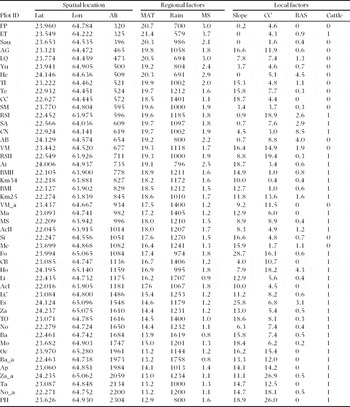
We compiled data on 10 explanatory variables pertaining to three subsets: spatial location, regional environmental factors and local environmental factors in each 1-ha plot (Appendix 1). We used a GPS unit to measure altitude at the extremes of each plot and used the average. We recorded latitude and longitude at the beginning of each plot. To account for complex non-linear spatial trends in species composition, we considered quadratic and cubic combinations of latitude and longitude (Borcard et al. Reference BORCARD, LEGENDRE and DRAPEAU1992). These derived spatial variables did not explain more species variation than raw latitude and longitude in a forward stepwise procedure and, therefore, only raw latitude and longitude measures were used in subsequent analyses. Altitude, latitude and longitude were considered as spatial variables.
We considered regional factors as those that can potentially vary across plots; i.e. climate. We derived climatic data from a local precipitation model and local mean monthly temperature from a map surface (http://www.inta.gov.ar/prorenoa/info/clima) developed by Bianchi et al. (Reference BIANCHI, ELENA and VOLANTE2008) for north-western Argentina. Both models were generated from 450 stations with weather data from 1934 to 1990. We used total annual rainfall and mean annual temperature as climatic variables. We log-transformed precipitation, following Ohmann & Spies (Reference OHMANN and SPIES1998), because vegetation does not respond linearly to precipitation; i.e. a 1-cm difference in precipitation is more important at low than at high levels. In addition, we included a derived climate index, moisture stress (MS,°C mm−1), which is a ratio between temperature and rainfall. Pronounced MS reflects higher temperatures coupled with lower rainfall.
We measured slope, per cent canopy cover (with a densitometer) and stump diameter in 25 quadrats of 20 × 20 m inside each plot. We considered these variables as local factors because they can potentially vary within each 1-ha plot. We used mean slope as a measure of topographic variation between plots, and canopy cover coefficient of variation and stump basal area as disturbance indicators. Additionally, we considered cattle presence-absence in each 1-ha plot from direct and indirect evidence (Appendix 1).
Data analyses
We analysed the entire dataset (47 1-ha plots) and each forest type separately (i.e. dry and cloud forests). Although the two forest subsets were not independent of the complete gradient, we analysed them separately because we wanted to stratify the gradient to examine within forest-type ecological variation and effects of geographic extent on ecological patterns.
To select the appropriate ordination techniques, species matrices for the entire gradient (47 plots, 139 species), dry forest (23 plots, 99 species) and cloud forest (24 plots, 113 species) were analysed using Detrended Correspondence Analysis (DCA; ter Braak Reference TER BRAAK and Bock1988), with detrending by segments and untransformed species data. Since the length of the extracted gradient was more than 4.0 SD units in all data-sets, we subsequently conducted Canonical Correspondence Analysis (CCA; Lepš & Šmilauer Reference LEPŠ and ŠMILAUER2003).
We performed CCAs with all explanatory variables to determine relationships between species and explanatory variables (H0: There are no relationships between species and explanatory variables matrices). We logarithmically transformed species relative abundance (i.e. log(x+1)) to dampen the influence of dominant species (Lepš & Šmilauer Reference LEPŠ and ŠMILAUER2003) and we down-weighted the influence of rare species (option available in CANOCO). We used Hill's scaling method on inter-sample distances, appropriate for data with large species turnover across samples. The fraction of species variation explained by the explanatory variables (total variation explained, TVE) was calculated as the sum of all canonical eigenvalues (or trace) divided by the total variation (TV) in the species data (total inertia sensu ter Braak & Šmilauer Reference TER BRAAK and ŠMILAUER2002). A Monte Carlo permutation test was performed to determine the accuracy of the relationship (999 randomizations) between species and explanatory variables. The trace was used to build the F-ratio statistic (ter Braak Reference TER BRAAK1990) and, when P < 0.05, the relationship between the two data-sets was considered significant. Then, a forward stepwise procedure was carried out to retain only significant variables for each set of explanatory data (i.e. spatial location, regional environmental factors and local environmental factors). We added explanatory variables in order of greatest additional contribution to TVE but only if they were significant (P < 0.05), where significance was determined by a Monte Carlo permutation test with 999 randomizations (H0: Additional influence of variables on vegetation is not significantly different from random), and if adding the variable did not cause any variance inflation factors (VIF) to exceed 3 (following Zuur et al. Reference ZUUR, IENO and ELPHICK2010). Variables with large inflation factors are strongly multicollinear with others and contribute little unique information to the model (Lepš & Šmilauer Reference LEPŠ and ŠMILAUER2003). We performed all analyses using CANOCO 4.5.
Variance partitioning with CCA was performed to evaluate the relative importance of spatial location, regional factors and local factors. First, we found the pure fraction of variation explained by each set of explanatory variables; i.e. the independent effects of space (S), regional environmental factors (R) and local environmental factors (L), using a set of variables as constraining variables and the others two sets as covariables (i.e. S|R+L, R|L+S, and L|R+S). Then, we found the mixed fractions of variation explained by all possible combinations of each sets of explanatory variables (i.e. R+S, L+S, R+L and R+L+S), following recommendations of Anderson & Gribble (Reference ANDERSON and GRIBBLE1998).
RESULTS
We marked and measured a total of 22 240 trees and 204 stumps in the 47 1-ha plots. We recorded 160 species (including three morphospecies), 124 genera and 60 families (Appendix 2). All species datasets exhibited large compositional gradients as estimated using DCA. Lengths of the extracted gradients in species-turnover SD units were: 7.4 and 4.0 for the complete gradient; 4.7 and 3.0 for dry forest; and 5.7 and 2.6 for cloud forest, for axes 1 and 2, respectively.
Environmental and spatial factors along an Andean forest gradient
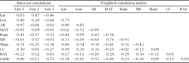
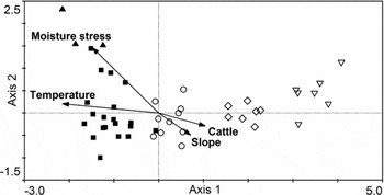
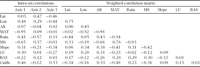
Considering the complete gradient, species composition and all explanatory variables were significantly correlated, as indicated by CCA with Monte Carlo permutation tests (P < 0.001 for the sum of all canonical axes). Species turnover was relatively high along the altitudinal gradient (eigenvalues 0.69, 0.28 and 0.14 for axes 1–3, respectively). The first canonical axis in the species ordination was correlated with altitude and temperature, followed by moisture stress (Table 1). Altitude was negatively correlated with temperature and moisture stress, indicating that the data structure summarized by the first axis primarily reflected a geographic gradient from a warmer and drier climate in the lowlands to a colder and wetter climate in the highlands (Figure 2).
Results of canonical correspondence analysis (CCA) for 47 1-ha plots in Andean forests of north-western Argentina considering 10 explanatory variables (spatial location, regional and local environmental factors). Intra-set correlations for the first three axes and weighted correlation matrix for the explanatory variables are shown. Latitude (Lat, °), longitude (Lon, °), altitude (Alt, m asl), mean annual temperature (MAT, °C), total annual rainfall (Rain, mm), moisture stress (MS, °C mm−1), mean slope (°), canopy cover coefficient of variation (CC), basal area of stumps (BAS, m2 ha−1) and cattle (presence = 1, absence = 0).
Biplot of sample plots and significant environmental variables from stepwise CCA for the altitudinal gradient in Andean forests of north-western Argentina. Symbols indicate approximate plot altitude: (▲) c. 300 m, (■) c. 600–900 m, (○) c. 1000–1200 m, (◇) c. 1500–1700 m, (▽) c. 2100–2300 m.

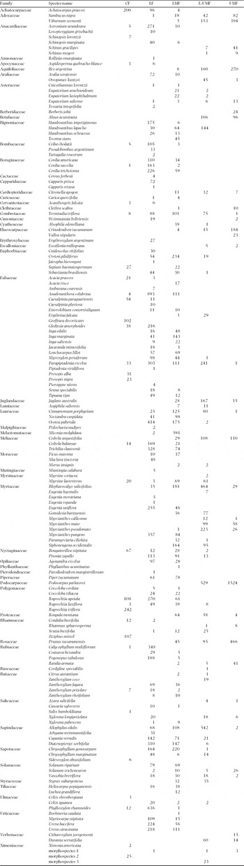
Plots with the lowest scores on axis 1 were located at lower altitudes and experienced higher temperatures and more pronounced moisture stress. These plots were located in CF and LF (dry forests). Species such as Achatocarpus praecox and Ruprechtia triflora were the most abundant in CF, whereas Anadenanthera colubrina, Phyllostylon rhamnoides and Ocotea puberula were the most abundant in LF (Appendix 2). Plots with intermediate scores were mainly located at 1000–1200 m in LMF and were characterized by steeper slopes. Miconia molibdaea, Croton piluliferus and Chrysophyllum gonocarpum were the most abundant tree species in LMF. Finally, plots with highest scores were located roughly above 1500 m and corresponded to L-UMF and UMF. These plots were characterized by low temperatures and presence of cattle (Figure 2). The most common tree species at this altitude were Podocarpus parlatorei, Viburnum seemenii and Blepharocalyx salicifolius (Appendix 2).
The second CCA axis partially showed a gradient of humidity from drier to wetter forests (highest to lowest scores on axis 2). The compositional gradient reflected by the second axis was negatively correlated with rainfall and positively correlated with moisture stress (Table 1). When a stepwise procedure was performed, only moisture stress was included in the simple model to avoid collinearity, because this variable explained a higher proportion of total variation. Finally, the third CCA axis (not shown) tended to segregate plots within altitudes (mainly at LF and LMF), based on cattle presence and slope (Table 1).
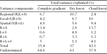
Simpler models, with all significant environmental (regional and local) and spatial variables obtained by stepwise forward selection, explained 35.4% of the variation in tree-species composition and abundance along the complete gradient. Spatial factors (altitude and latitude) explained 4.8% of total variation (TV), regional factors (temperature and moisture stress) explained 6.7% of TV, and local factors (slope and cattle presence) explained 4.2% of TV. Regional environmental factors spatially structured (R+S) explained 13.4% of TV and environmental (both regional and local) factors spatially structured (R+L+S) explained 5% of TV. Based on these results, altitude was correlated with temperature and moisture stress (regional factors) and with cattle presence (local factors; Table 1) and accounted for a large proportion of the spatial structure in environmental variation.
Relative importance of regional, local and spatial factors within forest types
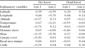
Species composition and all explanatory variables were significantly correlated within dry forest (P < 0.004) and within cloud forest (P < 0.002), as indicated by CCA results with Monte Carlo permutation tests. Dry forest showed more than one environmental gradient, as reflected by percentage of variation explained by axes 1 and 2 (eigenvalues 0.36, 0.23 and 0.18 for axes 1–3, respectively). The first canonical axis in species ordination was correlated with moisture stress, rainfall and temperature but only moisture stress was included in the simple model in stepwise procedure. The second canonical axis was correlated with longitude and cattle presence (Table 2). Cloud forest showed a main environmental gradient along axis 1 (eigenvalues 0.64, 0.22 and 0.17 for axes 1–3, respectively). The first canonical axis in the species ordination was correlated with altitude and temperature, reflecting the spatial structure in regional factors. The second canonical axis was correlated with stump basal area and cattle presence (Table 2).
Results of canonical correspondence analyses (CCAs) for 23 1-ha plots in dry forest and 24 1-ha plots in cloud forest in Andean forests of north-western Argentina. Intra-set correlations for the first two axes in CCAs with 10 explanatory variables (spatial location, regional and local environmental factors) are shown.

Variance partitioning results varied between dry and cloud forests (Table 3). Reduced models with all significant environmental (regional and local) and spatial variables explained 37% and 42.1% of TV in tree-species composition in dry and cloud forests, respectively. Considered separately, spatial factors explained more TV in cloud forest, whereas climate explained more TV in dry forest. Local factors alone explained about 10% of TV in both forest types. In dry forest, local environmental factors spatially structured (L+S) explained 4.8% of TV. In cloud forest, regional environmental factors spatially structured (R+S) explained 13.7% of TV and environmental (both regional and local) factors spatially structured (R+L+S) explained 4.1% of TV, similar to the results observed at the complete gradient.
Variance decomposition by partial CCA (following Anderson & Gribble Reference ANDERSON and GRIBBLE1998) of species abundance data into pure regional (R not shared with L and S), pure local (L not shared with R and S), pure spatial (S not shared with R and L), and all possible mixed components for all datasets. R = regional variables, L = local variables and S = spatial variables.

DISCUSSION
This study is the first systematic quantification of tree-community composition and abundance and its association with environmental variables for subtropical Andean forest at the regional scale. Our modest performance in explaining variation in tree species composition (~35%) is common in floristic gradient analyses, where some overlooked factors or large amounts of stochastic variation remain unclear (Borcard et al. Reference BORCARD, LEGENDRE and DRAPEAU1992). Still, low explained variances do not impair the significance of species-environmental relations (ter Braak Reference TER BRAAK and Bock1988).
The issue of scale in defining the relative importance of explanatory variables in ecological communities has received increased recognition in recent decades (Ashton Reference ASHTON2003, Ricklefs Reference RICKLEFS2004). In regional studies of plant distribution or diversity, a primary control of regional factors over local factors is common, but the identity of the main factors usually changes among studies (e.g. climate: Ohmann & Spies Reference OHMANN and SPIES1998; geology and spatial variables: Lobo et al. Reference LOBO, CASTRO and MORENO2001; history: Svenning & Skov Reference SVENNING and SKOV2005). In our study, the relative contribution of the explanatory variables was influenced by geographic extent and location (i.e. from the complete gradient to within forest type), and varied with the scale of the explanatory factor (i.e. regional vs. local environmental factors).
Factors influencing tree species distribution along an Andean forest gradient
Tree community composition along the Andean forest gradient was predominantly controlled by regional environmental factors that were spatially structured (i.e. R+S explained 13% TV). The altitudinal gradient varied from a warm and dry climate in the lowlands to a cold and wet climate higher in the mountains. The strong spatial structure of the climatic variables is partially due to spatial autocorrelation (Borcard et al. Reference BORCARD, LEGENDRE and DRAPEAU1992), since altitude and temperature were highly correlated. We found a strong association between altitude and species composition, as observed in other vegetation studies (Bhattarai & Vetaas Reference BHATTARAI and VETAAS2003, Carpenter Reference CARPENTER2005, Ohmann & Spies Reference OHMANN and SPIES1998, Vazquez & Givnish Reference VAZQUEZ and GIVNISH1998). In our study, altitude explained more variation in species composition than any other variable both along the complete gradient and within cloud forest. In contrast to temperature, precipitation is commonly found to have a relatively complex pattern (Lomolino Reference LOMOLINO2001), statistically independent of a linear change in altitude. Rainfall in subtropical Andean forest has a unimodal trend, which peaks at LMF (1000–1200 m asl). Therefore, altitude is a complex gradient where several biotic and abiotic factors correlate (Grubb Reference GRUBB1977, Kitayama Reference KITAYAMA1992, Whittaker Reference WHITTAKER1967). The interaction between a variable with a linear response (temperature) and a variable with a unimodal response (rainfall) may partially explain the patterns in species composition reported here.
After removing the spatial structure from the species composition data, the fraction explained by regional factors alone (R|L+S) was higher than the fraction explained by local factors (L|R+S). Our results support the prediction that climate is the primary control of community composition along the complete altitudinal gradient. Brown et al. (Reference BROWN, GRAU, MALIZIA, GRAU, Kappelle and Brown2001) suggest that climatic variables play an important role in determining tree-species distribution across and within Andean forest. Our findings support the conceptual model of multi-scale controls on vegetation distribution, where local community structure results from a combination of both regional and local-scale processes (Ricklefs Reference RICKLEFS2004).
Relative importance of regional and local environmental factors within forest types
Species composition was structured by two main sets of variables within dry forest, where independent effects of local and regional factors contributed in quite similar proportions (~9–10% each). We predicted that local environmental factors would increase their relative importance in explaining species composition as geographic extent of analysis decreased from the complete gradient to a particular forest type. Although the relative importance of local environmental factors increased within dry forest, we found that climate also explained a high proportion of variation in community composition. Moisture stress best explained tree-species composition, followed by cattle presence and slope. Elevated levels of moisture stress reflect high temperatures coupled with low rainfall. These extreme conditions occur prior to the beginning of the wet season, when temperatures may reach 40°C (October–November). Additionally, there is a decreasing rainfall gradient within dry forest of about 150 mm of total annual rainfall from the north-eastern side towards the south-western side of the study area (Appendix 1), which produces dramatic changes in species abundance. For example, Diatenopteryx sorbifolia, Ocotea puberula, Cordia americana and Eugenia uniflora showed the highest relative abundance on the more humid north-eastern side, but were poorly represented on the south-western side. Similarly, Calycophyllum multiflorum, Phyllostylon rhamnoides, Astronium urundeuva and Anadenanthera colubrina were the most abundant species on the south-western side, but showed low relative abundance on the north-eastern side.
The pattern within cloud forest was similar to that for the complete gradient; i.e. altitude and temperature best explained variation in tree-species composition. Low temperatures are well known to affect tree distribution and diversity towards the tree line (Givnish Reference GIVNISH1999, Stevens & Fox Reference STEVENS and FOX1991) by allowing only a subset of high-montane forest trees to reach high altitudes (39 out of 160 species sampled were present at c. 2100 m). After removing the spatial structure from the species composition data, the fraction explained only by regional factors was lower than the fraction explained by local factors alone (2.4% and 9.4%, respectively). This result supports our second prediction, stating that when the spatial scale of analysis is reduced from the complete gradient to a particular forest type (i.e. cloud forest), local environmental factors would increase in relative importance.
A disturbance gradient, mainly represented by cattle presence, also explained a high proportion of variation in species composition in Andean forests at both geographic extents (the complete gradient and within forest types). Baruch (Reference BARUCH1984) has reported that vegetation changes along an altitudinal gradient in Venezuela appear to be related primarily to environmental changes occurring with altitude, and secondarily to disturbances caused mainly by grazing. Livestock is a long-standing disturbance factor in Andean forest of north-western Argentina. Local people have been practising cattle transhumance for centuries, alternating grazing at grasslands above the tree-line during the warm season with grazing within the forest during the cold season (Ramadori & Brown Reference RAMADORI, BROWN, Lieberman and Baied1997). Effects of livestock transhumance on seedling establishment and mortality of Cedrela angustifolia (a timber tree species) were reported for Andean forest in southern Bolivia (Zamora Petri Reference ZAMORA PETRI, Pacheco and Brown2006). However, no studies have evaluated the effect of cattle on species composition and forest structure at the community level. Whereas livestock is an historical anthropogenic disturbance in Andean forest (Brown et al. Reference BROWN, GRAU, MALIZIA, GRAU, Kappelle and Brown2001, Reboratti Reference REBORATTI, Brown and Grau1995), this practice could influence species composition by promoting different environmental conditions for tree establishment and growth. Finally, our results support the notion that where regional climate is more stressful for plant life (e.g. dry and hot in lowlands and cold in mountains), species respond to smaller-scale variation in local factors such as topography, soil conditions and biotic interactions (Neilson et al. Reference NEILSON, KING, DEVELICE, LENIHAN, Hansen and di Castri1992).
In this study, we found that a small set of explanatory variables account for about 35–40% of the variation in tree-species composition and abundance in the spatially and environmentally heterogeneous Andean forests of north-western Argentina. Considerations of smaller spatial extent (e.g. local scale) and plots (e.g. 0.1 ha) might have increased the match between species composition and local factors, enhancing in turn the relative importance of local factors and the total amount of floristic variation explained. It seems clear from this study, however, that consideration of both local and regional environmental factors may be a useful approach to understand tree community composition and variation across and within forests.
ACKNOWLEDGEMENTS
C. Aguirre, E. Toranzo, M. J. Tulli, E. Cuyckens, W. Villafañe, U. Colina, G. Quintana, R. Guevara, E. Abán, A. Tauro, D. Delgado and A. Piggot provided field assistance. K. Buzza, S. Pacheco and L. Cristobal provided laboratory assistance. We thank the US National Science Foundation, Whitney R. Harris World Ecology Center (formerly International Center for Tropical Ecology) at the University of Missouri-St. Louis, Fundación ProYungas (Argentina) and Idea Wild for financial support. We thank the authorities of Secretaría de Gestión Ambiental (Provincia de Jujuy), Secretaría de Medio Ambiente y Desarrollo Sustentable (Provincia de Salta) and Administración de Parques Nacionales for work permission, and many private owners for allowing us to work on their properties.
Summary of 10 explanatory variables by subset (spatial, regional environmental factors and local environmental variables) for 47 1-ha plots along the altitudinal gradient in Andean forests of north-western Argentina. Latitude (Lat, °), longitude (Lon, °), altitude (Alt, m asl), mean annual temperature (MAT, °C), total annual rainfall (Rain, mm), moisture stress (MS, °C mm−1), mean slope (°), canopy cover coefficient of variation (CC), basal area stumps (BAS, m2 ha−1) and cattle (presence = 1, absence = 0).

Species and absolute abundance recorded in 47 1-ha plots along the altitudinal gradient in Andean forests of north-western Argentina. Chaco forest (CF), lowland forest (LF), lower montane forest (LMF), transition between lower and upper montane forests (L-UMF), and upper montane forest (UMF). Nomenclature follows http://www2.darwin.edu.ar/Proyectos/FloraArgentina/FA.asp.