2.1 The generalised scale-by-scale energy budget

The most general forms of the scale-by-scale energy budget for incompressible turbulent flows have been derived without making any assumption about the nature of the turbulence by Duchon & Robert (Reference Duchon and Robert1999) without averaging and by Hill (Reference Hill1997, Reference Hill2001, Reference Hill2002a ) with averaging. Using the Reynolds decomposition (capital letters and $\langle \cdots \rangle$ indicate ensemble- and/or time-averaged quantities), the equation derived by Hill (Reference Hill1997, Reference Hill2001, Reference Hill2002a ) (which we refer to as the KHMH equation) takes the form (see also Danaila et al. Reference Danaila, Krawczynski, Thiesset and Renou2012)

where $\unicode[STIX]{x1D6FF}q^{2}=\unicode[STIX]{x1D6FF}u_{i}\unicode[STIX]{x1D6FF}u_{i}$ in terms of the fluctuating velocity differences $\unicode[STIX]{x1D6FF}u_{i}=u_{i}^{+}-u_{i}^{-}$ (for components $i=1,2,3$ ), $\unicode[STIX]{x1D6FF}U_{i}=U_{i}^{+}-U_{i}^{-}$ , where $U_{i}$ is a mean flow velocity component, $\unicode[STIX]{x1D6FF}p=p^{+}-p^{-}$ , where $p$ is fluctuating pressure, and the superscripts $+$ and $-$ distinguish quantities evaluated at $x_{i}+r_{i}/2$ and $x_{i}-r_{i}/2$ 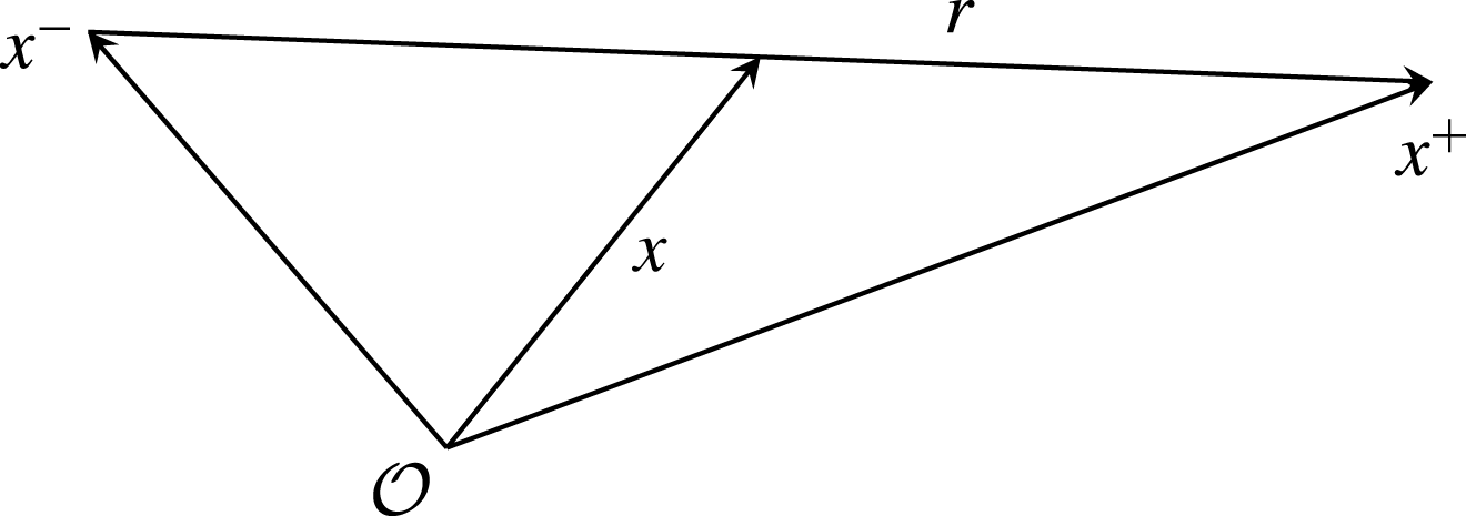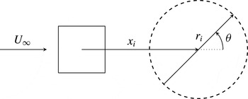respectively, as illustrated in figure 1. Equation (2.1) is written in a six-dimensional reference frame $x_{i},r_{i}$ , where coordinates $x_{i}$ are associated with a location in physical space, and the scale space is the space of all separations and orientations $\boldsymbol{r}=(r_{1},r_{2},r_{3})$ between two points (we refer to $r=|\boldsymbol{r}|$ as a scale). Throughout this paper, in the context of two-point statistics, we refer to isotropy as the independence of a given quantity from the orientation of the separation vector  $\boldsymbol{r}$ .

Figure 1.

Illustration of the spatial position vectors $\boldsymbol{x}=(x_{1},x_{2},x_{3})$ , $\boldsymbol{x}^{+}=(x_{1}^{+},x_{2}^{+},x_{3}^{+})$ and $\boldsymbol{x}^{-}=(x_{1}^{-},x_{2}^{-},x_{3}^{-})$ in a reference frame centred on ${\mathcal{O}}$ , and of the separation vector $\boldsymbol{r}=(r_{1},r_{2},r_{3})$ .

We follow Gomes-Fernandes et al. (Reference Gomes-Fernandes, Ganapathisubramani and Vassilicos2015) and Valente & Vassilicos (Reference Valente and Vassilicos2015) in the way that we identify the terms in (2.1) as

where each term is associated with a physical process in the budget of $\langle \unicode[STIX]{x1D6FF}q^{2}\rangle$ .

1. (i) The term $4{\mathcal{A}}_{t}=(\unicode[STIX]{x2202}\langle \unicode[STIX]{x1D6FF}q^{2}\rangle )/\unicode[STIX]{x2202}t$ represents the rate of change in time of $\langle \unicode[STIX]{x1D6FF}q^{2}\rangle$ at a given physical point $x_{i}$ and separation $r_{i}$ . In the present paper, statistics are collected in time (as opposed to ensemble averages) and therefore ${\mathcal{A}}_{t}$ vanishes.

2. (ii) The term $4{\mathcal{A}}=(\unicode[STIX]{x2202}((U_{i}^{+}+U_{i}^{-})/2)\langle \unicode[STIX]{x1D6FF}q^{2}\rangle )/\unicode[STIX]{x2202}x_{i}$ is the advection term. This term represents the transport of $\langle \unicode[STIX]{x1D6FF}q^{2}\rangle$ in physical space $x_{i}$ by the mean flow. In fact, integration of ${\mathcal{A}}$ over a volume ${\mathcal{V}}_{x}$ in physical space and use of Gauss’ theorem yields $\iiint _{{\mathcal{V}}_{x}}{\mathcal{A}}\,\text{d}V=\unicode[STIX]{x0222F}_{\unicode[STIX]{x2202}{\mathcal{V}}_{x}}((U_{i}^{+}+U_{i}^{-})/2)\langle \unicode[STIX]{x1D6FF}q^{2}\rangle n_{i}\,\text{d}S$ , which is the integral of a flux through $\unicode[STIX]{x2202}{\mathcal{V}}_{x}$ , the boundary of ${\mathcal{V}}_{x}$ . If this volume encompasses a set of mean streamlines, the flux integral is proportional to the difference of $\langle \unicode[STIX]{x1D6FF}q^{2}\rangle$ between the downstream and upstream boundaries in the case of homogeneous turbulence, in which case ${\mathcal{A}}$ accounts for the decay of $\langle \unicode[STIX]{x1D6FF}q^{2}\rangle$ in the direction of the mean flow (Hill Reference Hill2002b ; Thiesset et al. Reference Thiesset, Antonia and Danaila2013a ).

3. (iii) The term $4\unicode[STIX]{x1D6F1}=(\unicode[STIX]{x2202}\langle \unicode[STIX]{x1D6FF}u_{i}\unicode[STIX]{x1D6FF}q^{2}\rangle )/\unicode[STIX]{x2202}r_{i}$ is the nonlinear interscale transfer rate and accounts for the effect of nonlinear interactions in redistributing $\unicode[STIX]{x1D6FF}q^{2}$ within the $r_{i}$ space, and is given by the divergence in scale space of the flux $\langle \unicode[STIX]{x1D6FF}u_{i}\unicode[STIX]{x1D6FF}q^{2}\rangle$ . If one takes the integral of $\unicode[STIX]{x1D6F1}$ over a volume in scale space ${\mathcal{V}}_{r}$ , then, similarly to the discussion above, one obtains the flux integral $\unicode[STIX]{x0222F}_{\unicode[STIX]{x2202}{\mathcal{V}}_{r}}\langle \unicode[STIX]{x1D6FF}u_{i}\unicode[STIX]{x1D6FF}q^{2}\rangle n_{i}\,\text{d}S$ . If ${\mathcal{V}}_{r}$ is taken to be a sphere of radius $\ell$ , then $\iiint _{{\mathcal{V}}_{r}}\unicode[STIX]{x1D6F1}\,\text{d}V$ is proportional to the orientation-averaged flux $\langle \unicode[STIX]{x1D6FF}\boldsymbol{u}\unicode[STIX]{x1D6FF}q^{2}\rangle$ in scale space, corresponding to a length scale equal to the radius of the sphere.

4. (iv) The term $4\unicode[STIX]{x1D6F1}_{U}=(\unicode[STIX]{x2202}\unicode[STIX]{x1D6FF}U_{i}\langle \unicode[STIX]{x1D6FF}q^{2}\rangle )/\unicode[STIX]{x2202}r_{i}$ is the linear interscale transfer rate. Similarly to $\unicode[STIX]{x1D6F1}$ , this term accounts for transfer of $\unicode[STIX]{x1D6FF}q^{2}$ in scale space $r_{i}$ , but, instead of $\unicode[STIX]{x1D6FF}u_{i}$ , it is the two-point difference of mean velocity $\unicode[STIX]{x1D6FF}U_{i}$ that transports $\unicode[STIX]{x1D6FF}q^{2}$ in scale space.

5. (v) The term $4{\mathcal{P}}=-2\langle \unicode[STIX]{x1D6FF}u_{i}\unicode[STIX]{x1D6FF}u_{j}\rangle (\unicode[STIX]{x2202}\unicode[STIX]{x1D6FF}U_{j}/\unicode[STIX]{x2202}r_{i})-\langle (u_{i}^{+}+u_{i}^{-})\unicode[STIX]{x1D6FF}u_{j}\rangle (\unicode[STIX]{x2202}\unicode[STIX]{x1D6FF}U_{j}/\unicode[STIX]{x2202}x_{i})$ can be associated with the production of $\langle \unicode[STIX]{x1D6FF}q^{2}\rangle$ by mean flow gradients. Writing $4{\mathcal{P}}$ in terms of $x_{i}^{\pm }=x_{i}\pm r_{i}/2$ yields $-2\langle u_{i}^{+}u_{j}^{+}\rangle (\unicode[STIX]{x2202}U_{i}^{+}/\unicode[STIX]{x2202}x_{j}^{+})-2\langle u_{i}^{-}u_{j}^{-}\rangle (\unicode[STIX]{x2202}U_{i}^{-}/\unicode[STIX]{x2202}x_{j}^{-})+2\langle u_{i}^{-}u_{j}^{+}\rangle (\unicode[STIX]{x2202}U_{i}^{+}/\unicode[STIX]{x2202}x_{j}^{+})+2\langle u_{i}^{+}u_{j}^{-}\rangle (\unicode[STIX]{x2202}U_{i}^{-}/\unicode[STIX]{x2202}x_{j}^{-})$ , where the first two terms represent the production terms in the one-point turbulent kinetic energy equation and the last two represent combined actions of the mean flow gradients and the two-point correlation tensors $\langle u_{i}^{\pm }u_{j}^{\mp }\rangle$ (see, e.g., Lindborg Reference Lindborg1996, where such terms are related to the equation for $\langle \unicode[STIX]{x1D6FF}u_{i}\unicode[STIX]{x1D6FF}u_{j}\rangle$ ). Furthermore, if one writes the interscale energy budget for $\unicode[STIX]{x1D6FF}Q^{2}=\unicode[STIX]{x1D6FF}U_{i}\unicode[STIX]{x1D6FF}U_{i}$ , which is the mean flow equivalent to (2.1), the term ${\mathcal{P}}$ appears as it does in (2.1) but with the opposite sign,

   (2.3) $$\begin{eqnarray}\displaystyle & & \displaystyle \frac{\unicode[STIX]{x2202}\unicode[STIX]{x1D6FF}Q^{2}}{\unicode[STIX]{x2202}t}+\frac{\unicode[STIX]{x2202}{\displaystyle \frac{U_{i}^{+}+U_{i}^{-}}{2}}\unicode[STIX]{x1D6FF}Q^{2}}{\unicode[STIX]{x2202}x_{i}}+\frac{\unicode[STIX]{x2202}\langle \unicode[STIX]{x1D6FF}u_{i}\unicode[STIX]{x1D6FF}\boldsymbol{u}\boldsymbol{\cdot }\unicode[STIX]{x1D6FF}\boldsymbol{U}\rangle }{\unicode[STIX]{x2202}r_{i}}+\frac{\unicode[STIX]{x2202}\unicode[STIX]{x1D6FF}U_{i}\unicode[STIX]{x1D6FF}Q^{2}}{\unicode[STIX]{x2202}r_{i}}=2\langle \unicode[STIX]{x1D6FF}u_{i}\unicode[STIX]{x1D6FF}u_{j}\rangle \frac{\unicode[STIX]{x2202}\unicode[STIX]{x1D6FF}U_{j}}{\unicode[STIX]{x2202}r_{i}}\nonumber\\ \displaystyle & & \displaystyle \quad +\,\langle (u_{i}^{+}+u_{i}^{-})\unicode[STIX]{x1D6FF}u_{j}\rangle \frac{\unicode[STIX]{x2202}\unicode[STIX]{x1D6FF}U_{j}}{\unicode[STIX]{x2202}x_{i}}-\frac{\unicode[STIX]{x2202}\left\langle {\displaystyle \frac{u_{i}^{+}+u_{i}^{-}}{2}}\unicode[STIX]{x1D6FF}\boldsymbol{u}\boldsymbol{\cdot }\unicode[STIX]{x1D6FF}\boldsymbol{U}\right\rangle }{\unicode[STIX]{x2202}x_{i}}-2\frac{\unicode[STIX]{x2202}\langle \unicode[STIX]{x1D6FF}U_{i}\unicode[STIX]{x1D6FF}P\rangle }{\unicode[STIX]{x2202}x_{i}}+\unicode[STIX]{x1D708}\frac{1}{2}\frac{\unicode[STIX]{x2202}^{2}\unicode[STIX]{x1D6FF}Q^{2}}{\unicode[STIX]{x2202}x_{i}\unicode[STIX]{x2202}x_{i}}\nonumber\\ \displaystyle & & \displaystyle \quad +\,2\unicode[STIX]{x1D708}\frac{\unicode[STIX]{x2202}^{2}\unicode[STIX]{x1D6FF}Q^{2}}{\unicode[STIX]{x2202}r_{i}\unicode[STIX]{x2202}r_{i}}-4\unicode[STIX]{x1D708}\left(\left\langle \frac{\unicode[STIX]{x2202}\unicode[STIX]{x1D6FF}U_{j}}{\unicode[STIX]{x2202}x_{i}}\frac{\unicode[STIX]{x2202}\unicode[STIX]{x1D6FF}U_{j}}{\unicode[STIX]{x2202}x_{i}}\right\rangle +\frac{1}{4}\left\langle \frac{\unicode[STIX]{x2202}\unicode[STIX]{x1D6FF}U_{j}}{\unicode[STIX]{x2202}r_{i}}\frac{\unicode[STIX]{x2202}\unicode[STIX]{x1D6FF}U_{j}}{\unicode[STIX]{x2202}r_{i}}\right\rangle \right).\end{eqnarray}$$
   It follows that the interscale energy budget for $\langle [(U_{i}^{+}+u_{i}^{+})-(U_{i}^{-}+u_{i}^{-})][(U_{i}^{+}+u_{i}^{+})-(U_{i}^{-}+u_{i}^{-})]\rangle$ , which equals $\unicode[STIX]{x1D6FF}Q^{2}+\langle \unicode[STIX]{x1D6FF}q^{2}\rangle$ , does not involve ${\mathcal{P}}$ . This observation consolidates the interpretation of ${\mathcal{P}}$ as a production term. When ${\mathcal{P}}$ is positive/negative, energy is therefore lost/gained by $\unicode[STIX]{x1D6FF}Q^{2}$ and gained/lost by $\langle \unicode[STIX]{x1D6FF}q^{2}\rangle$ at the same rate. This process is only significant at large enough values of $r$ where $\unicode[STIX]{x1D6FF}Q^{2}$ is not negligible. It should be noted that $(\unicode[STIX]{x2202}\langle \unicode[STIX]{x1D6FF}u_{i}\unicode[STIX]{x1D6FF}\boldsymbol{u}\boldsymbol{\cdot }\unicode[STIX]{x1D6FF}\boldsymbol{U}\rangle )/\unicode[STIX]{x2202}r_{i}$ is the difference between the interscale energy transfer rate of the total two-point kinetic energy, $(\unicode[STIX]{x2202}\langle \unicode[STIX]{x1D6FF}u_{i}(1/2)(\unicode[STIX]{x1D6FF}\boldsymbol{U}+\unicode[STIX]{x1D6FF}\boldsymbol{u})^{2}\rangle )/\unicode[STIX]{x2202}r_{i}$ , and the interscale energy transfer rate, $2\unicode[STIX]{x1D6F1}=(\unicode[STIX]{x2202}\langle \unicode[STIX]{x1D6FF}u_{i}\unicode[STIX]{x1D6FF}q^{2}\rangle )/\unicode[STIX]{x2202}r_{i}$ of $\unicode[STIX]{x1D6FF}q^{2}/2$ . All of the other terms in (2.3) can be interpreted in the same way as their analogues in (2.1), except for the term $(\unicode[STIX]{x2202}\langle ((u_{i}^{+}+u_{i}^{-})/2)\unicode[STIX]{x1D6FF}\boldsymbol{u}\boldsymbol{\cdot }\unicode[STIX]{x1D6FF}\boldsymbol{U}\rangle )/\unicode[STIX]{x2202}x_{i}$ , which we discuss in (vi).

6. (vi) The term $4{\mathcal{T}}_{u}=-(\unicode[STIX]{x2202}\langle ((u_{i}^{+}+u_{i}^{-})/2)\unicode[STIX]{x1D6FF}q^{2}\rangle )/\unicode[STIX]{x2202}x_{i}$ is the transport of $\unicode[STIX]{x1D6FF}q^{2}$ in physical space due to turbulent fluctuations. It features in (2.1), whereas the term $(\unicode[STIX]{x2202}\langle ((u_{i}^{+}+u_{i}^{-})/2)\unicode[STIX]{x1D6FF}\boldsymbol{u}\boldsymbol{\cdot }\unicode[STIX]{x1D6FF}\boldsymbol{U}\rangle )/\unicode[STIX]{x2202}x_{i}$ , which features in (2.3), is the difference between the turbulent transport of total two-point kinetic energy $(\unicode[STIX]{x1D6FF}\boldsymbol{U}+\unicode[STIX]{x1D6FF}\boldsymbol{u})^{2}/2$ in physical space and $2{\mathcal{T}}_{u}$ .

7. (vii) The term $4{\mathcal{T}}_{p}=-2(\unicode[STIX]{x2202}\langle \unicode[STIX]{x1D6FF}u_{i}\unicode[STIX]{x1D6FF}p\rangle )/\unicode[STIX]{x2202}x_{i}$ is equal to $-2$ times the correlation between velocity differences and differences of pressure gradient.

8. (viii) The term $4{\mathcal{D}}_{x}=\unicode[STIX]{x1D708}(1/2)(\unicode[STIX]{x2202}^{2}\langle \unicode[STIX]{x1D6FF}q^{2}\rangle )/\unicode[STIX]{x2202}x_{i}\unicode[STIX]{x2202}x_{i}$ is the diffusion in physical space due to viscosity. This term is analogous to the diffusion term appearing in the single-point turbulent kinetic energy equation and thus its contribution to (2.1) is expected to be small.

9. (ix) The term $4{\mathcal{D}}_{r}=2\unicode[STIX]{x1D708}(\unicode[STIX]{x2202}^{2}\langle \unicode[STIX]{x1D6FF}q^{2}\rangle )/\unicode[STIX]{x2202}r_{i}\unicode[STIX]{x2202}r_{i}$ is the diffusion in scale space by viscosity. This term is equal to the dissipation $\unicode[STIX]{x1D700}$ when the two points coincide ( $r=0$ ) and can be shown (see appendix B in Valente & Vassilicos Reference Valente and Vassilicos2015) to be negligible for separations much larger than the Taylor microscale.

10. (x) The term $\unicode[STIX]{x1D700}_{r}$ is the two-point average dissipation rate $\unicode[STIX]{x1D700}_{r}=(\unicode[STIX]{x1D700}^{+}+\unicode[STIX]{x1D700}^{-})/2$ since it equals $(1/2)\unicode[STIX]{x1D708}(\langle (\unicode[STIX]{x2202}u_{j}^{+}/\unicode[STIX]{x2202}x_{i}^{+})(\unicode[STIX]{x2202}u_{j}^{+}/\unicode[STIX]{x2202}x_{i}^{+})\rangle +\langle (\unicode[STIX]{x2202}u_{j}^{-}/\unicode[STIX]{x2202}x_{i}^{-})(\unicode[STIX]{x2202}u_{j}^{-}/\unicode[STIX]{x2202}x_{i}^{-})\rangle )$ .

If a turbulent flow is locally homogeneous over length scales $r$ smaller than a certain inhomogeneity length scale, then (2.3) reduces to the identity $0=0$ and (2.1) reduces to

for such length scales $r$ . Given that ${\mathcal{D}}_{r}$ is negligible at length scales $r$ larger than the local Taylor length scale (see appendix B of Valente & Vassilicos Reference Valente and Vassilicos2015), one is left with

in the intermediate range of $r$ between the Taylor length scale and the inhomogeneity length scale (assuming that we are considering a region of a turbulent flow where such a range exists). Kolmogorov’s hypothesis of local equilibrium then leads to the equilibrium relation

which is the central property of the Kolmogorov equilibrium cascade in locally homogeneous turbulence. A further step is needed to obtain Kolmogorov’s $\langle \unicode[STIX]{x1D6FF}q^{2}\rangle \sim \unicode[STIX]{x1D700}^{2/3}r^{2/3}$ and $\langle \unicode[STIX]{x1D6FF}u_{i}^{2}\rangle \sim \unicode[STIX]{x1D700}^{2/3}r_{i}^{2/3}$ for $i=1,2,3$ and the Kolmogorov–Obukhov $-5/3$ energy spectrum (Obukhov Reference Obukhov1941). This step requires additional hypotheses of small-scale isotropy and self-similarity, and proceeds either by dimensional analysis Kolmogorov (Reference Kolmogorov1941a ) or by taking the skewness of the velocity differences to be constant (Kolmogorov Reference Kolmogorov1941c ).

Due to experimental limitations, which prevent explicit measurement and computation of many terms in (2.1), the laboratory studies of Thiesset et al. (Reference Thiesset, Danaila and Antonia2011a ), Thiesset et al. (Reference Thiesset, Danaila, Antonia and Zhou2011b ), Thiesset et al. (Reference Thiesset, Antonia and Danaila2013a ), Valente & Vassilicos (Reference Valente and Vassilicos2015), Hearst & Lavoie (Reference Hearst and Lavoie2014) and Thiesset et al. (Reference Thiesset, Danaila and Antonia2014) have focused on (2.4), mostly in an intermediate region of planar wakes (at streamwise distances larger than $10d$ and typically $40d$ from the wake generator of size $d$ ). Gomes-Fernandes et al. (Reference Gomes-Fernandes, Ganapathisubramani and Vassilicos2015) attempted to measure and compute as many of the terms in (2.1) as possible from planar two-component PIV in the very near field of a turbulence generated by a fractal square grid. Their results suggest that, upstream of the peak of turbulent kinetic energy where the turbulence is very inhomogeneous and anisotropic and therefore not decaying but rather building up, the interscale transfer rate $\unicode[STIX]{x1D6F1}$ is approximately constant within a sizeable range of scales. A constant $\unicode[STIX]{x1D6F1}$ over a range of scales is what (2.6) would predict for a locally homogeneous turbulence. However, the measurements of Gomes-Fernandes et al. (Reference Gomes-Fernandes, Ganapathisubramani and Vassilicos2015) suggested that all of the terms appearing in (2.1) have a non-negligible contribution, the exact opposite of what the Kolmogorov theory assumes for the purpose of deriving (2.6). Furthermore, Gomes-Fernandes et al. (Reference Gomes-Fernandes, Ganapathisubramani and Vassilicos2015) observed a combined forward and inverse cascade in scale space in the region of their measurements. Specifically, their results suggested that the interscale energy flux $\langle \unicode[STIX]{x1D6FF}u_{i}\unicode[STIX]{x1D6FF}q^{2}\rangle (r_{i}/r)$ has different signs at different orientations. However, some of the terms in (2.1) were inaccessible to Gomes-Fernandes et al. (Reference Gomes-Fernandes, Ganapathisubramani and Vassilicos2015) due to experimental limitations and others required assumptions to be computed from their data. In this paper, we present DNS evidence that confirms and strengthens the conclusions of Gomes-Fernandes et al. (Reference Gomes-Fernandes, Ganapathisubramani and Vassilicos2015) and that permits us to go further and obtain new insights about (2.1) in the near wake of a square prism.

2.2 Numerical method

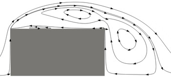
For the numerical simulations, a cell-centred fully unstructured finite volume (FV) code called Panta Rhei was employed using the PETSc library (Balay et al. Reference Balay, Abhyankar, Adams, Brown, Brune, Buschelman, Dalcin, Eijkhout, Gropp and Kaushik2016) for the algebraic solvers. The coupling between pressure and velocity was achieved via the PISO algorithm (Issa Reference Issa1986). The time integration was carried out using a second-order backward method while the spatial central discretisation was of second order. The FV approach allows the mesh to be stretched so as to better refine the grid in regions of the flow where small-scale dynamics are relevant, such as the core of the wake and the separating shear layer. In § 2.3, we show a comparison with experiments and other simulations of mean flow profiles and integral properties of the flow.

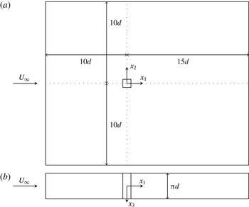
The fluid domain is sketched in figure 2 along with its dimensions and the reference frame. At the inlet, the velocity was set to $U_{\infty }$ , and at the outlet, the one-dimensional advection equation was solved (convective boundary condition). The spanwise boundaries were treated as periodic. At the top and bottom boundaries the Dirichlet condition for pressure and the Neumann condition for the velocity are used to reduce blockage effects, allowing the flow to be entrained across those boundaries.

Figure 2.

Domain dimensions. (a) Side view; (b) top view. The origin of our coordinate system is at the centre of the square prism.

The computational grid used had just under 40 million cells. The length of each side of the square prism in the $(x_{1},x_{2})$ plane was $d$ ; the smallest cell size was $0.0015d$ and was at the corners of the prism. Over each edge, 121 nodes were placed with most nodes being concentrated close to the corners. Near the inlet and top/bottom boundaries, the cell sizes were set to $0.325d$ , while near the outlet, the cell size was $0.065d$ . Appropriate care was taken in connecting the different grid sizes using stretching functions which allowed for a smooth variation of the cell dimensions. The mesh was extruded in the spanwise direction, generating 150 layers. In order to keep the computational requirements as low as possible, the mesh was stretched (in the $x_{1}$ and $x_{2}$ directions), allowing the finer cells to be located in the area around the prism. This ensured appropriate resolution of the thin separating shear layer. In the core of the wake, the resolution was found to be at worse approximately 4 times the Kolmogorov length scale $\unicode[STIX]{x1D702}$ ; in fact, along the centreline, the resolution varied between $3.8\unicode[STIX]{x1D702}$ and $2.9\unicode[STIX]{x1D702}$ at $x_{1}/d=2$ and $x_{1}/d=8$ respectively.

It was found that a maximum value of the Courant–Friedrichs–Lewy number $CFL=u(\unicode[STIX]{x0394}t/\unicode[STIX]{x0394}x)$ of approximately 4 allowed the numerical solution to be stable, and that led to an average of 0.2 across the whole domain. The largest values of the $CFL$ were found in areas where the flow was still laminar. The resulting time step was $0.0025(U_{\infty }/d)$ , which corresponds to approximately 3000 time steps per shedding cycle. In the core of the wake, this value of the time step was smaller by at least one order of magnitude compared with the Kolmogorov time scale.

The numerical computation of all of the terms in (2.1) was carried out by rewriting them as correlations of velocities, pressure and their derivatives between locations $x_{i}^{+}$ and $x_{i}^{-}$ , where the FV approach was used to compute the derivatives.

2.3 Comparison of mean flow and turbulence intensity profiles with the literature

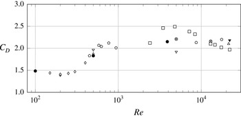
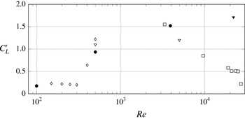
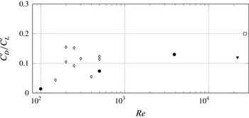
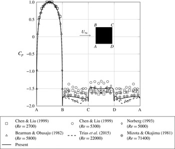
In order to validate our results, we have compared several statistics with those reported in the literature. In the present section, we discuss statistics of the velocity, as well as the shedding frequency associated with the vortex shedding. In appendix A, further comparisons are made for other quantities, such as force coefficients.

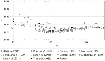
In figure 3, we report values of the normalised shedding frequency, the Strouhal number $St=f_{s}d/U_{\infty }$ (where $f_{s}$ is the shedding frequency), for three values of the Reynolds number $Re$ (100, 500 and 3900). In particular, for the $Re=3900$ case, the value of $St$ was found to be 0.13. Only the $Re=3900$ simulation is used in the remainder of this paper, with the exception of appendix A, where the $Re=100$ and 500 simulations are used for validation purposes.

Figure 3.

Plot of $St$ versus $Re$ from both experiments and DNS. Repeated symbols (for the same  $Re$ ) indicate different experimental/numerical conditions.

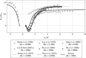
In figures 4–7, we show the variation along the centreline of $U_{1}$ , $u_{1}^{\prime }$ , $u_{2}^{\prime }$ and $u_{3}^{\prime }$ , which are the mean streamwise velocity and the standard deviations of the streamwise, cross-stream and spanwise velocity components respectively. Apart from the DNS results of Arslan et al. (Reference Arslan, El Khoury, Pettersen and Andersson2012) and Trias, Gorobets & Oliva (Reference Trias, Gorobets and Oliva2015), all remaining references refer to experimental results. The DNS of Arslan et al. (Reference Arslan, El Khoury, Pettersen and Andersson2012) employed a code developed for LES simulations. Moreover, they report a resolution in terms of Kolmogorov length scales of approximately $7\unicode[STIX]{x1D702}$ . The DNS of Trias et al. (Reference Trias, Gorobets and Oliva2015), on the other hand, report a resolution of approximately $4\unicode[STIX]{x1D702}$ and, even though they simulate a much larger $Re$ flow, we find a very good agreement between our streamwise profiles and theirs (database available in ref. [36] of their paper).

Significant scatter in the statistics of the velocity is observed when comparing different references. In particular, the estimation of the maximum recirculation velocity and rear-stagnation point appears to be drastically different between experiments and DNS. This is in line with the results reported in Voke (Reference Voke1996) and Sohankar (Reference Sohankar2006), where LES simulations at $Re=22\,000$ are compared with the reference data of Lyn et al. (Reference Lyn, Einav, Rodi and Park1995). On the other hand, significant differences are also observed in the recovery velocity: while the present results and those of Lyn et al. (Reference Lyn, Einav, Rodi and Park1995), Lee & Kim (Reference Lee and Kim2001b ) and Trias et al. (Reference Trias, Gorobets and Oliva2015) show a very slow increase of $U_{1}/U_{\infty }$ along $x_{1}/d$ from a value of approximately $0.6$ at $x_{1}/d\approx 3$ to approximately 0.7 at $x_{1}/d\approx 8$ , others find the mean velocity to be over 20 % higher. It is unlikely that these differences are solely due to wind tunnel blockage and free-stream turbulence. Lyn et al. (Reference Lyn, Einav, Rodi and Park1995), Lee & Kim (Reference Lee and Kim2001b ) and Arslan et al. (Reference Arslan, El Khoury, Pettersen and Andersson2012) reported a blockage of 7 %, but Hu, Zhou & Dalton (Reference Hu, Zhou and Dalton2006) and Trias et al. (Reference Trias, Gorobets and Oliva2015) reported a blockage of approximately 2 %, even though there are differences in their results. The free-stream turbulence, on the other hand, appears to have a more significant effect on $U_{1}/U_{\infty }$ in the experiment of Durão, Heitor & Pereira (Reference Durão, Heitor and Pereira1988), who report 6 % free-stream turbulence; this explains the differences observed in the incoming profiles.

Figure 4.

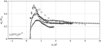
Profile of $U_{1}$ normalised by $U_{\infty }$ along the geometrical centreline for $-2.5<x_{1}/d<10$ . Experimental results from different references are indicated by symbols while the lines indicate numerical (DNS) results.

As seen in figures 5–7, the disparity between the different references in the statistics of fluctuating velocities is even more significant than for $U_{1}/U_{\infty }$ , particularly in the very near wake. The large values of $u_{1}^{\prime }$ observed at $x_{1}/d<-0.5$ in the data of Durão et al. (Reference Durão, Heitor and Pereira1988) are due to their fairly high free-stream turbulence of 6 %. While all references agree that the peak of $u_{1}^{\prime }$ should occur just after $x_{1}\approx d$ , the actual value of $u_{1}^{\prime }/U_{\infty }$ at its peak varies between 0.28 and 0.56. We find the peak value of $u_{1}^{\prime }/U_{\infty }$ to be close to 0.41, which is in agreement with the results of Lyn et al. (Reference Lyn, Einav, Rodi and Park1995) and Trias et al. (Reference Trias, Gorobets and Oliva2015) which were obtained at a larger  $Re$ .

Figure 5.

Profile of $u_{1}^{\prime }=\sqrt{\langle u_{1}^{2}\rangle }$ normalised by $U_{\infty }$ along the geometrical centreline for $-2.5<x_{1}/d<10$ . The legend is the same as in figure 4. Turbulent statistics of Lee & Kim (Reference Lee and Kim2001a ) are shown in Lee & Kim (Reference Lee and Kim2001b ).

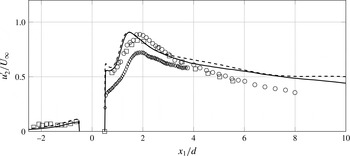
The intensity of cross-stream fluctuations is mostly determined by the shedding. In fact, the distance from the prism to the location of the peak of $u_{2}^{\prime }/U_{\infty }$ is used to define the vortex formation length. Both the present results and those of Trias et al. (Reference Trias, Gorobets and Oliva2015) show a vortex formation length extending to $x_{1}/d\approx 1.5$ , while the experiments of Durão et al. (Reference Durão, Heitor and Pereira1988), Lyn et al. (Reference Lyn, Einav, Rodi and Park1995) and Lee & Kim (Reference Lee and Kim2001b ) place this further downstream, at $x_{1}/d\approx 1.9$ . Apart from the PIV results of Lee & Kim (Reference Lee and Kim2001b ), the peak value of $u_{2}^{\prime }/U_{\infty }$ is reported to be close to 0.9 both in the present results and in Lyn et al. (Reference Lyn, Einav, Rodi and Park1995) and Trias et al. (Reference Trias, Gorobets and Oliva2015) and just over 0.8 in Durão et al. (Reference Durão, Heitor and Pereira1988). Differences are also observed in the decay of $u_{2}^{\prime }/U_{\infty }$ with increasing streamwise distance. Although Lee & Kim (Reference Lee and Kim2001b ) did not measure sufficiently downstream, their results seem to agree with the present DNS and that of Trias et al. (Reference Trias, Gorobets and Oliva2015) in a slower decrease of $u_{2}^{\prime }/U_{\infty }$ with $x_{1}/d$ in comparison with Durão et al. (Reference Durão, Heitor and Pereira1988) and Lyn et al. (Reference Lyn, Einav, Rodi and Park1995).

Figure 6.

Profile of $u_{2}^{\prime }=\sqrt{\langle u_{1}^{2}\rangle }$ normalised by $U_{\infty }$ along the geometrical centreline for $-2.5<x_{1}/d<10$ . The legend is the same as in figure 4. Turbulent statistics of Lee & Kim (Reference Lee and Kim2001a ) are shown in Lee & Kim (Reference Lee and Kim2001b ).

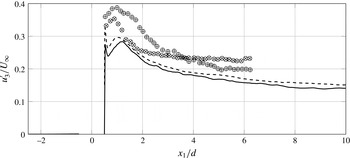
Fewer results are available for the spanwise fluctuating velocity. The hot-wire measurements of Hu et al. (Reference Hu, Zhou and Dalton2006) at two different values of $Re$ show different evolutions of $u_{3}^{\prime }/U_{\infty }$ with $x_{1}/d$ , while the present DNS at $Re=3900$ shows the same profile of $u_{3}^{\prime }/U_{\infty }$ as in Trias et al. (Reference Trias, Gorobets and Oliva2015), whose results refer to $Re=22\,000$ . In the DNS, the peak of $u_{3}^{\prime }/U_{\infty }$ on the centreline appears to be at the same location as the mean stagnation point (where $U_{1}=0$ ).

Figure 7.

Profile of $u_{3}^{\prime }=\sqrt{\langle u_{3}^{2}\rangle }$ normalised by $U_{\infty }$ along the geometrical centreline for $-2.5<x_{1}/d<10$ . The legend is the same as in figure 4.

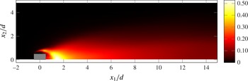
Finally, we show in figure 8 the contour of the normalised turbulent kinetic energy $((u_{1}^{\prime 2}+u_{2}^{\prime 2}+u_{3}^{\prime 2})/2)/U_{\infty }^{2}$ . The peak turbulent kinetic energy occurs at the centreline, due to the large contribution of $u_{2}^{\prime }$ , which also peaks at the centreline. However, it is possible to see another peak (of smaller magnitude) roughly at the stagnation point in between the two large recirculation bubbles at the top/bottom and back (see figure 37 in appendix A). This is most likely due to the flapping of the shear layer as it also corresponds to a peak in $u_{1}^{\prime }/U_{\infty }$ .

Figure 8.

Contour of mean turbulent kinetic energy normalised by $U_{\infty }^{2}$ .

The convergence of the one-point statistics in this section and of two-point statistics such as those in the following sections is presented in appendix B.

3.1 Energy spectra in the frequency domain and Taylor’s hypothesis

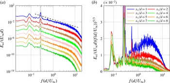
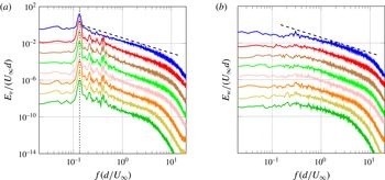
We start by looking at turbulence spectra in the region of the flow where we study the scale-by-scale energy budget (2.1) in the next section. The energy spectra at several locations along the centreline are shown in figures 9(a), 10(a) and 10(b) for the streamwise, cross-stream and spanwise components of the fluctuating velocity respectively. At these locations, the spectra display a power law that is close to $-5/3$ over a substantial range of frequencies at $x_{1}/d=2$ . As the distance $x_{1}$ from the prism increases, this power law deteriorates while the range of frequencies narrows. This is in spite of the flow becoming more homogeneous and undergoing an increase in local Reynolds number. In figure 9(b), the $5/3$ compensated spectra of the streamwise fluctuations are shown in a linear-logarithmic plot to highlight that the spectra are close to a $-5/3$ power law over just under a decade of frequencies, particularly at $x_{1}=2d$ , which is located straight after the peak of turbulent kinetic energy (as seen in figure 8). As will become fully clear in the following section, this observation is in line with the comment made by Kraichnan (Reference Kraichnan1974) that such a power law is observed in regions of flows where Kolmogorov’s theory is not expected to hold. Several other authors have reported such a power law in simulations and experiments on planar wakes (see, e.g., Cantwell & Coles Reference Cantwell and Coles1983; Ong & Wallace Reference Ong and Wallace1996; Kravchenko & Moin Reference Kravchenko and Moin2000; Ma, Karamanos & Karniadakis Reference Ma, Karamanos and Karniadakis2000; Braza et al. Reference Braza, Perrin and Hoarau2006; Wissink & Rodi Reference Wissink and Rodi2008; Lehmkuhl et al. Reference Lehmkuhl, Rodríguez, Borrell and Oliva2013; Trias et al. Reference Trias, Gorobets and Oliva2015) at comparable distances from the wake generator (on the centreline) and similar Reynolds numbers.

Less reported by previous authors, however, is the fact that the range of frequencies over which a power law is observed appears to decrease with increasing downstream distance, in agreement with a similar observation made by Laizet et al. (Reference Laizet, Nedić and Vassilicos2015) in near-field grid-generated turbulence. It is also worth mentioning that the local Taylor-length-based Reynolds number $Re_{\unicode[STIX]{x1D706}}=u_{1}^{\prime }\unicode[STIX]{x1D706}/\unicode[STIX]{x1D708}$ , where $\unicode[STIX]{x1D706}=\sqrt{15(\unicode[STIX]{x1D708}/\unicode[STIX]{x1D700})}u_{1}^{\prime }$ , increases from approximately 120 at $x_{1}/d=2$ to approximately 170 at $x_{1}/d=10$ . This is a first indication that these near $-5/3$ power laws do not have much to do with Kolmogorov theory, where an increase in Reynolds number is expected to lead to a broader inertial range.

Figure 9.

Power spectrum densities of streamwise fluctuating velocity at eight locations on the centreline (different locations are offset by one decade) normalised by $U_{\infty }d$ . In (a), the dashed line indicates a slope of $-5/3$ and the dotted line indicates $f=2f_{s}$ ; in (b), compensated spectra are plotted in linear-logarithmic axes.

Figure 10.

Power spectrum densities, normalised by $U_{\infty }d$ , of the cross-stream and spanwise velocity components, (a) and (b) respectively (different locations are offset by one decade). See figure 9 for the legend. The dashed line indicates a slope of $-5/3$ . In (a), the dotted line indicates $f=f_{s}$ .

Due to the predominantly planar nature of the vortex shedding, only the spectra of the streamwise and cross-stream components display pronounced peaks (figures 9 a and 10 a), while this is not the case for the spectra of spanwise fluctuations (figure 10 b). For the streamwise component, the peak appears at $2f_{s}$ , while for the cross-stream component, the peak occurs at $f_{s}$ . This is due to the alternating vortices shed from the top and bottom sides having spanwise vorticity of opposite signs, thus inducing on the centreline streamwise fluctuations in the same direction but cross-stream fluctuations in opposite directions.

The $-5/3$ power law spectrum obtained by the Kolmogorov theory is for wavenumber spectra (Obukhov Reference Obukhov1941), not frequency spectra. The conversion from wavenumber to frequency required to interpret spectra obtained from velocity data collected over time at a particular point in space is usually based on Taylor’s frozen turbulence hypothesis (introduced in Taylor Reference Taylor1935). According to this hypothesis, high enough frequencies $f$ are related to high enough wavenumbers $k$ by $k=2\unicode[STIX]{x03C0}f/U_{c}$ , where $U_{c}$ is a convection velocity, usually the mean flow velocity at the data collection point. Given that we find well-defined power laws in our frequency spectra with exponents more or less close to $-5/3$ , it makes sense to test the validity of Taylor’s hypothesis at those points where these frequency spectra were found.

To verify Taylor’s hypothesis, we follow the approach of Laizet et al. (Reference Laizet, Nedić and Vassilicos2015) and compute the correlation coefficient

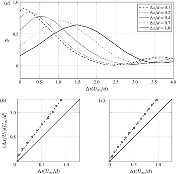
where the velocity component $u_{1}$ is of course also a function of $x_{2}$ and $x_{3}$ in principle but the correlation is evaluated at $x_{2}=x_{3}=0$ . In figure 11(a), $\unicode[STIX]{x1D70C}_{u}$ is plotted for $x_{1}/d=2$ and for five different values of the spatial offset $\unicode[STIX]{x0394}x$ . Even at separations as large as $\unicode[STIX]{x0394}x/d=1$ , there is a strong correlation of the velocity signals. The peaks of the correlation $\unicode[STIX]{x1D70C}_{u}$ can be used to compute $U_{c}$ by taking the ratio between the values of $\unicode[STIX]{x0394}x$ and $\unicode[STIX]{x0394}t$ where these peaks occur.

Figure 11.

In (a), the correlation coefficient (3.1) at $x_{1}/d=2$ on the centreline is plotted for different separations $\unicode[STIX]{x0394}x$ . In (b,c), the symbols indicate the locations of the peaks of (3.1) at both $x_{1}/d=2$  (b) and $x_{1}/d=4$  (c) on the centreline, the full lines indicate the slope $U_{c}/U_{1}=1$ and the dashed lines indicate linear fits to the data.

As shown in figure 11(b,c), there does seem to be a linear relationship between $\unicode[STIX]{x0394}x$ and $\unicode[STIX]{x0394}t$ , suggesting that $U_{c}$ is well defined, which supports the validity of the Taylor hypothesis. As is also clear in figure 11(b,c), $U_{c}$ is slightly larger than the mean flow velocity on the centreline. For example, we have found the values $U_{c}/U_{\infty }\approx 0.67$ and $U_{c}/U_{\infty }\approx 0.83$ at the two centreline locations $x_{1}/d=2$ and $x_{1}/d=4$ respectively, which, as can be seen in figure 4, are indeed larger than $U_{1}$ at the same locations. In fact, $U_{c}$ appears to be close to the convection velocity of the large-scale vortices as reported by Bloor & Gerrard (Reference Bloor and Gerrard1966) and Zhou & Antonia (Reference Zhou and Antonia1992). Similar conclusions can be reached for the components $u_{2}$ and $u_{3}$ of the fluctuating velocity in terms of a correlation coefficient defined as in (3.1) but for $u_{2}$ and $u_{3}$ respectively. In fact, we find $U_{c}(x_{1},0,0)\approx 1.3U_{1}(x_{1},0,0)$ for all three fluctuating velocity components in the range $x_{1}/d\geqslant 3$ , and $U_{c}/U_{1}$ slightly higher but under or close to $1.4$ at $x_{1}=2d$ on the centreline. While many other considerations regarding the conversion from frequency to wavenumber can arise (see Lumley Reference Lumley1965; Wyngaard & Clifford Reference Wyngaard and Clifford1977), it is beyond the scope of this paper to delve into such issues. The point of this limited space–time analysis has simply been to confer a little more substance to our observation of near $-5/3$ power law energy spectra by providing some evidence in favour of the Taylor frozen turbulence hypothesis which therefore suggests that the power law frequency spectra that we have observed may be reflections of similar underlying wavenumber spectra. In the following subsection, we briefly report on second-order structure functions as they are Fourier analogues of wavenumber spectra.

3.2 Second-order structure functions and corresponding spectra

Our supporting evidence for the Taylor hypothesis is limited to spatial separations $r_{1}$ in the streamwise direction and cannot be expected to be valid in other directions. We therefore extract from our DNS data second-order structure functions $\langle \unicode[STIX]{x1D6FF}u_{i}^{2}\rangle$ for $i=1,2,3$ as functions of $(r_{1},0,0)$ at various locations $x_{1}$ on the centreline. Given the near $-5/3$ power law scalings observed in the frequency spectra, one might expect these second-order structure functions to have a near $2/3$ power law dependence on $r_{1}$ in an intermediate range of scales. The power law range in the frequency spectra is, at most, approximately $0.5<fd/U_{\infty }<3$ . Assuming that we can apply Taylor’s hypothesis and therefore $r_{1}f=U_{c}$ , this power law range of frequencies translates to $(1/3)U_{c}/U_{\infty }<r_{1}/d<2U_{c}/U_{\infty }$ , i.e. typically around $0.25<r_{1}/d<1.5$ . 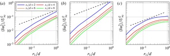However, as seen in figure 12, the structure functions $\langle \unicode[STIX]{x1D6FF}u_{i}^{2}\rangle$ (for $i=1,2,3$ ) do not have a near $2/3$ power law in this range. In fact, the approximate slopes of $\log (\langle \unicode[STIX]{x1D6FF}u_{1}^{2}\rangle )$ and $\log (\langle \unicode[STIX]{x1D6FF}u_{2}^{2}\rangle )$ vastly exceed $2/3$ , while the $\log (\langle \unicode[STIX]{x1D6FF}u_{3}^{2}\rangle )$ curve reaches it only tangentially in this range.

The striking difference between the planar structure functions $\langle \unicode[STIX]{x1D6FF}u_{1}^{2}\rangle$ and $\langle \unicode[STIX]{x1D6FF}u_{2}^{2}\rangle$ and the spanwise structure function $\langle \unicode[STIX]{x1D6FF}u_{3}^{2}\rangle$ as well as the very steep growth of the planar structure functions compared with $r_{1}^{2/3}$ can be explained in terms of the vortex shedding which is clearly visible in figures 9(a) and 10(a) but absent in figure 10(b). The lack of a clear $2/3$ power law in the $r_{1}$ dependence of $\langle \unicode[STIX]{x1D6FF}u_{3}^{2}\rangle$ is consistent with the observation sometimes made (Frisch Reference Frisch1995; Lindborg Reference Lindborg1999) that the range of wavenumbers (or frequencies) over which a well-defined $-5/3$ power law is observed is in general larger than the range of scales over which a $2/3$ power law for the second-order structure is clearly present (see also Antonia et al. Reference Antonia, Smalley, Zhou, Anselmet and Danaila2003). We now illustrate these two points in terms of a simple example.

Figure 12.

Second-order structure functions of the three different velocity components along $r_{1}$ at three different locations on the centreline. The dashed line indicates a slope of $2/3$ .

We consider a model spectrum (see Pope Reference Pope2000) given by

where $E_{0}(k)$ and $E_{\unicode[STIX]{x1D702}}(k)$ characterise the low- and high-wavenumber behaviour of the spectrum respectively and are constant in the intermediate range of wavenumbers $k$ where $E_{u}(k)\propto k^{-5/3}$ . We take functions $E_{0}(k)$ and $E_{\unicode[STIX]{x1D702}}(k)$ ,

so that $E_{u}(k)\propto k^{-5/3}$ in the range $k_{0}\ll k\ll k_{\unicode[STIX]{x1D702}}$ . We chose the constants $c_{0}$ and $c_{\unicode[STIX]{x1D702}}$ and the inner and outer wavenumbers $k_{0}$ and $k_{\unicode[STIX]{x1D702}}$ such that the spectrum takes the form shown in figure 13. In the same figure, we also plot another model spectrum obtained in the exact same way but with highly amplified energy around a wavenumber $k_{s}$ (both spectra integrate to the same total kinetic energy). We do so via

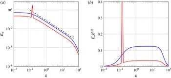
where $A$ is an amplification factor, $k_{s}$ is the wavenumber associated with the shedding and $\unicode[STIX]{x0394}k_{s}$ represents the spread of the spectral peak. Equation (3.4) attempts to mimic the model introduced in Thiesset et al. (Reference Thiesset, Danaila and Antonia2014) in scale space, which is effectively associated with a peak in spectral space. The $-5/3$ power law is well defined for over one decade of wavenumbers in both model spectra, as made clear in figure 13(b), where the spectra have been compensated by $k^{5/3}$ .

Figure 13.

Models of a spectrum with one decade inertial range. One of the spectra (in red) is amplified at a given wavenumber. In (b), the spectra are compensated by $k^{5/3}$ .

Figure 14.

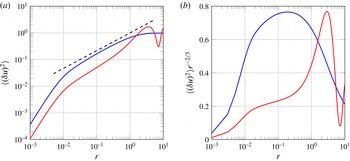
Second-order structure functions obtained by the inverse Fourier transform of the spectra plotted in figure 13. In (b), the structure functions are compensated by $r^{-2/3}$ .

We now calculate the second-order structure functions corresponding to the two model spectra of figure 13 from

where ${\mathcal{F}}^{-1}$ denotes an inverse Fourier transform. These structure functions are plotted in figure 14 and one can make two clear observations. First, there is no $2/3$ power law even though there is a well-defined $-5/3$ power law in the spectrum from which these structure functions are derived. At best, $\langle \unicode[STIX]{x1D6FF}u^{2}\rangle$ reaches $r^{2/3}$ only tangentially in the case of the model spectrum without the shedding peak. This is similar to our result plotted in figure 12 for $\langle \unicode[STIX]{x1D6FF}u_{3}^{2}\rangle$ , which concerns spanwise fluctuating velocities unaffected by the planar vortex shedding. Second, the vortex shedding peak of one of the two model spectra has introduced a growth much steeper than a $2/3$ power law in the corresponding structure function. As noted by Thiesset et al. (Reference Thiesset, Danaila and Antonia2014), one should indeed expect the effect of the shedding on the second-order structure function to be reflected by a sinusoid-like function. Figure 14 demonstrates that this sinusoid can, in fact, very significantly contaminate the power law range of the structure function even when the corresponding energy spectrum has a well-defined $k^{-5/3}$ range over more than a decade. The resulting structure function is much steeper than a $2/3$ power law in the range of scales that corresponds to the $-5/3$ part of the spectrum. This is similar to our results plotted in figure 12 for $\langle \unicode[STIX]{x1D6FF}u_{1}^{2}\rangle$ and $\langle \unicode[STIX]{x1D6FF}u_{2}^{2}\rangle$ , which concerns planar fluctuating velocities that are affected by vortex shedding.

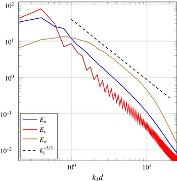
Inverting (3.5) and using it to obtain the spectra that correspond to the structure functions in figure 12 does return $-5/3$ power law spectra over a range of wavenumbers comparable to the range of frequencies where figures 9(a), 10(a) and 10(b) exhibit $-5/3$ power laws (see figure 15).

Figure 15.

Energy spectra in wavenumber obtained by Fourier transform of the correlation functions of each velocity component at $x_{1}/d=4$ .

In conclusion, the evidence presented in this and the previous subsections supports the view that there is an underlying approximate $r_{1}^{2/3}$ dependence in all three second-order structure functions on the centreline of our DNS but over a very short $r_{1}$ range. In the case of the streamwise and cross-stream structure functions, this range is totally overshadowed by the vortex shedding signature. The energy spectrum amplifies the power law region and makes it appear as a clear near $-5/3$ power law over a wide range of frequencies/wavenumbers while at the same time disentangling it from the vortex shedding signature. However, these near $-5/3$ power law spectra cannot be obviously explained by the Kolmogorov theory: their range appears to reduce rather than increase with Reynolds number and, as we show in the following subsection, there is no isotropy in that range.

3.3 Second-order structure functions and isotropy

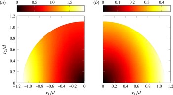
In figure 16, $\langle \unicode[STIX]{x1D6FF}q^{2}\rangle$ is plotted for $r_{3}=0$ at two different locations in space. The distribution of $\langle \unicode[STIX]{x1D6FF}q^{2}\rangle$ in scale space shows that the energy is distributed anisotropically in the range $0.2\leqslant r/d$ , which includes most of the range $0.15<r_{1}/d<1.5$ where the $-5/3$ power laws are observed. Comparison of figure 16(a) with figure 16(b) shows that there is an overall decrease of the energy and suggests some tendency towards isotropy with increasing downstream position.

Figure 16.

Distribution of $\langle \unicode[STIX]{x1D6FF}q^{2}\rangle$ normalised by $U_{\infty }^{2}$ in scale space on the geometrical centreline at $x_{1}/d=2$ and $x_{1}/d=8$ in (a) and (b) respectively.

Figure 17.

The $i\text{th}$ component of the second-order structure function $\langle \unicode[STIX]{x1D6FF}u_{i}^{2}\rangle$ normalised by $U_{\infty }^{2}$ on the centreline at $x_{1}/d=2$ .

The structure functions associated with each velocity component at $x_{1}/d=2$ are shown in figure 17. It is clear that the large values of $\langle \unicode[STIX]{x1D6FF}q^{2}\rangle$ observed in figure 16 are associated with the large contribution of $\langle \unicode[STIX]{x1D6FF}u_{2}^{2}\rangle$ compared with the other two components. In fact, one could have anticipated that, at least for orientations aligned with the mean flow direction, the structure function associated with the vertical fluctuations would have a significant contribution to the total energy, as comparison of figure 6 with figures 5 and 7 shows that it is that component that contributes the most to the turbulent kinetic energy.

The plots in figure 17 show very distinct anisotropy except for $\langle \unicode[STIX]{x1D6FF}u_{3}^{2}\rangle$ , which is unaffected by the vortex shedding. As seen at the start of this section, the frequency spectra of $u_{1}$ and $u_{2}$ show a persistent peak at the frequency associated with the vortex shedding, indicating that the anisotropy observed in figures 16 and 17 is most likely due to the coherent motion, as also suggested by Thiesset, Danaila & Antonia (Reference Thiesset, Danaila and Antonia2013b ). However, it is not easy with the tools used in this paper to disentangle the shedding-induced anisotropy from an underlying potentially isotropic small-scale turbulence which may or may not be amenable to the Kolmogorov framework. We leave this issue for a future study based on a triple decomposition of the velocity field which distinguishes between coherent and incoherent fluctuations. In the following section, we proceed with the study of the various terms in the KHMH equation, which in fact brings further, and in fact more substantial, evidence of anisotropy.

4.1 Forward and inverse cascades by nonlinear interactions

The nonlinear interscale transfer rate $\unicode[STIX]{x1D6F1}$ is the divergence in scale space of the nonlinear interscale flux vector $\langle \unicode[STIX]{x1D6FF}\boldsymbol{u}\unicode[STIX]{x1D6FF}q^{2}\rangle$ . The orientation of this flux is directly linked to the concept of energy cascade as it can characterise the direction where energy flows in scale space. In the context of the Richardson–Kolmogorov equilibrium cascade and the assumption of local isotropy, this flux has a radial component that points from large to small separations for any orientation.

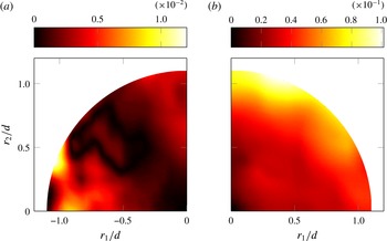
From now on, we concentrate attention on four centreline locations, namely $x_{1}/d=2$ , 4, 6, 8, all far enough from the recirculation region and from the downstream end of our DNS domain; see figures 2 and 4. In figure 18, we plot the nonlinear interscale flux in scale space at two centreline locations. The figure shows the direction of the vector $\langle \unicode[STIX]{x1D6FF}\boldsymbol{u}\unicode[STIX]{x1D6FF}q^{2}\rangle$ , with its magnitude in the background. While the magnitude of $\langle \unicode[STIX]{x1D6FF}\boldsymbol{u}\unicode[STIX]{x1D6FF}q^{2}\rangle$ is, in general, larger at large separations, its distribution in scale space is far from isotropic. Moreover, the orientation of $\langle \unicode[STIX]{x1D6FF}\boldsymbol{u}\unicode[STIX]{x1D6FF}q^{2}\rangle$ varies drastically with the orientation of the scale vector $\boldsymbol{r}$ , suggesting that $\langle \unicode[STIX]{x1D6FF}q^{2}\rangle$ is, on average, redistributed in scale space, rather than solely transferred from large to small  $r$ .

Figure 18.

Interscale flux of energy due to nonlinear interactions $\langle \unicode[STIX]{x1D6FF}\boldsymbol{u}\unicode[STIX]{x1D6FF}q^{2}\rangle$ at $x_{1}/d=2$ (a) and $x_{1}/d=8$ (b) for $r_{3}=0$ . The arrows indicate the orientation of the vector $\langle \unicode[STIX]{x1D6FF}\boldsymbol{u}\unicode[STIX]{x1D6FF}q^{2}\rangle$ and the contour indicates the magnitude normalised by $U_{\infty }^{3}$ .

It should be noticed how, at $x_{1}=2$ , the flux is directed outwards (from small to large $r/d$ ) at separations close to the $r_{2}=0$ axis. At a location further downstream ( $x_{1}/d=8$ ), the fluxes have rotated by $90^{\circ }$ and the flux is now directed inwards (from large to small $r/d$ ) at separations close to the $r_{2}=0$ axis (in agreement with the measurements of Thiesset et al. Reference Thiesset, Danaila and Antonia2014) but outwards at separations close to the $r_{1}=0$ axis.

A necessary condition for a forward or inverse cascade is that the radial component

of the flux $\langle \unicode[STIX]{x1D6FF}\boldsymbol{u}\unicode[STIX]{x1D6FF}q^{2}\rangle$ is positive or negative.

While the sign of $\langle \unicode[STIX]{x1D6FF}u_{r}\unicode[STIX]{x1D6FF}q^{2}\rangle$ indicates whether the flux is from large to small (negative) or small to large (positive) scales, it is not sufficient to characterise the energy cascade as being direct or inverse. For the energy to be truly cascading from large to small scales, it is necessary that negative values of $\langle \unicode[STIX]{x1D6FF}u_{r}\unicode[STIX]{x1D6FF}q^{2}\rangle$ be associated with negative values of the radial component of the nonlinear interscale transfer rate $\unicode[STIX]{x1D6F1}$ written in cylindrical coordinates (with the cylindrical axis in the spanwise direction), i.e.

Conversely, for the energy to be cascading from small to large scales, positive values of $\langle \unicode[STIX]{x1D6FF}u_{r}\unicode[STIX]{x1D6FF}q^{2}\rangle$ must be associated with positive values of $\unicode[STIX]{x1D6F1}_{r}$ . 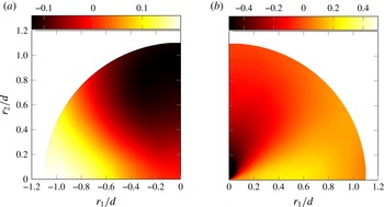In other words, the radial flux $\langle \unicode[STIX]{x1D6FF}u_{r}\unicode[STIX]{x1D6FF}q^{2}\rangle$ is only responsible for an accumulation (depletion) of energy at a given separation vector $\boldsymbol{r}$ if the gradient given by (4.2) is positive (negative) at that separation vector. Figures 19 and 20 map (4.1) and (4.2) in scale space at the same locations as figure 18.

Figure 19.

Radial contributions to the nonlinear interscale flux (a) and transfer (b) of $\langle \unicode[STIX]{x1D6FF}q^{2}\rangle$ at $x_{1}/d=2$ , (4.1) and (4.2) respectively.

Figure 20.

Radial contributions to the nonlinear interscale flux (a) and transfer (b) of $\langle \unicode[STIX]{x1D6FF}q^{2}\rangle$ at $x_{1}/d=8$ , (4.1) and (4.2) respectively.

It is now clear that figures 19 and 20 suggest a coexistence of forward and inverse nonlinear cascades at both centreline locations $x_{1}/d=2$ and $x_{1}/d=8$ . In agreement with figure 18, the orientations where these two simultaneous cascades operate differ at these two locations. The cascade appears inverse in the streamwise and forward in the cross-stream direction at $x_{1}/d=2$ , but forward in the streamwise and inverse in the cross-stream direction at $x_{1}/d=8$ . It is important to note that these local, in scale space, inverse cascade behaviours coexist with energy spectra characterised by near $-5/3$ power laws, in particular at $x_{1}/d=2$ where these power laws are closest to $-5/3$ and the inverse cascade behaviour is in the streamwise direction where the spectra are effectively evaluated. Such coexistence as the one at $x_{1}/d=2$ was already observed in Gomes-Fernandes et al. (Reference Gomes-Fernandes, Ganapathisubramani and Vassilicos2015) in the very near field of a different turbulent flow, while the experiments of Thiesset et al. (Reference Thiesset, Danaila and Antonia2014) did not allow capture of these phenomena because their measurements were carried out further downstream and because their measurement apparatus was limited to $r_{2}=0$ .

Figure 21.

Illustration of the $r_{3}=0$ plane for $x_{i}$ aligned with the centreline. The angle $\unicode[STIX]{x1D703}$ indicates the angle over which the orientations of $r_{i}$ are averaged.

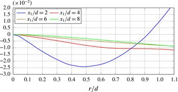
Given the presence of simultaneous forward and inverse cascade behaviours along different scale-space orientations, it is important to average over these orientation angles (as illustrated in figure 21) and work out whether the nonlinear cascade is, on average, forward or inverse. The orientation-averaged radial component of the nonlinear interscale flux, i.e. $\langle \unicode[STIX]{x1D6FF}u_{r}\unicode[STIX]{x1D6FF}q^{2}\rangle ^{a}=(1/2\unicode[STIX]{x03C0})\int _{0}^{2\unicode[STIX]{x03C0}}\,\text{d}\unicode[STIX]{x1D703}\langle \unicode[STIX]{x1D6FF}u_{r}\unicode[STIX]{x1D6FF}q^{2}\rangle$ (where $\unicode[STIX]{x1D703}$ is the scale-space orientation angle, i.e. $r_{1}/r=\cos \unicode[STIX]{x1D703}$ , see figure 21), is a function of $r$ and is plotted in figure 22 for centreline locations $x_{1}/d=2$ , 4, 6, 8. Apart from the location closest to the cylinder ( $x_{1}/d=2$ ), $\langle \unicode[STIX]{x1D6FF}u_{r}\unicode[STIX]{x1D6FF}q^{2}\rangle ^{a}$ remains negative over all scales investigated, and even at $x_{1}/d=2$ it remains negative over a wide range of scales, $r/d<0.86$ . This means that the nonlinear cascade is forward on average on the centreline near field $2\leqslant x_{1}/d\leqslant 8$ of a square prism turbulent wake, and results from combined forward and inverse cascades in different directions, as exemplified by figures 19 and 20.

Figure 22.

Orientation-averaged radial component of the nonlinear interscale flux $\langle \unicode[STIX]{x1D6FF}u_{r}\unicode[STIX]{x1D6FF}q^{2}\rangle ^{a}$ at four different locations along the centreline.

We distinguish between ‘forward/inverse cascades’ and ‘forward/inverse cascade behaviours’ because the possibility remains that turbulent flow inhomogeneities, in particular at the larger scales but a priori even potentially at some smaller scales, may have some contribution to the behaviour of the interscale flux vector $\langle \unicode[STIX]{x1D6FF}\boldsymbol{u}\unicode[STIX]{x1D6FF}q^{2}\rangle$ . Equally, inhomogeneity may be a priori and at least partially responsible for the predominantly negative values of $\langle \unicode[STIX]{x1D6FF}u_{r}\unicode[STIX]{x1D6FF}q^{2}\rangle ^{a}$ , indicating a forward cascade on average. Untangling of the inhomogeneity from the actual cascade contributions is a delicate and important question which will need to be carefully addressed in future works.

4.2 Contributions of the different terms in the KHMH equation

As the KHMH equation clearly illustrates, the nonlinear cascade does not happen in isolation unless the length scales considered are so small that direct viscous diffusion effects matter and/or the turbulence is sufficiently inhomogeneous for at least one of the production ${\mathcal{P}}$ , the linear interscale transfer rate $\unicode[STIX]{x1D6F1}_{U}$ , the spatial transport ${\mathcal{T}}_{u}$ and the pressure term ${\mathcal{T}}_{p}$ to be significant. The type of inhomogeneity that causes the advection term ${\mathcal{A}}$ to be non-negligible when averaging is over time and ${\mathcal{A}}_{t}=0$ by construction is a reflection of the unsteady nature of the small-scale turbulence in the frame following a mean flow. In this subsection, we examine all of these additional processes in order to establish the energy exchange context in which the nonlinear cascade of the previous section occurs.

We first confirmed that the viscous terms ${\mathcal{D}}_{x}$ and ${\mathcal{D}}_{r}$ are indeed negligible in (2.1), except at very small scales (comparable to or smaller than the local Taylor microscale, which is typically around $d/10$ at the centreline positions investigated) (see appendix B in Valente & Vassilicos Reference Valente and Vassilicos2015). We therefore now deal with $\unicode[STIX]{x1D6F1}$ and ${\mathcal{T}}_{p}$ , ${\mathcal{A}}$ and ${\mathcal{T}}_{u}$ , and ${\mathcal{P}}$ and $\unicode[STIX]{x1D6F1}_{U}$ .

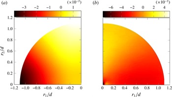
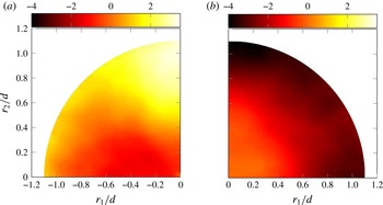
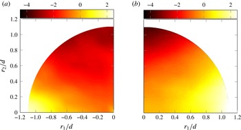
In figures 23 and 24, both $\unicode[STIX]{x1D6F1}$ and ${\mathcal{T}}_{p}$ are plotted in scale space at two different locations on the centreline ( $x_{1}/d=2$ and $x_{1}/d=8$ respectively). In § 2.1, ${\mathcal{T}}_{p}$ is written as $-(\unicode[STIX]{x2202}\langle \unicode[STIX]{x1D6FF}u_{i}\unicode[STIX]{x1D6FF}p\rangle /\unicode[STIX]{x2202}x_{i})/2$ ; however, another possible formulation is $-(\unicode[STIX]{x2202}\langle \unicode[STIX]{x1D6FF}u_{i}(p^{+}+p^{-})\rangle /\unicode[STIX]{x2202}r_{i})/4$ , which resembles the expression for $\unicode[STIX]{x1D6F1}$ with $-(p^{+}+p^{-})$ taking the place of $\unicode[STIX]{x1D6FF}q^{2}$ . At both locations ( $x_{1}/d=2$ and $x_{1}/d=8$ ), $\unicode[STIX]{x1D6F1}$ acts simultaneously as a source ( $\unicode[STIX]{x1D6F1}<0$ ) and a sink term ( $\unicode[STIX]{x1D6F1}>0$ ) in (2.1). However, ${\mathcal{T}}_{p}$ is initially (at $x_{1}/d=2$ ) a sink term ( ${\mathcal{T}}_{p}<0$ ) at all orientations and amplitudes of $\boldsymbol{r}$ , while further downstream (at $x_{1}/d=8$ ), just like $\unicode[STIX]{x1D6F1}$ , it acts as both a source ( ${\mathcal{T}}_{p}>0$ ) and a sink term ( ${\mathcal{T}}_{p}<0$ ) in (2.1).

Figure 23.

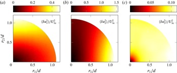
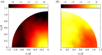
Nonlinear interscale transfer $\unicode[STIX]{x1D6F1}$ (a) and pressure term ${\mathcal{T}}_{p}$ (b) normalised by $\unicode[STIX]{x1D700}_{r}$ at $x_{1}/d=2$ on the centreline.

Figure 24.

Nonlinear interscale transfer $\unicode[STIX]{x1D6F1}$ (a) and pressure term ${\mathcal{T}}_{p}$ (b) normalised by $\unicode[STIX]{x1D700}_{r}$ at $x_{1}/d=8$ on the centreline.

It is important to distinguish $\unicode[STIX]{x1D6F1}$ from $\unicode[STIX]{x1D6F1}_{r}$ (see (4.2)) shown in figures 19 and 20. In § 4.1, $\unicode[STIX]{x1D6F1}_{r}$ is used to describe how $\unicode[STIX]{x1D6FF}q^{2}$ is exchanged from large to small scales (and vice versa). However, the term that actually appears in the budget of $\langle \unicode[STIX]{x1D6FF}q^{2}\rangle$ is $\unicode[STIX]{x1D6F1}$ , the divergence in scale space of the nonlinear interscale flux $\langle \unicode[STIX]{x1D6FF}\boldsymbol{u}\unicode[STIX]{x1D6FF}q^{2}\rangle$ . Figures 23 and 24 reveal that the nonlinear interactions can act as a source of $\langle \unicode[STIX]{x1D6FF}q^{2}\rangle$ independently from the orientation of $\langle \unicode[STIX]{x1D6FF}u_{i}\unicode[STIX]{x1D6FF}q^{2}\rangle$ , i.e. it is not necessary to have a forward cascade ( $\langle \unicode[STIX]{x1D6FF}u_{r}\unicode[STIX]{x1D6FF}q^{2}\rangle <0$ ) to observe $\unicode[STIX]{x1D6F1}<0$ .

What is also, perhaps, surprising from figure 23 and 24 is how ${\mathcal{T}}_{p}$ loses its somewhat isotropic distribution as $x_{1}$ increases. Moreover, it would appear from figure 24 that there is some correlation at $x_{1}/d=8$ between the distributions of ${\mathcal{T}}_{p}$ and $\unicode[STIX]{x1D6F1}$ in scale space, in agreement with recent results by Yasuda & Vassilicos (Reference Yasuda and Vassilicos2017) for periodic turbulence. The fact that ${\mathcal{T}}_{p}$ remains a significant term in the KHMH equation may not be fully unexpected, from the measurements of Gomes-Fernandes et al. (Reference Gomes-Fernandes, Ganapathisubramani and Vassilicos2015) for example, but it does not seem to have been previously reported. One may anticipate that ${\mathcal{T}}_{p}$ reflects the presence of the coherent vortices associated with the shedding which introduce strong pressure gradients in the flow.

Two other terms that also appear to correlate as the downstream location increases are the terms responsible for transporting $\unicode[STIX]{x1D6FF}q^{2}$ in physical space, ${\mathcal{A}}$ and ${\mathcal{T}}_{u}$ . In figures 25 and 26, these two terms are shown side by side for $x_{1}/d=2$ and $x_{1}/d=8$ respectively. At all separation vectors $\boldsymbol{r}$ considered, one can observe that ${\mathcal{A}}<0$ . This indicates that, regardless of the orientation and amplitude of $\boldsymbol{r}$ , $\langle \unicode[STIX]{x1D6FF}q^{2}\rangle$ decays in the direction of the mean flow. The turbulent transport ${\mathcal{T}}_{u}$ also appears to be predominantly negative, especially at the location closest to the prism.

Figure 25.

Advection ${\mathcal{A}}$ (a) and turbulent transport ${\mathcal{T}}_{u}$ (b) normalised by $\unicode[STIX]{x1D700}_{r}$ at $x_{1}/d=2$ on the centreline.

Figure 26.

Advection ${\mathcal{A}}$ (a) and turbulent transport ${\mathcal{T}}_{u}$ (b) normalised by $\unicode[STIX]{x1D700}_{r}$ at $x_{1}/d=8$ on the centreline.

At $x_{1}/d=2$ , ${\mathcal{A}}$ appears to be roughly independent of the orientation of $r_{i}$ , suggesting that initially the decay of $\langle \unicode[STIX]{x1D6FF}q^{2}\rangle$ depends only on $r=|r_{i}|$ . However, as $x_{1}$ increases and the production term weakens, ${\mathcal{A}}$ appears to tend to map in scale space in a way roughly similar to ${\mathcal{T}}_{u}$ . This suggests the development with downstream distance of a sweeping mechanism (see Tsinober Reference Tsinober2009) whereby small-scale turbulent eddies are transported by the larger turbulent eddies so that a tendency develops for ${\mathcal{A}}$ and ${\mathcal{T}}_{u}$ to more or less balance.

The existence of a strong sweeping correlation between ${\mathcal{A}}$ and ${\mathcal{T}}_{u}$ is supported by the measurements of Gomes-Fernandes et al. (Reference Gomes-Fernandes, Ganapathisubramani and Vassilicos2015), which reveal an even stronger correlation between ${\mathcal{A}}$ and ${\mathcal{T}}_{u}$ than evidenced here (see figure 22 of that paper), albeit in a different turbulent flow configuration, and by the recent DNS of periodic turbulence by Yasuda & Vassilicos (Reference Yasuda and Vassilicos2017).

The two remaining terms to be considered in the KHMH equation are ${\mathcal{P}}$ and $\unicode[STIX]{x1D6F1}_{U}$ , which, unlike the previous terms which reflect inhomogeneity of the turbulence, are associated with inhomogeneity of the mean flow. One therefore expects their contribution in (2.1) to decrease with increasing downstream location, as is indeed observed by comparing figures 27 and 28.

Figure 27.

Production ${\mathcal{P}}$ (a) and linear interscale transfer $\unicode[STIX]{x1D6F1}_{U}$ (b) normalised by $\unicode[STIX]{x1D700}_{r}$ at $x_{1}/d=2$ on the centreline.

Figure 28.

Production ${\mathcal{P}}$ (a) and linear interscale transfer $\unicode[STIX]{x1D6F1}_{U}$ (b) normalised by $\unicode[STIX]{x1D700}_{r}$ at $x_{1}/d=8$ on the centreline.

Apart from the clear decrease in magnitude, it is also clear that the distribution of ${\mathcal{P}}$ undergoes a reorientation in scale space, perhaps similar to the one reported in figure 18 for the interscale flux. The production ${\mathcal{P}}$ appears to be stratified along the $r_{1}$ axis at $x_{1}/d=2$ , presumably as a consequence of the strong mean flow gradients in the streamwise direction very close to the prism (see figure 4). Further downstream, at $x_{1}/d=8$ , ${\mathcal{P}}$ appears to be stratified along the $r_{2}$ axis. The largest variations of mean velocity occur in the cross-stream direction at that position.

It may be interesting to contrast the scale-space maps of ${\mathcal{P}}$ in figures 27 and 28 and those of the interscale flux in figure 18. At both centreline locations, $x_{1}/d=2$ and $x_{1}/d=8$ , the apparently inverse cascading interscale flux which points from small to large scales along $r_{1}$ at $x_{1}/d=2$ and along $r_{2}$ at $x_{1}/d=8$ also points from low to high ${\mathcal{P}}$ values. However, in the $x_{1}/d=2$ case, it does clearly point from high to low ${\mathcal{P}}$ values along the $r_{2}$ axis where the cascade appears to be forward, which does appear to be natural. We must leave the explanation of the non-intuitive relation between inverse cascade and scale-space ${\mathcal{P}}$ map for a future study which may involve all three directions in scale space and a better representation of coherent structures in the scale-by-scale energy balance.

The scale-space map of $\unicode[STIX]{x1D6F1}_{U}$ is mostly determined by the alignment of the mean velocity differences $\unicode[STIX]{x1D6FF}U_{i}$ with the gradient (in scale space) of $\langle \unicode[STIX]{x1D6FF}q^{2}\rangle$ . It should be recalled from figure 16 that the distribution of $\langle \unicode[STIX]{x1D6FF}q^{2}\rangle$ in scale space does not undergo significant changes between the two locations investigated. On the other hand, the components of $\unicode[STIX]{x1D6FF}U_{i}$ can be expected to decrease significantly as the wake spreads and recovers towards $U_{\infty }$ . In fact, $\unicode[STIX]{x1D6FF}U_{1}$ must remain positive for positive $r_{1}$ (as $U_{1}$ increases with $x_{1}$ ) and $\unicode[STIX]{x1D6FF}U_{2}$ must remain negative for positive $r_{2}$ due to the symmetry of the wake.

The results presented in this subsection illustrate how the present turbulent flow does not satisfy Kolmogorov’s 1941 premises of equilibrium, local homogeneity and local isotropy even at separation length scales that correspond to the range where the energy spectra we have presented have well-defined power laws with exponents close to $-5/3$ . The nonlinear cascade occurs in a context where various other processes affecting the turbulent kinetic energy are active, including production, advection and turbulent transport in physical space, correlations between fluctuating velocity differences and differences of pressure gradients, and linear interscale transfer by the mean flow. In the following subsection, we show how these processes balance when we average over planar orientations, thereby reducing the orientation-averaged KHMH equation to $\unicode[STIX]{x1D6F1}^{a}\approx -\unicode[STIX]{x1D700}_{r}^{a}\approx -\unicode[STIX]{x1D700}$ over a growing range of separations $r$ for further downstream centreline positions $x_{1}/d$ (the superscript $a$ indicates an average over planar orientation angles, as illustrated in figure 21). We have ascertained that, at $x_{1}/d=2$ and 8 on the centreline, $\unicode[STIX]{x1D700}_{r}^{a}$ and $\unicode[STIX]{x1D700}$ are very closely equal over the entire range $0\leqslant r/d\leqslant 1.1$ of the figures discussed in the following subsection, so that if the quantities plotted in these figures were normalised by $\unicode[STIX]{x1D700}$ , then these figures would look effectively the same.

4.3 Orientation-averaged KHMH equation

In figure 29, we plot the planar orientation-averaged terms of (2.1) normalised by $\unicode[STIX]{x1D700}_{r}^{a}$ . These plots are shown for two centreline positions, $x_{1}/d=2$ and $x_{1}/d=8$ . At $r=0$ , all terms vanish except $\unicode[STIX]{x1D700}_{r}^{a}$ and ${\mathcal{D}}_{r}^{a}$ , which balance exactly, as can actually be shown analytically. At both positions, the viscous diffusion terms are negligible except at separations $r$ smaller than the Taylor length scale, which is approximately $0.06d$ at $x_{1}/d=2$ and $0.1d$ at $x_{1}/d=8$ . None of the other terms are negligible at separations $r$ larger than the Taylor length scale except $\unicode[STIX]{x1D6F1}_{U}$ at the larger centreline distance. In fact, at $x_{1}/d=2$ , all terms associated with inhomogeneity increase their contribution to (2.1) as $r$ increases.

Figure 29.

Orientation-averaged terms of (2.1) normalised by $\unicode[STIX]{x1D700}_{r}^{a}$ at $x_{1}/d=2$ (a) and $x_{1}/d=8$  (b).

As the distance from the prism is increased, the contribution of $\unicode[STIX]{x1D6F1}_{u}^{a}$ is considerably reduced (as already observed in figure 28). It can also be seen in figure 29 that even at the location furthest from the prism, the effect of the fluctuating pressure, included in ${\mathcal{T}}_{p}^{a}$ , cannot be neglected, in particular at the largest separations. At the furthest of the two locations, it appears that the dependences on $r$ of ${\mathcal{A}}^{a}$ and ${\mathcal{T}}_{u}^{a}$ mirror each other, with a tendency for one to partly balance the other. This behaviour is consistent with the sweeping mechanism referred to in the previous subsection concerning ${\mathcal{A}}$ and ${\mathcal{T}}_{u}$ at $x_{1}/d=8$ .

Finally, at both locations, we find a range of separations $r$ larger than the Taylor length scale where the orientation-averaged KHMH equation reduces to the following couple of approximate balances:

This range of separations where $\unicode[STIX]{x1D6F1}^{a}\approx -\unicode[STIX]{x1D700}_{r}^{a}\approx -\unicode[STIX]{x1D700}$ increases with increasing $x_{1}/d$ is clearly seen in figure 30, where $\unicode[STIX]{x1D6F1}^{a}/\unicode[STIX]{x1D700}_{r}^{a}$ is plotted at four different locations on the centreline ( $x_{1}/d=2$ , 4, 6, 8). In fact, this range of separations covers one decade at $x_{1}/d=4$ , 6, 8, and $\unicode[STIX]{x1D6F1}^{a}\approx -\unicode[STIX]{x1D700}_{r}^{a}\approx -\unicode[STIX]{x1D700}$ appears to increase towards 1 with increasing $x_{1}/d$ in the range of separations where it is constant. The PIV measurements of Gomes-Fernandes et al. (Reference Gomes-Fernandes, Ganapathisubramani and Vassilicos2015) also found that $\unicode[STIX]{x1D6F1}^{a}$ is approximately constant over a range of separations $r$ in the very near field of a different turbulent flow where the inhomogeneity terms of the KHMH equation are also significant and in fact dominant. However, their measurements indicated an apparently different value of $-\unicode[STIX]{x1D6F1}^{a}/\unicode[STIX]{x1D700}_{r}^{a}$ , significantly larger than 1. It is not clear whether their different value of $\unicode[STIX]{x1D6F1}^{a}/\unicode[STIX]{x1D700}_{r}^{a}$ is a result of the measurement limitations of their PIV and of the hypotheses that they were therefore forced to make to extract information on the KHMH equation from their measurements.

Figure 30.

Orientation-averaged nonlinear interscale transfer $\unicode[STIX]{x1D6F1}^{a}$ normalised by $-\unicode[STIX]{x1D700}_{r}^{a}$ at four different locations along the centreline. See figure 22 for legend.

It is important to point out that the near constancy of $\unicode[STIX]{x1D6F1}^{a}$ requires the inclusion of both its in-plane ( $\unicode[STIX]{x1D6F1}_{r}^{a}$ ) and out-of-plane ( $\unicode[STIX]{x1D6F1}_{z}\equiv \unicode[STIX]{x1D6F1}_{3}$ ) components (the angular contribution $\unicode[STIX]{x1D6F1}_{\unicode[STIX]{x1D703}}^{a}=(1/2\unicode[STIX]{x03C0})\int _{0}^{2\unicode[STIX]{x03C0}}(1/r)((\unicode[STIX]{x2202}\langle \unicode[STIX]{x1D6FF}u_{\unicode[STIX]{x1D703}}\unicode[STIX]{x1D6FF}q^{2}\rangle )/\unicode[STIX]{x2202}\unicode[STIX]{x1D703})\,\text{d}\unicode[STIX]{x1D703}$ is zero). This is illustrated in figure 31, where these two components are plotted as functions of  $r$ . Albeit small, the contribution of $\unicode[STIX]{x1D6F1}_{3}^{a}$ is particularly relevant especially at the smaller separations, where both $\unicode[STIX]{x1D6F1}_{r}^{a}$ and $\unicode[STIX]{x1D6F1}_{3}^{a}$ are not constant but contribute to make $\unicode[STIX]{x1D6F1}^{a}=\unicode[STIX]{x1D6F1}_{r}^{a}+\unicode[STIX]{x1D6F1}_{3}^{a}$ constant. It is likely that the inability of the experimental PIV of Gomes-Fernandes et al. (Reference Gomes-Fernandes, Ganapathisubramani and Vassilicos2015) to access all velocity field components may have affected their results.

Figure 31.

Orientation-averaged in-plane and out-of-plane components of $\unicode[STIX]{x1D6F1}$ at $x_{1}/d=8$ .

As a final comment which echoes the last paragraph of § 4.1, the possibility remains that the inhomogeneity of the turbulence might be contributing to the constancy of  $\unicode[STIX]{x1D6F1}^{a}$ .