2. Governing equations and nonlinear structures

We consider an unmagnetized and homogeneous quantum plasma comprising electrons, and positive and negative ions. The nonlinear dynamics of quantum IAWs is governed by (Hass et al. Reference Hass, Garcia, Goedert and Manfredi2003; Misra Reference Misra2009)

where $n_{j}$ , $u_{j}$ , $m_{j}$ are, respectively, the density, velocity and mass of electrons $(j=e)$ , positive ions $(j=+)$ and negative ions $(j=-)$ ; $\hbar$ is Planck’s constant divided by $2{\rm\pi}$ , ${\it\phi}$ is the electrostatic wave potential, $p_{e}$ is the electron pressure, $x$ and $t$ are, respectively, the space and time variables. In equilibrium, the charge neutrality condition reads $n_{e0}+Z_{-}n_{-0}=Z_{+}n_{+0}$ , where $Z_{\pm }$ are the charge states for positive (negative) ions and $n_{j0}$ is the equilibrium number density of the $j$ th species. From the above equations (2.1)–(2.6), we obtain the following normalized set of basic equations:

In the above equations, the ion number density $n_{j}$ is normalized by its equilibrium value $n_{j0}$ , the ion fluid speed $u_{j}$ is normalized by $C_{s}=(k_{B}T_{Fe}/m_{-})^{1/2}$ , where $j=e,+,-$ , and the wave potential ${\it\phi}$ is normalized by $k_{B}T_{Fe}/e$ , where $k_{B}$ is the Boltzmann constant and $T_{Fe}$ is the electron Fermi temperature. The time and space variables are normalized by the plasma period ${{\it\omega}_{Pj}}^{-1}=(m_{j}/4{\rm\pi}n_{j0}e^{2})^{1/2}$ and the Debye radius ${\it\lambda}_{D}=(k_{B}T_{Fe}/4{\rm\pi}n_{j0}e^{2})^{1/2}$ , respectively. Here we assume that the ions are cold, and the electrons obey the equation of state pertaining to a one-dimensional Fermi gas, given by $p_{e}=(m_{e}v_{Fe}^{2}/3n_{e0}^{2})n_{e}^{3}$ , and we introduce the non-dimensional quantum parameter $H=\hbar{\it\omega}_{pe}/k_{B}T_{Fe}$ . Here, $v_{Fe}$ is the electron Fermi velocity, connected to the Fermi temperature $T_{Fe}$ by $m_{e}v_{Fe}^{2}/2=k_{B}T_{Fe}$ . Finally, ${\it\mu}=n_{e0}/Z_{-}n_{-0}$ , ${\it\beta}=Z_{+}n_{+0}/Z_{-}n_{-0}$ , so ${\it\mu}={\it\beta}-1$ , and ${\it\alpha}=Z_{+}m_{-}/Z_{-}m_{+}$ .

To investigate the linear properties of quantum IAWs in PI plasma, we introduce linear perturbations such as $n_{e}=1+{\it\epsilon}n_{e}^{(1)},n_{+}=1+{\it\epsilon}n_{+}^{(1)},n_{-}=1+{\it\epsilon}n_{-}^{(1)},u_{+}=0+{\it\epsilon}u_{+}^{(1)},u_{-}=0+{\it\epsilon}u_{-}^{(1)},{\it\phi}=0+{\it\epsilon}{\it\phi}^{(1)}$ in the set of equations (2.7)–(2.12).

Now, assuming the plane wave solution of the form $\exp [\text{i}(kx-{\it\omega}t)]$ , where $k$ is the wavenumber and ${\it\omega}$ is the frequency, we obtain the dispersion relation as

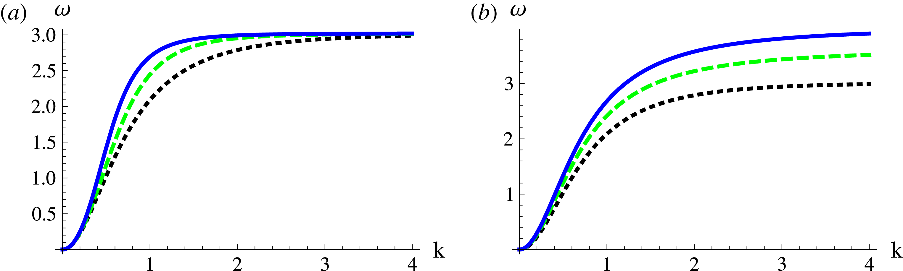
From (2.13) it is seen that the phase velocity is dependent on the quantum correction and other plasma parameters, such as positive to negative ion density ratio ${\it\beta}$ etc. Figure 1 shows the linear variation of normalized wave frequency ${\it\omega}$ as a function of normalized wavenumber $k$ for different values of $H$ and ${\it\beta}$ . It is seen that the wave frequency of the IAW excitations increases with increasing $H$ and ${\it\beta}$ .

Figure 1.

Plot of dispersion relation (2.13) for (a) several values of $H$ : $H=0.5$ (solid line), $H=0.3$ (dashed line), $H=0.1$ (dotted line), where ${\it\alpha}=2.0$ , ${\it\beta}=1.01$ ; and (b) several values of ${\it\beta}$ : ${\it\beta}=1.51$ (solid line), ${\it\beta}=1.31$ (dashed line), ${\it\beta}=1.01$ (dotted line), where ${\it\alpha}=2.0$ , $H=0.1$ .

To study the arbitrary-amplitude IAWs, we suppose that all the quantities depend on ${\it\xi}=x-Mt$ , where $M$ is the Mach number defined as $M=V/C_{s}$ and $V$ is the velocity of the nonlinear structure, as seen in an inertial frame. Defining $n_{e}=A^{2}$ , from (2.7)–(2.12) we obtain the system of second-order differential equations:

The above system of equations (2.14) and (2.15) is equivalent to the following four-dimensional system:

3. Small-amplitude solitary waves

For small amplitude, with the help of (2.14) and (2.15) after some straightforward mathematical manipulation the energy equation can be written as

where the Sagdeev (Reference Sagdeev1966) pseudopotential ${\it\psi}({\it\phi})$ is given by (keeping terms up to ${\it\phi}^{3}$ )

with

and

where

The soliton solution of (3.1) is given by

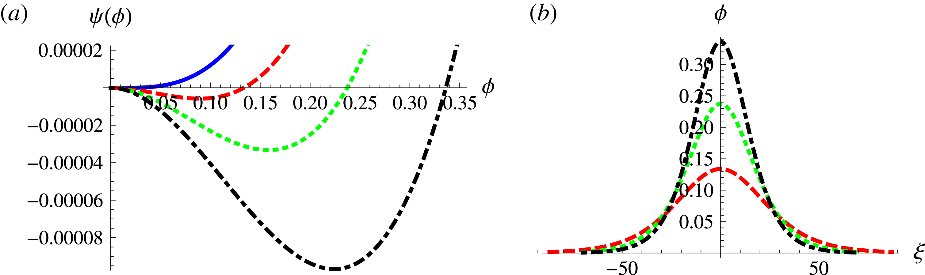
For real solutions in (3.7), we require that $F_{1}<0$ and $F_{2}$ is non-zero (since ${\it\phi}\rightarrow 0$ as ${\it\xi}\rightarrow \pm \infty$ ). Figure 2(a) shows the behaviour of the pseudopotential for several values of ${\it\beta}$ . It is observed that the soliton amplitude increases as ${\it\beta}$ increases. Also, there exists a critical value of ${\it\beta}$ beyond which the soliton ceases to exist. Figure 2(b) depicts the soliton solution given in (3.7). It is clear that compressive potential pulses become more spiky (i.e. taller and narrower) with the increase of ${\it\beta}$ .

Figure 2.

(a) Pseudopotential and (b) corresponding soliton solution for the plasma system for several values of ${\it\beta}$ : ${\it\beta}=1.5$ (solid line), ${\it\beta}=1.51$ (dashed line), ${\it\beta}=1.52$ (dotted line), ${\it\beta}=1.53$ (dot-dashed line), where ${\it\alpha}=4.0$ , $H=0.2$ , $M=5.3$ .

4. Nonlinear analysis and numerical simulation results

In this section, we consider (2.16)–(2.19) as a nonlinear dynamical system. So, we determine the equilibrium points of the nonlinear system and then determine their stability nature. The equilibrium points of the system (2.16)–(2.19) are given by

whence ${\it\phi}_{0}=0$ , or given by the roots of the equation

The variational matrix at the equilibrium point $(A_{0},0,{\it\phi}_{0},0)$ is given by

where ${\it\Delta}_{1}=2{\it\mu}(5A_{0}^{4}-1-\,{\it\phi}_{0})/H^{2}$ and ${\it\Delta}_{2}=-{\it\alpha}{\it\beta}M/((M^{2}-2{\it\alpha}{\it\phi}_{0})^{3/2})-M/((M^{2}+2{\it\phi}_{0})^{3/2})$ .

The corresponding characteristic equation (assuming a linearized solution of the form $\text{e}^{{\it\lambda}t}$ ) is given by

Now, at the equilibrium point ${\it\phi}_{0}=0$ , $A_{0}=1$ , (4.4) implies

where $B=8{\it\mu}/H^{2}-(1+{\it\alpha}{\it\beta})/M^{2}$ and $D=[8{\it\mu}/H^{2}+(1+{\it\alpha}{\it\beta})/M^{2}]^{2}-16{\it\mu}$ .

Case I: $B>0$ . This occurs when ${\it\mu}>0$ and $|(1+{\it\alpha}{\it\beta})|<|((8{\it\mu})/H^{2})M^{2}|$ .

Subcase I: $B>\sqrt{D}$ . In this case the eigenvalues of $\unicode[STIX]{x1D648}_{var}$ are given by ${\it\lambda}=\pm \sqrt{(B+\sqrt{D})/2}$ and ${\it\lambda}=\pm \sqrt{(B-\sqrt{D})/2}$ . In this case the variational matrix has two positive eigenvalues and two negative eigenvalues, which implies that the equilibrium point $(1,0,0,0)$ is a saddle point of the system.

Subcase II: $0<B<\sqrt{D}$ . In this case the eigenvalues of $\unicode[STIX]{x1D648}_{var}$ are given by ${\it\lambda}=\pm \sqrt{(B+\sqrt{D})/2}$ and a pair of imaginary values ${\it\lambda}=\pm \text{i}\sqrt{(\sqrt{D}-B)/2}$ . Since one eigenvalue of $\unicode[STIX]{x1D648}_{var}$ is positive the equilibrium point $(1,0,0,0)$ is unstable.

Case II: $B<0$ . This is possible only when $|(1+{\it\alpha}{\it\beta})|>|((8{\it\mu})/H^{2})M^{2}|$ since ${\it\mu}$ cannot be negative.

Subcase I: $-\sqrt{D}<B<0$ . In this case $B<\sqrt{D}$ and the eigenvalues of $\unicode[STIX]{x1D648}_{var}$ are given by ${\it\lambda}_{1,2}=\pm \sqrt{(B+\sqrt{D})/2}$ and ${\it\lambda}_{3,4}=\pm \text{i}\sqrt{(-B+\sqrt{D})/2}$ . The equilibrium point is unstable since $\unicode[STIX]{x1D648}_{var}$ has one positive eigenvalue.

Subcase II: $B<-\sqrt{D}<0$ . In this case $B<\sqrt{D}$ and the eigenvalues of $\unicode[STIX]{x1D648}_{var}$ are two pairs of imaginary numbers given by ${\it\lambda}_{1,2}=\pm \text{i}\sqrt{(-B+\sqrt{D})/2}$ and ${\it\lambda}_{3,4}=\pm \text{i}\sqrt{(-B-\sqrt{D})/2}$ . Therefore, there is a possibility of Hopf bifurcation in the system. Numerical simulation results are given below.

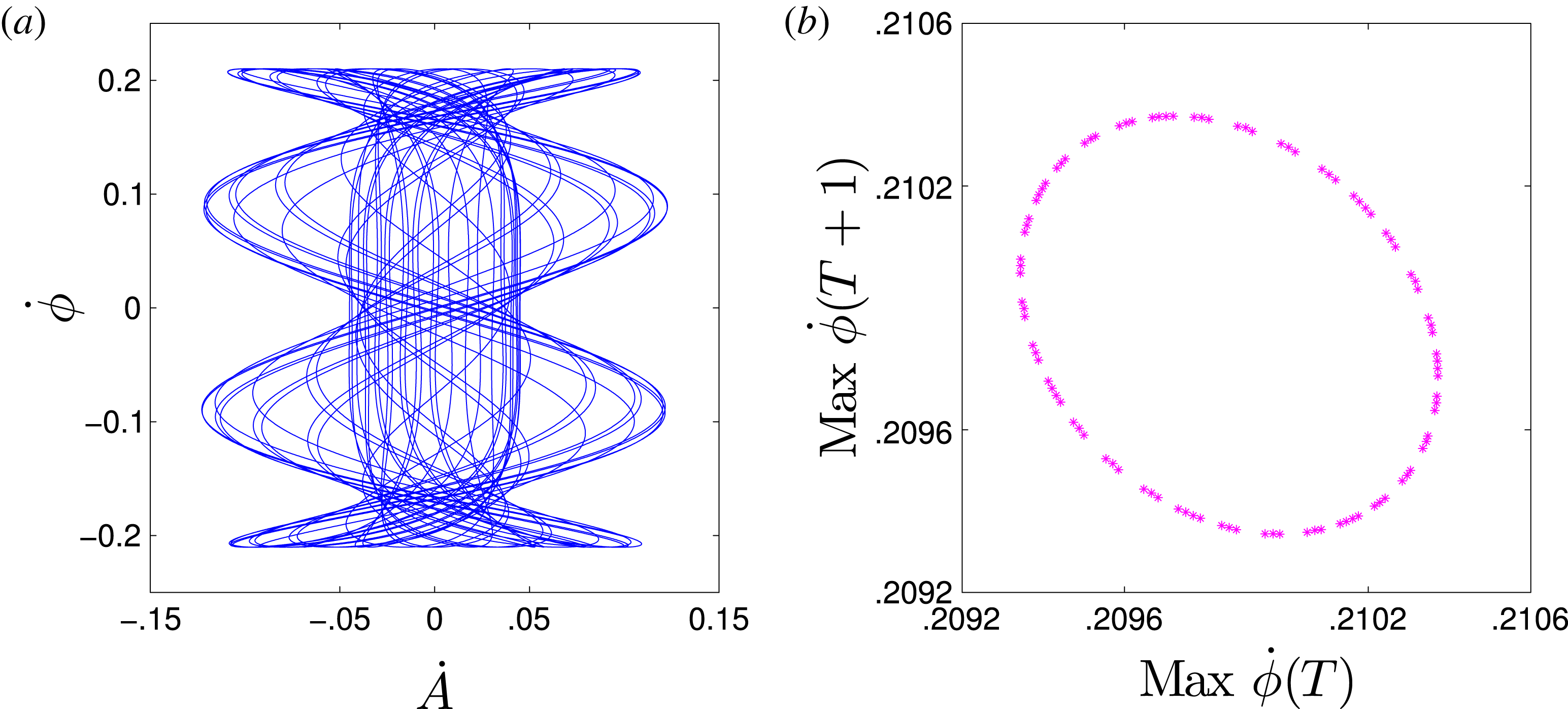
We have solved the system of differential equations (2.16)–(2.19) numerically with ${\it\alpha}=4.0$ , ${\it\beta}=1.01$ , and $H=0.2$ , and corresponding phase diagrams as well as Poincaré sections are shown for different values of $M$ in phase plane ${\dot{A}}{-}\dot{{\it\phi}}$ in figures 3 and 4. The technique of Poincaré surface section diagrams has been very helpful in studying qualitative properties of a dynamical system, as it allows one to trace the properties of periodic and quasi-periodic orbits of the original higher-dimensional system, as projected on a lower-dimensional space (Poincaré surface). In the Poincaré map, an unstable periodic orbit turns into a set of saddle points with their associated stable and unstable manifolds. The stable manifold is a curve in the phase space on which each initial condition converges to a saddle point in forward time dynamics. The unstable manifold is a curve whose points converge to a saddle point in the time-reversed dynamics (Alligood, Sauer & Yorke Reference Alligood, Sauer and Yorke1996). Most initial conditions in the close vicinity of a saddle point are repelled from it.

Figure 3.

(a) Phase portrait and (b) Poincaré section of the given system for $M=9.0$ with ${\it\alpha}=4.0$ , ${\it\beta}=1.01$ , and $H=0.2$ .

We have plotted the phase portrait and Poincaré map of the system for $M=9.0$ in figure 3. The existence of quasi-periodic behaviour is clear from the return map of $\dot{{\it\phi}}$ in figure 3 for $M=9.0$ . A quasi-periodic motion of a system is composed of incommensurable periodic motions and the trajectory in phase space winds around on a torus filling its surface densely. The return map data lie on smooth closed curves, confirming the existence of quasi-periodic behaviour of the system for $M=9.0$ . In figure 4 the phase diagram and Poincaré map of the system are presented for $M=2.0$ . The irregular set of points in the whole Poincaré plane guarantees the existence of chaos in the system for $M=2.0$ . Chaos is aperiodic long-term behaviour of a system which has sensitive dependence on initial conditions. In the presence of chaos a small change in initial conditions causes unpredictable variation of oscillation pattern of the state variables. Therefore state variables have unpredictable bounded oscillation in the phase space for a chaotic system. We observe quasi-periodic and chaotic behaviour of the system for different values of $M$ .

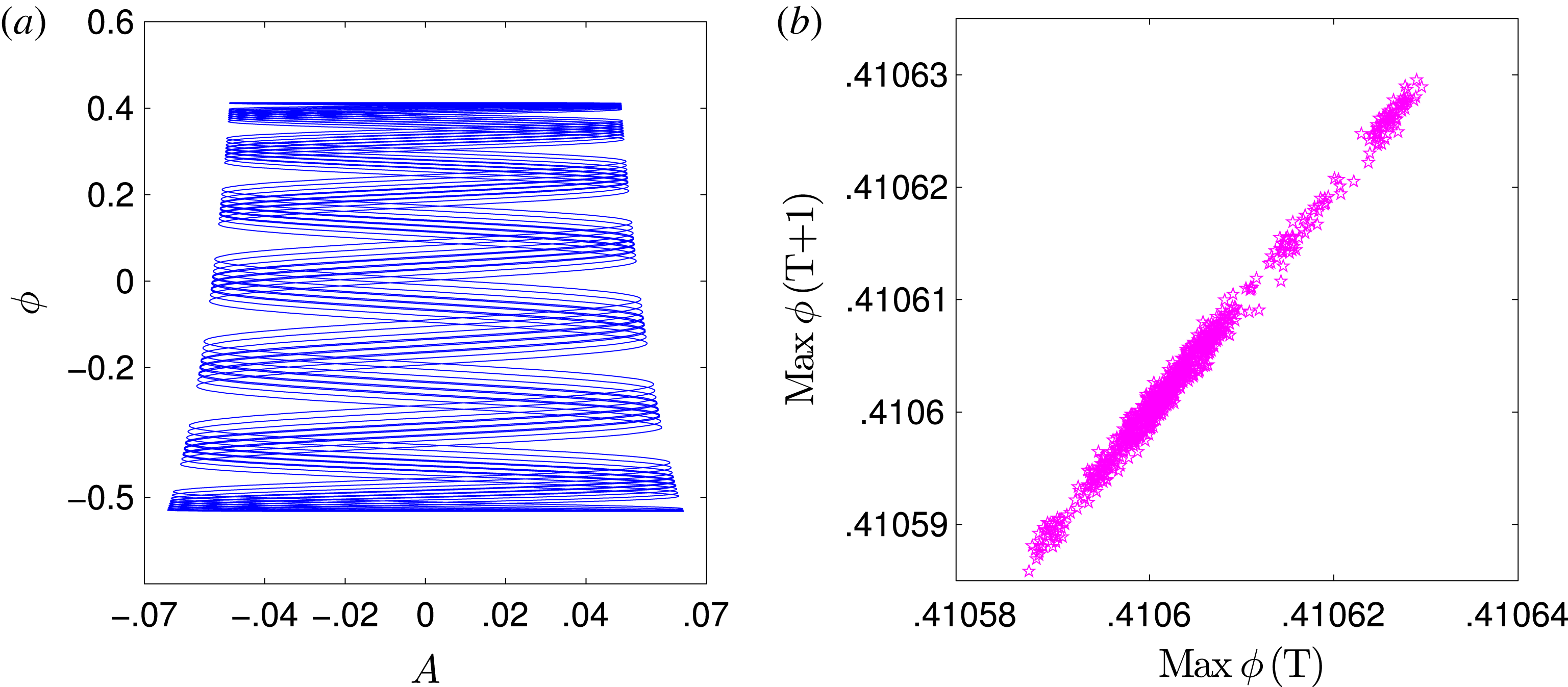
The phase diagram and Poincaré map of the system with ${\it\alpha}=4.0$ , ${\it\beta}=1.01$ , $M=5.0$ and for different $H$ , in the ${\it\phi}{-}A$ plane, are shown in figure 5 and figure 6. The phase diagram and corresponding Poincaré section for $H=0.2$ are presented in figure 5. The quasi-periodic behaviour of the system is clear from the Poincaré section. The phase diagram of the system and corresponding Poincaré section are depicted in figure 6 for $H=0.02$ . The Poincaré section confirms the existence of chaos in the system. It is also observed from numerical analysis that the dynamical behaviour does not change significantly due to variation of ${\it\beta}$ . Therefore, quasi-periodic as well as chaotic oscillations are possible in the present plasma system with the variation of Mach number and quantum parameter.

Figure 4.

(a) Phase portrait and (b) Poincaré section of the given system for $M=2.0$ with ${\it\alpha}=4.0$ , ${\it\beta}=1.01$ , and $H=0.2$ .

Figure 5.

(a) Phase portrait and (b) Poincaré section of the given system for $H=0.2$ with ${\it\alpha}=4.0$ , ${\it\beta}=1.01$ , and $M=5.0$ .

Figure 6.

(a) Phase portrait and (b) Poincaré section of the given system for $H=0.02$ with ${\it\alpha}=4.0$ , ${\it\beta}=1.01$ , and $M=5.0$ .