Introduction

Drifting snow is an important topic in both the engineering and climatological fields. Although recent research has revealed many basic properties of drifting snow, the time needed to reach steady-state conditions, including not only the saltation but also suspension, remains controversial. This is due to a lack of observational data, and the difficulty of expressing the transition between saltation and suspension using the majority of the current mathematical models.

In this study, the time evolution of drifting snow under a steady wind with turbulence was estimated using a numerical model. In the model, Lagrangian stochastic theory is used to incorporate the effect of turbulence on the motion of drifting-snow particles (Reference Sato, Uematsu and KanedaSato and others, 1997; Reference Sundsbø and HansenSundsbø and Hansen, 1997;Reference Taylor, Li and WilsonTaylor and others, 2002).This method enables us to discuss both the saltation and the suspension process. Aerodynamic entrainment, grain/bed collision (splash process), wind modification, and particle size distribution, according to the self-regulatory saltation model of sand (Reference Anderson and HaffAnderson and Haff, 1988, Reference Anderson and Haff1991;Reference McEwan and WillettsMcEwan and Willetts, 1991, Reference McEwan and Willetts1993), are also taken into account. The calculated time-scale results will be discussed in conjunction with the development of a spatial length scale of drifting snow, and will be compared with results reported in other studies on the spatial development of drifting snow.

Numerical Model

The model used in this study is one-dimensional and time-dependent. It calculates each particle trajectory under a steady wind with turbulent fluctuation over a flat, uniform snow surface. Although this approach requires large computational loads and cannot be applied to large areas (Reference GauerGauer, 2001), it is physically more sound than other methods and is useful for exploring the basic dynamics of drifting snow.

Furthermore, the model includes four distinct sub-processes (aerodynamic entrainment, the trajectory of the grains, splash process and the wind velocity modification) which are essential for aeolian sediment transport.

Particle trajectories are calculated within a small domain over a flat surface with periodic boundary conditions, under a horizontally uniform wind (Fig. 1). In the domain, snow particles start to move from random positions on the bed, owing to the aerodynamic entrainment. The number of entrained grains is calculated at each time-step.When a particle collides with the surface, the number, the velocities and the size of ejected grains are determined by splash functions. Thermodynamic effects (sublimation of the snow particles, humidity, temperature, etc.) are not taken into consideration; specific attention is paid to the grain dynamics in this study. The particles passing the end of the grid at a given height were counted in order to estimate the vertical distribution of the streamwise mass flux. The wind modification owing to the momentum exchange between the grains and the wind is also calculated at each vertical grid.

Fig. 1.

Schematic diagram of the calculation configuration. A periodic boundary condition was applied for the trajectory calculation (dashed line).

Within the atmospheric surface layer over a plane, the mean wind velocity is typically large with respect to the horizontal wind fluctuation, and the mean vertical wind is zero. Therefore, in the two-dimensional case, the wind velocity vector u can be approximated by u = (U;w′), where U is the mean wind speed and w′ the vertical wind fluctuation. Themeanwind field follows the Reynolds-averaged Navier–Stokes equation for a steady state (@/@t = 0) and horizontal homogeneity (@/@x = 0). Using Prandtl’s mixing length theory, we obtain the horizontal momentum equation for air

where ρ_f is the density of air, and κ the von Kármán constant. The coupling force F_x corresponds to the rate of the time change of particle momentum as

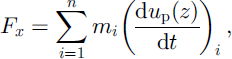
where n is the total number of particles per unit volume at height z;mthe particle mass, and (du_p(z)/dt) the horizontal acceleration of a particle at height z above the surface.

w′ is determined by the random-flight model (e.g.Reference Wilson and SawfordWilson and Sawford, 1996). For a fluid parcel i, w′_i at time t þ Δt is expressed as

where Δt is a time increment, σ_w is the standard deviation of the vertical wind, ξ is a Gaussian random variable with zero mean and unit variance and T_L is the Lagrangian time-scale. In the surface layer, T_L can be expressed in terms of friction velocity u* and height above the surface z as T_L = 0.4z/u* (Reference Wilson and SawfordWilson and Sawford, 1996). Lagrangian tracking techniques are suitable for turbulent particle dispersion, and a similar method has been applied to the simulation of blowing- and drifting-snow particles emitted from a fixed point, by Reference Sato, Uematsu and KanedaSato and others (1997), Reference Sundsbø and HansenSundsbø and Hansen (1997) and Reference Taylor, Li and WilsonTaylor and others (2002).

In the calculation of particle trajectories, we should obtain the vertical wind fluctuation w0_pi at each particle’s position, which is strictly different from w′_i because of the particle inertia and gravitational settling (crossing-trajectories effect). Reference Hunt and NalpanisHunt and Nalpanis (1985) modeled the vertical fluid velocity seen by a solid particle using Equation (3), but with a Lagrangian time-scale,

where A₁ is a constant of O(1). In this study, we use Equation (4) as the Lagrangian time-scale. A₁ is set to 0.5 according to Reference AndersonAnderson (1987).

The grain-borne shear stress τ_g is calculated from the particle trajectories as

where n↓ and n↑ show the particle number per unit area in unit time (the vertical number flux density of particles) on moving upward and downward, respectively. u_pi↑ and u_pi↓ are the horizontal speed of the ith particle moving upward and downward, respectively.

Motion of the particles is mainly determined by two forces: gravitational force and drag force due to the wind (Reference Nishimura and HuntNishimura and Hunt, 2000; Reference GauerGauer, 2001). Assuming the particle shape is spherical, the equation of motion for a snow particle is

where g is the gravitational acceleration, d the particle diameter, and u_p and u are particle and wind velocity, respectively. C_d is the drag coefficient, which is determined according to Reference Morsi and AlexanderMorsi and Alexander (1972). V_R is the relative velocity between a particle and the wind, defined as

Particle trajectories are determined by Equation (6) provided the initial conditions and the wind field are known. To provide initial conditions for the particles, aerodynamic entrainment and splash processes are considered. The process of aerodynamic entrainment is modeled based on the excess shear stress rule, which was first proposed by Anderson and Haff (Reference Anderson and Haff1988, Reference Anderson and Haff1991). In regard to the splash process, experimentally determined splash functions expressing the probability distributions of the vertical restitution coefficient, horizontal restitution coefficient and ejection number, formulated by Reference Sugiura and MaenoSugiura and Maeno (2000), are used. Their experiment was conducted in a cold wind tunnel (–15°C) with natural compacted snow. The snow particles on the surface were not sintered. Hence, our model simulations are also restricted over the loose snow. In addition, functions are obtained at relatively low wind speed. Since the splash process can be drastically modified by the strong turbulence at higher wind speeds (Reference Nishimura and HuntNishimura and Hunt, 2000), Sugiura and Maeno’s splash functions would be applicable only at moderate wind (say 5–10ms^–1 at height 1 m).The particle diameters at the lower boundary were given with a gamma random number distribution, according to the previous observations (e.g. Reference BuddBudd, 1966).

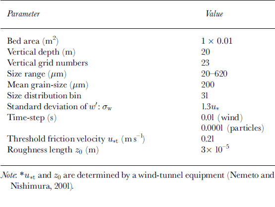
Table 1 and Table 2 show the list of the model parameters and the initial and lower boundary conditions for the wind field, respectively. In Table 1, the threshold friction velocity of drifting snow u*_t and the roughness length over the snow surface z₀ are determined by a wind-tunnel experiment (Reference Nemoto and NishimuraNemoto and Nishimura, 2001). In the simulation, we use two time-steps, 10^–2s and 10^–4 s; the latter is for the grain trajectory calculation and is two orders of magnitude smaller than the former for wind calculation, in order to adequately resolve each grain trajectory. The vertical dimension is discretized into slices, and within each slice the wind speed is calculated by the balance of the body force due to the grains and the wind shear stress (Reference McEwan and WillettsMcEwan and Willetts, 1991, Reference McEwan and Willetts1993). Detailed descriptions of the model and calculation procedures have been provided in Reference NemotoNemoto (2002) and will be published separately.

Table 1.

List of the model parameters

Table 2.

Initial and lower boundary conditions for the wind field

Results

Discussion and Conclusions

In this study, we have shown results of time-series data obtained by a new numerical model of drifting snow. The basic concept of the model is the same as that of the self-regulating saltation model for sand (Reference Anderson and HaffAnderson and Haff, 1988, Reference Anderson and Haff1991; Reference McEwan and WillettsMcEwan and Willetts, 1991, Reference McEwan and Willetts1993). In addition, the effect of vertical turbulent wind on the particle trajectories is incorporated. Hence, the model can represent the mass-flux development within both the saltation layer and the suspension layer.

In the cases examined (u_*i = 0.32 and 0.39ms^–1), the time it takes for the total mass flux to reach a steady state appears to be 3–5 s. Vertical profiles of horizontal mass flux near the surface (i.e. in the saltation layer) show a similar tendency. In contrast, for the wind structure and the whole mass-flux profile, it takes >50 s to reach a steady state. This longer duration is due to the relatively long time needed to reach the final mass-flux profile, which extends to an order of a few meters high due to turbulent diffusion. In the surface layer, the eddy diffusivity coefficient K_m can be expressed in terms of friction velocity and height above the surface as K_m = κu_*z. From this relation, we define a diffusion time-scale T(s) as

If we consider the case u_* = 0.32ms^–1, the thickness of the drifting-snowlayer z is approximately 10 mas shown in Figure 4. Therefore, from Equation (8), we obtain T ~ 78 s, which is of the same order as the calculated time. This consistency indicates that the turbulence has a significant effect on the dispersion and development of drifting snow.

Although the horizontal mass flux near the surface reaches saturation in the early stages of drifting snow, horizontal mass flux at z > 1m continues to increase at this stage and takes much longer to reach saturation. This result seems to contradict the fact that the total mass flux attains a steady state in a relatively short time. However, as shown in Figure 4, the mass flux in the suspension layer is more than three orders ofmagnitude smaller than the mass flux near the surface. Thus, no change is observed in the mass flux near the surface.

Time-series data of the wind speeds at u_*i = 0.32ms^–1 (Fig. 9) show that the wind structure also changes noticeably during approximately 50 s, particularly at high positions. Reference McEwan and WillettsMcEwan andWilletts (1993) reported that in their simulations it took >40 s for the boundary layer to respond to the development of sand saltation at u_*i = 0.32ms^–1. They considered that the increase in effective roughness, accompanied by the sand saltation, gave rise to the change in the wind structure at the surface and propagated upwards from there. Our results for the response time of the wind structure (~50 s) are similar to theirs, although the transition from saltation to suspension is included in our model. In the suspension layer, the momentum exchange between grains and the wind is small because the particle number flux is much smaller than it is in the saltation layer, and the particles have small mass (i.e. small diameter) and the relative velocity is small. The effect of particle inertia is presumably negligible in the suspension layer. Therefore, we can conclude that the wind modification obtained in our model is mainly induced by the saltating particles near the surface, which have large diameter and more inertia.

In this study, the time taken for the saltation and suspension layer of drifting and blowing snow to reach a steady state is found to be several tens of seconds, when the initial friction velocity u_* = 0.32 and 0.39ms^–1. However, some numerical models based on continuous theory (Reference Déry, Taylor and XiaoDéry and others, 1998; Reference MannMann, 1998; Reference BintanjaBintanja, 2000; Reference Xiao and TaylorXiao and Taylor, 2002) suggest a much longer time is needed, such as several tens of minutes (Reference Xiao, Bintanja, Déry, Mann and TaylorXiao and others, 2000). The discrepancy can be explained as follows. Our model incorporates the effect of turbulence on the motion of drifting-snow particles and describes both saltation and suspension processes. Thus the wind-speed modification (reduction) due to the momentum exchange between grains and the wind near the bed is also taken into account. It is important because it causes a sudden decrease in the wind near the surface (Fig. 9) and leads to the reduction of the ejection rate on the bed. On the other hand, much attention has been paid to suspension in other models; the saltation layer was given as a lower boundary condition. The wind modification above the saltation layer can be slower than it is in the saltation layer, which leads to a slow evolution of the system. The grain/bed collision process (splash function), which is omitted from other models, may affect the time-scale. It is also possible that the thermodynamic effect, which is not considered in our model (e.g. sublimation of the drifting-snow particles), lengthens the time required to achieve a steady state. As a next step, we will include the thermodynamics in our model to see how it affects the time-scale concerned.

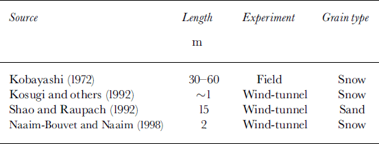
The spatial scale of the development of the saltation and suspension layer has remained a controversial issue because there are few examples of observation; Reference TakeuchiTakeuchi’s (1980) field observation may be the only one. The model used in this study calculates the time development of vertical distribution of the mass flux and the wind; fundamentally, it is a one-dimensional model. Although the approach is physically more sound than that of other models, it is difficult to apply a vast multidimensional area of calculation with this type of model because the number of particles in the calculation is limited, as already mentioned. However, despite this restriction, applying Taylor’s frozen turbulence approximation we can indirectly estimate the spatial scale of drifting-snow development. Considering a homogeneous field in a uniform mean wind, spatial changes in a turbulence variable and its temporal changes at a fixed point can be related to each other as ∂/∂t = -U∂/∂x, where U is the mean wind velocity. The time development of the horizontal mass-flux profile is shown in Figure 4. Applying Taylor’s hypothesis, we can closely relate the time development to the spatial development of the horizontal mass-flux profile in the mean wind direction. Given that the mean wind speed at 1 m height was approximately 8 ms^–1, the profiles in Figure 4 (t =0.6, 1.5, 2.5, 10, 30 and 50 s) can be considered to correspond to x = 4.8, 12.0, 20.0, 80.0, 240.0 and 400 m, respectively. Thus, we can reasonably say that the streamwise distance reaching the drifting-snow steady state is approximately 400 m.Reference TakeuchiTakeuchi (1980) observed the horizontal distribution of the total mass flux in drifting snow. His observation indicated that the total mass flux increased rapidly from the onset to 100–200m, and reached a steady state after around 200–400m for a wind speed at 1m height of 7– 8 ms^–1. The estimated length scale fromTaylor’s hypothesis shows good agreement. The length scale obviously depends on the wind speed. In fact, several observations have showed that drifting snow achieves a steady state within a shorter length scale when saltation is dominant (Table 3). This feature is successfully reproduced by our model. However, for the larger wind (say u_* > 1ms^–1), much improvement of the model will be necessary. In particular, the splash process, which can be a function not only of the friction velocity but also of the temperature and snow properties, is important for the development of drifting snow (see Reference Naaim-Bouvet and NaaimNaaim-Bouvet and Naaim, 1998). More investigation and model improvement will increase our understanding of the drifting- and blowing-snow process and will make it possible to estimate the transport rate under different conditions.

In this study, the horizontal wind U changes in time but is assumed to be uniform within a small domain. In reality, however, drifting snow develops in the mean wind direction, and the horizontal advection term (∂/∂x) would not be zero; U is a function of both time and space. Reference Shao and LiShao and Li (1999) reported a two-dimensional saltation model for sand. Their results indicate U(x) decreases with x from the starting point of saltation, and as far as the saltation layer is concerned, equilibrium saltation is achieved at a distance around 15 m, which corresponds to t < 1 s. The reduction of U in the mean wind direction would shorten the equilibrium time. The extension of our model to two dimensions is the logical next step to investigate precisely the time and length scale of drifting snow.

Table 3.

Observed distance for saltation layer to reach equilibrium