


1 Introduction
In recent decades, electrokinetic phenomena, such as electro-osmosis, streaming potential and streaming current, have attracted wide attention and application thanks to advances in micro- and nanofabrication technologies (Schoch, Han & Renaud Reference Schoch, Han and Renaud2008; Sparreboom, van den Berg & Eijkel Reference Sparreboom, van den Berg and Eijkel2010). In general, most solid surfaces obtain a surface electrical charge when they are in contact with a polarizable electrolyte solution. This surface charge leads to the formation of an electrical double layer (EDL) at the solid–liquid interface (Li Reference Li2004; Masliyah & Bhattacharjee Reference Masliyah and Bhattacharjee2006). The charged walls of a microchannel will become increasingly important in the nano-regime because of the larger surface-to-volume ratio (Stein, Kruithof & Dekker Reference Stein, Kruithof and Dekker2004; Bocquet & Charlaix Reference Bocquet and Charlaix2010). When pressure-driven transport ensues in a microchannel, the fluid flow drives the net charge within the EDL downstream, thereby resulting in an electric current, known as the streaming current. The accumulation of charges at the channel downstream creates an electric potential difference between the two ends of the channel, termed the streaming potential (Das, Guha & Mitra Reference Das, Guha and Mitra2013). The establishment of streaming current and streaming potential in microchannels provides the possibility of converting mechanical energy into electrical power, as reported by experimental and theoretical studies (Osterle Reference Osterle1964; Yang et al. Reference Yang, Lu, Kostiuk and Kwok2003; Olthuis et al. Reference Olthuis, Schippers, Eijkel and van den Berg2005; Daiguji et al. Reference Daiguji, Oka, Adachi and Shirono2006; Xuan & Li Reference Xuan and Li2006; Xie et al. Reference Xie, Wang, Xue, Jin, Chen and Wang2008; Chang & Yang Reference Chang and Yang2010, Reference Chang and Yang2011; Wang & Kang Reference Wang and Kang2010; Zhang et al. Reference Zhang, Wang, Yeh, Pan, Lin, Yu, Zhang, Zheng, Jiao and Wang2015). Especially, nanoscale fluidic devices allow the probing of the regime of EDL overlap, where the electrokinetic energy conversion efficiency is expected to be highest (Daiguji et al. Reference Daiguji, Yang, Szeri and Majumdar2004b ; van der Heyden et al. Reference van der Heyden, Bonthuis, Stein, Meyer and Dekker2006, Reference van der Heyden, Bonthuis, Stein, Meyer and Dekker2007; Pennathur, Eijkel & van den Berg Reference Pennathur, Eijkel and van den Berg2007; Siria et al. Reference Siria, Poncharal, Biance, Fulcrand, Blase, Purcell and Bocquet2013; Ding et al. Reference Ding, Jian, Wang and Yang2017).
For practical micro- or nanochannels filled with electrolyte solution, it is found that the electrical conductance of the Stern layer within the EDL reduces the efficiency and power output significantly (van der Heyden et al. Reference van der Heyden, Bonthuis, Stein, Meyer and Dekker2007; Davidson & Xuan Reference Davidson and Xuan2008a ). On the other hand, recent studies have shown that the energy conversion efficiency may be improved remarkably by employing, for example, velocity slip (Davidson & Xuan Reference Davidson and Xuan2008b ; Ren & Stein Reference Ren and Stein2008), soft nanochannels (Chanda, Sinha & Das Reference Chanda, Sinha and Das2014; Patwary, Chen & Das Reference Patwary, Chen and Das2016), steric effect (Bandopadhyay & Chakraborty Reference Bandopadhyay and Chakraborty2011), viscoelastic fluids (Bandopadhyay & Chakraborty Reference Bandopadhyay and Chakraborty2012; Jian et al. Reference Jian, Li, Liu, Chang, Liu and Yang2017), time-periodic pressure (Goswami & Chakraborty Reference Goswami and Chakraborty2010), polymer addition (Nguyen et al. Reference Nguyen, Xie, de Vreede, van den Berg and Eijkel2013), buffer anions effect (Mei, Yeh & Qian Reference Mei, Yeh and Qian2017), transverse magnetic fields (Munshi & Chakraborty Reference Munshi and Chakraborty2009) and layering of large ions near the wall–liquid interface (Gillespie Reference Gillespie2012). Liu et al. (Reference Liu, Ding, Mo, Chen, Yang, Li, Xie, Zhou and Zhou2016) presented a flexible microfluidics nanogenerator, which may offer an approach for building up self-powered systems by harvesting human mechanical energy. However, there exist two different approaches to evaluate efficiency in the literature. Some groups (e.g. Daiguji et al. Reference Daiguji, Oka, Adachi and Shirono2006; Xuan & Li Reference Xuan and Li2006; Davidson & Xuan Reference Davidson and Xuan2008b ; Chang & Yang Reference Chang and Yang2010) computed the output power and conversion efficiency based on thermodynamic analysis; while other groups (e.g. Yang et al. Reference Yang, Lu, Kostiuk and Kwok2003; van der Heyden et al. Reference van der Heyden, Bonthuis, Stein, Meyer and Dekker2006, Reference van der Heyden, Bonthuis, Stein, Meyer and Dekker2007; Gillespie Reference Gillespie2012) used electric circuit analysis. We will review and discuss them in the next section.
Recently, Xie et al. (Reference Xie, Sherwood, Shui, van den Berg and Eijkel2011) showed that injection of gas bubbles into a liquid-filled channel increases both the maximum output power and the energy conversion efficiency. In subsequent work (Sherwood et al. Reference Sherwood, Xie, van den Berg and Eijkel2013), they presented a theoretical analysis of the generation of streaming currents and electrical power by two-phase flow under various flow patterns in a rectangular microchannel where low wall zeta potential and thin EDL relative to the channel height have been assumed. In their research, the injection of a second, non-conducting fluid phase tends to decrease the effective cross-section of the channel, thereby decreasing the conduction current, which causes power dissipation and lowers efficiency. However, this mechanism may be invalid in nanochannels with a thick EDL because the reduction in effective cross-section also leads to a decrease in streaming current.
In nanofluidic channels, the electrostatic properties at the liquid–liquid interface may have a significant effect on electrokinetic energy conversion. In this paper, we focus on the performance of nanofluidic energy conversion systems using a model of two-layer fluid flow where the effects of electrostatic properties at the liquid–liquid interface are investigated in detail. On the other hand, in order to examine the energy transfer among different forms in electrokinetic flows, we derive the mechanical energy equation by combining thermodynamic and fluid mechanics on the system.
In a two-layer fluid system consisting of two immiscible electrolytes, an EDL is also formed at the liquid–liquid interface (Choi et al. Reference Choi, Sharma, Qian, Lim and Joo2011; Gopmandal & Ohshima Reference Gopmandal and Ohshima2017; Saha, Gopmandal & Ohshima Reference Saha, Gopmandal and Ohshima2017). However, a key difference is the presence of mobile ions along the liquid–liquid interface (Lee & Li Reference Lee and Li2006; Movahed et al. Reference Movahed, Khani, Wen and Li2012). In addition, Volkov et al. (Reference Volkov, Deamer, Tanelian and Markin1996) have pointed out that, at the interface of two immiscible electrolyte solutions, a narrow region exists where the electric potential changes abruptly due to the adsorption of ions. The sharp change at this layer can often be described by a zeta potential jump across the interface (Choi et al. Reference Choi, Sharma, Qian, Lim and Joo2011; Su et al. Reference Su, Jian, Chang and Li2013; Jian et al. Reference Jian, Su, Chang, Liu and He2014; Shit et al. Reference Shit, Mondal, Sinha and Kundu2016). Therefore, for practical purposes, the surface charge and zeta potential jump are incorporated to describe the boundary condition at the interface. Furthermore, semi-analytical expressions for the velocity, output power and energy transfer efficiency for the two-fluid system are obtained by considering large wall potentials, and the finite conductance of the Stern layer.
This paper is organized as follows. In § 2 we review the general framework for electrokinetic energy conversion in micro- and nanofluidic channels. The physical description of a two-fluid system and the solution to the equations governing the distributions of EDL potential and velocity in two-layer fluids are presented in § 3. We examine in § 4 the performance of practical electrokinetic energy converters. A summary of our results is provided in § 5.
2 General framework for electrokinetic energy conversion
As stated in the introduction, when the flow is driven by a pressure gradient, a streaming current and streaming potential can be established and pressure-to-voltage energy conversion can be achieved. Within the linear response regime of electrokinetic flows, the electric current and flow rate through a micro/nanochannel are often described well by the Onsager reciprocal relation (Brunet & Ajdari Reference Brunet and Ajdari2004; van der Heyden et al. Reference van der Heyden, Bonthuis, Stein, Meyer and Dekker2006; Xuan & Li Reference Xuan and Li2006)
 $$\begin{eqnarray}\displaystyle & \displaystyle Q=L_{11}(-\unicode[STIX]{x0394}p)+L_{12}(-\unicode[STIX]{x0394}\unicode[STIX]{x1D719}), & \displaystyle\end{eqnarray}$$
 $$\begin{eqnarray}\displaystyle & \displaystyle I=L_{21}(-\unicode[STIX]{x0394}p)+L_{22}(-\unicode[STIX]{x0394}\unicode[STIX]{x1D719}), & \displaystyle\end{eqnarray}$$
where
 $L_{11}$
represents the hydrodynamic conductance of the channel,
 $L_{12}=L_{21}$
characterizes the streaming conductance,
 $L_{22}$
indicates the electrical conductance of the channel, and
 $\unicode[STIX]{x0394}p$
and
 $\unicode[STIX]{x0394}\unicode[STIX]{x1D719}$
are the pressure difference and the electric potential difference between the channel ends, respectively. The conductance tensor
 $\unicode[STIX]{x1D647}=(\unicode[STIX]{x1D613}_{ij})$
must be positive definite by the second law of thermodynamics (Prigogine Reference Prigogine1968). In (2.2), the term
 $L_{21}(-\unicode[STIX]{x0394}p)$
is the so-called streaming current (denoted by
 $I_{s}$
), while
 $L_{22}(-\unicode[STIX]{x0394}\unicode[STIX]{x1D719})$
is the conduction current
 $(I_{c})$
. Furthermore, the zero-current condition (i.e.
 $I=0$
) leads to an open-circuit voltage, namely, the streaming potential
 $\unicode[STIX]{x0394}\unicode[STIX]{x1D719}_{s}=L_{21}(-\unicode[STIX]{x0394}p)/L_{22}$
. It should be noted that the linear Onsager reciprocal relation will fail when the non-equilibrium concentration polarization phenomenon occurs at the two ends of a channel (Chang & Yang Reference Chang and Yang2010, Reference Chang and Yang2011).
In the literature, the electrokinetic energy conversion efficiency has been calculated in different ways. For example, Xuan & Li (Reference Xuan and Li2006) calculate the maximum conversion efficiency based on thermodynamics while the work of van der Heyden et al. (Reference van der Heyden, Bonthuis, Stein, Meyer and Dekker2006) is based on the equivalent circuit. We compare these two ways in the following.
2.1 Thermodynamic analysis
The generation power
 $W$
and conversion efficiency
 $\unicode[STIX]{x1D709}$
can be written as
 $$\begin{eqnarray}W=I\unicode[STIX]{x0394}\unicode[STIX]{x1D719}\quad \text{and}\quad \unicode[STIX]{x1D709}=\frac{I\unicode[STIX]{x0394}\unicode[STIX]{x1D719}}{Q(-\unicode[STIX]{x0394}p)}.\end{eqnarray}$$
The generation power is maximized by
 $\unicode[STIX]{x0394}\unicode[STIX]{x1D719}=-\unicode[STIX]{x0394}pL_{12}/2L_{22}$
, which is exactly half of the streaming potential. The maximum generation power and the corresponding conversion efficiency are given by (Xuan & Li Reference Xuan and Li2006)
 $$\begin{eqnarray}W_{max\,W}=\frac{I_{s}\unicode[STIX]{x0394}\unicode[STIX]{x1D719}_{s}}{4}=\frac{\unicode[STIX]{x1D6FC}}{4}L_{11}(\unicode[STIX]{x0394}p)^{2}\quad \text{and}\quad \unicode[STIX]{x1D709}_{max\,W}=\frac{I_{s}\unicode[STIX]{x0394}\unicode[STIX]{x1D719}_{s}}{4Q(-\unicode[STIX]{x0394}p)}=\frac{\unicode[STIX]{x1D6FC}}{2(2-\unicode[STIX]{x1D6FC})},\end{eqnarray}$$
where the subscript
 $max\,W$
indicates the condition of maximum generation power,
 $\unicode[STIX]{x1D6FC}=L_{12}L_{21}/L_{11}L_{22}$
is the figure of merit for electrokinetic energy conversion, and
 $0\leqslant \unicode[STIX]{x1D6FC}<1$
due to the positive definiteness of
 $\unicode[STIX]{x1D647}$
. On the other hand, when the voltage satisfies
 $\unicode[STIX]{x0394}\unicode[STIX]{x1D719}=-\unicode[STIX]{x0394}p(1-\sqrt{1-\unicode[STIX]{x1D6FC}})L_{11}/L_{12}$
, the conversion efficiency is maximized. At this condition, the generation power and efficiency are given by (Xuan & Li Reference Xuan and Li2006)
 $$\begin{eqnarray}W_{max\,\unicode[STIX]{x1D709}}=L_{11}\frac{\sqrt{1-\unicode[STIX]{x1D6FC}}(1-\sqrt{1-\unicode[STIX]{x1D6FC}})^{2}}{\unicode[STIX]{x1D6FC}}(\unicode[STIX]{x0394}p)^{2}\quad \text{and}\quad \unicode[STIX]{x1D709}_{max\,\unicode[STIX]{x1D709}}=\frac{(1-\sqrt{1-\unicode[STIX]{x1D6FC}})^{2}}{\unicode[STIX]{x1D6FC}},\end{eqnarray}$$
where the subscript
 $max$
indicates the condition of maximum generation efficiency.
2.2 Electric circuit analysis
Consider such a fluidic device connected to an electrical resistor (with resistance
 $R_{L}$
) in a circuit (see figure 1
b). The efficiency is defined as the electrical power,
 $\unicode[STIX]{x0394}\unicode[STIX]{x1D719}^{2}/R_{L}$
, consumed by the load divided by the input mechanical pumping power,
 $Q(-\unicode[STIX]{x0394}p)$
. It is convenient to define a rescaled load resistance,
 $\unicode[STIX]{x1D6FA}=R_{L}/R_{ch}$
, relative to the channel resistance,
 $R_{ch}=1/L_{22}$
. The maximum electrical power can be achieved at
 $\unicode[STIX]{x1D6FA}=1$
. At this condition, the maximum power and the corresponding conversion efficiency are the same as in (2.4). Furthermore, the optimal efficiency and the corresponding generation power are found to be
 $$\begin{eqnarray}W_{max\,\unicode[STIX]{x1D709}}=L_{11}\frac{\sqrt{1-\unicode[STIX]{x1D6FC}}(1-\sqrt{1-\unicode[STIX]{x1D6FC}})^{2}}{\unicode[STIX]{x1D6FC}}(\unicode[STIX]{x0394}p)^{2}\quad \text{and}\quad \unicode[STIX]{x1D709}_{max\,\unicode[STIX]{x1D709}}=\frac{\unicode[STIX]{x1D6FC}}{\unicode[STIX]{x1D6FC}+2(\sqrt{1-\unicode[STIX]{x1D6FC}}+1-\unicode[STIX]{x1D6FC})},\end{eqnarray}$$
for
 $\unicode[STIX]{x1D6FA}=1/\sqrt{1-\unicode[STIX]{x1D6FC}}$
(van der Heyden et al.
Reference van der Heyden, Bonthuis, Stein, Meyer and Dekker2006). It is easy to verify that the efficiencies in (2.5) and (2.6) are the same, although they are in different forms.
(a) Schematic illustration of electrokinetic energy conversion in a nanochannel filled with two-layer fluids. A positive external pressure gradient
 $-\unicode[STIX]{x0394}p/l=-(p_{out}-p_{in})/l$
is applied across the nanochannel in the
 $x$
-direction, which drives the flow of mobile ions and thus induces a streaming current
 $I_{s}$
and a streaming electric field of strength
 $E_{s}=-\unicode[STIX]{x0394}\unicode[STIX]{x1D719}/l=-(\unicode[STIX]{x1D6F7}_{out}-\unicode[STIX]{x1D6F7}_{in})/l$
. This electric field, in turn, generates a current (conduction current
 $I_{c}$
) to flow back against the direction of the pressure-driven flow. (b) Equivalent electric circuit of the considered system connected to an external load resistor with adjustable resistance
 $R_{L}$
.

Interestingly, we find that the results (i.e. the electrical power and efficiency under the conditions of maximum output power and/or maximum efficiency) are the same whether based on thermodynamic or electric circuit analyses. Table 1 summarizes the electrical powers and conversion efficiencies obtained in different ways.
Summary of electrical power and conversion efficiency under the maximum power generation and/or maximum conversion efficiency conditions, based on thermodynamic and electric circuit analyses, respectively.

a Indicates the condition of maximum power generation.
b
Indicates the condition of maximum conversion efficiency, and the approximation is for small
 $\unicode[STIX]{x1D6FC}$
.
Comparing the two generation powers
 $W_{max\,W}$
and
 $W_{max\,\unicode[STIX]{x1D709}}$
in (2.4) and (2.5), we find that they are identical up to
 $O(\unicode[STIX]{x1D6FC}^{2})$
for small
 $\unicode[STIX]{x1D6FC}$
by means of
 $$\begin{eqnarray}\frac{\sqrt{1-\unicode[STIX]{x1D6FC}}(1-\sqrt{1-\unicode[STIX]{x1D6FC}})^{2}}{\unicode[STIX]{x1D6FC}}=\frac{\unicode[STIX]{x1D6FC}}{4}-\frac{\unicode[STIX]{x1D6FC}^{3}}{64}+O(\unicode[STIX]{x1D6FC}^{4}).\end{eqnarray}$$
Similarly, the two conversion efficiencies
 $\unicode[STIX]{x1D709}_{max\,W}$
and
 $\unicode[STIX]{x1D709}_{max\,\unicode[STIX]{x1D709}}$
are identical up to
 $O(\unicode[STIX]{x1D6FC}^{2})$
by means of
 $$\begin{eqnarray}\displaystyle & \displaystyle \frac{(1-\sqrt{1-\unicode[STIX]{x1D6FC}})^{2}}{\unicode[STIX]{x1D6FC}}=\frac{\unicode[STIX]{x1D6FC}}{4}+\frac{\unicode[STIX]{x1D6FC}^{2}}{8}+\frac{5\unicode[STIX]{x1D6FC}^{3}}{64}+O(\unicode[STIX]{x1D6FC}^{4}), & \displaystyle\end{eqnarray}$$
 $$\begin{eqnarray}\displaystyle & \displaystyle \frac{\unicode[STIX]{x1D6FC}}{2(2-\unicode[STIX]{x1D6FC})}=\frac{\unicode[STIX]{x1D6FC}}{4}+\frac{\unicode[STIX]{x1D6FC}^{2}}{8}+\frac{\unicode[STIX]{x1D6FC}^{3}}{16}+O(\unicode[STIX]{x1D6FC}^{4}). & \displaystyle\end{eqnarray}$$
Note that the upper bound of
 $\unicode[STIX]{x1D709}_{max\,W}$
is
 $1/2$
while the upper bound of
 $\unicode[STIX]{x1D709}_{max\,\unicode[STIX]{x1D709}}$
is 1. However, for typical electrokinetic energy converters, the value of
 $\unicode[STIX]{x1D6FC}$
is small (e.g.
 $\unicode[STIX]{x1D6FC}<0.5$
), so the above two extreme powers (or efficiencies) are essentially close to each other (Xuan & Li Reference Xuan and Li2006).
A few researchers (e.g. Daiguji et al.
Reference Daiguji, Yang, Szeri and Majumdar2004b
; Olthuis et al.
Reference Olthuis, Schippers, Eijkel and van den Berg2005; Berli Reference Berli2010; Chanda et al.
Reference Chanda, Sinha and Das2014) calculated the input volume flow rate
 $Q$
in the definition of the efficiency
 $\unicode[STIX]{x1D709}$
as the purely pressure-driven volume flow rate, i.e.
 $Q=L_{11}(-\unicode[STIX]{x0394}p)$
. In this situation, the maximum efficiency that can be achieved is
 $$\begin{eqnarray}\unicode[STIX]{x1D709}_{max}=\frac{I_{s}\unicode[STIX]{x0394}\unicode[STIX]{x1D719}_{s}}{4L_{11}(\unicode[STIX]{x0394}p)^{2}}=\frac{\unicode[STIX]{x1D6FC}}{4}.\end{eqnarray}$$
It is easy to see that the efficiency
 $\unicode[STIX]{x1D709}_{max}$
is the leading term of the above efficiency
 $\unicode[STIX]{x1D709}_{max\,W}$
or
 $\unicode[STIX]{x1D709}_{max\,\unicode[STIX]{x1D709}}$
by using (2.8) and (2.9). For small
 $\unicode[STIX]{x1D6FC}$
, these extreme efficiencies achieved under three different conditions are nearly identical, i.e.
 $\unicode[STIX]{x1D709}_{max}\approx \unicode[STIX]{x1D709}_{max\,W}\approx \unicode[STIX]{x1D709}_{max\,\unicode[STIX]{x1D709}}$
.
3 Two-fluid energy converter
We consider a steady unidirectional flow of two immiscible viscous fluids of constant viscosity
 $\unicode[STIX]{x1D707}_{i}$
, electrical permittivity
 $\unicode[STIX]{x1D700}_{i}$
and thickness
 $h_{i}$
confined between two micro parallel plates at distance
 $h~(=h_{1}+h_{2})$
, where
 $i=1$
and
 $2$
are associated with the upper (fluid 1) and the lower layer (fluid 2), respectively. The channel walls are considered to bear a negative surface charge. We assume the width
 $w$
and the length
 $l$
of the parallel plates are much larger than the height, i.e.
 $l,w\gg h$
, and the interface between these two immiscible fluids is planar. A two-dimensional coordinate system
 $(x,y)$
is established at the fluid–fluid interface, where the
 $x$
-axis is tangential to the plate surface and the
 $y$
-axis is perpendicular to the plate surface, as sketched in figure 1(a). We note that this model makes several simplifying assumptions by focusing entirely on the properties of the slit-like channel. For example, it ignores the entrance effects where the channel meets the reservoirs, and takes the potential drop between the electrode and the electrolyte to be zero.
3.1 Electrical double-layer electric potential distribution
We assume that the fluids contain binary symmetric electrolyte ions with valence
 $z_{+}=-z_{-}=z$
. Owing to the interaction between the electrolyte ions and the charged walls as well as the liquid–liquid interface, EDLs are formed. In addition, in a two-fluid system, an unequal partitioning of micro-ions between the two liquid phases is induced by the difference in the dielectric constant (Ohshima et al.
Reference Ohshima, Nomura, Kamaya and Ueda1985; Leunissen et al.
Reference Leunissen, Zwanikken, Van Roij, Chaikin and Van Blaaderen2007; Gopmandal & Ohshima Reference Gopmandal and Ohshima2017; Saha et al.
Reference Saha, Gopmandal and Ohshima2017). Considering the ion partitioning effect, the Boltzmann distribution satisfied by the electrolyte ions can be written as
 $$\begin{eqnarray}\left.\begin{array}{@{}ll@{}}\displaystyle n_{\pm }=n_{\infty }\exp \left(\mp \frac{ez\unicode[STIX]{x1D713}}{k_{B}T}\right), & 0<y<h_{1},\\ \displaystyle n_{\pm }=b_{\pm }n_{\infty }\exp \left(\mp \frac{ez\unicode[STIX]{x1D713}}{k_{B}T}\right), & -h_{2}<y<0.\end{array}\right\}\end{eqnarray}$$
Here,
 $\unicode[STIX]{x1D713}$
is the EDL electric potential,
 $n_{\pm }$
are the concentrations of the electrolyte ions,
 $b_{\pm }$
are the ion partition coefficients of the electrolyte ions with
 $n_{\pm }(0-)=b_{\pm }n_{\pm }(0+)$
,
 $n_{\infty }$
is the bulk ionic concentration at
 $\unicode[STIX]{x1D713}=0$
,
 $e$
is the electronic charge,
 $k_{B}$
is the Boltzmann constant and
 $T$
is the absolute temperature.
The equilibrium electric potential
 $\unicode[STIX]{x1D713}$
relative to the bulk electrolyte and the local volumetric net charge density
 $\unicode[STIX]{x1D70C}_{e}=ez(n_{+}-n_{-})$
can be related through the Poisson equation as
 $$\begin{eqnarray}\unicode[STIX]{x1D6FB}^{2}\unicode[STIX]{x1D713}=-\frac{\unicode[STIX]{x1D70C}_{e}}{\unicode[STIX]{x1D700}_{i}},\quad i=1,2.\end{eqnarray}$$
For the fully developed flow, the distribution of the electric potential can be regarded as a function of
 $y$
, i.e.
 $\unicode[STIX]{x1D713}=\unicode[STIX]{x1D713}(y)$
.
To solve the electric potential distributions within fluids 1 and 2, appropriate boundary conditions must be imposed. In previous studies, three different models have been adopted for the electrostatic properties of the surface: constant zeta potential (Yang et al.
Reference Yang, Lu, Kostiuk and Kwok2003; Davidson & Xuan Reference Davidson and Xuan2008a
,Reference Davidson and Xuan
b
), constant surface charge density (Daiguji, Yang & Majumdar Reference Daiguji, Yang and Majumdar2004a
; Daiguji et al.
Reference Daiguji, Yang, Szeri and Majumdar2004b
; Stein et al.
Reference Stein, Kruithof and Dekker2004; Chang & Yang Reference Chang and Yang2010) and local chemical equilibrium (Behrens & Grier Reference Behrens and Grier2001; van der Heyden et al.
Reference van der Heyden, Bonthuis, Stein, Meyer and Dekker2007; Wang & Kang Reference Wang and Kang2010). The surface charge essentially varies with the bulk ionic concentration, the pH value and the temperature of the solution, and the double-layer interactions. This implies that the chemical equilibrium model may be the most suitable one to describe the solid–liquid interface, compared with the other two models. But there are many parameters that need to be specified beforehand, such as the surface density
 $\unicode[STIX]{x1D6E4}$
of chargeable sites, pH value, equilibrium constant
 $p$
K describing the dissociation of SiOH groups and Stern layer phenomenological capacity
 $C$
(Behrens & Grier Reference Behrens and Grier2001). In order to avoid excessive complexity, the condition of constant surface charge density is used, which yields reasonable results and is much better than assuming a constant zeta potential (Stein et al.
Reference Stein, Kruithof and Dekker2004; van der Heyden, Stein & Dekker Reference van der Heyden, Stein and Dekker2005). Furthermore, the surface charges are related to the electric potential
 $\unicode[STIX]{x1D713}(y)$
through Gauss’ law:
 $$\begin{eqnarray}\unicode[STIX]{x1D70E}_{1}=\unicode[STIX]{x1D700}_{1}\left.\frac{\text{d}\unicode[STIX]{x1D713}}{\text{d}y}\right|_{y=h_{1}}\quad \text{and}\quad \unicode[STIX]{x1D70E}_{2}=-\unicode[STIX]{x1D700}_{2}\left.\frac{\text{d}\unicode[STIX]{x1D713}}{\text{d}y}\right|_{y=-h_{2}},\end{eqnarray}$$
where
 $\unicode[STIX]{x1D70E}_{1}$
and
 $\unicode[STIX]{x1D70E}_{2}$
are the surface charge densities of the upper plate and lower plate, respectively.
At the liquid–liquid interface
 $(y=0)$
, we impose the potential difference
 $\unicode[STIX]{x0394}\unicode[STIX]{x1D713}$
and Gauss’ law for the electrical displacement (Choi et al.
Reference Choi, Sharma, Qian, Lim and Joo2011; Jian et al.
Reference Jian, Su, Chang, Liu and He2014):
 $$\begin{eqnarray}\unicode[STIX]{x1D713}|_{y=0^{-}}-\unicode[STIX]{x1D713}|_{y=0^{+}}=\unicode[STIX]{x0394}\unicode[STIX]{x1D713}\quad \text{and}\quad \unicode[STIX]{x1D700}_{2}\left.\frac{\text{d}\unicode[STIX]{x1D713}}{\text{d}y}\right|_{y=0^{-}}-\unicode[STIX]{x1D700}_{1}\left.\frac{\text{d}\unicode[STIX]{x1D713}}{\text{d}y}\right|_{y=0^{+}}=\unicode[STIX]{x1D70E}_{s}.\end{eqnarray}$$
Here
 $\unicode[STIX]{x1D70E}_{s}$
denotes the interface charge density, which implies that the normal component of the electric displacement vector is discontinuous;
 $\unicode[STIX]{x0394}\unicode[STIX]{x1D713}$
and
 $\unicode[STIX]{x1D70E}_{s}$
are considered to be independent parameters (Choi et al.
Reference Choi, Sharma, Qian, Lim and Joo2011). In addition, the total charges in the channel can be expressed as
 $$\begin{eqnarray}Q_{c}=A\left(\int _{-h_{2}}^{h_{1}}\unicode[STIX]{x1D70C}_{e}\,\text{d}y+\unicode[STIX]{x1D70E}_{1}+\unicode[STIX]{x1D70E}_{2}+\unicode[STIX]{x1D70E}_{s}\right),\end{eqnarray}$$
where
 $A$
is the area of the plate. Substituting (3.3) into (3.4) yields
 $Q_{c}=0$
. This verifies the condition of electroneutrality in the channel.
We introduce the following non-dimensional variables:
 $$\begin{eqnarray}\left.\begin{array}{@{}c@{}}\displaystyle [Y,H_{1},H_{2}]=\frac{1}{h}[y,h_{1},h_{2}],\quad [\unicode[STIX]{x1D6F9},\unicode[STIX]{x0394}\unicode[STIX]{x1D6F9}]=\frac{ze}{k_{B}T}[\unicode[STIX]{x1D713},\unicode[STIX]{x0394}\unicode[STIX]{x1D713}],\\ \displaystyle [\overline{\unicode[STIX]{x1D70E}}_{1},\overline{\unicode[STIX]{x1D70E}}_{2},\overline{\unicode[STIX]{x1D70E}}_{s}]=\frac{zeh}{\unicode[STIX]{x1D700}_{1}k_{B}T}[\unicode[STIX]{x1D70E}_{1},\unicode[STIX]{x1D700}_{r}^{-1}\unicode[STIX]{x1D70E}_{2},\unicode[STIX]{x1D70E}_{s}],\end{array}\right\}\end{eqnarray}$$
and
 $K=h/\unicode[STIX]{x1D706}_{D}$
with the Debye screening length
 $\unicode[STIX]{x1D706}_{D}=\sqrt{\unicode[STIX]{x1D700}_{1}k_{B}T/2n_{\infty }z^{2}e^{2}}$
, where
 $\unicode[STIX]{x1D700}_{r}=\unicode[STIX]{x1D700}_{2}/\unicode[STIX]{x1D700}_{1}$
denotes the permittivity ratio. With these scaled variables, (3.1) and (3.2) reduce to
 $$\begin{eqnarray}\frac{\text{d}^{2}\unicode[STIX]{x1D6F9}}{\text{d}Y^{2}}=\left\{\begin{array}{@{}ll@{}}K^{2}\sinh \unicode[STIX]{x1D6F9}, & 0<Y<H_{1},\\ (2\unicode[STIX]{x1D700}_{r})^{-1}K^{2}[-b_{+}\exp (-\unicode[STIX]{x1D6F9})+b_{-}\exp \unicode[STIX]{x1D6F9}], & -H_{2}<Y<0.\end{array}\right.\end{eqnarray}$$
The corresponding dimensionless boundary conditions become
 $$\begin{eqnarray}\left.\begin{array}{@{}c@{}}\displaystyle \overline{\unicode[STIX]{x1D70E}}_{1}=\left.\frac{\text{d}\unicode[STIX]{x1D6F9}}{\text{d}Y}\right|_{Y=H_{1}},\quad \overline{\unicode[STIX]{x1D70E}}_{2}=-\left.\frac{\text{d}\unicode[STIX]{x1D6F9}}{\text{d}Y}\right|_{Y=-H_{2}},\quad \unicode[STIX]{x1D6F9}|_{Y=0^{-}}-\unicode[STIX]{x1D6F9}|_{Y=0^{+}}=\unicode[STIX]{x0394}\unicode[STIX]{x1D6F9},\\ \displaystyle \left.\unicode[STIX]{x1D700}_{r}\frac{\text{d}\unicode[STIX]{x1D6F9}}{\text{d}Y}\right|_{Y=0^{-}}-\left.\frac{\text{d}\unicode[STIX]{x1D6F9}}{\text{d}Y}\right|_{Y=0^{+}}=\overline{\unicode[STIX]{x1D70E}}_{s}.\end{array}\right\}\end{eqnarray}$$
Equation (3.6) with the boundary conditions (3.7) is solved iteratively through a second-order central difference scheme. The iteration procedure starts with a guessed value of the potential. Here we assume that the partition coefficients for cations and anions are identical, i.e.
 $b_{+}=b_{-}=b$
. The detailed scheme and algorithm can be found in appendix A. Meanwhile, the convergence and validity of the algorithm and the dependence of the results on the number of grid points are also analysed.
3.2 Flow field coupled with electrokinetic interaction
The flow maintained by constant pressure gradient
 $-\text{d}p/\text{d}x=-\unicode[STIX]{x0394}p/l$
is assumed to be one-dimensional, steady and fully developed; the body force is the electric field force
 $\unicode[STIX]{x1D70C}_{e}E_{s}=\unicode[STIX]{x1D70C}_{e}(-\unicode[STIX]{x0394}\unicode[STIX]{x1D719})/l$
. Thus in such a two-fluid system the governing equation for the velocity can be described by
 $$\begin{eqnarray}\unicode[STIX]{x1D707}_{i}\frac{\text{d}^{2}u}{\text{d}y^{2}}-\frac{\unicode[STIX]{x0394}p}{l}+\unicode[STIX]{x1D70C}_{e}E_{s}=0,\quad i=1,2,\end{eqnarray}$$
where
 $u(y)$
is the axial velocity along the positive
 $x$
-direction. At the solid–liquid interface, the no-slip conditions are given by
 $u|_{y=h_{1}}=u|_{y=-h_{2}}=0$
. The continuity of the velocity as well as the balance of the total stresses including the Maxwell stress and shear stress between the two layers should be applied at the liquid–liquid interface (Jian et al.
Reference Jian, Su, Chang, Liu and He2014)
 $$\begin{eqnarray}u|_{y=0^{+}}=u|_{y=0^{-}},\quad \left.\left(\unicode[STIX]{x1D707}_{1}\frac{\text{d}u}{\text{d}y}-\unicode[STIX]{x1D700}_{1}E_{s}\frac{\text{d}\unicode[STIX]{x1D713}}{\text{d}y}\right)\right|_{y=0^{+}}=\left.\left(\unicode[STIX]{x1D707}_{2}\frac{\text{d}u}{\text{d}y}-\unicode[STIX]{x1D700}_{2}E_{s}\frac{\text{d}\unicode[STIX]{x1D713}}{\text{d}y}\right)\right|_{y=0^{-}}.\end{eqnarray}$$
Combining the governing equations in different fluids with the related boundary conditions, the analytical solution of the velocity distribution can be derived as
 $$\begin{eqnarray}u=\left\{\begin{array}{@{}ll@{}}\displaystyle \frac{\unicode[STIX]{x0394}p}{2l\unicode[STIX]{x1D707}_{1}}[y^{2}-h_{1}^{2}+A_{2}(y-h_{1})]+\frac{\unicode[STIX]{x0394}\unicode[STIX]{x1D719}}{l\unicode[STIX]{x1D707}_{1}}[A_{1}(y-h_{1})+\unicode[STIX]{x1D700}_{1}(\unicode[STIX]{x1D713}_{1,w}-\unicode[STIX]{x1D713})], & 0\leqslant y\leqslant h_{1},\\ \displaystyle \frac{\unicode[STIX]{x0394}p}{2l\unicode[STIX]{x1D707}_{2}}[y^{2}-h_{2}^{2}+A_{2}(y+h_{2})]+\frac{\unicode[STIX]{x0394}\unicode[STIX]{x1D719}}{l\unicode[STIX]{x1D707}_{2}}[A_{1}(y+h_{2})+\unicode[STIX]{x1D700}_{2}(\unicode[STIX]{x1D713}_{2,w}-\unicode[STIX]{x1D713})], & -h_{2}\leqslant y\leqslant 0,\end{array}\right.\end{eqnarray}$$
where
 $$\begin{eqnarray}A_{1}=\frac{\unicode[STIX]{x1D707}_{r}\unicode[STIX]{x1D700}_{1}(\unicode[STIX]{x1D713}_{1,w}-\unicode[STIX]{x1D713}(0+))-\unicode[STIX]{x1D700}_{2}(\unicode[STIX]{x1D713}_{2,w}-\unicode[STIX]{x1D713}(0-))}{\unicode[STIX]{x1D707}_{r}h_{1}+h_{2}},\quad A_{2}=\frac{h_{2}^{2}-\unicode[STIX]{x1D707}_{r}h_{1}^{2}}{\unicode[STIX]{x1D707}_{r}h_{1}+h_{2}},\end{eqnarray}$$
 $\unicode[STIX]{x1D707}_{r}=\unicode[STIX]{x1D707}_{2}/\unicode[STIX]{x1D707}_{1}$
denotes the viscosity ratio, and
 $\unicode[STIX]{x1D713}_{1,w}$
and
 $\unicode[STIX]{x1D713}_{2,w}$
are the wall zeta potentials of the upper plate and lower plate, respectively.
Integrating the velocity (3.10) over the channel cross-section gives the volumetric flow rate
 $Q$
and then yields the expressions for the phenomenological coefficients in (2.1) as
 $$\begin{eqnarray}L_{11}=\frac{w}{2l}\left[\frac{2h_{1}^{3}}{3\unicode[STIX]{x1D707}_{1}}+\frac{2h_{2}^{3}}{3\unicode[STIX]{x1D707}_{2}}+A_{2}\left(\frac{h_{1}^{2}}{2\unicode[STIX]{x1D707}_{1}}-\frac{h_{2}^{2}}{2\unicode[STIX]{x1D707}_{2}}\right)\right]\end{eqnarray}$$
and
 $$\begin{eqnarray}L_{12}=\frac{w}{l}\left[\frac{\unicode[STIX]{x1D700}_{1}}{\unicode[STIX]{x1D707}_{1}}\int _{0}^{h_{1}}(\unicode[STIX]{x1D713}(y)-\unicode[STIX]{x1D713}_{1,w})\,\text{d}y+\frac{\unicode[STIX]{x1D700}_{2}}{\unicode[STIX]{x1D707}_{2}}\int _{-h_{2}}^{0}(\unicode[STIX]{x1D713}(y)-\unicode[STIX]{x1D713}_{2,w})\,\text{d}y+A_{1}\left(\frac{h_{1}^{2}}{2\unicode[STIX]{x1D707}_{1}}-\frac{h_{2}^{2}}{2\unicode[STIX]{x1D707}_{2}}\right)\right].\end{eqnarray}$$
According to the Nernst–Planck equation, the transport of ions in the channel is described in terms of convection and migration resulting from the pressure difference and electric potential gradient (Wang & Kang Reference Wang and Kang2010), respectively. In addition, the presence of mobile ions along the liquid–liquid interface in such a two-fluid system should be included for the transport of ions. Thus, the current through the channel cross-section is expressed as
 $$\begin{eqnarray}I=w\int _{-h_{2}}^{h_{1}}\unicode[STIX]{x1D70C}_{e}u\,\text{d}y+w\unicode[STIX]{x1D70E}_{s}u(0)+w\int _{-h_{2}}^{h_{1}}\mathop{\sum }_{i}ez_{i}n_{i}\unicode[STIX]{x1D708}_{i}E_{s}\,\text{d}y+G_{w}(-\unicode[STIX]{x0394}\unicode[STIX]{x1D719}).\end{eqnarray}$$
Here, the first term is the contribution from convection; the second one characterizes the contribution of mobile ions at the interface; the third is the electro-migration of ions; the last term is added to account for the conductance of the Stern layer near the wall that is denoted by
 $G_{w}$
; the ion mobility
 $\unicode[STIX]{x1D708}_{i}=ez_{i}D_{i}/k_{B}T$
(i.e. the Nernst–Einstein equation); and
 $D_{i}$
is the diffusivity of the ion. The diffusivity and mobility of the ion may vary in fluids 1 and 2. Based on the Stokes–Einstein relationship (Masliyah & Bhattacharjee Reference Masliyah and Bhattacharjee2006), we propose that the diffusivity of the cations and anions in different fluids is inversely proportional to the viscosity of the fluid, i.e.
 $D_{+,1}/D_{+,2}=D_{-,1}/D_{-,2}=\unicode[STIX]{x1D707}_{r}$
. Furthermore, we have considered identical values of the diffusivity ratio
 $\unicode[STIX]{x1D708}_{r}$
of the cations to the anions in both fluids 1 and 2, i.e.
 $D_{+,1}/D_{-,1}=D_{+,2}/D_{-,2}=\unicode[STIX]{x1D708}_{r}$
.
Substituting the velocity (3.10) into (3.14) yields the other two phenomenological coefficients
 $L_{21}$
and
 $L_{22}$
(see appendix B for the detailed derivation); here
 $L_{21}$
is found to be the same as
 $L_{12}$
, which shows the validity of the Onsager reciprocal relation for two-fluid systems; and
 $L_{22}$
is given by
 $$\begin{eqnarray}L_{22}=\frac{w\unicode[STIX]{x1D700}_{1}^{2}}{lh\unicode[STIX]{x1D707}_{2}}\left(\frac{k_{B}T}{ze}\right)^{2}\left[\unicode[STIX]{x1D707}_{r}\,f_{1}+\unicode[STIX]{x1D700}_{r}\,f_{2}-\overline{A}_{1}^{2}(H_{2}+\unicode[STIX]{x1D707}_{r}H_{1})-\frac{ez\unicode[STIX]{x1D707}_{2}\unicode[STIX]{x1D708}_{-,1}}{2\unicode[STIX]{x1D700}_{1}k_{B}T}K^{2}f_{3}\right]+G_{w},\end{eqnarray}$$
with
 $$\begin{eqnarray}\left.\begin{array}{@{}c@{}}\displaystyle f_{1}=H_{1}\overline{\unicode[STIX]{x1D70E}}_{1}^{2}+2K^{2}\left[\int _{0}^{H_{1}}\cosh (\unicode[STIX]{x1D6F9})\,\text{d}Y-H_{1}\cosh (\unicode[STIX]{x1D6F9}_{1,w})\right],\\ \displaystyle f_{2}=H_{2}\overline{\unicode[STIX]{x1D70E}}_{2}^{2}+2B^{2}\left[\int _{-H_{2}}^{0}\cosh (\unicode[STIX]{x1D6F9})\,\text{ d }Y-H_{2}\cosh (\unicode[STIX]{x1D6F9}_{2,w},)\right]\\ \displaystyle f_{3}=\int _{0}^{H_{1}}[\unicode[STIX]{x1D708}_{r}\exp (-\unicode[STIX]{x1D6F9})+\exp \unicode[STIX]{x1D6F9}]\,\text{d}Y+b\unicode[STIX]{x1D707}_{r}^{-1}\int _{-H_{2}}^{0}[\unicode[STIX]{x1D708}_{r}\exp (-\unicode[STIX]{x1D6F9})+\exp \unicode[STIX]{x1D6F9}]\,\text{ d }Y,\\ \displaystyle B=\sqrt{\frac{b}{\unicode[STIX]{x1D700}_{r}}}K,\quad \overline{A}_{1}=\frac{ezh}{\unicode[STIX]{x1D700}_{1}k_{B}T}A_{1}.\end{array}\right\}\end{eqnarray}$$
Here, the non-dimensional height
 $(H_{1},H_{2})$
, electric potential
 $(\unicode[STIX]{x1D6F9},\unicode[STIX]{x1D6F9}_{1,w},\unicode[STIX]{x1D6F9}_{2,w})$
and surface charge density
 $(\overline{\unicode[STIX]{x1D70E}}_{1},\overline{\unicode[STIX]{x1D70E}}_{2})$
have been used. The expressions for
 $L_{11}$
and
 $L_{12}$
are readily rewritten in terms of these non-dimensional variables. It can be observed that the interface charge density
 $\unicode[STIX]{x1D70E}_{s}$
is absent in the expressions for
 $L_{11}$
,
 $L_{12}$
and
 $L_{22}$
, though it appears in expression (3.14) for the current. This indicates that
 $\unicode[STIX]{x1D70E}_{s}$
only has an indirect effect on electrokinetic energy conversion by affecting the distribution of electric potential in the EDLs (see figure 3). This can be explained by the fact that the motion of mobile interfacial charges is compensated by the motion of the counter-ions in the interface Stern layer.
4 Results and discussion
In order to calculate the generation power and energy conversion efficiency of a two-fluid nanofluidic device, the properties of the electrolyte media need to be specified. For illustrative computations, we consider oil–water two-fluid systems, where the liquid in the oil phase is a medium of low dielectric constant compared with the water phase. Concretely, fluid 1 is considered to be water with
 $\unicode[STIX]{x1D700}_{1}=79\times (8.854\times 10^{-12})~\text{C}^{2}~\text{J}^{-1}~\text{m}^{-1}$
and
 $\unicode[STIX]{x1D707}_{1}=0.93\times 10^{-3}~\text{kg}~\text{m}^{-1}~\text{s}^{-1}$
at room temperature
 $T=296.15$
K. Fluid 2 is the oil phase with large or small viscosity, relative to the water phase. We will discuss two scenarios according to the viscosity of the oil phase. Other physical properties used in the analysis are as follows. The electronic charge
 $e=1.602\times 10^{-19}~\text{C}$
and the Boltzmann constant
 $k_{B}=1.381\times 10^{-23}~\text{J}~\text{K}^{-1}$
. The length
 $(l)$
and width
 $(w)$
of the channel are 4.5 mm and
 $50~\unicode[STIX]{x03BC}\text{m}$
, respectively, which are much larger than the height
 $(h)$
. For simplicity, the electrolyte ions are assumed to be monovalent
 $(z=1)$
. As an example, we choose the diffusivity of potassium ions in water at room temperature as the diffusivity of the electrolyte anions in fluid 1, i.e.
 $D_{-,1}=1.96\times 10^{-9}~\text{m}^{2}~\text{s}^{-1}$
(Daiguji et al.
Reference Daiguji, Yang and Majumdar2004a
,Reference Daiguji, Yang, Szeri and Majumdar
b
). The diffusivity ratio
 $\unicode[STIX]{x1D708}_{r}$
of the cations to the anions varies from 0.2 to 4.759 for typical ions (Barry & Lynch Reference Barry and Lynch1991). The charge density
 $\unicode[STIX]{x1D70E}_{1}$
of a glass/silica surface with water solution is assumed to be
 $-8.2~\text{mC}~\text{m}^{-2}$
(van der Heyden et al.
Reference van der Heyden, Bonthuis, Stein, Meyer and Dekker2007), while
 $\unicode[STIX]{x1D70E}_{2}=0~\text{mC}~\text{m}^{-2}$
is used for the oil–glass/silica surface (Gopmandal & Ohshima Reference Gopmandal and Ohshima2017).
There is a lot of experimental evidence suggesting that
 $\text{OH}^{-}$
and other negative ions in water are adsorbed onto oil–water interfaces (e.g. Marinova et al.
Reference Marinova, Alargova, Denkov, Velev, Petsev, Ivanov and Borwankar1996; Gu & Li Reference Gu and Li1998). The accumulation of negative ions at the liquid–liquid interface is responsible for the arrival of surface charge at the interface, which is balanced by a charge of equal magnitude and opposite sign in the electrolyte solution. Moreover, the redistribution of ions forms an EDL structure, similar to the case of a solid–liquid interface. For a given interface, the interface charge density
 $\unicode[STIX]{x1D70E}_{s}$
depends on the bulk ionic concentration
 $n_{\infty }$
and the surface potential
 $\unicode[STIX]{x1D713}_{s}$
. Generally, this relationship can be expressed through the Grahame equation (Movahed et al.
Reference Movahed, Khani, Wen and Li2012)
 $$\begin{eqnarray}\unicode[STIX]{x1D70E}_{s}=\sqrt{8\unicode[STIX]{x1D700}k_{B}Tn_{\infty }}\sinh \left(\frac{ze\unicode[STIX]{x1D713}_{s}}{2k_{B}T}\right),\end{eqnarray}$$
for symmetric
 $(z:z)$
electrolyte solution. The experimental results from Marinova et al. (Reference Marinova, Alargova, Denkov, Velev, Petsev, Ivanov and Borwankar1996) indicated that the magnitude of the surface charge depends mostly on the composition of the aqueous phase, while the nature of the oil phase is of secondary importance. Therefore, we only focus on the interface charge density on the water side, while ignoring that on the oil side. Again from Marinova et al. (Reference Marinova, Alargova, Denkov, Velev, Petsev, Ivanov and Borwankar1996), the measured surface potential
 $\unicode[STIX]{x1D713}_{s}$
is within
 $-50$
to
 $-60$
mV at the NaCl concentration
 $n_{\infty }=1$
mM (
 $\text{pH}=6$
), and within
 $-20$
to
 $-30$
mV at
 $n_{\infty }=10$
mM. The results are not sensitive to the oil type. Using these data and (4.1), one finds that the interface charge density
 $\unicode[STIX]{x1D70E}_{s}$
ranges from
 $-4.2$
to
 $-5.3~\text{mC}~\text{m}^{-2}$
at a concentration
 $n_{\infty }=1$
mM, and from
 $-4.6$
to
 $-7.2~\text{mC}~\text{m}^{-2}$
at
 $n_{\infty }=10$
mM. Furthermore, surfactants can significantly affect the interfacial charge (Marinova et al.
Reference Marinova, Alargova, Denkov, Velev, Petsev, Ivanov and Borwankar1996; Gu & Li Reference Gu and Li1998). To extend our analysis, the range of
 $\unicode[STIX]{x1D70E}_{s}$
is assumed to be from 0 to
 $-10~\text{mC}~\text{m}^{-2}$
at
 $n_{\infty }=1$
mM, while it is from 0 to
 $-15~\text{mC}~\text{m}^{-2}$
at
 $n_{\infty }=10$
mM in this paper. Thus, the ranges of the interface charge density are different for different salt concentrations.
The potential drop across the water–organic solution interface was measured by Conboy & Richmond (Reference Conboy and Richmond1997), and ranges from
 $-0.48$
V to 0.45 V. This value may be affected by the interface location and the surface charge on the walls. However, these influences are not available in the literature, and lack in-depth research, especially in nanoscale channels. In this paper, we consider that the interface potential difference is between
 $-0.104$
and 0.104 V. Since the oil and water are in different phases, the penetration of electrolyte ions through the oil phase will occur through a discontinuous manner with non-unit partition coefficient of electrolyte ions. The effect of ion partition coefficient on electrokinetic energy conversion will also be investigated.
In this study, we first numerically solved the EDL electric potential distribution within fluids 1 and 2. Then, a direct numerical integration approach was applied to compute the phenomenological coefficients
 $L_{11}$
,
 $L_{12}$
and
 $L_{22}$
. Thus the figure of merit
 $\unicode[STIX]{x1D6FC}$
, thereby the generation power and efficiency, can be determined. Here we use the expressions in (2.4) to calculate the generation power and energy conversion efficiency. Note that the expressions in (2.5) will give almost the same results due to small
 $\unicode[STIX]{x1D6FC}$
for practical electrokinetic energy converters. In order to verify the present numerical framework, we have made a comparison with the experimental data. The generation power and energy conversion efficiency of two-layer fluids with the same viscosities and permittivities can be compared with the case of a single-layer fluid, when the interface potential difference and the interface charge density jump vanish. Figure 2 shows the consistency between the numerical results and the experimental data. Furthermore, it is observed that the power and efficiency are the highest in the low-salt regime.
Dependence of (a) maximum energy conversion efficiency and (b) maximum electrokinetic power output in a silica nanochannel on the salt concentration
 $n_{\infty }$
, under
 $\unicode[STIX]{x0394}p=-4$
bar. Symbols: experimental data of KCl solution from van der Heyden et al. (Reference van der Heyden, Bonthuis, Stein, Meyer and Dekker2007) at
 $h=75$
and 490 nm. Curves: calculated results of our model without the interface potential difference and the interface charge density jump, where the surface charge densities
 $\unicode[STIX]{x1D70E}_{1}=\unicode[STIX]{x1D70E}_{2}=-8.2~\text{mC}~\text{m}^{-2}$
;
 $G_{w}$
was 16 and 22 pS for
 $h=75$
and 490 nm, respectively.

4.1 Oil phase with large viscosity
In the first scenario, fluid 2 is considered to be an oil phase with large viscosity and low permittivity, such as cyclohexyl bromide (CHB) with
 $\unicode[STIX]{x1D700}_{2}=7.9\times (8.854\times 10^{-12})~\text{C}^{2}~\text{J}^{-1}~\text{m}^{-1}$
and
 $\unicode[STIX]{x1D707}_{2}=2.269\times 10^{-3}~\text{kg}~\text{m}^{-1}~\text{s}^{-1}$
(Gopmandal & Ohshima Reference Gopmandal and Ohshima2017), compared with the aqueous phase in fluid 1. That implies
 $\unicode[STIX]{x1D700}_{r}<1$
and
 $\unicode[STIX]{x1D707}_{r}>1$
. Furthermore, the value of the ion partition coefficient
 $b$
is considered to be less than unity, as the electrolyte ions always tend to remain in the medium with high dielectric constant (Ohshima et al.
Reference Ohshima, Nomura, Kamaya and Ueda1985).
In figure 3, we display the dimensionless net charge density and electrostatic potential profiles in the two-fluid system. It can be found that the net charge density in the oil phase is much less than that in the aqueous phase due to the ion partitioning effect that reduces the salt concentration in the oil layer. Thus, the EDL effect in the oil layer is not remarkable relative to the aqueous solution. In addition, there is a peak near the liquid–liquid interface, which depends on the interface charge density
 $\unicode[STIX]{x1D70E}_{s}$
. The magnitudes of net charge density and potential in the two-fluid system increase significantly with the increase of
 $|\unicode[STIX]{x1D70E}_{s}|$
.
Profiles of the dimensionless (a) net charge density and (b) electrostatic potential in a two-fluid system for different interface charge density, where
 $h=100$
nm,
 $n_{\infty }=1$
mM,
 $\unicode[STIX]{x0394}\unicode[STIX]{x1D713}=0$
V, the partition coefficient
 $b=0.1$
, and the dimensionless thicknesses of the aqueous phase and oil phase are 0.8 and 0.2 respectively.

Figure 4 displays the variations of the dimensionless velocity
 $U=2\unicode[STIX]{x1D707}_{1}lu/(-\unicode[STIX]{x0394}p)$
with the interface charge density for different interface locations, where
 $H_{1}=1-H_{2}$
represents the dimensionless thickness of the aqueous layer. Note that
 $\unicode[STIX]{x1D70E}_{2}=0~\text{mC}~\text{m}^{-2}$
, and thus the Stern conductance near the oil–glass/silica surface can be disregarded; thereby the wall Stern conductance
 $G_{w}$
of the whole two-layer fluid system is reduced. In this paper,
 $G_{w}$
is assumed to be 11 pS. Comparing figure 4(a) with figure 4(b), it can be seen that an increase in the relative thickness of the oil layer leads to a decrease in the velocity across the channel because of the large viscosity of the oil (CHB). The role of interfacial charges is also investigated. In the case of a thin oil layer (i.e. large
 $H_{1}$
), the interfacial charge has a retardation effect on the fluid velocity; while for a thick oil layer (i.e. small
 $H_{1}$
), the opposite effect (i.e. enhanced effect) is observed.
Profiles of the dimensionless velocity
 $U$
across the channel for interface charge density
 $\unicode[STIX]{x1D70E}_{s}=0$
(dashed line),
 $-5$
(dash-dotted line) and
 $-10$
(solid line) with (a) relatively thick oil layer
 $(H_{1}=0.1)$
and (b) relatively thin oil layer
 $(H_{1}=0.9)$
. The other parameters are
 $h=100$
nm,
 $\unicode[STIX]{x0394}\unicode[STIX]{x1D713}=40$
mV,
 $n_{\infty }=1$
mM,
 $G_{w}=11$
pS, the ratio
 $\unicode[STIX]{x1D708}_{r}=0.25$
and the ion partition coefficient
 $b=0.1$
. Insets show local enlarged drawings.

As stated in § 2, the figure of merit
 $\unicode[STIX]{x1D6FC}$
gauges the performance of electrokinetic energy converters, and the maximum generation efficiency is a monotonically increasing function of
 $\unicode[STIX]{x1D6FC}$
. The variations of
 $\unicode[STIX]{x1D6FC}$
against
 $\unicode[STIX]{x1D70E}_{s}$
are demonstrated in figure 5(a) for different values of dimensionless thickness
 $H_{1}$
. It can be seen that the presence of a relatively thin oil layer (large
 $H_{1}$
) tends to increase the value of
 $\unicode[STIX]{x1D6FC}$
with the interfacial charge, thereby improving the energy conversion efficiency. While, for a relatively thick oil layer (small
 $H_{1}$
), the opposite trend can be observed with the interfacial charge. This is essentially related to the effect of interfacial charge on the velocity profile, and will be explained from the perspective of energy transfer and dissipation later. Furthermore, for the case of a thin oil layer (e.g.
 $H_{2}=1-H_{1}<0.2$
), the value of
 $\unicode[STIX]{x1D6FC}$
is more than that in single-phase flow for moderate and large interface charge densities (e.g.
 $|\unicode[STIX]{x1D70E}_{s}|>4~\text{mC}~\text{m}^{-2}$
). This implies that the efficiency of such a two-fluid energy converter may exceed that of a single-phase flow system. The efficiency ratio can be defined by the ratio of maximum efficiency in binary flow to that in single-phase flow (i.e.
 $\unicode[STIX]{x1D709}_{max}^{b}/\unicode[STIX]{x1D709}_{max}^{s}$
), and the results obtained in our scenario are demonstrated in figure 5(b). From these figures, we can see that the maximum efficiency in the two-fluid flow will increase with the increase of
 $|\unicode[STIX]{x1D70E}_{s}|$
for a thin oil layer. The maximum efficiency can be up to 1.5 times that of the single-phase flow system in the range of
 $\unicode[STIX]{x1D70E}_{s}$
.
(a) Variations of
 $\unicode[STIX]{x1D6FC}$
against the interface charge density for different values of dimensionless thickness
 $H_{1}$
. Here
 $h=100$
nm,
 $\unicode[STIX]{x0394}\unicode[STIX]{x1D713}=-40$
mV,
 $n_{\infty }=1$
mM,
 $G_{w}=11$
pS, the ratio
 $\unicode[STIX]{x1D708}_{r}=0.25$
and the partition coefficient
 $b=0.01$
. Note that the value of
 $\unicode[STIX]{x1D6FC}$
in single-phase flow is also plotted for comparison. (b) Same as (a) but for the variations of the efficiency ratio. (c) Variations of the efficiency ratio with
 $\unicode[STIX]{x1D70E}_{s}$
for different values of
 $\unicode[STIX]{x0394}\unicode[STIX]{x1D713}$
. Here
 $h=100$
nm,
 $n_{\infty }=1$
mM,
 $G_{w}=11$
pS,
 $\unicode[STIX]{x1D708}_{r}=0.25$
,
 $b=0.01$
and
 $H_{1}=0.9$
. (d) Same as (b) but the bulk ionic concentration
 $n_{\infty }=10$
mM instead of 1 mM, and the range of
 $\unicode[STIX]{x1D70E}_{s}$
is also different due to different ionic concentration.

Figure 5(c) illustrates how the energy conversion efficiency ratio varies with the interface charge density
 $\unicode[STIX]{x1D70E}_{s}$
for different interface potential difference
 $\unicode[STIX]{x0394}\unicode[STIX]{x1D713}$
at fixed
 $H_{1}=0.9$
. We find that a positive
 $\unicode[STIX]{x0394}\unicode[STIX]{x1D713}$
tends to increase the conversion efficiency and a negative one reduces the efficiency. This can be explained by associating the interface potential difference
 $\unicode[STIX]{x0394}\unicode[STIX]{x1D713}$
with the distribution of the charges. To be specific, a positive
 $\unicode[STIX]{x0394}\unicode[STIX]{x1D713}$
will increase the net charge density in the EDL formed at the liquid–liquid interface, thereby increasing the streaming current and the conversion efficiency; while a negative
 $\unicode[STIX]{x0394}\unicode[STIX]{x1D713}$
has the opposite effect (data not shown). In the high-salt regime, the efficiency of a single-fluid system decreases significantly because of the power dissipation caused by ionic conductance (van der Heyden et al.
Reference van der Heyden, Bonthuis, Stein, Meyer and Dekker2007). In contrast, the ion partitioning effect in a two-fluid system reduces the salt concentration within the oil layer, thereby reducing the electrical conductivity. Therefore, the combined effects of interfacial charge and ion partitioning may be used to improve the performance of electrokinetic energy converters at high salt. Figure 5(d) displays the variations of the efficiency ratio at the bulk ionic concentration
 $n_{\infty }=10$
mM. In our calculations, the efficiency of the two-fluid energy converter can be up to twice that of the single-phase flow system when a thin oil layer is added. Similarly, the presence of interfacial charge in the two-fluid flow also augments the maximum generation power. The maximum powers can be up to 1.5 and 2 times that of the single-phase flow system at
 $n_{\infty }=1$
mM and 10 mM, respectively. The corresponding figures are not shown here.
Variations of (a) the electrical Joule heating dissipation (denoted by
 $P_{E}$
) and (b) viscous dissipation (denoted by
 $P_{V}$
) with the interface charge density
 $\unicode[STIX]{x1D70E}_{s}$
for different values of dimensionless thickness
 $H_{1}$
in two-fluid flows. (c,d) Variations of the ratio of (c) the electrical Joule heating dissipation to the power input (
 $P_{E}/P_{in}$
) and (d) viscous dissipation to the power input (
 $P_{V}/P_{in}$
) with
 $\unicode[STIX]{x1D70E}_{s}$
. Here
 $h=100$
nm,
 $\unicode[STIX]{x0394}\unicode[STIX]{x1D713}=40$
mV,
 $n_{\infty }=1$
mM,
 $G_{w}=11$
pS,
 $\unicode[STIX]{x0394}p=-4$
bar, the ratio
 $\unicode[STIX]{x1D708}_{r}=0.25$
and the partition coefficient
 $b=0.01$
. The symbol represents the corresponding value in single-phase flow of water solution, which is a constant independent of the interfacial charges.

From the viewpoint of energy transfer, the input power, produced by the pressure work, is converted into three parts: output power, viscous dissipation and electrical Joule heating dissipation. In order to further investigate the performance of the two-fluid energy converter, we show the variations of the viscous dissipation (denoted by
 $P_{V}$
) and electrical Joule heating dissipation (denoted by
 $P_{E}$
) with
 $\unicode[STIX]{x1D70E}_{s}$
for different values of dimensionless thickness
 $H_{1}$
in figure 6. The power consumed by viscous and electrical Joule heating can be derived by a combined thermodynamic and fluid mechanics analysis on the system, which is given in appendix C. From figure 6, it can be seen that viscous dissipation consumes most of the power (more than 90 % of the total power input), whether it is in binary or single flows (figure 6
d). This is a major factor limiting the efficiency of electrokinetic energy converters. In contrast to the single-phase flows of water solution, the addition of a thin oil layer reduces viscous dissipation for moderate or high interfacial charge density (figure 6
b,d), due to the retardation effect of the interfacial charge on the fluid velocity (see figure 4
b). While in the case of a relatively thick oil layer, the ratio of the viscous dissipation to the input power increases with the interfacial charge, because of the enhanced effect of the interfacial charge on the fluid velocity (see figure 4
a). Thus, a thin oil layer tends to increase the energy conversion efficiency with the interfacial charge, and a thick oil layer has the opposite trend, which explains the effect of interface location on the energy conversion efficiency in figure 5. It is noteworthy that, although the presence of interfacial charges leads to an increase in electrical Joule heating dissipation, the amount of the increased power consumption is less than that of the reduced viscous dissipation in the case of thin oil layers (e.g.
 $H_{1}=0.9$
in figure 6
c,d). Therefore, the total consumption of power is reduced and the efficiency is improved.
4.2 Oil phase with small viscosity
(a) Profiles of the dimensionless velocity
 $U$
across the channel for different values of interface charge density
 $\unicode[STIX]{x1D70E}_{s}$
and the dimensionless thicknesses
 $H_{1}$
. (b) Variations of the figure of merit
 $\unicode[STIX]{x1D6FC}$
with the interface charge density
 $\unicode[STIX]{x1D70E}_{s}$
against different values of dimensionless thickness
 $H_{1}$
. Here
 $h=100$
nm,
 $\unicode[STIX]{x0394}\unicode[STIX]{x1D713}=40$
mV,
 $n_{\infty }=1$
mM,
 $G_{w}=11$
pS, the ratio
 $\unicode[STIX]{x1D708}_{r}=0.25$
and the partition coefficient
 $b=0.01$
. Note that the value of
 $\unicode[STIX]{x1D6FC}$
in single-phase flow is also plotted in this panel for comparison.

In the second scenario, we consider fluid 2 to be an oil phase with low viscosity and permittivity, such as octane with
 $\unicode[STIX]{x1D700}_{2}=2.0\times (8.854\times 10^{-12})~\text{C}^{2}~\text{J}^{-1}~\text{m}^{-1}$
and
 $\unicode[STIX]{x1D707}_{2}=0.566\times 10^{-3}~\text{kg}~\text{m}^{-1}~\text{s}^{-1}$
(Lee et al.
Reference Lee, Barbulovic-Nad, Wu, Xuan and Li2006), relative to the aqueous phase in fluid 1. That implies
 $\unicode[STIX]{x1D707}_{r}<1$
. Figure 7(a) displays the profiles of the dimensionless velocity
 $U$
for different interface charge densities and interface locations (characterized by
 $H_{1}$
). Because of the relatively small viscosity of the oil (octane), the increase in the thickness of the oil layer (i.e. small
 $H_{1}$
) leads to an increase of the velocity across the channel. That is different from the case of
 $\unicode[STIX]{x1D707}_{r}>1$
(see figure 4). On the other hand, the interfacial charge has different effects (enhanced or weakened) on the fluid velocity for different interface locations, which is similar to the case of
 $\unicode[STIX]{x1D707}_{r}>1$
. The variations of the figure of merit
 $\unicode[STIX]{x1D6FC}$
with
 $\unicode[STIX]{x1D70E}_{s}$
are demonstrated in figure 7(b) against different values of
 $H_{1}$
. Compared with the single-phase flow, the presence of a relatively thin oil layer (e.g.
 $H_{2}=1-H_{1}<0.1$
) can increase the value of
 $\unicode[STIX]{x1D6FC}$
for large interfacial charges, thus improving the energy conversion efficiency.
Variations of the ratio of maximum efficiency in binary flow to that in single-phase flow are demonstrated in figure 8 at different salt concentrations in the case of
 $\unicode[STIX]{x1D707}_{r}<1$
. One finds that the maximum efficiency can be up to 1.5 times that of the single-phase flow system for a relatively thin oil layer at the salt concentration
 $n_{\infty }=1$
mM. While, in the high-salt regime (e.g.
 $n_{\infty }=10$
mM), the efficiency of the two-fluid energy converter can be up to 2 times that of the single-phase flow system due to the combined effects of interfacial charge and ion partitioning. Meanwhile, the maximum generation power in the two-fluid flow is also augmented due to the presence of interfacial charges. The maximum power will increase 1.5 and 2 times compared with the single-phase flow system at
 $n_{\infty }=1$
mM and 10 mM, respectively, when a relatively thin oil layer is added (the corresponding figures are not shown here). These results indicate that whether
 $\unicode[STIX]{x1D707}_{r}>1$
or
 $\unicode[STIX]{x1D707}_{r}<1$
, the influence of interfacial charges on electrokinetic energy conversion are similar in the limit of a relatively thin oil layer.
Variations of the efficiency ratio in two-fluid flow to that in single-phase flow in the case of
 $\unicode[STIX]{x1D707}_{r}<1$
. The values of the parameters are the same as in figure 5 except for (a)
 $n_{\infty }=1$
mM and (b)
 $n_{\infty }=10$
mM.

Furthermore, we investigate the performance of a two-fluid energy converter from the viewpoint of energy transfer for the case of
 $\unicode[STIX]{x1D707}_{r}<1$
. In figure 9, we show the variations of the viscous dissipation
 $P_{V}$
and electrical Joule heating dissipation
 $P_{E}$
with the interface charge density for different interface locations. In contrast to the case of
 $\unicode[STIX]{x1D707}_{r}>1$
, the addition of an oil layer results in an increase of viscous dissipation (figure 9
b) because of the increased velocity. But the ratio of viscous dissipation to total power input is reduced for thin oil layers and large interface charge density (see figures 9
d and 11
b). This is essentially due to the retardation effect of interfacial charges on the fluid velocity in the case of a thin oil layer (see figure 7
a). Note that at the same time the presence of interfacial charges leads to an increase in electrical Joule heating dissipation for thin oil layers and large interface charge density (see figure 9
a,c). However, the increased ratio of the Joule heating dissipation to the power input is less than the reduced one of the viscous dissipation to the power input. Therefore, a conclusion similar to the case of
 $\unicode[STIX]{x1D707}_{r}>1$
can be obtained, i.e. the addition of a thin oil layer reduces the total consumption of power and improves the efficiency.
Variations of (a) the electrical Joule heating dissipation
 $P_{E}$
and (b) viscous dissipation
 $P_{V}$
with the interface charge density
 $\unicode[STIX]{x1D70E}_{s}$
for different values of dimensionless thickness
 $H_{1}$
in the case of
 $\unicode[STIX]{x1D707}_{r}<1$
. (c,d) Variations of the ratio of (c) the electrical Joule heating dissipation to the power input (
 $P_{E}/P_{in}$
) and (d) viscous dissipation to the power input (
 $P_{V}/P_{in}$
). Here the values of other parameters are the same as in figure 6. The symbol represents the corresponding value in single-phase flow of water solution, which is a constant independent of the interfacial charges.

5 Conclusion
In this study, we first show the equivalence between thermodynamic analysis and circuit analysis for the calculations of output powers and conversion efficiencies under the maximum power generation and/or maximum conversion efficiency conditions in the linear response regime. Then, we present a nanofluidic energy conversion system consisting of two-layer fluids. Semi-analytical expressions of the velocity, induced current and energy transfer efficiency are obtained where the roles of the interfacial charge, zeta potential jump, finite conductance of the Stern layer, and ion partitioning have been included. Meanwhile, the validity of the Onsager reciprocal relation to such a two-fluid flow has been verified.
As illustrative calculations, we consider two concrete oil–water two-fluid systems with different properties, and find that the magnitude of the interfacial charges and the location of the interface have significant effects on electrokinetic energy conversion. Qualitatively, for negatively charged interfaces, the addition of a relatively thin oil layer can increase the value of the figure of merit
 $\unicode[STIX]{x1D6FC}$
for moderate and large interfacial charge densities, thus improving the energy conversion efficiency. Furthermore, the thinner the oil layer and the larger the interfacial charge densities, the greater the energy conversion efficiency. While for a relatively thick oil layer, the presence of a negative interface charge has the opposite effect (i.e. reduction effect) on the energy conversion efficiency in the ranges of the parameters. Additionally, in the high-salt regime, the ion partitioning effect in two-fluid systems reduces the salt concentration within the oil layer, thereby reducing the electrical dissipation and further improving the efficiency. Quantitatively, in our calculations, the maximum efficiency increases 1.5 and 2 times relative to the single-phase flow system at
 $n_{\infty }=1$
and 10 mM, respectively, when restricted to thin oil layers. This enhancement depends strongly on the magnitude of mobile charges present at the oil–water interface and the interface location, not on the viscosity ratio of oil to water (i.e.
 $\unicode[STIX]{x1D707}_{r}>1$
or
 $\unicode[STIX]{x1D707}_{r}<1$
). The same results can also be obtained for the maximum generation power. These phenomena have been analysed and explained from the perspective of energy transfer.
The input power produced by the pressure work is converted into three parts: output power, viscous dissipation and electrical Joule heating dissipation. The viscous dissipation consumes most of the power (more than 90 %), in both single-phase and two-fluid flows. However, the ratio of the viscous dissipation to the power input decreases with increase of the interfacial charge density for the case of a relatively thin oil layer in two-fluid flows, which is essentially due to the retardation effect of interfacial charges on the fluid velocity. The efficiency of such a two-fluid energy converter increases with the interfacial charge density, and is higher than that of the single-phase flow system for moderate and high interfacial charge densities. On the other hand, for the case of a relatively thick oil layer, the ratio of the viscous dissipation to the power input increases with the interfacial charge density due to the enhanced effect of interfacial charges on the fluid velocity, and the efficiency decreases.
Acknowledgements
We acknowledge financial support from the National Natural Science Foundation of China (grant nos. 11772162, 11472140), the Natural Science Foundation of Inner Mongolia Autonomous Region of China (grant no. 2016MS0106) and the Inner Mongolia Grassland Talent (grant no. 12000-12102013). We are also grateful to the anonymous referees for their comments and suggestions that greatly improved the paper.
Appendix A. Numerical algorithm for electrical double-layer potential
The nonlinear differential equation (3.6) with the boundary conditions (3.7) is solved using a finite difference scheme. The domain of
 $\unicode[STIX]{x1D6F9}(Y)$
is the interval
 $[-H_{2},H_{1}]$
;
 $Y_{j}=-H_{2}+j\unicode[STIX]{x0394}Y_{2}$
(
 $j=0,1,\ldots ,N_{2}$
) and
 $Y_{N_{2}+j}=j\unicode[STIX]{x0394}Y_{1}$
(
 $j=0,1,\ldots ,N_{1}$
) are regarded as discrete grid points in the intervals
 $[-H_{2},0]$
and
 $[0,H_{1}]$
, respectively, where the step sizes are
 $\unicode[STIX]{x0394}Y_{2}=H_{2}/N_{2}$
and
 $\unicode[STIX]{x0394}Y_{1}=H_{1}/N_{1}$
; and
 $N_{1}+N_{2}+2$
is the total number of grid points. We let
 $\unicode[STIX]{x1D6F9}_{2,j}=\unicode[STIX]{x1D6F9}(Y_{j})$
(
 $j=0,1,\ldots ,N_{2}$
) and
 $\unicode[STIX]{x1D6F9}_{1,j}=\unicode[STIX]{x1D6F9}(Y_{N_{2}+j})$
(
 $j=0,1,\ldots ,N_{1}$
) approximate the distribution of EDL potential in fluids 2 and 1, respectively; then
 $\unicode[STIX]{x1D6F9}_{2,0}$
and
 $\unicode[STIX]{x1D6F9}_{1,N_{1}}$
represent the wall zeta potentials of the lower and upper plate, respectively. Applying the second-order central difference scheme to the left-hand side of the equations and the linearization approximation to the right-hand side of the equations yields
 $$\begin{eqnarray}\displaystyle & \displaystyle \unicode[STIX]{x1D6F9}_{2,j+1}^{k+1}+P_{2}(\unicode[STIX]{x1D6F9}_{2,j}^{k})\unicode[STIX]{x1D6F9}_{2,j}^{k+1}+\unicode[STIX]{x1D6F9}_{2,j-1}^{k+1}=Q_{2}(\unicode[STIX]{x1D6F9}_{2,j}^{k}),\quad j=0,1,\ldots ,N_{2}, & \displaystyle\end{eqnarray}$$
 $$\begin{eqnarray}\displaystyle & \displaystyle \unicode[STIX]{x1D6F9}_{1,j+1}^{k+1}+P_{1}(\unicode[STIX]{x1D6F9}_{1,j}^{k})\unicode[STIX]{x1D6F9}_{1,j}^{k+1}+\unicode[STIX]{x1D6F9}_{1,j-1}^{k+1}=Q_{1}(\unicode[STIX]{x1D6F9}_{1,j}^{k}),\quad j=0,1,\ldots ,N_{1}, & \displaystyle\end{eqnarray}$$
where
 $k$
is the iteration index, the functions
 $$\begin{eqnarray}P_{1}(\unicode[STIX]{x1D6F9})=-(2+K^{2}\unicode[STIX]{x0394}Y_{1}^{2}\cosh \unicode[STIX]{x1D6F9}),\quad Q_{1}(\unicode[STIX]{x1D6F9})=K^{2}\unicode[STIX]{x0394}Y_{1}^{2}(\sinh \unicode[STIX]{x1D6F9}-\unicode[STIX]{x1D6F9}\cosh \unicode[STIX]{x1D6F9}),\end{eqnarray}$$
 $$\begin{eqnarray}P_{2}(\unicode[STIX]{x1D6F9})=-(2+B^{2}\unicode[STIX]{x0394}Y_{2}^{2}\cosh \unicode[STIX]{x1D6F9}),\quad Q_{2}(\unicode[STIX]{x1D6F9})=B^{2}\unicode[STIX]{x0394}Y_{2}^{2}(\sinh \unicode[STIX]{x1D6F9}-\unicode[STIX]{x1D6F9}\cosh \unicode[STIX]{x1D6F9}),\end{eqnarray}$$
with
 $B=\sqrt{b/\unicode[STIX]{x1D700}_{r}}K$
and the partition coefficients
 $b=b_{+}=b_{-}$
.
The corresponding boundary conditions (3.7) are discretized as
 $$\begin{eqnarray}\displaystyle & \unicode[STIX]{x1D6F9}_{1,N_{1}+1}^{k+1}=\unicode[STIX]{x1D6F9}_{1,N_{1}-1}^{k+1}+2\unicode[STIX]{x1D700}_{r}\unicode[STIX]{x0394}Y_{1}\overline{\unicode[STIX]{x1D70E}}_{1}, & \displaystyle\end{eqnarray}$$
 $$\begin{eqnarray}\displaystyle & \unicode[STIX]{x1D6F9}_{2,-1}^{k+1}=\unicode[STIX]{x1D6F9}_{2,1}^{k+1}+2\unicode[STIX]{x0394}Y_{2}\overline{\unicode[STIX]{x1D70E}}_{2}, & \displaystyle\end{eqnarray}$$
 $$\begin{eqnarray}\displaystyle & \unicode[STIX]{x1D6F9}_{2,N_{2}}^{k+1}-\unicode[STIX]{x1D6F9}_{1,0}^{k+1}=\unicode[STIX]{x0394}\unicode[STIX]{x1D6F9}, & \displaystyle\end{eqnarray}$$
 $$\begin{eqnarray}\displaystyle & \unicode[STIX]{x1D700}_{r}\unicode[STIX]{x0394}Y_{1}(\unicode[STIX]{x1D6F9}_{2,N_{2}}^{k+1}-\unicode[STIX]{x1D6F9}_{2,N_{2}-1}^{k+1})-\unicode[STIX]{x0394}Y_{2}(\unicode[STIX]{x1D6F9}_{1,1}^{k+1}-\unicode[STIX]{x1D6F9}_{1,0}^{k+1})=\unicode[STIX]{x1D700}_{r}\unicode[STIX]{x0394}Y_{1}\unicode[STIX]{x0394}Y_{2}\overline{\unicode[STIX]{x1D70E}}_{s}. & \displaystyle\end{eqnarray}$$
In order to improve the accuracy of the first-order derivative boundary conditions, imaginary electric potentials
 $\unicode[STIX]{x1D6F9}_{1,N_{1}+1}^{k+1}$
and
 $\unicode[STIX]{x1D6F9}_{2,-1}^{k+1}$
are introduced in (A 5) and (A 6), which can be expressed by using the values of internal points near the walls. Equations (A 7) and (A 8) represent the relationship of the potential at the interface of the two-layer fluids.
Combining (A 1)–(A 8), we derive a series of algebraic equations which can be expressed in matrix form as
 $$\begin{eqnarray}\displaystyle & & \displaystyle \!\!\!\left(\begin{array}{@{}ccccccccc@{}}P_{2}(\unicode[STIX]{x1D6F9}_{2,0}^{k}) & 2 & 0 & 0 & & \cdot & \cdot & \cdot & 0\\ 1 & P_{2}(\unicode[STIX]{x1D6F9}_{2,1}^{k}) & 1 & & & & & & \\ 0 & \ddots & \ddots & \ddots & & & & & \cdot \\ & & 1 & P_{2}(\unicode[STIX]{x1D6F9}_{2,N_{2}-1}^{k}) & 1 & & & & \cdot \\ \cdot & & & -\unicode[STIX]{x1D700}_{r}\unicode[STIX]{x0394}Y_{1} & \unicode[STIX]{x1D6E9} & -\unicode[STIX]{x0394}Y_{2} & & & \cdot \\ \cdot & & & & 1 & P_{1}(\unicode[STIX]{x1D6F9}_{1,1}^{k}) & 1 & & \\ \cdot & & & & & \ddots & \ddots & \ddots & \\ & & & & & & 1 & P_{1}(\unicode[STIX]{x1D6F9}_{1,N_{1}-1}^{k}) & 1\\ 0 & & \cdot & \cdot & \cdot & & & 2 & P_{1}(\unicode[STIX]{x1D6F9}_{1,N_{1}}^{k})\end{array}\right)\nonumber\\ \displaystyle & & \displaystyle \!\!\!\quad \times \left(\begin{array}{@{}c@{}}\unicode[STIX]{x1D6F9}_{2,0}^{k+1}\\ \unicode[STIX]{x1D6F9}_{2,1}^{k+1}\\ \vdots \\ \unicode[STIX]{x1D6F9}_{2,N_{2}-1}^{k+1}\\ \unicode[STIX]{x1D6F9}_{2,N_{2}}^{k+1}\\ \unicode[STIX]{x1D6F9}_{1,1}^{k+1}\\ \unicode[STIX]{x1D6F9}_{1,2}^{k+1}\\ \vdots \\ \unicode[STIX]{x1D6F9}_{1,N_{1}-1}^{k+1}\\ \unicode[STIX]{x1D6F9}_{1,N_{1}}^{k+1}\end{array}\right)=\left(\begin{array}{@{}c@{}}Q_{2}(\unicode[STIX]{x1D6F9}_{2,0}^{k})-2\unicode[STIX]{x0394}Y_{2}\overline{\unicode[STIX]{x1D70E}}_{2}\\ Q_{2}(\unicode[STIX]{x1D6F9}_{2,1}^{k})\\ \vdots \\ Q_{2}(\unicode[STIX]{x1D6F9}_{2,N_{2}-1}^{k})\\ \unicode[STIX]{x0394}Y_{1}\unicode[STIX]{x0394}Y_{2}\overline{\unicode[STIX]{x1D70E}}_{2}+\unicode[STIX]{x0394}Y_{2}\unicode[STIX]{x0394}\unicode[STIX]{x1D6F9}\\ Q_{1}(\unicode[STIX]{x1D6F9}_{1,1}^{k})+\unicode[STIX]{x0394}\unicode[STIX]{x1D6F9}\\ Q_{1}(\unicode[STIX]{x1D6F9}_{1,2}^{k})\\ \vdots \\ Q_{1}(\unicode[STIX]{x1D6F9}_{1,N_{1}-1}^{k})\\ Q_{1}(\unicode[STIX]{x1D6F9}_{1,N_{1}}^{k})-2\unicode[STIX]{x0394}Y_{1}\overline{\unicode[STIX]{x1D70E}}_{1}\end{array}\right),\end{eqnarray}$$
with
 $\unicode[STIX]{x1D6E9}=\unicode[STIX]{x1D700}_{r}\unicode[STIX]{x0394}Y_{1}+\unicode[STIX]{x0394}Y_{2}$
. This system was solved using a line-by-line iteration scheme combined with a tridiagonal matrix algorithm (TDMA) solver. A constant potential (e.g.
 $\unicode[STIX]{x1D6F9}_{i,j}^{0}=-1$
) can be used as an initial guess, and the iterations are continued until the relative difference between two successive iterations becomes smaller than the tolerance limit
 $10^{-5}$
. The convergence of the algorithm and the sensitivity of results to the number of grid points are shown in table 2. We see that when the number of grid points
 $N_{g}~(=N_{1}+N_{2})=2000$
and the number of iteration steps
 $N_{s}=10$
, the relative error of the potential is less than 0.01.
For the single-phase flow of electrolyte solution in a parallel nanofluidic channel, the EDL potential distribution for a symmetric electrolyte solution is represented by (Behrens & Grier Reference Behrens and Grier2001)
 $$\begin{eqnarray}\displaystyle & \unicode[STIX]{x1D6F9}=\unicode[STIX]{x1D6F9}_{0}+2\ln \text{cd}(u|m), & \displaystyle\end{eqnarray}$$
 $$\begin{eqnarray}\displaystyle & \displaystyle \overline{\unicode[STIX]{x1D70E}}=K(m^{3/4}-m^{-1/4})\left.\frac{\text{sn}(u|m)}{\text{cn}(u|m)\text{dn}(u|m)}\right|_{wall}. & \displaystyle\end{eqnarray}$$
Here
 $u=KY/2\exp (-\unicode[STIX]{x1D6F9}_{0}/2)$
and
 $m=\exp (2\unicode[STIX]{x1D6F9}_{0})$
;
 $\unicode[STIX]{x1D6F9}_{0}$
is the double-layer potential at the channel centre;
 $\overline{\unicode[STIX]{x1D70E}}$
is the dimensionless charge density at the walls scaled by
 $zeh/\unicode[STIX]{x1D700}k_{B}T$
; and
 $\text{cd}(u|m)$
,
 $\text{sn}(u|m)$
,
 $\text{cn}(u|m)$
and
 $\text{dn}(u|m)=\text{cn}(u|m)/\text{cd}(u|m)$
are Jacobian elliptic functions of argument
 $u$
and parameter
 $m$
. Efficient numeric implementations of these functions are readily available from MATLAB software. Furthermore, if the EDLs are not overlapped, the wall charge density and zeta potential can also be related by the Grahame equation (Wang & Kang Reference Wang and Kang2010)
 $$\begin{eqnarray}\overline{\unicode[STIX]{x1D70E}}=2K\sinh (\unicode[STIX]{x1D6F9}_{w}/2),\end{eqnarray}$$
with
 $\unicode[STIX]{x1D6F9}_{w}$
the wall zeta potential.
In order to verify the above numerical solution, we have made a comparison with the analytical solution (A 10)–(A 12). Here fluids 1 and 2 are assumed to be the same fluid; the interface potential difference and the interface charge density jump vanish. A good consistency of the EDL potential distribution under different salt concentrations can be observed in figure 10.
Profiles of the normalized EDL potential under different salt concentrations
 $n_{\infty }$
, where fluids 1 and 2 are the same. Symbols: analytical solution from (A 10)–(A 12). Curves: numerical solution without the interface potential difference and the interface charge density jump. The surface charge densities
 $\unicode[STIX]{x1D70E}_{1}=\unicode[STIX]{x1D70E}_{2}=-8.2~\text{mC}~\text{m}^{-2}$
, and
 $h=90$
nm.

Relative error of the potential profile for different numbers of iteration steps
 $N_{s}$
and grid points
 $N_{g}~(=N_{1}+N_{2})$
for the typical parameters:
 $\unicode[STIX]{x1D70E}_{1}=-8.2~\text{mC}~\text{m}^{-2}$
,
 $\unicode[STIX]{x1D70E}_{2}=0~\text{mC}~\text{m}^{-2}$
,
 $\unicode[STIX]{x1D70E}_{s}=-15~\text{mC}~\text{m}^{-2}$
,
 $n_{\infty }=10^{-3}$
M,
 $\unicode[STIX]{x0394}\unicode[STIX]{x1D713}=0$
V,
 $b=0.01$
,
 $\unicode[STIX]{x1D708}_{r}=0.25$
,
 $\unicode[STIX]{x1D700}_{r}=0.1$
and
 $H_{1}=0.9$
.

Appendix B. Analytical derivations of phenomenological coefficients
 $L_{21}$
and
$L_{22}$


Under the assumption
 $b_{+}=b_{-}=b$
, equation (3.6) can be rewritten as
 $$\begin{eqnarray}\frac{\text{d}^{2}\unicode[STIX]{x1D6F9}}{\text{d}Y^{2}}=\left\{\begin{array}{@{}ll@{}}K^{2}\sinh \unicode[STIX]{x1D6F9}, & 0<Y<H_{1},\\ B^{2}\sinh \unicode[STIX]{x1D6F9}, & -H_{2}<Y<0,\end{array}\right.\end{eqnarray}$$
with
 $B=\sqrt{b/\unicode[STIX]{x1D700}_{r}}K$
. Multiplying by
 $\text{d}\unicode[STIX]{x1D6F9}/\text{d}Y$
and integrating (B 1), we get
 $$\begin{eqnarray}\displaystyle & \displaystyle \left.\left(\frac{\text{d}\unicode[STIX]{x1D6F9}}{\text{d}Y}\right)^{2}\right|_{Y=H_{1}}-\left(\frac{\text{d}\unicode[STIX]{x1D6F9}}{\text{d}Y}\right)^{2}=2K^{2}[\cosh (\unicode[STIX]{x1D6F9}_{1,w})-\cosh \unicode[STIX]{x1D6F9}],\quad 0<Y<H_{1}, & \displaystyle\end{eqnarray}$$
 $$\begin{eqnarray}\displaystyle & \displaystyle \left.\left(\frac{\text{d}\unicode[STIX]{x1D6F9}}{\text{d}Y}\right)^{2}-\left(\frac{\text{d}\unicode[STIX]{x1D6F9}}{\text{d}Y}\right)^{2}\right|_{Y=-H_{2}}=2B^{2}[\cosh \unicode[STIX]{x1D6F9}-\cosh (\unicode[STIX]{x1D6F9}_{2,w})],\quad -H_{2}<Y<0. & \displaystyle\end{eqnarray}$$
Using the boundary conditions (3.7), we derive
 $$\begin{eqnarray}\left(\frac{\text{d}\unicode[STIX]{x1D6F9}}{\text{d}Y}\right)^{2}=\left\{\begin{array}{@{}ll@{}}\overline{\unicode[STIX]{x1D70E}}_{1}^{2}+2K^{2}[\cosh (\unicode[STIX]{x1D6F9}_{1,w})-\cosh \unicode[STIX]{x1D6F9}], & 0<Y<H_{1},\\ \overline{\unicode[STIX]{x1D70E}}_{2}^{2}+2B^{2}[\cosh \unicode[STIX]{x1D6F9}-\cosh (\unicode[STIX]{x1D6F9}_{2,w})], & -H_{2}<Y<0,\end{array}\right.\end{eqnarray}$$
where
 $\unicode[STIX]{x1D6F9}_{1,w}$
and
 $\unicode[STIX]{x1D6F9}_{2,w}$
are the normalized double-layer potentials of the upper wall and lower wall, respectively.
The total electric current in (3.14) along the slit nanochannel of height
 $h$
and width
 $w$
can be rewritten as
 $$\begin{eqnarray}I=-w\unicode[STIX]{x1D700}_{1}I_{1}-w\unicode[STIX]{x1D700}_{2}I_{2}+w\unicode[STIX]{x1D70E}_{s}u(0)-ezw\frac{\unicode[STIX]{x0394}\unicode[STIX]{x1D719}}{l}I_{3}+G_{w}(-\unicode[STIX]{x0394}\unicode[STIX]{x1D719}),\end{eqnarray}$$
where
 $$\begin{eqnarray}\displaystyle & \displaystyle I_{1}=\int _{0}^{h_{1}}\frac{\text{d}^{2}\unicode[STIX]{x1D6F9}}{\text{d}y^{2}}\,\text{d}y, & \displaystyle\end{eqnarray}$$
 $$\begin{eqnarray}\displaystyle & \displaystyle I_{2}=\int _{-h_{2}}^{0}\frac{\text{d}^{2}\unicode[STIX]{x1D6F9}}{\text{d}y^{2}}\,\text{d}y, & \displaystyle\end{eqnarray}$$
 $$\begin{eqnarray}\displaystyle & \displaystyle I_{3}=\int _{-h_{2}}^{h_{1}}(n_{+}v_{+}-n_{-}v_{-})\,\text{d}y. & \displaystyle\end{eqnarray}$$
Substituting the velocity (3.10) into (B 6) and integrating by parts gives
 $$\begin{eqnarray}\displaystyle I_{1} & = & \displaystyle \frac{\unicode[STIX]{x0394}\unicode[STIX]{x1D719}}{l\unicode[STIX]{x1D707}_{1}}\left[(h_{1}A_{1}-\unicode[STIX]{x1D700}_{1}\unicode[STIX]{x1D713}_{1,w}+\unicode[STIX]{x1D700}_{1}\unicode[STIX]{x1D713}(0^{+}))\left.\frac{\text{d}\unicode[STIX]{x1D713}}{\text{d}y}\right|_{y=0^{+}}-A_{1}(\unicode[STIX]{x1D713}_{1,w}-\unicode[STIX]{x1D713}(0^{+}))\right.\nonumber\\ \displaystyle & & \displaystyle +\left.\unicode[STIX]{x1D700}_{1}\int _{0}^{h_{1}}\left(\frac{\text{d}\unicode[STIX]{x1D713}}{\text{d}y}\right)^{2}\,\text{d}y\right]+\frac{\unicode[STIX]{x0394}p}{2l\unicode[STIX]{x1D707}_{1}}\left[h_{1}(h_{1}+A_{2})\left.\frac{\text{d}\unicode[STIX]{x1D713}}{\text{d}y}\right|_{y=0^{+}}-\unicode[STIX]{x1D713}_{1,w}(2h_{1}+A_{2})\right.\nonumber\\ \displaystyle & & \displaystyle +\left.\unicode[STIX]{x1D713}(0^{+})A_{2}+2\int _{0}^{h_{1}}\unicode[STIX]{x1D713}(y)\,\text{d}y\vphantom{\left.\frac{\text{d}\unicode[STIX]{x1D713}}{\text{d}y}\right|_{y=0^{+}}}\right].\end{eqnarray}$$
Using these dimensionless variables in (3.5) and equation (B 4),
 $I_{1}$
reduces to
 $$\begin{eqnarray}\displaystyle I_{1} & = & \displaystyle \frac{\unicode[STIX]{x1D700}_{1}\unicode[STIX]{x0394}\unicode[STIX]{x1D719}}{l\unicode[STIX]{x1D707}_{1}h}\left(\frac{k_{B}T}{ze}\right)^{2}\left[(H_{1}\overline{A}_{1}-\unicode[STIX]{x1D6F9}_{1,w}+\unicode[STIX]{x1D6F9}(0^{+}))\left.\frac{\text{d}\unicode[STIX]{x1D6F9}}{\text{d}Y}\right|_{Y=0^{+}}-\overline{A}_{1}(\unicode[STIX]{x1D6F9}_{1,w}-\unicode[STIX]{x1D6F9}(0^{+}))+f_{1}\right]\nonumber\\ \displaystyle & & \displaystyle +\,\frac{\unicode[STIX]{x0394}phk_{B}T}{2l\unicode[STIX]{x1D707}_{1}ze}\left[H_{1}(H_{1}+\overline{A}_{2})\left.\frac{\text{d}\unicode[STIX]{x1D6F9}}{\text{d}Y}\right|_{Y=0^{+}}+\overline{A}_{2}(\unicode[STIX]{x1D6F9}(0^{+})-\unicode[STIX]{x1D6F9}_{1,w})+2\int _{0}^{H_{1}}(\unicode[STIX]{x1D6F9}-\unicode[STIX]{x1D6F9}_{1,w})\,\text{d}Y\right].\nonumber\\ \displaystyle & & \displaystyle\end{eqnarray}$$
Here
 $\overline{A}_{2}=A_{2}/h$
,
 $\overline{A}_{1}$
and
 $f_{1}$
are given in (3.16).
Similarly, substituting the velocity (3.10) into (B 7) and using integration by parts, dimensionless variables and (B 4), one can obtain
 $$\begin{eqnarray}\displaystyle I_{2} & = & \displaystyle \frac{\unicode[STIX]{x0394}phk_{B}T}{2l\unicode[STIX]{x1D707}_{2}ze}\left[\overline{A}_{3}\left.\frac{\text{d}\unicode[STIX]{x1D6F9}}{\text{d}Y}\right|_{Y=0^{-}}+\overline{A}_{2}(\unicode[STIX]{x1D6F9}_{2,w}-\unicode[STIX]{x1D6F9}(0^{-}))+2\int _{-H_{2}}^{0}(\unicode[STIX]{x1D6F9}-\unicode[STIX]{x1D6F9}_{2,w})\,\text{d}Y\right]\nonumber\\ \displaystyle & & \displaystyle +\,\frac{\unicode[STIX]{x1D700}_{1}\unicode[STIX]{x0394}\unicode[STIX]{x1D719}}{l\unicode[STIX]{x1D707}_{2}h}\left(\frac{k_{B}T}{ze}\right)^{2}\left[\unicode[STIX]{x1D707}_{r}\left.\overline{A}_{4}\frac{\text{d}\unicode[STIX]{x1D6F9}}{\text{d}Y}\right|_{Y=0^{-}}+\overline{A}_{1}(\unicode[STIX]{x1D6F9}_{2,w}-\unicode[STIX]{x1D6F9}(0^{-}))+\unicode[STIX]{x1D700}_{r}\,f_{2}\right],\end{eqnarray}$$
where
 $$\begin{eqnarray}\overline{A}_{3}=\frac{\unicode[STIX]{x1D707}_{r}H_{1}H_{2}(H_{1}+H_{2})}{\unicode[STIX]{x1D707}_{r}H_{1}+H_{2}},\quad \overline{A}_{4}=\frac{H_{2}(\unicode[STIX]{x1D6F9}_{1,w}-\unicode[STIX]{x1D6F9}(0^{+}))+\unicode[STIX]{x1D700}_{r}H_{1}(\unicode[STIX]{x1D6F9}_{2,w}-\unicode[STIX]{x1D6F9}(0^{-}))}{\unicode[STIX]{x1D707}_{r}H_{1}+H_{2}},\end{eqnarray}$$
and
 $f_{2}$
is given in (3.16).
Applying the ion mobility
 $\unicode[STIX]{x1D708}_{i}=ez_{i}D_{i}/k_{B}T$
given by the Nernst–Einstein equation and dimensionless variables,
 $I_{3}$
defined in (B 8) can be rewritten as
 $$\begin{eqnarray}\displaystyle I_{3} & = & \displaystyle \frac{hzen_{\infty }}{k_{B}T}\left[\int _{0}^{H_{1}}(D_{+,1}\exp (-\unicode[STIX]{x1D6F9})+D_{-,1}\exp \unicode[STIX]{x1D6F9})\,\text{d}Y\right.\nonumber\\ \displaystyle & & \displaystyle +\left.b\int _{-H_{2}}^{0}(D_{+,2}\exp (-\unicode[STIX]{x1D6F9})+D_{-,2}\exp \unicode[STIX]{x1D6F9})\,\text{d}Y\right].\end{eqnarray}$$
Finally, after substituting (B 9)–(B 13) into (B 5) and rearranging and simplifying, we derive
 $$\begin{eqnarray}\displaystyle I & = & \displaystyle (-\unicode[STIX]{x0394}p)\frac{wh\unicode[STIX]{x1D700}_{1}}{2l\unicode[STIX]{x1D707}_{2}}\left(\frac{k_{B}T}{ze}\right)\left[2\unicode[STIX]{x1D707}_{r}\int _{0}^{H_{1}}(\unicode[STIX]{x1D6F9}-\unicode[STIX]{x1D6F9}_{1,w})\,\text{d}Y+2\unicode[STIX]{x1D700}_{r}\int _{-H_{2}}^{0}(\unicode[STIX]{x1D6F9}-\unicode[STIX]{x1D6F9}_{2,w})\,\text{d}Y\right.\nonumber\\ \displaystyle & & \displaystyle +\left.\overline{A}_{1}(H_{2}^{2}-\unicode[STIX]{x1D707}_{r}H_{1}^{2})\vphantom{\int _{-H_{2}}^{0}}\right]+(-\unicode[STIX]{x0394}\unicode[STIX]{x1D719})\frac{w\unicode[STIX]{x1D700}_{1}^{2}}{lh\unicode[STIX]{x1D707}_{2}}\left(\frac{k_{B}T}{ze}\right)^{2}\left[\vphantom{\left(\frac{ze}{k_{B}T}\right)^{2}}\unicode[STIX]{x1D707}_{r}\,f_{1}+\unicode[STIX]{x1D700}_{r}\,f_{2}-\overline{A}_{1}^{2}(H_{2}+\unicode[STIX]{x1D707}_{r}H_{1})\right.\nonumber\\ \displaystyle & & \displaystyle +\left.\frac{\unicode[STIX]{x1D707}_{2}D_{-,1}}{2\unicode[STIX]{x1D700}_{1}}\left(\frac{ze}{k_{B}T}\right)^{2}K^{2}f_{3}\right]+(-\unicode[STIX]{x0394}\unicode[STIX]{x1D719})G_{w}\nonumber\\ \displaystyle & \triangleq & \displaystyle L_{21}(-\unicode[STIX]{x0394}p)+L_{22}(-\unicode[STIX]{x0394}\unicode[STIX]{x1D719}).\end{eqnarray}$$
Appendix C. Energy transfer in nanofluidic channels
The energy transfer in nanofluidic channels can be derived by a combined thermodynamic and fluid mechanics analysis on the system. First, the momentum equation of the system is
 $$\begin{eqnarray}\unicode[STIX]{x1D70C}\frac{\text{d}\boldsymbol{v}}{\text{d}t}=-\unicode[STIX]{x1D735}p+\unicode[STIX]{x1D735}\boldsymbol{\cdot }\unicode[STIX]{x1D749}+\boldsymbol{f},\end{eqnarray}$$
where
 $\unicode[STIX]{x1D70C}$
is the density,
 $\boldsymbol{v}$
is the velocity,
 $p$
is the pressure,
 $\unicode[STIX]{x1D749}$
is the stress tensor, and
 $\boldsymbol{f}=\unicode[STIX]{x1D70C}_{e}\boldsymbol{E}_{s}$
is the body force excited by the induced streaming electric field. After forming the dot product of
 $\boldsymbol{v}$
with (C 1) and rearranging, one can obtain
 $$\begin{eqnarray}\unicode[STIX]{x1D70C}\frac{\text{d}}{\text{d}t}\left(\frac{v^{2}}{2}\right)=-\boldsymbol{v}\boldsymbol{\cdot }\unicode[STIX]{x1D735}p+\boldsymbol{v}\boldsymbol{\cdot }\unicode[STIX]{x1D735}\boldsymbol{\cdot }\unicode[STIX]{x1D749}+\unicode[STIX]{x1D70C}_{e}\boldsymbol{v}\boldsymbol{\cdot }\boldsymbol{E}_{s}.\end{eqnarray}$$
This is called the mechanical energy equation (Bird, Stewart & Lightfoot Reference Bird, Stewart and Lightfoot1960). Applying the tensor identity
 $$\begin{eqnarray}\boldsymbol{v}\boldsymbol{\cdot }\unicode[STIX]{x1D735}\boldsymbol{\cdot }\unicode[STIX]{x1D749}=\unicode[STIX]{x1D735}\boldsymbol{\cdot }(\boldsymbol{v}\boldsymbol{\cdot }\unicode[STIX]{x1D749})-\unicode[STIX]{x1D749}\boldsymbol{ : }\unicode[STIX]{x1D735}\boldsymbol{v},\end{eqnarray}$$
and integrating the mechanical energy equation over the volume
 $V$
of the channel, one has
 $$\begin{eqnarray}\unicode[STIX]{x1D70C}\frac{\text{d}}{\text{d}t}\int _{V}\left(\frac{v^{2}}{2}\right)\text{d}V=\!\int _{V}\boldsymbol{v}\boldsymbol{\cdot }(-\unicode[STIX]{x1D735}p)\,\text{d}V+\!\int _{V}\unicode[STIX]{x1D735}\boldsymbol{\cdot }(\boldsymbol{v}\boldsymbol{\cdot }\unicode[STIX]{x1D749})\,\text{d}V-\!\int _{V}\unicode[STIX]{x1D749}\boldsymbol{ : }\unicode[STIX]{x1D735}\boldsymbol{v}\,\text{d}V+\!\int _{V}\unicode[STIX]{x1D70C}_{\unicode[STIX]{x1D700}}\boldsymbol{v}\boldsymbol{\cdot }\boldsymbol{E}_{s}\,\text{d}V.\end{eqnarray}$$
The left-hand side represents the rate of change of kinetic energy in
 $V$
. Here the flow is driven by constant pressure gradient and assumed to be steady and fully developed; thus the kinetic energy of the system is a constant, and the left-hand side of (C 4) is identically zero. Applying the divergence theorem to the second term on the right-hand side of (C 4) gives
 $$\begin{eqnarray}\int _{V}\unicode[STIX]{x1D735}\boldsymbol{\cdot }(\boldsymbol{v}\boldsymbol{\cdot }\unicode[STIX]{x1D749})\,\text{d}V=\!\int _{S}(\boldsymbol{v}\boldsymbol{\cdot }\unicode[STIX]{x1D749})\boldsymbol{\cdot }\boldsymbol{n}\,\text{d}S=\!\int _{S_{wall}}\!(\boldsymbol{v}\boldsymbol{\cdot }\unicode[STIX]{x1D749})\boldsymbol{\cdot }\boldsymbol{n}\,\text{d}S+\!\int _{S_{in}}(\boldsymbol{v}\boldsymbol{\cdot }\unicode[STIX]{x1D749})\boldsymbol{\cdot }\boldsymbol{n}\,\text{d}S+\!\int _{S_{out}}(\boldsymbol{v}\boldsymbol{\cdot }\unicode[STIX]{x1D749})\boldsymbol{\cdot }\boldsymbol{n}\,\text{d}S,\end{eqnarray}$$
where
 $S$
is the surface of
 $V$
, comprising
 $S_{wall}$
,
 $S_{in}$
and
 $S_{out}$
; and
 $\boldsymbol{n}$
is the unit outward normal vector of the surface
 $S$
. The right-hand side of (C 5) represents the viscous shear work on the surface
 $S$
. Because of the no-slip condition,
 $\boldsymbol{v}=0$
at the channel wall, there is no viscous work on the wall, i.e. the first term on the right-hand side is identically zero. Further, since the velocity profile is the same while the direction of
 $\boldsymbol{n}$
is opposite for both the inlet and the outlet, the viscous work at the inlet and outlet surfaces cancel. Therefore, the second term on the right-hand side of (C 4) also vanishes.
The third term on the right-hand side of (C 4) represents the rate of viscous dissipation in the volume
 $V$
, which is proportional to the viscosity and evaluated as
 $$\begin{eqnarray}\unicode[STIX]{x1D749}\boldsymbol{ : }\unicode[STIX]{x1D735}\boldsymbol{v}\triangleq \unicode[STIX]{x1D707}\unicode[STIX]{x1D6F7}.\end{eqnarray}$$
The viscous dissipation function,
 $\unicode[STIX]{x1D6F7}$
, is related to the various spatial derivatives of the velocity for Newtonian fluids. The current density vector in nanochannels can be expressed as
 $$\begin{eqnarray}\boldsymbol{j}=\unicode[STIX]{x1D70C}_{e}\boldsymbol{v}+\unicode[STIX]{x1D70E}\boldsymbol{E}_{s}.\end{eqnarray}$$
The first term on the right-hand side is the contribution from convection; the second is the electro-migration of ions. Here the diffusion of ions is neglected, and
 $\unicode[STIX]{x1D70E}$
represents the conductivity of fluids, which generally depends on the location. Applying (C 7) to the fourth term on the right-hand side of (C 4) gives
 $$\begin{eqnarray}\int _{V}\unicode[STIX]{x1D70C}_{e}\boldsymbol{v}\boldsymbol{\cdot }\boldsymbol{E}_{s}\,\text{d}V=\int _{V}\,\boldsymbol{j}\boldsymbol{\cdot }\boldsymbol{E}_{s}\,\text{d}V-\int _{V}\unicode[STIX]{x1D70E}E^{2}\,\text{d}V,\end{eqnarray}$$
where
 $E=|\boldsymbol{E}_{s}|$
.
Therefore, evaluation of (C 4) at steady state yields simply
 $$\begin{eqnarray}\int _{V}\boldsymbol{v}\boldsymbol{\cdot }(-\unicode[STIX]{x1D735}p)\,\text{d}V=\int _{V}\unicode[STIX]{x1D707}\unicode[STIX]{x1D6F7}\,\text{d}V+\int _{V}\unicode[STIX]{x1D70E}E^{2}\,\text{d}V+\int _{V}-\boldsymbol{j}\boldsymbol{\cdot }\boldsymbol{E}_{s}\,\text{d}V.\end{eqnarray}$$
This is the integral form of the energy equation in the volume
 $V$
. The left-hand side is the total input power,
 $P_{in}$
, produced by the pressure work. The first and second terms on the right-hand side are, respectively, viscous dissipation (denoted by
 $P_{V}$
) and electrical Joule heating dissipation (denoted by
 $P_{E}$
). The third term represents the electrical power that can be output to an external load (denoted by
 $P_{out}$
) by the nanofluidic system. Note that the direction of the current is opposite to that of the streaming electric field, so the third term is positive. In essence, we ignore the change of internal energy here. Finally, we point out that the energy equation (C 9) can apply to various non-Newtonian fluids and any shape of channels.
The input power
 $P_{in}$
as a function of interface charge density
 $\unicode[STIX]{x1D70E}_{s}$
and dimensionless thickness
 $H_{1}$
for (a)
 $\unicode[STIX]{x1D707}_{r}>1$
and (b)
 $\unicode[STIX]{x1D707}_{r}<1$
. Here the values of the other parameters are the same as in figure 6. The symbol represents the value in single-phase flow, which is a constant independent of the interfacial charges and dimensionless thickness.
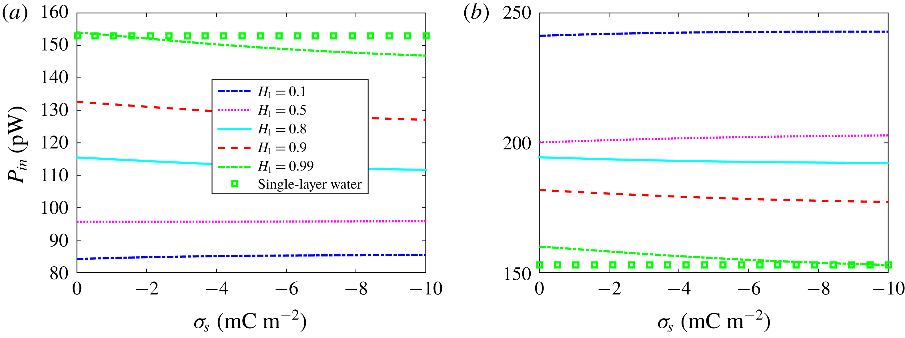
For unidirectional and steady two-layer Newtonian fluid flow between parallel plates with viscosities
 $\unicode[STIX]{x1D707}_{i}$
(
 $i=1,2$
), one has
 $$\begin{eqnarray}\displaystyle & \displaystyle P_{in}=\int _{V}u(y)\left(-\frac{\text{d}p}{\text{d}x}\right)\text{d}V=Q(-\unicode[STIX]{x0394}p), & \displaystyle\end{eqnarray}$$
 $$\begin{eqnarray}\displaystyle & \displaystyle P_{out}=\int _{V}\,j\left(\frac{\unicode[STIX]{x0394}\unicode[STIX]{x1D719}}{l}\right)\text{d}V=I(\unicode[STIX]{x0394}\unicode[STIX]{x1D719}), & \displaystyle\end{eqnarray}$$
 $$\begin{eqnarray}\displaystyle & \displaystyle P_{V}=\int _{0}^{l}\text{d}x\int _{0}^{w}\text{d}z\left[\int _{0}^{h_{1}}\unicode[STIX]{x1D707}_{1}\left(\frac{\text{d}u}{\text{d}y}\right)^{2}\text{d}x+\int _{-h_{2}}^{0}\unicode[STIX]{x1D707}_{2}\left(\frac{\text{d}u}{\text{d}y}\right)^{2}\text{d}x\right], & \displaystyle\end{eqnarray}$$
and
 $P_{E}=P_{in}-P_{out}-P_{V}$
. Under the maximum power generation condition, i.e.
 $\unicode[STIX]{x0394}\unicode[STIX]{x1D719}=-\unicode[STIX]{x0394}pL_{12}/2L_{22}$
, the input and output powers, and the viscous and electrical Joule heating dissipations can be expressed in terms of the phenomenological coefficients
 $L_{11}$
,
 $L_{12}$
and
 $L_{22}$
as
 $$\begin{eqnarray}\displaystyle & \displaystyle P_{in}=\frac{2-\unicode[STIX]{x1D6FC}}{2}L_{11}\unicode[STIX]{x0394}p^{2}, & \displaystyle\end{eqnarray}$$
 $$\begin{eqnarray}\displaystyle & \displaystyle P_{out}=\frac{\unicode[STIX]{x1D6FC}}{4}L_{11}\unicode[STIX]{x0394}p^{2}, & \displaystyle\end{eqnarray}$$
 $$\begin{eqnarray}\displaystyle & \displaystyle P_{E}=\frac{\unicode[STIX]{x1D6FC}L_{11}}{4L_{22}}L_{22}^{(2)}\unicode[STIX]{x0394}p^{2}, & \displaystyle\end{eqnarray}$$
 $$\begin{eqnarray}\displaystyle & \displaystyle P_{V}=\left[1-\unicode[STIX]{x1D6FC}+\frac{\unicode[STIX]{x1D6FC}L_{11}^{(1)}}{4L_{22}}\right]L_{11}\unicode[STIX]{x0394}p^{2}. & \displaystyle\end{eqnarray}$$
Here
 $\unicode[STIX]{x1D6FC}$
is the figure of merit, and
 $L_{11}$
,
 $L_{12}$
and
 $L_{22}$
are given in (3.12), (3.13) and (3.15), where
 $L_{22}$
is divided into two parts as
 $L_{22}=L_{22}^{(1)}+L_{22}^{(2)}$
according to the contributions from convection and electro-migration of ions, respectively, i.e.
 $$\begin{eqnarray}\displaystyle & \displaystyle L_{22}^{(1)}=\frac{w\unicode[STIX]{x1D700}_{1}^{2}}{lh\unicode[STIX]{x1D707}_{2}}\left(\frac{k_{B}T}{ze}\right)^{2}[\unicode[STIX]{x1D707}_{r}\,f_{1}+\unicode[STIX]{x1D700}_{r}\,f_{2}-\overline{A}_{1}^{2}(H_{2}+\unicode[STIX]{x1D707}_{r}H_{1})], & \displaystyle\end{eqnarray}$$
 $$\begin{eqnarray}\displaystyle & \displaystyle L_{22}^{(2)}=\frac{w\unicode[STIX]{x1D700}_{1}D_{-,1}}{2lh}K^{2}f_{3}+G_{w}. & \displaystyle\end{eqnarray}$$
Note that
 $P_{out}/P_{in}$
is exactly the efficiency of the system. In figure 11, we show the variations of the input power with the interface charge density
 $\unicode[STIX]{x1D70E}_{s}$
against different values of dimensionless thickness
 $H_{1}$
for the cases of
 $\unicode[STIX]{x1D707}_{r}>1$
and
 $\unicode[STIX]{x1D707}_{r}<1$
, respectively. It is observed that
 $P_{in}$
is almost a constant with respect to
 $\unicode[STIX]{x1D70E}_{s}$
, but depends strongly on
 $H_{1}$
. Furthermore, the effect of
 $H_{1}$
on the input powers is opposite for the viscosity ratios
 $\unicode[STIX]{x1D707}_{r}>1$
and
 $\unicode[STIX]{x1D707}_{r}<1$
, which can be attributed to the effect of
 $H_{1}$
on the velocity (see figures 4 and 7
a). In addition, the dependences of viscous dissipation and electrical Joule heating dissipation on the interfacial charges and interface location can be found in figures 6 and 9 in both cases.



