





Impact Statement
This work provides a detailed fluid-mechanical characterisation of laminar jet formation in square-edged orifice nozzles, a geometry widely used in laminar jet apparatus (LJA) mass transfer experiments but insufficiently understood. Using multiphase computational fluid dynamics simulations supported by targeted experiments, we resolve the near-nozzle flow, jet contraction, velocity profile development and jet breakup to assess the validity of long-standing assumptions employed in the design and interpretation of such experiments. Various flow conditions are analysed. The results clarify the mechanisms governing jet behaviour in a non-idealised LJA and provide a robust foundation for improving the modelling, operation and interpretation of mass transfer experiments therein.
1. Introduction
Accurate knowledge of gas–liquid mass transfer rates is essential for the design of many types of industrial equipment, including absorption and desorption columns and gas–liquid reactors. The efficiency of such processes is governed not only by fluid-dynamic conditions, but also by fundamental physico-chemical properties, such as diffusion coefficients and reaction rate constants in chemisorption. These fundamental properties are often determined in dedicated experiments, conducted in apparatuses where the fluid dynamics are well-characterised – a prerequisite for meaningful evaluation of the experimental data.
One of the most widely used devices for such studies is the laminar jet apparatus (LJA), introduced by Matsuyama (Reference Matsuyama1950). The LJA has been employed extensively to measure diffusion coefficients of gases in liquid mixtures (e.g. Onda et al. Reference Onda, Okamoto and Yamaji1960; Tang & Sandall Reference Tang and Sandall1985; Unver & Himmelblau Reference Unver and Himmelblau1964; Ying & Eimer Reference Ying and Eimer2012) as well as to investigate the enhancement of mass transfer by chemical reactions (e.g. Aboudheir et al. Reference Aboudheir, Tontiwachwuthikul, Chakma and Idem2003; Manogue & Pigford Reference Manogue and Pigford1960; Matsuyama Reference Matsuyama1950; Ramachandran et al. Reference Ramachandran, Aboudheir, Idem and Tontiwachwuthikul2006). Despite the long history of this apparatus, reliable and consistent mass transfer data remain surprisingly scarce (Bellaire et al. Reference Bellaire, Großmann, Münnemann and Hasse2022; Großmann et al. Reference Großmann, Bellaire, Hayer, Jirasek and Hasse2022; Hegely et al. Reference Hegely, Roesler, Alix, Rouzineau and Meyer2017; Putta et al. Reference Putta, Svendsen and Knuutila2017), underscoring the need not only for high-quality data but also for robust methods to obtain them.
In the LJA, a liquid jet is introduced into a gas-filled chamber through a nozzle. As it traverses the chamber, the liquid absorbs gas before exiting through a small funnel, which is designed to allow only the loaded liquid to leave while preventing gas entrainment. Gas–liquid mass transfer occurs across the surface of the jet. Since the chamber is typically filled with a pure gas, the main mass transfer resistance lies on the liquid side. The gas–liquid contact time can be controlled by adjusting the liquid flow rate and the jet length (i.e. the distance between the nozzle and the funnel). The chamber is usually operated at constant pressure (typically atmospheric), and the mass transfer rate is determined either by measuring the make-up gas required to replace the absorbed component or by analysing the composition of the liquid leaving the chamber. The entire system is thermostatted.
The LJA offers several distinctive advantages. One is the very short contact time between the gas and liquid phases – typically only a few milliseconds. This minimises gas uptake and thereby simplifies both the operation and the interpretation of experiments. In particular, this feature is advantageous in chemisorption studies, as the short contact times allow most reactions to be treated as (pseudo-)first-order reactions. Another important feature is the tractable mathematical description of the absorption process: the jet is typically assumed to be cylindrical with a uniform velocity profile, which allows the gas–liquid mass transfer to be modelled in a simple way in the reference frame of the moving liquid, without empirical parameters. This contrasts with other experimental set-ups, which often rely on simplified theories such as the two-film model and introduce uncertain parameters like the film thickness. In the present work, we examine the validity of these simplifying assumptions, which are critical to the interpretation of LJA experiments. Although the motivation for this work lies in gas–liquid mass transfer experiments, the present study is restricted to the hydrodynamics of the jet. The underlying assumption is that mass transfer does not significantly influence the fluid dynamics of the jet. This assumption is well justified for LJA experiments, where the concentrations of the diffusing components in the liquid phase are typically very low. A direct treatment of superimposed mass transfer is beyond the present scope and constitutes a natural extension for future work. The aim of this work is to establish a fluid-mechanical basis and a methodological blueprint for the rational design, operation and interpretation of LJAs.
The classical literature on free liquid jets is extensive: many authors have investigated the jet profile (e.g. Duda & Vrentas Reference Duda and Vrentas1967; Haustein et al. Reference Haustein, Harnik and Rohlfs2017; Scheuermann Reference Scheuermann1919; Weisbach, Reference Weisbach1855), jet instability and breakup (e.g. Birouk & Lekic Reference Birouk and Lekic2009; Grant & Middleman Reference Grant and Middleman1966; Rayleigh, Reference Rayleigh1878; Shibata et al. Reference Shibata, Koshizuka and Oka2004; Weber Reference Weber1931), nozzle flow (e.g. Dias & Vanden-Broeck Reference Dias and Vanden-Broeck1990; Lienhard & Lienhard Reference Lienhard and Lienhard1984; Ramamurthi & Nandakumar Reference Ramamurthi and Nandakumar1999) and velocity profiles (e.g. Lienhard Reference Lienhard1968; Richards & Scheele Reference Richards and Scheele1985) to name just a few, and in general, the effects of gravity, surface tension and viscosity on downstream jet development are well-understood (e.g. Clarke Reference Clarke1969; Joseph et al. Reference Joseph, Nguyen and Matta1983). However, the direct transfer of such results to LJAs remains non-trivial because most works do not address the full sequence of hydrodynamic processes relevant to a practical LJA operation and published models are often derived for idealised profiles or asymptotic parameter ranges. Hence, the present contribution does not revisit the problem in full generality, but rather examines how such phenomena manifest in the specific geometry and conditions relevant to LJA operation, with a focus on the entrance effects encountered in practice.
The nozzle geometry plays a central role for the LJA (Danckwerts Reference Danckwerts1970). We use the term ‘nozzle’ in a general sense here, to refer to the apparatus part from which the jet emanates. Various nozzle types have been used in the literature, including converging nozzles (e.g. bell-shaped, elliptical or other tapered profiles) (Clarke Reference Clarke1964; Cullen & Davidson Reference Cullen and Davidson1957; Diaz et al. Reference Diaz, Vega and Coca1988; Duda & Vrentas Reference Duda and Vrentas1968; Hofmeister & Kohlhaas Reference Hofmeister and Kohlhaas1965; Kramers et al. Reference Kramers, Blind and Snoeck1961; Onda et al. Reference Onda, Okamoto and Yamaji1960; Raimondi & Toor Reference Raimondi and Toor1959; Scriven & Pigford Reference Scriven and Pigford1958; Thomas & Adams Reference Thomas and Adams1965; Unver & Himmelblau Reference Unver and Himmelblau1964), sharp-edged nozzles (e.g. square-edged orifice plates) (Aboudheir et al. Reference Aboudheir, Tontiwachwuthikul, Chakma and Idem2004; Al-Ghawas et al. Reference Al-Ghawas, Hagewiesche, Ruiz-Ibanez and Sandall1989; Clarke Reference Clarke1964; Haimour & Sandall Reference Haimour and Sandall1984; Hershcovich et al. Reference Hershcovich, Merchuk and Tamir1982; Johnson & Davis Reference Johnson and Davis1996; Raimondi & Toor Reference Raimondi and Toor1959; Ruiz-Ibanez et al. Reference Ruiz-Ibanez, Bidarian, Davis and Sandall1991; Tang & Sandall Reference Tang and Sandall1985; Ying & Eimer Reference Ying and Eimer2012) and constant-diameter nozzles (e.g. capillary tubes or precision bores) (Brignole & Echarte Reference Brignole and Echarte1981; Raimondi & Toor Reference Raimondi and Toor1959). In some studies, the nozzle geometry is not specified at all. Raimondi & Toor (Reference Raimondi and Toor1959) compared multiple designs and reported the most reliable results with square-edged orifice plates, i.e. a thin plate with a circular hole that has neither bevelled nor rounded edges. The present work is focused exclusively on this nozzle type.
A central but often overlooked point is that the jet radius downstream of the nozzle is not known a priori and depends on the nozzle geometry as well as the flow within the nozzle. Here, we specifically address the question: Given a specific geometry, what jet radius is actually formed, and how does it evolve immediately downstream of the orifice?
Jet stability is also a key consideration in LJA operation. The well-known Rayleigh–Plateau instability (e.g. Chandrasekhar Reference Chandrasekhar2013) dictates that a cylindrical jet is unstable to axisymmetric disturbances with wavelengths greater than its circumference, which is basically always the case in LJAs. The surface waves increase in amplitude as capillary forces favour the reduced surface area of the jet. Inevitably, this instability will lead to fluid thread breakup. If the jet breaks up, the experiment must be stopped. Even prior to breakup, the growing perturbations can compromise results in several ways: they can prevent the clean capture of the jet in the funnel, and they can lead to a breakdown of the assumptions underpinning the theoretical evaluation. Thus, avoiding jet breakup is necessary but not sufficient; any significant instability must also be prevented. It is therefore essential to maintain the jet length well below the breakup length to ensure the integrity of the experimental conditions.
These considerations underline the importance of a detailed and physically accurate description of the jet hydrodynamics in LJAs. In particular, the validity of common assumptions – such as constant jet radius or uniform velocity profiles – has not been systematically assessed for the commonly used square-edged orifice nozzles. A deeper understanding of the jet formation, its stability and the associated flow field is therefore essential to ensure the reliability of LJA-based mass transfer experiments. The present study addresses this gap and provides a comprehensive basis for evaluating and improving LJA design and interpretation – both experimentally and through computational fluid dynamics (CFD). The full sequence of hydrodynamic processes is considered: the entire nozzle including the end of the feed line and the square-edged orifice, the complete jet up to the fluid thread breakup and the surrounding gas phase. The results provide guidance for apparatus design and interpretation, and a methodological basis for future optimisation studies.
2. Experiments
2.1. Set-up
Figure 1 gives an overview of the LJA used in this work. The liquid flow was driven by a piston mounted in a pneumatic cylinder, which was connected to a pressurised nitrogen gas cylinder. Special piston seals and guide rings minimised stick-slip effects and ensured a constant liquid flow rate, which was adjusted via a needle valve in the feed line. Both the cylinder and the feed line were thermostatted. The liquid flow rate and temperature were measured using a Coriolis mass flow meter (Bronkhorst, M54-RGD-22-O-S) with an uncertainty of
 $\pm$
0.2 % and a calibrated Pt100 resistance thermometer with an uncertainty of
 $\pm$
0.1 K.
Overview of the LJA. The liquid is coloured blue.

Figure 1 Long description
A diagram of a laminar jet apparatus. The liquid is colored blue. The apparatus includes a gas cylinder, piston cylinder, feed line, flow meter, jackscrew, thermometer for liquid, thermometer for gas, jet chamber, nozzle, camera, backlight, funnel, and discharge tank. The gas cylinder is connected to the piston cylinder, which feeds gas through the feed line and flow meter. The jackscrew is positioned above the jet chamber, which contains a nozzle. Thermometers for liquid and gas are placed near the jet chamber. A camera and backlight are positioned to observe the process. The liquid flows through the funnel into the discharge tank.
The feed line consisted of a stainless steel capillary tube (650 mm length, 5 mm inner diameter) that extended into the jet chamber, terminating in a nozzle from which the jet emerged. The jet chamber was made of glass and equipped with a double-walled jacket for thermostatisation. The temperature inside the chamber was monitored using a calibrated Pt100 resistance thermometer with an uncertainty of
 $\pm$
0.1 K. The vertical position of the nozzle was adjustable via a jackscrew, as the feed line was mounted in a movable assembly. This allowed the jet length (i.e. the distance between the nozzle and discharge funnel) to be varied from zero to approximately 100 mm. The vertical position of the nozzle was measured using a dial gauge (Käfer, MD 100 TB) with an uncertainty of
 $\pm$
0.03 mm. The nozzle consisted of a thin, square-edged orifice plate with a thickness of 0.1 mm and was mounted to the threaded tip of the capillary tube by a union nut. The orifice plate could be exchanged to vary the nozzle diameter
 $D_{0}$
; in this work, plates with
 $D_{0}=1.0$
mm and
 $D_{0}=1.9$
mm were used.
For the optical measurement of the jet shape, a monochrome CCD camera (AVT, Stringray F-046) equipped with a telecentric lens (Opto Engineering, RT-HR-4M-100) was mounted on a rail outside the chamber. A flat backlight illumination unit (CCS, TH-27X27RD) was mounted on the opposite side. This set-up allowed the jet to be imaged in a movable window along the vertical axis. The camera–lens combination provided a spatial resolution of 0.9358 µm pixel−1. A standard photograph of the backlit jet is shown exemplarily together with a high resolution image from the CCD camera in the supplementary material.
To determine the jet profile, multiple images were recorded between
 $y=0$
(at the orifice) and the breakup length of the jet, in 3 mm intervals. Each image was binarised using Otsu’s method (Otsu Reference Otsu1979), and an edge-detection algorithm (Danielsson & Seger Reference Danielsson and Seger1990) was applied to identify the pixels at the jet surface. The jet diameter at each axial position
 $y$
was calculated as the mean distance between the leftmost and rightmost surface pixels along the vertical resolution of each image. The resulting uncertainty in the determination of the jet diameter is approximately
 $\pm$
5 µm for steady conditions. At high jet lengths, the jet tends to become unstable due to the surface perturbations. In this regime, the jet contour observed by the CCD camera appears blurred and becomes difficult to evaluate. The numbers found for the (apparent) jet radius rapidly decrease under these conditions (see results). Furthermore, under the influence of the surface waves, it becomes increasingly difficult to manipulate the jet without splashing at the discharge funnel.
2.2. Overview
The experiments can be characterised by three dimensionless numbers, calculated at the nozzle: the Reynolds number Re, the Froude number Fr and the Weber number We:
 \begin{align} {\textit {Re}} = \frac {\rho \overline {u}_{0} D_{0}}{\eta } , \\[-10pt] \nonumber\end{align}
 \begin{align} {\textit {Fr}} = \frac {\overline {u}_{0}^{2}}{g D_{0}} , \\[-10pt] \nonumber\end{align}
 \begin{align} {\textit {We}} = \frac {\rho \overline {u}_{0}^{2} D_{0}}{\sigma } . \\[10pt] \nonumber\end{align}
Here,
 $\rho$
is the specific liquid density,
 $\eta$
the dynamic liquid viscosity,
 $\sigma$
the vapour–liquid surface tension,
 $\overline {u}_{0}$
the mean velocity at the nozzle exit,
 $D_{0}$
the nozzle diameter and
 $g=9.81\, \mathrm{m}\, \mathrm{s}^{-1}$
the gravitational acceleration. Only distilled water was used in the experiments; its thermophysical properties were taken from reference correlations (IAPWS 2014; Pátek et al. Reference Pátek, Hrubý, Klomfar, Součková and Harvey2009).
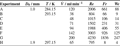
Table 1 summarises the investigated experimental conditions. A wide range of Reynolds, Froude and Weber numbers was covered in this work.
Overview of the experiments of the present work.

2.3. Computational fluid dynamics simulations
2.3.1. Set-up
Numerical simulations of the liquid jet were performed using the open-source CFD software OpenFOAM-v2212 (Weller et al. Reference Weller, Tabor, Jasak and Fureby1998) on a workstation equipped with an Intel Core i7-6700K processor (4.00 GHz) and 64 GB of RAM. The simulations were carried out for the same hydrodynamic conditions as the experiments, see table 1.
Both the liquid and the surrounding gas were treated as incompressible fluids with constant density. This assumption is valid even for the gas phase, as the pressure and temperature within the computational domain were basically constant. Although gas solubility is important for the actual application of the LJA, it was neglected in the simulations, as it has no significant effect on the jet hydrodynamics. The simulations were performed assuming isothermal conditions. The focus of this work is the steady-state flow in the absence of hydrodynamic instabilities.
The flow is treated as axisymmetric. Accordingly,
 $y$
denotes the axial coordinate in the direction of gravity and
 $r$
the radial coordinate measured from the symmetry axis. The simulation yields three field quantities: the fraction of the liquid in a given volume element (‘liquid volume fraction’)
 $\alpha$
, the pressure
 $p$
and the velocity vector
 $\boldsymbol{u}$
. The axial component of the velocity vector is denoted by
 $u_{y}$
. The governing equations are the continuity equation, the conservation of momentum and an equation describing the motion of the gas–liquid interface.
The continuity equation, i.e. the conservation of mass for incompressible flow, is
 \begin{equation} \boldsymbol{\nabla }\boldsymbol{\cdot }\boldsymbol{u} = 0 , \end{equation}
where
 $\boldsymbol{u}$
is the vector field of velocity. Assuming Newtonian behaviour with constant viscosity, the conservation of momentum is
 \begin{equation} \rho \left ( \frac {\partial \boldsymbol{u}}{\partial t} + \boldsymbol{u} \boldsymbol{\cdot } \boldsymbol{\nabla } \boldsymbol{u} \right ) = -\boldsymbol{\nabla } p + \mu \boldsymbol{\nabla }^{2} \boldsymbol{u} + \rho \boldsymbol{g} + \boldsymbol{f}_{\sigma } , \end{equation}
where
 $t$
is the time,
 $\rho$
is the density of the fluid,
 $p$
is the pressure,
 $\mu$
is the dynamic viscosity,
 $\boldsymbol{g}$
is the gravitational acceleration and
 $\boldsymbol{f}_{\sigma }$
is a term modelling the influence of the surface tension.
The interface is described by a volume-of-fluid (VOF) method, in which the scalar field
 $\alpha$
, describing the liquid volume fraction (1 = liquid, 0 = gas) in each cell, is subject to
 \begin{equation} \frac {\partial \alpha }{\partial t} + \boldsymbol{\nabla }\boldsymbol{\cdot }(\boldsymbol{u}\alpha ) = 0 . \end{equation}
The density
 $\rho$
in each cell was calculated from the liquid density
 $\rho _{1}$
and the gas density
 $\rho _{2}$
by
 \begin{equation} \rho = \alpha \rho _{1} + (1-\alpha )\rho _{2} . \end{equation}
For modelling the influence of the surface tension, which physically appears as a stress jump at the gas–liquid interface, the continuum surface force (CSF) method (Brackbill et al. Reference Brackbill, Kothe and Zemach1992) was used. In the CSF formulation, the interfacial stress balance is not imposed as an explicit sharp-interface boundary condition. Instead, the capillary force is distributed over the numerically smeared interface region and enters the momentum equation as a localised volumetric force (
 $\boldsymbol{f}_{\sigma }$
from (2.5)) proportional to the local curvature and directed normal to the interface
 \begin{equation} \boldsymbol{f}_{\sigma } = \sigma \kappa \boldsymbol{\nabla } \alpha , \end{equation}
where
 $\sigma$
is the surface tension of fluid 1 in contact with fluid 2 and
 $\kappa$
is the local surface curvature, calculated from
 \begin{equation} \kappa = - \boldsymbol{\nabla } \boldsymbol{\cdot } \boldsymbol{\hat {n}} = - \boldsymbol{\nabla } \boldsymbol{\cdot } \left ( \frac {\boldsymbol{\nabla } \alpha ^{*}}{\left | \boldsymbol{\nabla } \alpha ^{*} \right |} \right ) , \end{equation}
where
 $\boldsymbol{\hat {n}}$
is the unit vector normal to the interface and
 $\alpha ^{*}$
is a smoothed volume fraction. Only in cells at the interface is
 $\boldsymbol{\nabla } \alpha$
non-zero; thus, the capillary force contributes to the momentum equation only in this interfacial region.
The simulations were carried out in dimensional form, but for interpretation, the governing equations may be cast in non-dimensional form using the characteristic scales
 $\overline {u}_{0}$
and
 $D_{0}$
and the liquid density
 $\rho _{1}$
as a reference, yielding the Reynolds, Froude and Weber numbers defined in (2.1)–(2.3) (cf. supplementary material).
The numerical schemes used in combination with the model equations above (e.g. for interpolation, surface normal gradients and discretisation) are specified in the supplementary material. The simulations were carried out with OpenFOAM’s interIsoFoam solver, which is a combination of the interFoam solver with the isoAdvector interface advection method (Reference Roenby, Bredmose, Jasak, Miguel Nóbrega and Jasak2019, Roenby et al. Reference Roenby, Bredmose and Jasak2016). The numerical methods have been validated and benchmarked extensively in the literature (e.g. Gamet et al. Reference Gamet, Scala, Roenby, Scheufler and Pierson2020; Lippert et al. Reference Lippert, Tolle, Dörr and Maric2022; Marić et al. Reference Marić, Kothe and Bothe2020; Roenby Reference Roenby2018; Yahyaee et al. Reference Yahyaee, Bahman and Sørensen2022). The isoAdvector method is preferred to MULES (Multidimensional Universal Limiter for Explicit Solution) – which is the default interface capturing method for the interFoam solver – as MULES can lead to so-called spurious currents (i.e. non-physical artefacts at the interface), and interIsoFoam often bests interFoam in speed and convergence (Gamet et al. Reference Gamet, Scala, Roenby, Scheufler and Pierson2020; Roenby et al. Reference Roenby, Larsen and Bredmose2017; Yahyaee et al. Reference Yahyaee, Bahman and Sørensen2022). These findings were confirmed in preliminary studies that showed that the interIsoFoam solver gave better results, especially in the region of the jet surface.
The numerical settings (mesh resolution, time stepping and solver tolerances) were chosen conservatively with a focus on robustness and accuracy rather than computational efficiency. Convergence was assessed by monitoring the iteration history and residuals of all governing equations, which showed stable and well-converged behaviour. In addition, selected parameters were varied in preliminary studies to confirm that the chosen settings are appropriate.
The time steps were automatically adjusted (with an upper limit
 $\Delta _{\mathrm{max}}t = 10$
µs) according to the maximum Courant number of
 ${\textit {Co}}_{\mathrm{max}} = 0.5$
. This bounded adaptive time-stepping strategy together with strict solver tolerances (see supplementary material) was used to ensure numerical stability of the transient simulation and a controlled temporal resolution of the gas–liquid interface. The calculated time steps were saved to memory in write intervals of
 $\Delta _{\text{w}}t \approx \overline {u}_{0} / \left (100\max (y)\right )$
, where
 $\overline {u}_{0}$
is the average axial velocity at the nozzle and
 $\max (y)$
is the length up to which the jet is simulated, i.e. 50 mm for scenarios B, C and H (cf. table 1) and 100 mm otherwise. The simulations were stopped after approximately twice the time a volume element in the centre of the jet needs to traverse the simulation volume in vertical direction. The comparison with the experimentally measured jet profiles provides a practical validation strategy of the present numerical set-up.
2.3.2. Simulation domain and mesh
Due to the laminar jet chamber’s large size in comparison with the jet itself, the simulation domain is limited only to the area of interest, which includes the nozzle region, the liquid jet and the gas–liquid interface, as well as the nearby gas phase. The simulation domain is cut off (in the capillary and in the gas phase) at a point where the influences from the nozzle and jet have well subsided (cf. results in sections 3.2–3.3). The schematic in figure 2 shows the simulation domain in relation to the entire jet chamber.
Schematic of a laminar jet chamber (not to scale) that shows the circulating gas flow induced by the liquid jet. The simulation domain is shown in red.

The coordinate origin is defined as the point on the symmetry axis just below the nozzle, where the free-falling jet begins. In OpenFOAM, the equations are implemented on the underlying Cartesian mesh, but in the present manuscript, we denote the radial coordinate by
 $r$
for physical clarity and consistency with the axisymmetric jet geometry.
A hexahedral, wedge-shaped mesh with wedge angle of 4
 $^\circ$
was constructed using the blockMesh utility. The full mesh consists of 153 540 cells. The standard elongation of the bounding rectangle was 10 mm in the
 $r$
-direction and 105 mm in the
 $y$
-direction. The mesh is graded to provide a higher resolution in areas of high interest. This includes grading in the
 $r$
-direction for blocks where the jet surface is expected and for blocks near the boundaries of the simulation domain, and grading in the
 $y$
-direction for blocks surrounding the nozzle. Details, including a visual representation of the blocks comprising the mesh, are provided in the supplementary material.
2.3.3. Initial and boundary conditions
A boundary condition must be specified for each of the fields (
 $\alpha$
,
 $p$
and
 $\boldsymbol{u}$
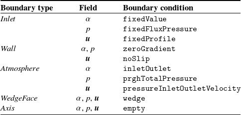
) on every face of the mesh. There are five different types of boundaries in the present problem, which are labelled here as: inlet, wall, atmosphere, wedgeFace and axis. The respective boundary conditions (in OpenFOAM nomenclature) that are applied on these boundary types are given in table 2. For more information, see the supplementary material. The mesh faces are assigned to the boundary types from table 2. A visual depiction of the mesh faces and respective boundary types is provided in the supplementary material (see figure S.2). The inlet is modelled with a constant Hagen–Poiseuille inflow profile of the liquid (
 $\alpha = 1$
). The wall of the capillary as well as the nozzle’s orifice plate are modelled with no-slip conditions. Finally, the atmosphere boundary type is used for the faces where the simulation domain clips the gas phase of the chamber and where the liquid jet discharges into the collector. Here, the Dirichlet boundary conditions for
 $\alpha$
and
 $p_{\mathrm{rgh}}$
take the values 0 and 101 325 Pa, respectively. To model the rotational symmetry of the problem, the collapsed faces at the axis of symmetry are assigned the empty boundary type and all faces in the paper plane (see figure S.2 of the supplementary material) are assigned the wedgeFace boundary type.
Boundary types and boundary conditions of all block faces in the simulation. Physical explanations of the boundary conditions are given in the supplementary material.

The initial
 $\alpha$
field is set such that it is 1 (liquid) everywhere in the capillary tube, i.e. for
 $y \leq -0.1$
, and 0 (gas) everywhere else at the start of the simulation. The initial
 $p_{\mathrm{rgh}}$
and
 $\boldsymbol{u}$
fields are 101 325 Pa and 0, respectively, throughout the entire domain.
The temperature is no variable in the simulation. It only comes into play through the fluid properties, which are temperature-dependent.
2.3.4. Post-processing
Post-processing of the CFD simulations was carried out with the software ParaView. The jet profile was determined by the
 $\alpha = 0.5$
isoline.
The uniformity of the axial velocity profile in the jet is described by the flow uniformity index
 $\gamma$
, defined for a constant height
 $y$
as (Munnannur et al. Reference Munnannur, Cremeens and Liu2011)
 \begin{equation} \gamma = 1 - \frac {1}{2 \overline {u}_{\mathrm{y}}} \frac {\sqrt {\sum w_{i} (u_{\mathrm{y},i}-\overline {u}_{\mathrm{y}})^2}}{\sum w_{i}} , \end{equation}
where
 $u_{\mathrm{y},i}$
is the axial velocity in a cell,
 $\overline {u}_{\mathrm{y}}$
is the weighted average of all
 $u_{i}$
and
 $w_{i}$
is the weight of each individual cell. Here, the cells were weighted by
 $\alpha$
(as to disregard the gas phase) and the cell area, i.e.
 $w_{i} = \alpha _{i}A_{i}$
, where
 $A_{i}$
is the cell area perpendicular to the
 $y$
-axis.
The upper limit of the flow uniformity index is
 $\gamma = 1$
, which corresponds to a perfectly uniform flow profile. For a perfect parabolic flow profile, the value is
 $\gamma = 1-\sqrt {1/12} \approx 0.71$
. The flow uniformity index may become negative for velocity distributions with extremely high variances, e.g. for reversed flow conditions (Munnannur et al. Reference Munnannur, Cremeens and Liu2011).
Only time steps for which the leading edge of the jet left the simulation domain (at its lower end) were considered in the post-processing. We report the time-averaged values for all results, with the standard deviation as a measure of uncertainty, so that the results represent the developed quasi-stationary regime. The only exception to this is the breakup length
 $y_{\mathrm{BU}}$
, which was determined as the smallest
 $y$
-coordinate where the jet becomes discontinuous (i.e. where the jet radius first becomes zero) over all time steps.
3. Results and discussion
3.1. Overview
In the present work, both simulated and experimental data were obtained to analyse the hydrodynamics of the laminar jet. Mass transfer was not addressed directly. Experimental data are available only for the jet profiles (given here as the jet radius as a function of axial distance from the nozzle), while the simulations provide also the pressure and velocity fields for both the liquid jet and the surrounding gas phase. For each experiment from table 1, a corresponding simulation was carried out. The discussion focuses primarily on the velocity profiles within the jet and the jet profile; results concerning the gas phase are reported only briefly.
The experimental and simulated data for the jet profiles are provided in numerical form in the supplementary material. In addition, the OpenFOAM input files used to generate the field data are also included.
For the discussion of the results, we follow the flow and begin with the nozzle region, including the initial contraction of the jet at the nozzle exit. This is followed by an analysis of the jet profile. The contraction increases downstream due to the combined effects of surface tension, gravity and internal momentum transfer. The latter also causes the initially non-uniform velocity profile to evolve toward plug flow. At a finite axial distance, jet instabilities grow to the point of fluid thread breakup. Finally, the implications of these findings for the design and interpretation of LJA experiments are discussed.
Where possible, the findings are compared with results from the literature. However, only correlations applicable to the hydrodynamic conditions investigated in the present work were considered.
Figure 2 illustrates the liquid and gas phase flows within a laminar jet chamber and the simulation domain.
3.2. Gas phase
The flow in the gas phase is induced by the motion of the liquid jet. In the immediate proximity of the gas–liquid interface, the gas phase is accelerated to nearly the same axial velocity as the jet surface. While the gas moves downward in the chamber near the jet, it moves upward near the chamber’s jacket, forming closed streamlines (outside of the simulated domain, cf. figure 2).
Figure 3 shows a result for the velocity field in the liquid and the gas phase obtained by the CFD simulation. The data are from a snapshot of simulation scenario C and is representative of the typical behaviour during LJA operation. A video of the simulation is provided in the supplementary material.
Simulation of the central part of the laminar jet chamber, the dark grey area is not part of the simulation domain. The visualisation is mirrored at the
 $y$
-axis: the right half is coloured by the flow velocity in the gas and liquid phase, the left half shows the morphology of the liquid jet using the liquid volume fraction
 $\alpha$
(blue: liquid, white: gas). The jet is outlined by the black
 $\alpha = 0.5$
isoline. Data from a snapshot of simulation scenario C after 0.0882 s. Only the upper part, where the jet is stable, is interesting for LJAs. A small red rectangle marks the nozzle area that is investigated in more detail in figure 4.

The simulation domain covers only the central part of the chamber, near the laminar jet. The gas enters the simulation domain through the top mesh faces and leaves through the bottom mesh faces (both are assigned an atmosphere-type boundary condition, see figure S.2 of the supplementary material). Radial flow is negligible. The boundary layer, in which the gas is accelerated to almost the velocity of the jet, grows with the axial distance from the nozzle. Near the nozzle, where the boundary condition is wall, the gas remains largely quiescent, as expected. At the point of fluid thread breakup (approximately in the middle of figure 3) and beyond, the significant production of swirl in the gas phase can be seen by the strong gradients in the velocity field.
Only the results for the upper part of the jet, before the fluid thread breakup, are of interest for mass transfer experiments. Hence, the simulation results beyond the breakup length are not discussed in the subsequent sections.
3.3. Laminar jet in the nozzle region
The simulation results in the immediate vicinity of the nozzle are of particular interest, as this region is difficult to access experimentally and strongly influences the downstream jet behaviour. Simulation results from this region from a typical experiment (scenario D, cf. table 1) are shown in figure 4, presenting the velocity field and flow streamlines. The abrupt reduction in cross-sectional area leads to a sharp redirection and a significant acceleration of the flow. Furthermore, flow separation is observed (the vena contracta effect) at the inner edge of the nozzle orifice, resulting in the formation of a localised recirculation zone. To illustrate this feature, a streamline close to the inner edge of the orifice is highlighted in figure 4. The flow separation is closely related to the flow contraction of the liquid jet at the nozzle exit. The flow separation also influences the velocity profile at the nozzle exit, leading to slow flow near the vapour–liquid interface, see figure 4. Due to viscous momentum transfer, the velocity in the free jet becomes more uniform as the distance from the nozzle exit grows. This is discussed in more detail in section 3.6.
Simulation results for the flow velocity magnitude (colour coded) and streamlines in the nozzle region of the laminar jet. The orifice plate is shown as a grey bar. Flow separation is induced by the inner edge of the orifice plate, resulting in a localised recirculation zone. The white area is the gas phase; the position of the gas–liquid interface was calculated here from
 $\alpha = 0.5$
. As a reference, a streamline close to the inner edge of the orifice is highlighted in orange. The simulation results correspond to experiment D from table 1.

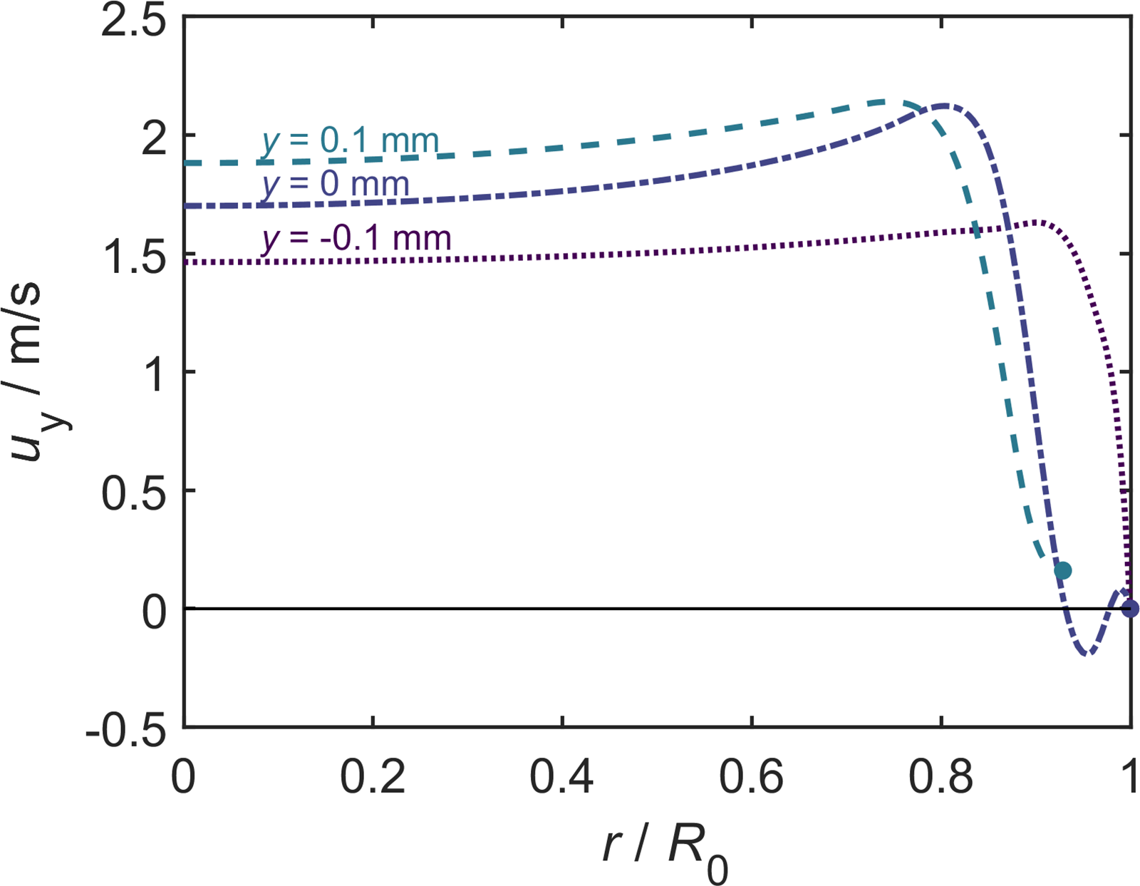
For an in depth discussion, figure 5 shows axial velocity profiles in the nozzle orifice and the jet taken from the same simulation scenario as in figure 4. The profiles
 $u(r)$
are shown for three locations: the upper and the lower edge of the nozzle orifice (
 $y=-0.1$
mm and
 $y=0$
, respectively) as well as one nozzle length downstream (
 $y=0.1$
mm). All profiles are uniform for small values of the radius
 $r$
but differences are observed as
 $r$
approaches the radius of the orifice
 $R_{0}$
. At the upper edge of the orifice (
 $y=-0.1$
mm), the axial velocity simply declines near the wall where the no-slip condition applies. At the lower edge (
 $y=0$
), backflow is observed near the wall. Down the jet, at
 $y=0.1$
mm (where jet contraction is observed), the velocity profile is still strongly non-uniform with decreasing velocity near the vapour–liquid interface.
Simulated axial velocity profiles in the nozzle and the liquid jet near the nozzle for simulation scenario D. The profiles are shown for three locations: at the upper and the lower edge of the orifice plate (
 $y=-0.1$
mm and
 $y=0$
, respectively) as well as one nozzle length downstream (
 $y=0.1$
mm). Here,
 $R_{0}$
is the nozzle radius.

Zoom into the simulated area of flow separation around the orifice plate (grey) with results from individual simulation scenarios as coloured lines. Left: streamlines passing just by the top inner edge of the orifice plate. Right: jet surface.

Figure 6 gives an overview of the results of the simulation of the nozzle region with a focus on the flow separation and the resulting recirculation zone. The lines in figure 6 correspond to the scenarios A–G (cf. table 1). The extent of the recirculation zone is indicated by its boundaries: in the left plot, the reference streamline passing near the inner edge of the nozzle orifice is shown, and in the right plot, the position of the gas–liquid interface (
 $\alpha = 0.5$
contour) is shown for each scenario. In most scenarios, the entire bore of the orifice is wetted, and the three-phase line (where gas, liquid and solid are in contact) coincides with the outer edge of the nozzle orifice. Only for very high Reynolds numbers (scenarios F and G), the three-phase line retracts into the bore. Here, the contact angle between the interface and the wall is imposed via the zeroGradient boundary condition for
 $\alpha$
and equates to 90
 $^\circ$
. The retraction of the three-phase line leads to a reduced size of the recirculation zone. The spatial extent of this area is visualised for each scenario (including scenario H, in which the nozzle geometry differed) individually in the supplementary material. The exact three-phase line position is sensitive to the wall wetting model and to dynamic contact-line effects, which are represented only in simplified form in the present VOF simulations, and a more refined treatment may improve the local prediction of interface attachment at the orifice. However, the main hydrodynamic findings, namely flow separation and strong initial jet contraction, are robust. The main message from the present study is that, while for the studied conditions, the three-phase line is usually located at the nozzle exit, it may retract into the bore at high flow velocities.
3.4. Jet profile
Figure 7 presents the simulated jet profiles for scenarios A–H, along with the corresponding experimental results from this work and results from the model of Duda & Vrentas (Reference Duda and Vrentas1967, Reference Duda and Vrentas1968). Normalised coordinates are used: the jet radius
 $R$
is normalised with the orifice diameter
 $R_{0}$
and the axial distance from the nozzle
 $y$
is normalised with the breakup length
 $y_{\mathrm{BU}}$
determined in the CFD simulations, which is reported for each experiment in figure 7. For more information on the breakup, see section 3.5. The increasing standard deviation of the simulation results (cf. section 2.3.4) for large values of
 $y/y_{\mathrm{BU}}$
are caused by the surface waves of the jet that are precursors of the fluid thread breakup.
Results for the jet profile in all studied cases (A–H, see table 2): (
 $\bigcirc$
) experimental data (connected by a black line as a guide for the eye), (
 ) CFD simulation, (
 ) model of Duda & Vrentas (Reference Duda and Vrentas1967, Reference Duda and Vrentas1968), (
 ) modified model of Duda & Vrentas (Reference Duda and Vrentas1967, Reference Duda and Vrentas1968) (this work). The grey shaded area is the standard deviation of the CFD simulations over multiple time steps.

Figure 7 Long description
Eight panels of line graphs depict the jet profile in various studied cases. Each panel shows the comparison between experimental data, CFD simulations, and models. The x-axis represents the normalized radial position (r/R0), and the y-axis represents the normalized axial position (y/yBU). Panel A shows a jet profile with yBU = 79.4 mm, Panel B with yBU = 28.5 mm, Panel C with yBU = 33.1 mm, Panel D with yBU = 49.6 mm, Panel E with yBU = 67.3 mm, Panel F with yBU = 82.3 mm, Panel G with yBU > 100 mm, and Panel H with yBU = 18.7 mm. The experimental data are represented by blue circles connected by a black line as a guide for the eye. The CFD simulation results are shown as a solid blue line, the model of Duda & Vrentas (1967, 1968) as a dashed black line, and the modified model of Duda & Vrentas (1967, 1968) as a red dashed line. The grey shaded area indicates the standard deviation of the CFD simulations over multiple time steps.
For the standard nozzle (scenarios A–G), the vena contracta effect leads to an important deviation of the radius of the jet leaving the nozzle from the radius of the orifice: the initial jet radius is only approximately 80 %–85 % of the orifice radius. With increasing distance from the nozzle, the jet radius decreases further, due to the combined action of velocity relaxation, gravity and surface tension, but this decrease is less important than that due to the vena contracta effect. The results for simulation scenario H differ strongly from the rest, which is a result of the different nozzle geometry. The agreement between measured and simulated jet profiles provides the principal validation of the present CFD set-up.
Various methods have been proposed in the literature to predict the jet profile. The simplest approach assumes a uniform velocity profile at the nozzle and neglects both gravity and surface tension, leading to a cylindrical jet of constant radius equal to the nozzle radius (Danckwerts Reference Danckwerts1970). This is obviously an oversimplification and might thus introduce inaccuracies in the evaluation of LJA experiments.
Several more advanced models accounting for gravity and surface tension have been proposed (e.g. (Kurabayasi Reference Kurabayasi1959; Lienhard Reference Lienhard1968; Massalha & Digilov Reference Massalha and Digilov2013; Scheuermann Reference Scheuermann1919; Weisbach, Reference Weisbach1855)). Massalha & Digilov (Reference Massalha and Digilov2013) showed that the models proposed by many authors can be cast into a common dimensionless form with a gravity term and a capillary correction, which has an asymptotic behaviour of
 $R' \sim (y'/{\textit {Fr}})^{-1/4}$
, where the superscript
 $'$
indicates the dimensionless jet radius and length. The same asymptotical behaviour was rigorously derived and experimentally verified by Joseph et al. (Reference Joseph, Nguyen and Matta1983) for jets of liquid into air. A more general treatment of the jet profile was given by Duda & Vrentas (Reference Duda and Vrentas1967, Reference Duda and Vrentas1968), who introduced a model applicable to arbitrary entry profiles (see supplementary material for the equations). In the present work, that model was used under the assumption of a uniform entry profile. Since our detailed comparison is carried out with the model of Duda & Vrentas (Reference Duda and Vrentas1967, Reference Duda and Vrentas1968), which reproduces the downstream asymptotic regime mentioned above, the related theories are not discussed separately here.
Figure 7 shows the predictions of the model of Duda & Vrentas (Reference Duda and Vrentas1967, Reference Duda and Vrentas1968) for all eight scenarios. The comparison with the experimental data and the CFD simulation results reveals that the model strongly overpredicts the jet radius. While the trend is predicted fairly well, the results are shifted to radii that are too high. The main reason for this is that the model does not account for the initial contraction at the nozzle due to the vena contracta effect. We therefore propose a simple modification of the model: instead of using the geometric nozzle radius
 $R_{0}$
, we propose to use an effective initial jet radius
 $R_{0}^{*}$
that accounts for the initial contraction. The question is here, how to predict the ratio
 $R_{0}^{*} / R_{0}$
. The results will depend on the nozzle type and dimensionless numbers characterising the flow. We demonstrate the feasibility of finding suitable correlations for the standard nozzle we have used here in the experiments A–G. For these experiments, we have determined the value of
 $R_{0}^{*}$
from an extrapolation of the experimental data for
 $R(y)$
to
 $y=0$
. We have then plotted the results for
 $R_{0}^{*}$
as a function of Re and found a reasonable correlation. Details are given in the supplementary material. The effective nozzle radius obtained from that correlation was then used as input for the model of Duda & Vrentas (Reference Duda and Vrentas1967, Reference Duda and Vrentas1968) to predict the jet profile. The initial velocity was also adjusted accordingly:
 $\overline {u}_{0}^{*} = \dot {V} / (\pi ( R_{0}^{*} )^{2} )$
. The results are shown in figure 7 and agree well with the experimental data; the mean absolute error is always below 3 %.
3.5. Jet instability and breakup
As the distance from the nozzle increases, the jet tends to become instable: surface waves increase in amplitude until the point of fluid thread breakup. Jet instability must be avoided in mass transfer experiments with the LJA.
Owing to its relevance in many industrial applications, the breakup of liquid jets has been extensively studied in the literature (e.g. Cramer et al. Reference Cramer, Berüter, Fischer and Windhab2002; Debler & Yu Reference Debler and Yu1988; Eggers Reference Eggers1997; Eroglu et al. Reference Eroglu, Chigier and Farago1991; Grant & Middleman Reference Grant and Middleman1966; Kalaaji et al. Reference Kalaaji, Lopez, Attané and Soucemarianadin2003; Kang et al. Reference Kang, Yu, Liu and Tao2023; Leroux et al. Reference Leroux, Dumouchel and Ledoux1997; Lienhard & Day Reference Lienhard and Day1970; Lin & Reitz Reference Lin and Reitz1998; Ohnesorge Reference Ohnesorge1936; Sallam et al. Reference Sallam, Dai and Faeth2002; Umemura Reference Umemura2011; Weber Reference Weber1931; Zhan et al. Reference Zhan, Kuwata, Maruyama, Okawa, Enoki, Aoyagi and Takata2020). While several empirical correlations for
 $y_{\mathrm{BU}}$
have been proposed – typically tailored to specific experimental configurations – there is still no general consensus on the influence of the various factors leading to jet breakup, let alone a universally applicable correlation to predict it (Birouk & Lekic Reference Birouk and Lekic2009).
The experiments of the present work give only qualitative information on the jet instability, as the temporal resolution of the images of the camera was not sufficient to resolve the highly dynamic surface waves. These fast changes in the jet contour lead to measurement artefacts in the form of blurred images approaching the breakup length. Details are given in the supplementary material. The CFD simulations also show these surface waves, which manifest in the data as a strongly increasing standard deviation of the jet radius, as shown in figure 7. In contrast to the experiments, the breakup length can be determined directly from CFD; it is the lowest
 $y$
coordinate at which the actual jet radius
 $R$
first becomes zero (i.e. the surface waves reach an amplitude equivalent to the mean jet radius) for any time step in the simulation.
The experimental information regarding jet breakup can be summarised as follows: for scenarios B and C, the experimental results confirm the CFD prediction, for scenarios D, E and H, the experiments indicate a slightly higher breakup length. For the remaining experiments, the jet was shorter than the simulated breakup length and there was no indication of a breakup in the experiments.
The observed instability mechanism is consistent with a Rayleigh–Plateau-type capillary instability. Classical theory predicts, for an inviscid cylindrical jet, a fastest-growing disturbance wavelength of approximately
 $9R$
(Chandrasekhar Reference Chandrasekhar2013). Our CFD results show the characteristic bulge-neck-type structures and their axial spacing are of the same order of magnitude as the predicted wavelengths, as can be seen qualitatively in figure 3. The observed growth of the surface waves with jet length (cf. figure 7) is also consistent with the expected capillary instability and culminates in a pinch-off of the liquid thread. Deviations from idealised Rayleigh–Plateau theory are expected, because the present jet is accelerating, viscous and of non-uniform velocity. Accordingly, we employ it here as an explanatory framework rather than a predictive model; instead, we quantitatively compare our results with existing correlations for the breakup length at a macroscopic, phenomenological level.
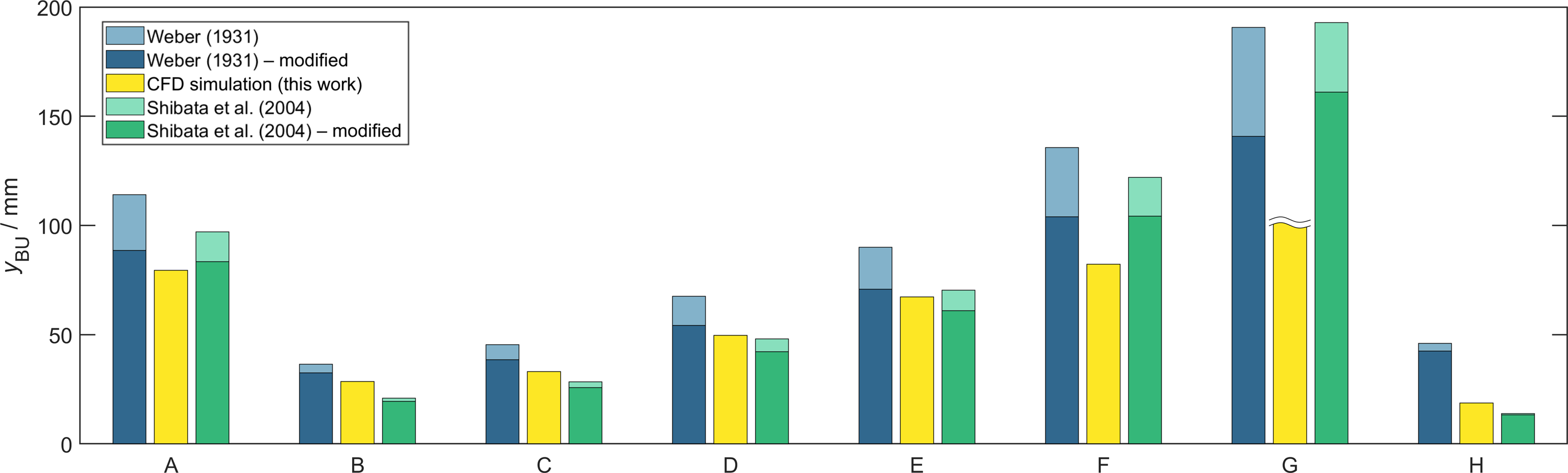
Figure 8 compares the CFD simulation results for the breakup length in all studied scenarios with predictions obtained with the models of Shibata et al. (Reference Shibata, Koshizuka and Oka2004) and Weber (Reference Weber1931), which were chosen as they are simple correlations, easy to apply and are representative of early and more recent work. The models have the forms
 $y_{\mathrm{BU}}/R_{0} = f({\textit {Re}}, {\textit {We}})$
and
 $y_{\mathrm{BU}}/R_{0} = f({\textit {Fr}}, {\textit {We}})$
, respectively. Other similar correlations were considered in preliminary work and showed no improvements. More complex models of the jet breakup were not considered here for the sake of simplicity.
Comparison of the breakup lengths determined in the CFD simulations of scenarios A–H (see table 1) with results from correlations of Shibata et al. (Reference Shibata, Koshizuka and Oka2004) and Weber (Reference Weber1931). The light-shaded bars are results from the original correlations, the dark-shaded bars are calculated with a scaled jet diameter accounting for the vena contracta effect. In scenario G, no jet breakup was observed within the simulation domain, which was 100 mm from the nozzle.

Each of the models was used in two versions: one is the original version, in which the initial jet radius is simply set equal to the radius of the nozzle bore
 $R_{0}$
, the other is a modification, in which the vena contracta effect is considered and the nozzle bore
 $R_{0}$
and velocity
 $\overline {u}_{0}$
were replaced by the effective initial jet radius
 $R_{0}^{*}$
and effective velocity
 $\overline {u}_{0}^{*}$
from section 3.4 (see also the supplementary material). The correlation itself remained unchanged in both cases.
For the purposes of the following discussion, we will treat the CFD simulation results for the breakup length as the ground truth. The original model of Weber (Reference Weber1931) always overestimates the breakup length, more so with increasing Re. An exception is scenario H, which is significantly overestimated despite low Re and We values. Accounting for the vena contracta effect strongly improves the predictions, which were found to be remarkably precise in most of the adjusted cases. The predictions obtained with the original version of the more recent model of Shibata et al. (Reference Shibata, Koshizuka and Oka2004) sometimes underestimate and sometimes overestimate the CFD results; for low values of Fr,
 $y_{\mathrm{BU}}$
is underestimated and for high values of Fr, it is overestimated. The agreement is slightly better than for the original version of Weber’s (Reference Weber1931) model. Accounting for the vena contracta effect always leads to smaller breakup lengths and is only beneficial in the scenarios with high Fr.
For practical LJA operation, the relevant issue is not just the ultimate breakup length, but also the rapid amplitude increase of surface waves near the breakup length, large enough to interfere with reliable jet capture at the funnel, promote splashing, and compromise the assumptions underlying the evaluation of the experiments. Since even an ideal, i.e. perfectly cylindrical, thin liquid jet is ultimately unstable to axisymmetric disturbances, breakup cannot be eliminated in principle, but its practical consequences can be mitigated by operating well below the breakup length. The results in figure 8 therefore provide guidance for selecting hydrodynamic conditions, like high-Re laminar flow, to increase the usable jet length and minimise the severity of pre-breakup disturbances under experimentally relevant conditions.
Simulated radial profile of axial velocity at three selected positions (a, b, c) in simulation scenario D (left). The positions correspond to
 $y=0.1$
mm,
 $y=5.5$
mm and
 $y=38$
mm, respectively. The simulated flow uniformity index as a function of axial distance is shown on the right; the grey shaded area is the standard deviation over all time steps.

3.6. Velocity profiles
In the following, we analyse how the velocity profile in the jet evolves under different hydrodynamic conditions, based on the CFD simulations. Along the jet axis, the flow undergoes an asymptotic transition from the initial velocity profile (see section 3.3) to a plug flow, eventually interrupted by the jet breakup. To quantify the relaxation toward plug flow, we use the flow uniformity index
 $\gamma$
defined in (2.10).
The left plot of figure 9 shows the radial profiles of the axial velocity
 $u_{\mathrm{y}}$
at three selected positions (a, b, c) for simulation scenario D. The evolution of the flow uniformity index as a function of the axial position is shown in the right plot of figure 9. Position (a) is located
 $0.1$
mm below the nozzle and has a strongly non-uniform velocity profile that still resembles that inside the nozzle, see figure 6. Further downstream, the profiles relax towards a uniform plug profile (corresponding to a flow uniformity index
 $\gamma = 1$
), but slight deviations from plug flow are still present even shortly before the jet breakup.
Simulated flow uniformity index as a function of the axial distance from the nozzle normalised by the breakup length for simulation scenarios A–H. For scenario G, in which no jet breakup was observed, the full jet length in the simulation domain was used for the normalisation. The grey shaded area is the standard deviation. Its increase is reflective of the surface waves in the jet.

Figure 10 Long description
Eight line graphs depict the simulated flow uniformity index as a function of the axial distance from the nozzle normalized by the breakup length for different simulation scenarios. Panel A: The line graph shows the flow uniformity index for scenario A. The x-axis is labeled y/y_BU and ranges from 0 to 1. The y-axis is labeled with a symbol that appears to represent the flow uniformity index and ranges from 0.8 to 1. The graph shows a relatively stable flow uniformity index with minor fluctuations. Panel B: The line graph shows the flow uniformity index for scenario B. The x-axis is labeled y/y_BU and ranges from 0 to 1. The y-axis is labeled with the same symbol and ranges from 0.8 to 1. The graph shows a stable flow uniformity index with minor fluctuations. Panel C: The line graph shows the flow uniformity index for scenario C. The x-axis is labeled y/y_BU and ranges from 0 to 1. The y-axis is labeled with the same symbol and ranges from 0.8 to 1. The graph shows a stable flow uniformity index with minor fluctuations. Panel D: The line graph shows the flow uniformity index for scenario D. The x-axis is labeled y/y_BU and ranges from 0 to 1. The y-axis is labeled with the same symbol and ranges from 0.8 to 1. The graph shows a stable flow uniformity index with minor fluctuations. Panel E: The line graph shows the flow uniformity index for scenario E. The x-axis is labeled y/y_BU and ranges from 0 to 1. The y-axis is labeled with the same symbol and ranges from 0.8 to 1. The graph shows a stable flow uniformity index with minor fluctuations. Panel F: The line graph shows the flow uniformity index for scenario F. The x-axis is labeled y/y_BU and ranges from 0 to 1. The y-axis is labeled with the same symbol and ranges from 0.8 to 1. The graph shows a stable flow uniformity index with minor fluctuations. Panel G: The line graph shows the flow uniformity index for scenario G. The x-axis is labeled y/y_BU and ranges from 0 to 1. The y-axis is labeled with the same symbol and ranges from 0.8 to 1. The graph shows a stable flow uniformity index with minor fluctuations. Panel H: The line graph shows the flow uniformity index for scenario H. The x-axis is labeled y/y_BU and ranges from 0 to 1. The y-axis is labeled with the same symbol and ranges from 0.8 to 1. The graph shows a stable flow uniformity index with minor fluctuations. The grey shaded area in each graph represents the standard deviation, reflecting the surface waves in the jet.
Figure 10 compares the relaxation behaviour across all simulation scenarios A–H. The flow uniformity index is plotted as a function of the normalised axial position. In scenario G, where no breakup occurred within the domain, the axial coordinate is normalised by the maximum
 $y$
coordinate of the simulation domain (i.e. 10 mm). The results for scenarios A–G, in which the same nozzle was used, are similar – the comparison with scenario H highlights the importance of the nozzle for the relaxation behaviour. In all scenarios, the observed downstream relaxation toward a more uniform axial velocity profile is qualitatively consistent with the asymptotic analysis of Clarke (Reference Clarke1969), who showed that radial variations in the velocity field of a gravity-driven axisymmetric free jet decay downstream. However, the present simulations additionally resolve the nozzle-controlled entrance region, where the square-edged orifice generates a strongly non-uniform initial profile. For the standard nozzle (scenarios A–G), the flow uniformity index is above 0.95 after less than 10 % of the breakup length. This indicates that the plug-flow assumption used to evaluate the experiments is a reasonable estimate. This is not true for the nozzle used in scenario H. The comparison of the curves for experiments B–G, for which Re increases in the order B to G, shows that a high uniformity index is reached faster in scenarios with high Re. This is in contrast with the expected result, that less dominant viscous effects (i.e. high Re) should lead to a slower relaxation of the velocity profile. Indeed, the slope of the
 $\gamma$
-curves actually decreases with increasing Re, as expected. But in scenarios with high Re, this effect is masked by higher initial values of
 $\gamma$
, which are a direct effect of the flow behaviour in the nozzle (see section 3.3). Therefore, the absolute values of
 $\gamma$
are actually higher in scenarios with less dominant viscous effects (i.e. high Re) and the near-plug-flow characteristic is reached after a shorter distance.
3.7. Consequences for the LJA design
The hydrodynamics of the laminar liquid jet are central to both the design and operation of LJAs and the interpretation of mass transfer experiments conducted therein. In many studies, the jet is approximated as a cylindrical flow with constant radius and uniform velocity, especially for square-edged orifice plates, the nozzle type investigated in this work. The results presented here challenge several assumptions commonly made in LJA-based mass transfer analysis. They also provide practical implications for LJA design and operating-window selection. At the same time, they do not define a universally optimal parameter set, since any such optimisation is context-dependent and beyond the scope of the present work.
3.7.1. Gas side mass transfer
In typical evaluations of LJA experiments, mass transfer in the gas phase is neglected and a constant interfacial concentration equal to the bulk gas phase is assumed. However, our CFD results highlight the importance of the gas entrainment by the jet and indicate the formation of a gas side boundary layer around the jet where the gas may not be considered well mixed. The local concentration of the diffusing species at the gas side of the interface may thus be lower, reducing the driving force for mass transfer and leading to an underestimation of the liquid side mass transfer coefficient in simplified models. Suitable correlations for the gas side mass transfer should be developed based on systematic detailed CFD simulations, which should cover the entire gas phase. Such simulations were not in the scope of the present work, in which we have focused on the liquid jet.
3.7.2. Jet geometry and hydrodynamics
The evaluation of LJA experiments is based on assumptions regarding the jet geometry and hydrodynamics. The most common assumptions are that the jet radius equals the radius of the nozzle bore and that plug flow prevails throughout. Both assumptions are challenged by the results from the present study.
We have shown that, for the most common type of nozzles used in LJA experiments, square-edged orifice plates, the vena contracta effect leads to jet contraction, resulting in jet radii that are well below the orifice radius. Furthermore, the jet radius changes as a function of the distance from the nozzle. Reliable information on the jet geometry can be obtained from CFD simulations and should be used for the evaluation of the LJA experiments wherever possible. Alternatively to CFD simulations, models such as that of Duda & Vrentas (Reference Duda and Vrentas1967, Reference Duda and Vrentas1968) can be used to get estimates of the jet geometry. These estimates should be based on the true initial jet radius, accounting for the vena contracta effect. We have proposed a simple method to account for this for square-edged orifice plates.
The second problem with the evaluation of LJA experiments is the assumption of plug flow. We have shown that square-edged orifice plates yield strongly non-uniform initial velocity profiles in the jet. With increasing distance from the nozzle, the profiles asymptotically approach plug flow. Most of the transition takes place at small distances from the nozzle, but some deviations remain even close to the breakup length. It is difficult to consider the deviations from plug flow explicitly in the evaluation of the LJA experiments. However, as the assumption of plug flow is fair for most of the jet, the remaining deviations can be counted to the so-called ‘end effects’ (Cullen & Davidson Reference Cullen and Davidson1957; Scriven & Pigford Reference Scriven and Pigford1959). Other end effects are caused by the funnel that is used for capturing the jet. In a typical LJA experiment, runs with varying jet length are carried out, which enables identification of the end effects and obtaining of a result that is not influenced by them. High Reynolds numbers favour the swift establishment of plug flow conditions.
The present results also indicate possible directions for improved nozzle design. Square-edged orifice plates promote flow separation, the vena contracta effect and do not yield the desired uniform flow profile at the nozzle exit. Alternative geometries that reduce abrupt streamline deflection could be advantageous if the goal of a cylindrical, plug flow jet is relaxed; for mass transfer modelling, a well-defined and rigorously describable jet profile and velocity field may be preferable to a mathematically convenient, simplified idealisation that is not actually attained in practice. A systematic optimisation of nozzle shape was not attempted here, but the present study identifies the hydrodynamic mechanisms that such future work should target.
3.7.3. Surface waves and jet breakup
In LJA experiments, jet instabilities and fluid thread breakup must be avoided. Instabilities in the form of surface waves occur naturally, increase rapidly before the jet breaks up and are critical for the LJA experiments. While there exist correlations for the breakup length in the literature, estimations for the length at which the surface waves become significant are missing. However, CFD simulations give indications regarding the onset of the oscillations. For the time being, avoiding jet breakup and strong oscillations is a task that has to be solved by the experimentalist.
4. Conclusion
This study combines CFD simulations and experimental measurements to investigate the hydrodynamic behaviour of laminar liquid jets formed by square-edged orifice plates, which are a commonly used configuration in LJAs for gas–liquid mass transfer studies. The focus is on jet shape, velocity profiles and the implications for interpreting LJA experiments. Eight representative hydrodynamic scenarios were analysed at typical operating conditions in LJAs. Optical measurements of the jet profile showed good agreement with the CFD results, thereby validating the simulation model, which explicitly accounted for gravity and surface tension effects. The simulation domain included not only the gas phase and the liquid jet, but also the internal flow within the nozzle – a region often neglected in the literature. Our results demonstrate that this omission introduces systematic errors in the case of square-edged orifice plates.
The simulations revealed a pronounced vena contracta effect at the nozzle exit, leading to an initial contraction of the jet and a non-uniform velocity profile. Classical models in the literature often neglect this and assume plug flow. We showed that such models can still be used, if appropriately corrected for the initial contraction. This was demonstrated for the jet shape using the simplified model of Duda & Vrentas (Reference Duda and Vrentas1967, Reference Duda and Vrentas1968), and for the breakup length using the Weber (Reference Weber1931) correlation.
The velocity profile transitions to a plug flow profile over a finite axial distance. Under unfavourable conditions, this relaxation length can constitute a significant fraction of the breakup length. These findings have important implications for the design and evaluation of LJA-based mass transfer experiments. Common assumptions – such as constant jet radius or uniform velocity profiles – were shown to introduce significant systematic errors. Future design and modelling efforts for LJAs should therefore explicitly account for the hydrodynamic deviations described here. While square-edged orifice plates are simple and widely used, they inherently produce flow distortions that limit the applicability of idealised cylindrical jet models. Alternative nozzle designs may help to mitigate these effects and extending the present methodology to other geometries is a promising route toward systematic LJA optimisation. Additionally, future work can build on the present results to assess how different mass transfer models are affected by the hydrodynamic non-idealities. More accurate coupled flow and mass transfer models – supported by CFD and experimental data – have the potential to improve the reliability of LJA-based experiments. The present results provide a robust foundation for such future developments.
Supplementary material
Supplementary information and movie are available at https://doi.org/10.1017/flo.2026.10058.
Data availability statement
The data that support the findings of this study are available on demand.
Funding statement
This project has received funding from the European Union’s Horizon 2020 research and innovation programme under grant agreement No. 694807.
Competing interests
The authors declare no conflicts of interest.




 y
 α
 α=0.5

 α=0.5
 y=−0.1
 y=0
 y=0.1
 R0


 ◯

 y=0.1
 y=5.5
 y=38


 Open access

