

Introduction
Precision agriculture for banana crops has been little investigated. However, this production is of major economical importance, with more than 100 million tons produced in 2013 (FAO, 2013). Compared to crops such as wheat, corn, canola, etc. whose mapping of production properties is common in precision agriculture, banana cultivation presents specificities that make this mapping difficult. Indeed, banana plants only give one bunch by differentiation of their unique terminal bud, and the following cycle of production is insured by selection of one sucker by plant (Tixier et al., Reference Tixier, Malezieux and Dorel2004). Floral induction is not synchronized by seasons (Turner et al., 2007), and inter plant variability of growth rate and therefore of cycles length, induces a variability into the phenologic stages present at the within field level at any moment. This variability increases with production cycles and the production becomes approximately continuous. Such a crop is called “asynchronous” by Tixier et al . (Reference Tixier, Malezieux and Dorel2004).
Mapping of crop properties, and first of all, yield information, triggered the implementation of precision agriculture to optimize decisions (McBratney et al., Reference McBratney, Whelan, Ancev and Bouma2005; Plant, Reference Plant2001). This mapping cannot be set up as easily for crops that are not season synchronized (Stoorvogel et al., Reference Stoorvogel, Kooistra and Bouma2015) such as banana.
In order to make the harvest easier, banana farmers overcame the issue of variability in the phenological stages by identifying each bunch at bloom by a color tag (Lassoudière, Reference Lassoudière2012). This system makes it possible to know at any time the age of bunches in the fields with a precision of a week or of half a week. It helps farmers to plan and perform operations, such as deflowering, fruit removal, harvest, sucker selection, according to phenological status.
However, even if technical operations are done plant by plant, decision procedures are defined at farm scale. At a given decision date, the same procedures and crop management decision rules are applied to each plant with the same color tag. Therefore, precision agriculture in banana would aim to optimize farming decision procedures at a lower scale. For example, the decision rules could be adapted plot by plot if pertinent for agronomical reasons. The motivation for precision agriculture is to take into account spatial patterns and specific local conditions. Implementing precision agriculture in banana crops then requires designing spatialized indicators, to quantify their spatial variability and need for local decisions, and at last assessing their usefulness for agronomic support.
A difficulty induced by crop asynchronicity is the number of available plants presenting a particular stage at a given observation date on an area. This number might be too low to derive relevant and precise maps. Irregular distributions of phenological stages in space are also problematic. In order to gather more samples on a given area, two strategies may be set up. The first would be to make measurements on the same phenological stage at different dates. In this case, variations induced by the different dates of observations should be taken into account. This strategy is called “sample integration over time” in the rest of the paper. Another strategy would be to make measurements at the same date but on different phenological stages. In this case, it would be necessary to use a model of plant dynamics to simulate what the plant response would be for the phenological stage of interest.
This work proposes a first approach for the mapping of production properties on an asynchronous culture applied to banana crops. It is based on the strategy “sample integration over time”. The objective of the paper is to (i) illustrate this methodology for an important banana farming indicator, (ii) assess the spatial variability of this indicator and (iii) provide quality analysis of its relevance at the level of a commercial farm.
Material and methods
Choice of an indicator
In this study, Time from Flower to Maturity (TFM) is investigated. It represents the elapsed time in days between the date of Flowering and the date of operational Maturity of banana bunches in a farm. Indeed, this duration is a common information used to forecast productions and to support the management of harvests (Cottin et al., Reference Cottin, Melin and Ganry1987; Jullien et al., Reference Jullien, Chillet and Malezieux2008).
In banana, operational maturity is usually assessed according to two criteria (Bugaud and Lassoudière, Reference Bugaud and Lassoudière2005). The first one is based on the diameter of a specified banana finger in the bunch (Vargas-Calvo, Reference Vargas-Calvo2012), and the second criterion is related to physiological age. All bunches that reach a maximum age are considered operationally mature and need to be harvested. This maximum age is evaluated according to a sum of degree days (Ganry and Chillet, Reference Ganry and Chillet2008). Time of flowering is recorded by a particular color tag marked on bunches. So, at any given date, bunches having reached the maximum age correspond to those with a particular color tag. All bunches having this color or having reached a chosen finger diameter need to be harvested. The whole harvest decision procedure is carefully monitored to prevent risks of early ripening during shipping (Jullien et al., Reference Jullien, Chillet and Malezieux2008).
Differences in TFM throughout the year are mainly due to differences of temperature (Ganry and Meyer, Reference Ganry and Meyer1975). This factor affects growth rate and also harvest age limit. The hypothesis made in the study is that, for bunches with the same flowering date, spatial differences in TFM exhibit vigor characteristics. Indeed, the higher the growth rate, the shorter the time between flowering and the date at which the finger diameter reaches its pre-determined maximum. For bunches flowering at the same time, differences in TFM can only be explained by differences in finger growth and therefore to different spatial conditions influencing this growth since age limit criteria is the same.
In this paper, the TFM for each week of the year is studied at the farm scale and at the within field scale. Throughout the paper, the set of banana plants whose bunches bloomed at the same week will be called a cohort.
Study area and data collection
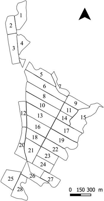
The experiment was performed in a farm in Njombe, Cameroon, during 2015 and 2016.The farm of 92 Ha consisted of 28 contiguous fields (Figure 1). Plots were planted in double rows from years 1999 to 2015. Annual rainfall in 2015 was 3074 mm and average temperature was 26.3°C. Management of the farm (irrigation, fertilization, pest control and fruits care) was done according to the conventional practices in banana farming, as well as the tagging of bunches. Indeed, each inflorescence was manually marked with a color tag at bloom. The marking was organized so that each plot was scouted twice a week. Maturity, based on finger diameter and age limit, was also assessed twice a week. The reference finger for maximum diameter was the central finger of the second hand of each bunch. The diameter limit was the same during all the experimentation.
Organization of the farm and its 28 plots.

Operators were equipped with a smartphone that they used to localize bunches when marking blooms and when assessing operational maturity. The spatial accuracy of GNSS system of smartphones was assessed to be 5 meters. Each color tag was identified by a unique bar code and a program was developed to record the time and position during scanning of tags. Finally, each bunch marked with a tag and a bar code was recorded in a database with the following attributes: date of flowering, date of operational maturity, coordinates at flowering and coordinates at operational maturity.
Data analysis and mapping
Data were processed in order to remove global outliers, such as data with wrong coordinates (i.e. outside the field borders) or faulty attribute inputs. The TFM of each bunch was then calculated as the number of days between the date of flowering and the date of operational maturity.
Following the “sample integration over time” strategy, TFM was studied over two consecutive periods P1 and P2, each period lasting 20 weeks and gathering approximately 1500 observations per hectare. P1 started on 13 October 2015 and P2 finished on 16 July 2016. Under such periods of time, the TFM of bunches of different cohorts are likely to be different due to changes in environmental conditions and to farmer’s practices that affect all the individuals of a cohort in the farm. Therefore, a measure of TFM for an individual i may be expressed as:
 $$TFM_{i} \,{\equals}\,TFM_{{cohort\left( i \right)}} {\plus}{\varepsilon}_{i} $$
where
 $$ TFM_{{cohort(i)}} $$
is the median of all the TFM corresponding to the same cohort and ε
i
is the residual. ε
i
is a centered TFM and the function ε
i
is denominated hereafter “TFMc”.
The median was preferred over the mean to estimate the cohort effect because it is less sensitive to the criterion of age limit in maturity assessment. Indeed, if A would be the probability distribution of TFM that would result of a harvest decision based only on the finger diameter, and B be the probability distribution that results from both management criteria, i.e. the finger diameter and the age limit, the mean would not be the same for the two distributions if some TFM values were affected by the age limit criterion. On the contrary, because the age limit criterion can be expected to be greater than the median of A, then the median of both distributions should be the same. The spatial variability of TFMc was quantified both at the whole farm scale and at the within field scale. In both cases all the individuals of each cohort were used to calculate TFM cohort .
The spatial variability of TFMc was quantified with an empirical omni-directional variogram (Bachmaier and Backes, Reference Bachmaier and Backes2008) as described by Bivand et al . (Reference Bivand, Pebesma and Gómez-Rubio2013). To confirm that the increase in TFMc variance with distance was not due to chance, the procedure of Bivand et al . (Reference Bivand, Pebesma and Gómez-Rubio2013) was implemented. It consists in computing variograms after randomly re-assigning measurements to spatial locations. A visually assessment is then made to check if the empirical variogram is out of the range of 95% of the simulated random variograms. All the empirical variograms at the within field scale were analyzed and represented at a maximum lag of 80 meters, corresponding to 80% of the width for most of the plots. This precaution was taken in order to prevent plot shape effects. Otherwise, very elongated plots would possibly induce a directional analysis of variance. The degree of spatial dependence of TFMc was evaluated as the proportion between the spatially correlated variance (C1) and total variance of the variogram (C0+C1). A variogram model was fitted for both periods P1 and P2 at farm scale. It was only fitted at plot scale for plots and periods where TFMc presented a spatial structure. TFMc were mapped on a square grid with 10 meters side using those theorical variograms by block kriging.
In a second step, the temporal stability of TFMc maps obtained at different periods was studied using a Spearman correlation test. This statistic was preferred over a Pearson test because of the non normality of the data. The P-value is given as an indicator but should not be used here to test statistical hypothesis because of the spatial auto-correlation of the data (Taylor and Bates, Reference Taylor and Bates2013).
Tools
Statistical tests and mapping were implemented using R (R Development Core Team, 2008) and packages gstat (Pebesma, Reference Pebesma2004) and sp (Pebesma and Bivand, Reference Pebesma and Bivand2005).
Results and discussion
Management of asynchronicity of field data
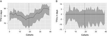
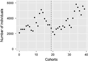
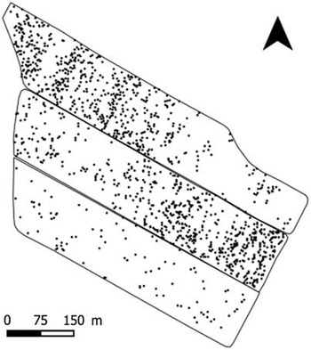
Figure 2 shows (A) the variability of TFM along cohorts and (B) the effect of centering by median. The total variance of TFM is 39 days² and the intra-cohort variance is 15 days². The number of individuals in a cohort (number of blooms per week) is variable (Figure 3). This number is particularly influenced by flowering peaks of recently planted plots which are still synchronous in the first production cycles. Moreover, as shown in Figure 4, spatial patterns of blooms can be irregular. These peculiarities of banana crops induced by asynchronicity indicate that gathering observations of several weeks will improve density and spatial repartition of the observations. They also suggest that TFMc should be analyzed, rather than TFM, in order to compensate variability due to cohorts.
(A) Time between Flowering and Maturity by cohort, (B) centered Time between Flowering and Maturity. Dotted lines correspond to the limits between Period 1 and Period 2. Lines correspond to medians and ribbons contain 95% of the values.

Variation in total number of individuals (=bunches) by cohort on the farm. Each cohort corresponds to a week.

Example of irregular repartition of blooms on plots 6, 8, 10 of week 12.

Within farm and within field variability of Time between Flowering and Maturity
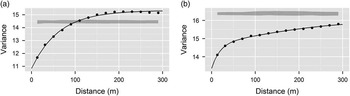
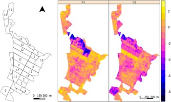
Figure 5 and 6 show respectively the variograms corresponding to period 1 and 2 and the maps resulting from the block kriging interpolation. The variograms are out of the range of 95% of the simulated random variograms indicating that the hypothesis of absence of spatial correlation is unlikely. Therefore, the degree of spatial dependence which is 0.30 at period 1 and 0.13 at period 2 is significant. The empirical variogram related to period 2 is not stationary (the variance does not reaches a plateau) which means that the spatial dependence may have a larger scale than 300 meters. Hence, the degree of spatial dependence calculated for this period may be underestimated. Differences in TFMc are visible between plots. For example, the bunches in plot 10 are mature nearly 6 days after the bunches in plots 5 or 6 during period 1. Those results highlight the spatial organization of the TFMc at the farm level, which suggests the relevance to study this indicator for precision agriculture in banana.
TFMc variograms for period 1(weeks 0 to 19) (a: P1) and period 2 (weeks 20 to 39) (b: P2) at the farm level. Ribbons envelop 95% of the variance of simulated random variograms.

Left: Map of the plots where numbers 1 and 2 mean there is respectively a spatial structure in periods 1 and 2. Right: TFMc maps (in days) obtained by block kriging.

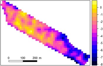
According to the variogram analyses, twelve plots present a spatial structure for both P1 and P2 periods. Among them, three plots exhibit a temporal stability in their structure (Spearman’s Rho >0.5, p-value <1.10−15). Thirteen plots exhibit a spatial structure only at period 2. The degree of spatial dependence of TFMc varies from 0% (no structure) to 25%. To strictly respect the hypothesis of stationarity required for kriging procedures, variograms should be modeled at the plot level (Figure 7).
Example of map obtained by kriging at plot level (plot 6).

Factors explaining those spatial structures in TFMc might be different according to the situation. Such factors may include biotic (e.g. black sigatoka) and abiotic (light, temperature, soil) causes as well as farm management effects (Srikul and Turner, 1995). More investigations are needed to identify the most influential factors. It is to be noted that those factors may have influenced the development of the fruit directly or indirectly by affecting the plant before bloom. Depending on the season, factors can have different effects on TFMc. The period of sample integration is a compromise between spatial resolution and time resolution of structures that are to be identified. The longer the duration of the analysis, the better the spatial resolution and the smaller the effect of spatial distribution of points, but the lower the opportunity to identify short-live phenomena.
The Nugget effect, i.e., the variance at the origin at the TFMc variogram, is important. It indicates a partial or total absence of correlation between values taken at two very close sites (Arnaud and Xavier, Reference Arnaud and Xavier2000). This can be partially explained by the lack of precision of TFM measurement method. Indeed, observations of flowering and of maturity are done twice a week. This induces a variance of around 2.5 days² in the measurements (calculation not shown), which represents 17% of the observed variability within a cohort and which is not spatially auto correlated. Moreover, the finger diameter evaluation and the tagging of fruits at bloom are done manually by operators. It can explain a part of the variability in TFM (Bugaud and Lassoudière, Reference Bugaud and Lassoudière2005). The limited spatial accuracy of the GNSS system, which is 5 meters, might also explain a part of this variability. A high proportion of the Nugget effect also comes from the intraplant variability which is not negligible.
This strong Nugget effect suggests that both the period of “sampling integration” and block size need to be carefully selected so that the number of observations is sufficient enough to increase the signal to noise ratio when kriging by block (Tisseyre et al., Reference Tisseyre, Geraudie and Saurin2015).
Conclusion
Banana production is asynchronous, which is reflected in the heterogeneity of the stages of plant development in the fields. In order to provide map of crop properties with a sufficient spatial resolution, it is necessary to normalize crop data in order to compare observations taken at different times or on different phenological status. This study illustrates the specificities of the asynchronicity that must be taken into account to produce maps of agronomic interest. A method is presented on a maturity indicator that can be interpreted as an index of vigor of fruit growth. The aim of this method is to compensate the temporal variability induced by the gathering of maturity measurement made at different dates and to create a new time-independent indicator. The spatial structure of this indicator was studied. It is spatially structured, on the scale of the farm but also of the small plots. This shows that the functioning of this culture depends on space and that precision farming approaches can be envisaged. In order to improve the agronomic interpretation of these maps so that they can serve as decision support in production, it is still necessary to identify the agronomic factors that explain the observed differences of maturity.