A) IM voltage

Nonlinear devices do not obey Ohm's law, and the nonlinear current–voltage follows the power series [Reference Henrie, Christianson and Chappell10, Reference Jiang, Li and Liu14, Reference Sui, Christensen and Durney15].

(1) $$I = f(V) = \sum\limits_{n = 1}^m {a_n V^n}, $$

where V is the voltage across the nonlinear device, I is the current through the nonlinear device, a _n (n = 1, 2, …, m) are the coefficients of the power series, and a ₃/a ₁ represents the degree of third-order PIMP.

For the two carriers, we have

(2) $$\eqalign{V &= V_1 \cos \omega _1 t + V_2 \cos \omega _2 t \cr & = \displaystyle{1 \over 2}V_1 (e^{\,j\omega _1 t} + e^{ - j\omega _1 t} ) + \displaystyle{1 \over 2}V_2 (e^{\,j\omega _2 t} + e^{ - j\omega _2 t} ) \cr &= \displaystyle{1 \over 2}(V_1 e^{\,j\omega _1 t} + V_2 e^{\,j\omega _2 t} ) + \displaystyle{1 \over 2}(V_1 e^{ - j\omega _2 t} + V_2 e^{ - j\omega _2 t} ) \cr & = \displaystyle{1 \over 2}(E + E^*),}$$

where E = V ₁ e  ^{jω ₁ t}  + V ₂ e  ^{jω ₂ t} , E* is the conjugate of E.

The binomial expansion of V ⁿ is

(3) $$\eqalign{& V^n = \displaystyle{1 \over {2^n}} (E + E^*)^n = \displaystyle{1 \over {2^n}} \sum\limits_{M_0 = 0}^n {\displaystyle{{n!} \over {M_0 !(n - M_0 )!}}} E^{n - M_0} (E^*)^{M_0},} $$

where M ₀ is the binomial variable.

The odd-order PIMP is considered because they have interference to system [Reference Eng and Stern16]. According to the binomial symmetry, equation (3) can be rewritten as

(4) $$V^n = \displaystyle{1 \over {2^n}} \left[ {2{\mathop{\rm Re}\nolimits} \sum\limits_{M_0 = 0}^{(n - 1/2)} {\displaystyle{{n!} \over {M_0 !(n - M_0 )!}}} E^{n - M_0} (E^*)^{M_0}} \right].$$

At the same way, the binomial expansions of E ^{n−M ₀} and (E*) ^{M ₀} are

(5) $$\eqalign{E^{n - M_0} &= (V_1 e^{\,j\omega _1 t} + V_2 e^{\,j\omega _2 t} )^{n - M_0} \cr &= \sum\limits_{M_1 = 0}^{n - M_0} {\displaystyle{{(n - M_0 )!} \over {M_1 !(n - M_0 - M_1 )!}}} V_1 ^{n - M_0 - M_1} V_2 ^{M_1} \cr & \quad\times \exp [j((n - M_0 - M_1 )\omega _1 + M_1 \omega _2 )t],} $$

(6) $$\eqalign{(E^*)^{M_0} &= (V_1 e^{ - j\omega _1 t} + V_2 e^{ - j\omega _2 t} )^{M_0} \cr &= \sum\limits_{M_2 = 0}^{M_0} {\displaystyle{{M_0 !} \over {M_2 !(M_0 - M_2 )!}}} V_1 ^{M_0 - M_2} V_2 ^{M_2} \cr & \quad\times \exp [ - j((M_0 - M_2 )\omega _1 + M_2 \omega _2 )t],} $$

where M ₁ and M ₂ are the binomial variables.

Substituting equations (5) and (6) into (4), the expression of V ⁿ including all frequency components is obtained as follows:

(7) $$\eqalign{V^n &= \displaystyle{1 \over {2^n}} {\mathop{\rm Re}\nolimits} \sum\limits_{M_0 = 0}^{(n - 1/2)} {\displaystyle{{n!} \over {M_0 !(n - M_0 )!}}} \cr & \quad\times \sum\limits_{M_1 = 0}^{n - M_0} {\displaystyle{{(n - M_0 )!} \over {M_1 !(n - M_0 - M_1 )!}}} V_1 ^{n - M_0 - M_1} V_2 ^{M_1} \cr & \quad\times \exp [j((n - M_0 - M_1 )\omega _1 + M_1 \omega _2 )t] \cr & \quad\times \sum\limits_{M_2 = 0}^{M_0} {\displaystyle{{M_0 !} \over {M_2 !(M_0 - M_2 )!}}} V_1 ^{M_0 - M_2} V_2 ^{M_2} \cr & \quad\times \exp [ - j((M_0 - M_2 )\omega _1 + M_2 \omega _2 )t].} $$

The above formula can be simplified as

(8) $$\eqalign{V^n &= \displaystyle{{n!} \over {2^n}} \sum\limits_{M_0 = 0}^{(n - 1/2)} {\sum\limits_{M_1 = 0}^{n - M_0} {\sum\limits_{M_2 = 0}^{M_0} {}}} \displaystyle{{V_1 ^{n - M_1 - M_2} V_2 ^{M_1 + M_2}} \over {M_1 !M_2 !(n - M_0 - M_1 )!(M_0 - M_2 )!}} \cr & \quad\times \cos [(n - 2M_0 - M_1 + M_2 )\omega _1 + (M_1 - M_2 )\omega _2 ]t.} $$

The frequency of PIMP is a linear combination of carrier frequencies, that is

(9) $$\omega _{IM} = Q\omega _1 + R\omega _2, $$

where Q and R are the arbitrary integers.

From equations (8) and (9), there are

(10) $$n - 2M_0 - M_1 + M_2 = Q,$$

(11) $$M_1 - M_2 = R.$$

From equations (10) and (11), we have

(12) $$M_0 = \displaystyle{{n - Q - R} \over 2}.$$

Substituting equations (11) and (12) into (8), we get

(13) $$\eqalign{ V^n &= \displaystyle{{n!} \over {2^n}} \sum\limits_{M_2 = 0}^{(n - Q - R/2)} {} \displaystyle{{V_1 ^{n - R - 2M_2} V_2 ^{R + 2M_2}} \over \matrix{(R + M_2 )!M_2 !(n - (n - Q - 3R/2) \hfill \cr - M_2 )!((n - Q - R/2) - M_2 )! \hfill}} \cos [Q\omega _1 + R\omega _2 ]t.} $$

According to the relationship between power and voltage,

(14) $$P = 10\log _{10} \left( {\displaystyle{{V^2} \over {2Z_0}}} \right) + 30,$$

we can derive the input voltage for the input power, where Z ₀ is the characteristic impedance.

From equation (1), we derive the analytic expression of the nth-order IM voltage as follows.

(15) $$V_{IM} = \displaystyle{{a_n} \over {a_1}} V^n. $$

Substituting equations (13) and (14) into (15), we can obtain the nth-order IM voltage.

B) PIM model of cascaded system

1) GENERAL MODEL

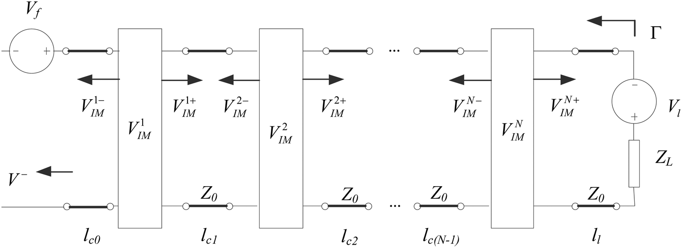
In the actual measurement, besides PIM source of microwave device under test (DUT), there are two kinds of unwanted PIM sources existing in the measurement result. One is the residual IM of measurement system, and the other is the self-interference of IM signal resulting from reflection [Reference Hienonen and Raisanen17]. Thus, the microwave network model of the cascaded system is established, as shown in Fig. 1, each DUT is regarded as a point resource.

Fig. 1.

Microwave network model of the cascaded system.

The IM distortion results from the voltage waves caused by the nonlinearities of DUT. In Fig. 1, $V_{IM}^k $ , $V_{IM}^{k +}, $ and $V_{IM}^{k -} $ represent the IM voltage, forward-propagating IM voltage and reverse-propagating (reflected) IM voltage of the kth (k = 1, 2, …, N) DUT (point source), respectively. N is the number of DUTs. The electrical length l _c0 is the distance from the first nonlinear DUT to the instrument port. The electrical length l _ck is the distance between two DUTs. The electrical length l _l is the distance from the last nonlinear DUT to the low IM load, Z _L . Z ₀ is the characteristic impedance. Γ is the reflection coefficient. V _f and V _l represent the IM voltages of instrument and load, respectively.

Assuming all PIM sources have not secondary reflection, when N = 1, the forward-propagating IM voltage is

(16) $$V_{IM}^{1 +} = V_{IM}^1. $$

If the reflected PIM measurement method is adopted, then the phase difference of signal through cable should be considered. So the reflected IM voltage is [Reference Brad and Rick6]

(17) $$V_{IM}^{1 -} = V_{IM}^1 \exp (2j\beta l_{c0} ),$$

where β is the propagation constant.

With this in mind, the reflected IM voltage, V ⁻, at the receiver, as shown in Fig. 1, is expressed as

(18) $$\eqalign{ V^ - &= V_f + V_{IM}^1 \exp [2j\beta l_{c0} ] + V_l \exp [2j\beta (l_{c0} + l_l )] \cr & \quad + \Gamma (V_f + V_{IM}^{1 +} + V_l )\exp [2j\beta (l_{c0} + l_l )].} $$

When the several DUTs are cascaded [Reference Brad and Rick6], the IM voltage can be described as

(19) $$V_{IMc}^ + = \sum\limits_{k = 1}^N {V_{IM}^k}, $$

(20) $$V_{IMc}^ - = \sum\limits_{k = 1}^N {V_{IM}^k} \exp \left[ {2j\beta \left( {\sum\limits_{s = 1}^k {l_{c(s - 1)}}} \right)} \right],$$

where $V_{IMc}^ + $ is the total forward-propagating IM voltage, $V_{IMc}^ - $ is the total reverse-propagating IM voltage.

Equation (18) can be rewritten as

(21) $$\eqalign{V^ - &= V_f + \sum\limits_{k = 1}^N {\left[ {V_{IM}^k \exp (2j\beta \left( {\sum\limits_{s = 1}^k {l_{c(s - 1)}}} \right)} \right]} \cr & \quad + V_l \exp \left[ {2j\beta \left( {\sum\limits_{k = 1}^N {l_{c(k - 1)}} + l_l} \right)} \right] \cr & \quad+ \Gamma \left( {V_f + \sum\limits_{k = 1}^N {V_{IM}^k} + V_l} \right)\exp \left[ {2j\beta \left( {\sum\limits_{k = 1}^N {l_{c(k - 1)}} + l_l} \right)} \right].} $$

Because a _n  ≪ a ₁ (n >1) in the nonlinear I–V characteristics, the impedance of point source of the kth DUT can be simplified as

(22) $$Z_{IM}^k = \displaystyle{{V^k} \over {I^k}} = \displaystyle{1 \over {a_1}}, $$

where V ^k and I ^k are the voltage and current of the kth DUT, respectively.

According to the relation between power and voltage, we derive the PIM power level as follows:

(23) $$P_{IM} = \displaystyle{{(V^ - )^2} \over {2\sum\nolimits_{k = 1}^N {Z_{IM}^k}}}. $$

Substituting equations (21) and (22) into (23), we can obtain the analytic expression of PIM power level of the cascaded system.

In order to further study PIM relationship between a single DUT and the cascaded system, equation (23) can be expanded as

(24) $$\eqalign{P_{IM} & = \displaystyle{1 \over {2\sum\nolimits_{k = 1}^N {Z_{IM}^k}}} \left( {V_f + \sum\limits_{k = 1}^N {\left( {V_{IM}^k \exp (2j\beta \left( {\sum\limits_{s = 1}^k {l_{c(s - 1)}}} \right)} \right)}} \right) \cr & \quad + V_l \exp \left( {2j\beta \left( {\sum\limits_{k = 1}^N {l_{c(k - 1)}} + l_l} \right)} \right) \cr & \quad+ \Gamma \left( {V_f + \sum\limits_{k = 1}^N {V_{IM}^k} + V_l} \right)\exp \left( {2j\beta \left( {\sum\limits_{k = 1}^N {l_{c(k - 1)}} + l_l} \right)} \right)^2 \cr & = \displaystyle{1 \over {2\sum\nolimits_{k = 1}^N {Z_{IM}^k}}} \left( {C_f^2 (V_f )^2 +\sum\limits_{k = 1}^N {C_k^2 (V_{IM}^k )^2} + C_l^2 (V_l )^2 + \Delta V^2} \right),} $$

where, C _f and C _l are the parameters of instrument and load, respectively, dependent on the phase of IM voltage. C _k is the parameters of the kth DUT dependent on the phase of IM voltage. ΔV ² is the voltage remainder. They are expressed as

(25) $$C_f = 1 + \Gamma \exp \Big(2j\beta \Big(\sum\limits_{k = 1}^N {l_{c(k - 1)}} + l_l \Big)\Big),$$

(26) $$\eqalign{& C_k = \exp \left( {2j\beta \left( {\sum\limits_{s = 1}^k {l_{c(s - 1)}}} \right)} \right) + \Gamma \exp \left( {2j\beta \left( {\sum\limits_{k = 1}^N {l_{c(k - 1)}} + l_l} \right)} \right),} $$

(27) $$C_l = (1 + \Gamma )\exp \left( {2j\beta \left( {\sum\limits_{k = 1}^N {l_{c(k - 1)}} + l_l} \right)} \right),$$

(28) $$\eqalign{ \Delta V^2 &= 2C_f C_l V_f V_l + \sum\limits_{i = 1}^N {2C_f C_i V_f V_{IM}^i }\cr &\quad+ \sum\limits_{j = 1}^N {2C_l C_j V_l V_{IM}^j} + \sum\limits_{i = 1}^{N - 1} {\sum\limits_{j = i + 1}^N {(2C_i C_j V_{IM}^i V_{IM}^j )}}.} $$

Substituting equation (23) into (24), the calculation formula of the PIM power level can be obtained as follows:

(29) $$\eqalign{P_{IM} &= \displaystyle{{C_f^2 (V_f )^2} \over {2\sum\nolimits_{k = 1}^N {Z_{IM}^k}}} + \displaystyle{{C_l^2 (V_l )^2} \over {2\sum\nolimits_{k = 1}^N {Z_{IM}^k}}} \cr & \quad+ \displaystyle{{\sum\nolimits_{k = 1}^N {C_k^2 (V_{IM}^k )^2}} \over {2\sum\nolimits_{k = 1}^N {Z_{IM}^k}}} + \displaystyle{{\Delta V^2} \over {2\sum\nolimits_{k = 1}^N {Z_{IM}^k}}} \cr & = C_f^2 P_f + C_l^2 P_l + \sum\limits_{k = 1}^N {\left( {C_k^2 P_k \cdot \displaystyle{{Z_{IM}^k} \over {\sum\nolimits_{s = 1}^N {Z_{IM}^s}}}} \right)} + \Delta P,} $$

where P _f is the PIM power level of the instrument, P _l is the PIM power level of the load, P _k is the PIM power level of the kth DUT, and ΔP is the power remainder whose expression is

(30) $$\eqalign{\Delta P &= \displaystyle{1 \over {2\sum\nolimits_{k = 1}^N {Z_{IM}^k}}} \left( {2C_f C_l V_f V_l + \sum\limits_{i = 1}^N {2C_f C_i V_f V_{IM}^i}} \right. \cr & \quad\left. { + \sum\limits_{j = 1}^N {2C_l C_j V_l V_{IM}^j} + \sum\limits_{i = 1}^{N - 1} {\sum\limits_{j = i + 1}^N {(2C_i C_j V_i V_j )}}} \right) \cr & = 2C_f C_l \sqrt {P_f P_l} + \sum\limits_{i = 1}^N {\left( {2C_f C_i \sqrt {\displaystyle{{Z_{IM}^i} \over {2\sum\nolimits_{k = 1}^N {Z_{IM}^k}}}} \sqrt {P_f P_i}} \right)} \cr & \quad+ \sum\limits_{j = 1}^N {\left( {2C_l C_j \sqrt {\displaystyle{{Z_{IM}^j} \over {2\sum\nolimits_{k = 1}^N {Z_{IM}^k}}}} \sqrt {P_l P_j}} \right)} \cr & \quad+ \sum\limits_{i = 1}^{N - 1} {\sum\limits_{j = i + 1}^N {\left( {2C_i C_j \displaystyle{{\sqrt {Z_{IM}^i Z_{IM}^j}} \over {2\sum\nolimits_{k = 1}^N {Z_{IM}^k}}} \sqrt {P_i P_j}} \right)}},} $$

where C _i and C _j are the parameters of the ith and jth DUTs, respectively, dependent on the phase of IM voltage, P _i and P _j are the PIM power levels of the ith and jth DUTs, respectively.

Equation (29) reveals the relationship of PIM power levels between a single DUT and the cascaded system. It can be seen that the PIM power level of the cascaded system nonlinearly increases with the number of cascaded DUTs.

2) SIMPLIFIED MODEL

When the nonlinear characteristics of all DUTs are nearly same, they would produce the identical PIMP under identical conditions such as same torques and working environment. Then, equations (19) and (20) can be simplified as

(31) $$V_{IMc}^ + = NV_{IM}^{}, $$

(32) $$V_{IMc}^ - = \sum\limits_{k = 1}^N {[V_{IM}} \exp (2j\beta ((k - 1)l_c + l_{c0} ))].$$

Equation (21) can be rewritten as

(33) $$\eqalign{V^ - &= V_f + \sum\limits_{k = 1}^N {[V_{IM}} \exp (2j\beta ((k - 1)l_c + l_{c0} ))] \cr & \quad+ V_l \exp [2j\beta ((N - 1)l_c + l_{c0} + l_l )] \cr & \quad + \Gamma (V_f + NV_{IM} + V_l )\exp [2j\beta ((N - 1)l_c + l_{c0} + l_l )],} $$

where l _c is the electrical length between two DUTs.

Equation (23) can be simplified as

(34) $$P_{IM} = \displaystyle{{(V^ - )^2} \over {2NZ_{IM}}}. $$

According to equations (33) and (34), PIM power levels of the cascaded system can be calculated.

Compared with the existing models, the proposed model could be applied into many situations, including the point sources and cascaded system, and considering the reflection, forward-propagation, electric length, equipment noise, etc.

A) Experimental equipment and principle

The input signal frequencies for measurement are f ₁ = 2620 MHz and f ₂ = 2690 MHz. The third-order PIMP with frequency 2f ₁ − f ₂ = 2550 MHz will be measured at room temperature.

The experimental equipment includes the Rosenberger portable PIM tester, Rosenberger low PIM load, several Pasternack N-type coaxial connectors as DUTs, and low PIM test cable with characteristic impedance of 50 Ω. The torque acting on DUTs is 10 Nm, and the measurement error of torque is 0.5 Nm.

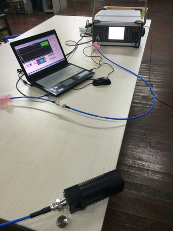
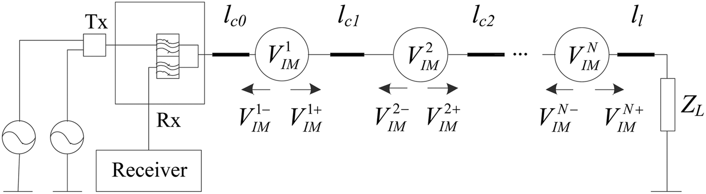
As shown in Fig. 2, the Rosenberger portable PIM tester is connected to DUT and low PIM load, the other port is connected to PC to show the results. The structure of test system is shown in Fig. 3.

Fig. 2.

Test connection diagram.

Fig. 3.

Structure of the test system.

B) Verification steps

For verifying the correctness of the proposed model, we design the following experimental verification steps:

1. (1) When P ₁ = P ₂, the third-order PIM power levels of a connector with different input powers are measured.

2. (2) When P ₁ ≠ P ₂, the third-order PIM power levels of a connector with different ratios of two input powers are measured.

3. (3) The third-order PIM power levels with different number of cascaded DUTs are measured.

4. (4) The third-order PIM power level of a single DUT is measured when P ₁ = P ₂ = 43 dBm, then a ₀ and a ₃ can be determined. Substituting a ₀ and a ₃ into equations (15) and (22), the IM voltage and impedance of point source can be acquired. Let C = n = 3, Q = 2, R = −1, l _c0 = l _l  = 1.5 m in equations (13), (14), and (33), and substituting V ₁ and V ₂ into equation (15), V _IM3 can be obtained. Finally, by equation (23) the theoretical results of third-order PIM power levels of single DUT and cascaded DUTs can be obtained.

C) Results and discussion

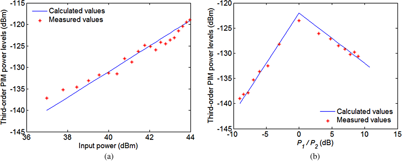
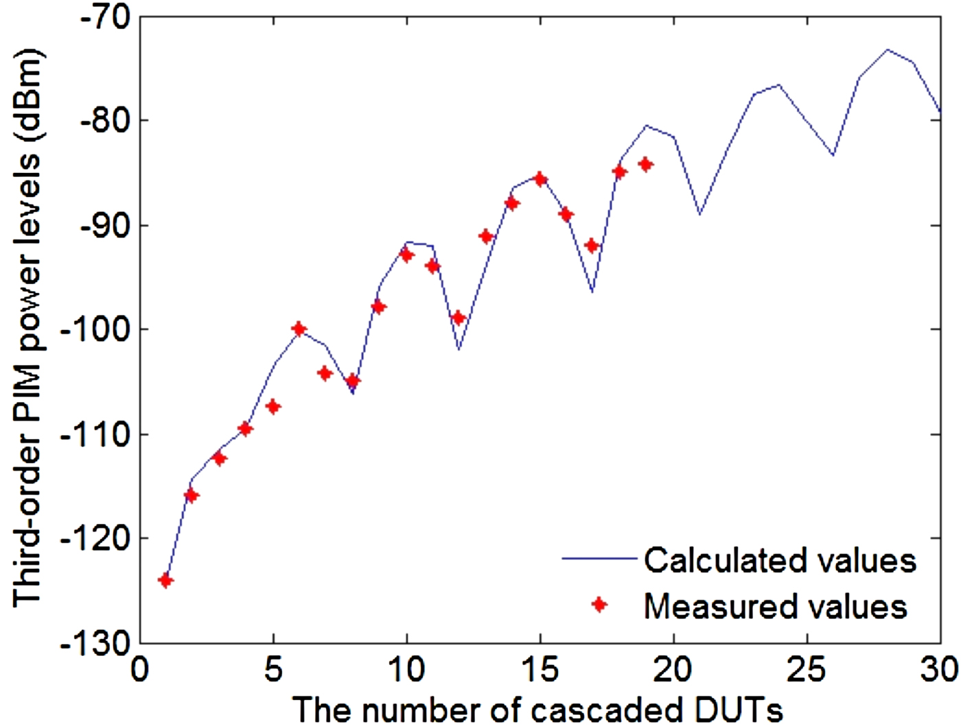
The experimental and theoretical results in different conditions are shown in Figs 4 and 5.

Fig. 4.

Comparison of the experimental and calculated values of third-order PIM power levels. (a) The third-order PIM power levels when P ₁ = P ₂. (b) The third-order PIM power levels with different ratios of two input powers.

Fig. 5.

Comparison of experimental and calculated values of third-order PIM power levels of cascaded DUTs.

As shown in Fig. 4(a), when P ₁ = P ₂ and for the different input powers, the calculated result of point-source model matches well with that of the experimental result. As shown in Fig. 4(b), when P ₁ ≠ P ₂ and for the different ratios of two input powers, the slopes of third-order PIM power levels are −1 dB and 2 dB, respectively, which can be proven as follows.

For the third-order PIM, from equations (13) and (15), there are

(35) $$V_{IM} \propto V_1^2 V_2. $$

From equations (23) and (35), the relationship between the third-order PIM power level and input powers can be obtained as

(36) $$P_{IM} \propto P_1^2 P_2. $$

Further

(37) $$P_{IM} ({\rm dBm}) \propto 30\log _{10} (P_1 ) - 10\log _{10} (P_1 /P_2 ),$$

(38) $$P_{IM} ({\rm dBm}) \propto 10\log _{10} (P_2 ) + 20\log _{10} (P_1 /P_2 ).$$

It can be seen from equation (37) that the slope of the third-order PIM power level is −1 dB, when P ₁ is constant. From equation (38) the slope of the third-order PIM power level is 2 dB, when P ₂ is constant.

The above results indicate the point-source model can accurately predict PIM power levels with different input powers.

As shown in Fig. 5, the third-order PIM power levels of different number of cascaded DUTs are measured. Although, there are some discrepancies between the experimental and calculated values because of the measurement errors among the torques acting on the cascaded DUTs, on the whole, the experimental results are consistent with the theoretical values, which indicate the cascaded model can accurately predict PIM power levels of the cascaded system. There exist some oscillations because the cascaded model considers the phase change of IM voltage.