

I. Introduction
The best way I could describe the effect of the marijuana and hashish is that it would make me relaxed and creative.Footnote 1 (Steve Jobs)
I’m not a regular smoker of weed… I don’t find that it is very good for productivity.Footnote 2 (Elon Musk)
These contrasting statements capture the persistent ambiguity surrounding the cognitive and behavioral consequences of marijuana use—ambiguity that is increasingly salient in light of ongoing policy liberalization across the United States. While public interest and macroeconomic analysis of marijuana policy have grown, the firm-level implications remain underexplored in the finance literature.
Existing empirical research offers valuable but incomplete insights. Much of it has focused on medical marijuana laws (MMLs), which apply to a narrower population and typically exert limited influence on adult-use prevalence (Cerdá, Mauro, Hamilton, Levy, Santaella-Tenorio, Hasin, Wall, Keyes, and Martins (Reference Cerdá, Mauro, Hamilton, Levy, Santaella-Tenorio, Hasin, Wall, Keyes and Martins2020)). In these contexts, access to marijuana has been shown to improve labor market outcomes by alleviating health-related employment constraints (Blake, Robson, Ho, Jubb, and McCabe (Reference Blake, Robson, Ho, Jubb and McCabe2006), Fiz, Durán, Capellà, Carbonell, and Farré (Reference Fiz, Durán, Capellà, Carbonell and Farré2011)). In contrast, recreational marijuana laws (RMLs) extend access to a broader and generally healthier working-age population, raising distinct behavioral and organizational concerns for firms. Several studies have examined the effects of RMLs on individual- or state-level labor market outcomes, often reporting null or modestly positive effects on employment, wages, or participation (Morris, TenEyck, Barnes, and Kovandzic (Reference Morris, TenEyck, Barnes and Kovandzic2014), Chakraborty, Doremus, and Stith (Reference Chakraborty, Doremus and Stith2021), and Dave, Liang, Muratori, and Sabia (Reference Dave, Liang, Muratori and Sabia2025)). However, these findings are frequently drawn from early-adopting states or narrow industry contexts, limiting their generalizability. More importantly, the literature rarely considers how firms themselves, rather than workers, respond to legalization. In this context, understanding how expanded legal access to marijuana affects corporate labor demand, investment strategy, and innovation is essential for both academic inquiry and policy design.
The legalization of recreational marijuana represents an institutional shift with complex implications for firms. On the one hand, proponents argue that RMLs stimulate economic activity by creating new jobs, expanding retail and agricultural sectors, increasing tax revenues, and reducing opioid-related harms (Bradford and Bradford (Reference Bradford and Bradford2018), Chakraborty et al. (Reference Chakraborty, Doremus and Stith2021)). They may also reduce criminal convictions and improve employment prospects for historically marginalized groups (Sabia and Nguyen (Reference Sabia and Nguyen2018)). These mechanisms may indirectly benefit firms by expanding the local labor supply, reducing hiring frictions, and improving access to marginalized talent pools. On the other hand, critics raise concerns that increased access may impair cognition, raise absenteeism, and lower productivity, particularly in cognitively demanding or safety-sensitive roles (Anderson and Rees (Reference Anderson and Rees2014), Volkow, Baler, Compton, and Weiss (Reference Volkow, Baler, Compton and Weiss2014)). Shifting workplace norms could further challenge coordination and managerial control (Anderson, Hansen, and Rees (Reference Anderson, Hansen and Rees2015), Albino (Reference Albino2017)).
This article addresses this gap by exploiting the staggered adoption of RMLs across U.S. states and implementing a difference-in-differences (DiD) framework to estimate causal impacts on firm-level employment. Recognizing the limitations of traditional two-way fixed effects (TWFE) models—particularly in the presence of heterogeneous treatment effects—I apply the imputation-based DiD estimator developed by Borusyak, Jaravel, and Spiess (Reference Borusyak, Jaravel and Spiess2024). This method constructs counterfactual outcomes using untreated firms, weighted by treatment timing and observable characteristics, to estimate the average treatment effect on the treated (ATT). The panel spans 2007–2023, covering pre- and post-legalization periods, and incorporates firm- and year-fixed effects, along with a rich set of firm- and state-level controls. To better capture geographic exposure to RMLs, this article also examines a subsample of small firms (fewer than 500 employees), which are more likely to operate within a limited regional footprint and thus be more directly affected by state-level policy changes.
The empirical findings reveal that RMLs significantly reduce firm-level employment, with the most pronounced effects emerging 3 to 4 years post-legalization. Employment trends for treated and control firms are statistically indistinguishable prior to adoption, supporting the parallel trends assumption. Economically, RMLs reduce firms’ employment growth by at least 2.7 percentage points. The results are robust to various model specifications and persist after controlling for macroeconomic conditions, the COVID-19 pandemic, and contemporaneous policy reforms.
This analysis further documents considerable heterogeneity in the impact of RMLs across firm and state characteristics. Firms with a higher proportion of high-skilled workers experience more substantial employment declines, consistent with heightened vulnerability in cognitively demanding roles. Effects are also more pronounced in unionized industries, possibly reflecting institutional rigidities that limit firms’ ability to respond to productivity shocks. Additionally, firms located in states with greater dispensary density (used as a proxy for market penetration) exhibit sharper employment reductions. Organizational culture also appears to moderate RML effects: Firms scoring highly on “respect” in culture indices, which may indicate more permissive or autonomy-oriented environments, suffer greater employment losses. These patterns suggest that internal workplace norms condition how external behavioral policies are absorbed.
In light of these findings, this article extends the analysis to explore whether RMLs influence broader dimensions of firm behavior beyond employment. Statistically significant declines are documented in capital investment, R&D expenditure, sales growth, and labor productivity following RML adoption. Consistent with the heterogeneity results—particularly those emphasizing the heightened sensitivity of high-skilled firms—innovation outcomes also deteriorate. Treated firms file fewer patents, particularly exploitative ones, receive fewer forward citations and demonstrate lower overall patent quality. These findings suggest that RMLs have wide-ranging implications, affecting not only firms’ employment levels but also their long-term growth trajectories and innovative capacities. However, no statistically significant negative effect is found on Tobin’s Q.
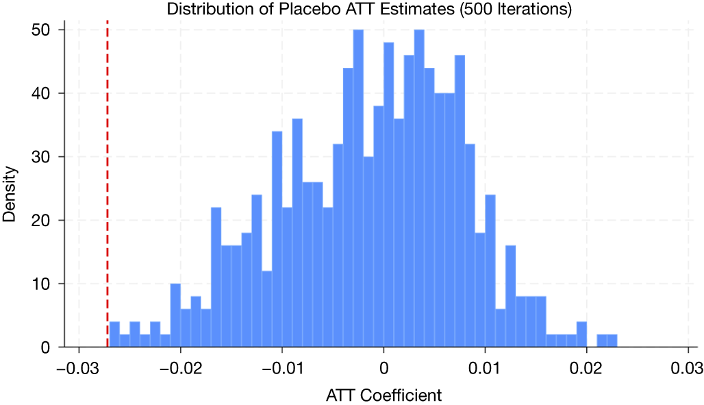
To further reinforce the credibility and specificity of the main findings, this article implements a series of placebo tests and robustness checks. First, a permutation-based falsification test is conducted by randomly assigning treatment years to RML-adopting states and reestimating the ATT 500 times. The distribution of these placebo estimates centers around zero, with none as negative as the actual treatment effect. This suggests that the observed employment effects are unlikely to be driven by chance or unrelated time trends.
In addition, this analysis assesses whether the heterogeneity results are unique to RMLs rather than artifacts of model specification. To this end, the triple differences (DDD) heterogeneity framework is replicated using placebo policies unrelated to marijuana, namely Control Share Acquisition (CSA) laws and Business Combination (BC) laws. While these corporate governance laws may influence firm behavior in other domains, they are not expected to impact employment through RML-specific channels such as marijuana exposure, unionization, or skill intensity. Using pseudo-treatment years and the same DDD specification applied in the main heterogeneity analysis, none of the placebo interaction terms are found to be statistically significant. These tests, alongside other robustness checks, including alternative sample restrictions, controls for legal confounders, and alternative operationalizations of RML exposure, collectively strengthen the conclusion that the employment and heterogeneity effects observed are specific to recreational marijuana legalization.
This article makes three key contributions to the literature on recreational marijuana legalization and corporate finance. First, this study examines the firm-level employment effects of RML, offering a new perspective distinct from the dominant focus in prior work on public health, social equity, or tax revenuesFootnote 3 (e.g., Jacobi and Sovinsky (Reference Jacobi and Sovinsky2016), Bradford and Bradford (Reference Bradford and Bradford2018), Brinkman and Mok-Lamme (Reference Brinkman and Mok-Lamme2019), Hansen, Miller, and Weber (Reference Hansen, Miller and Weber2020), Mace, Patel, and Seegert (Reference Mace, Patel and Seegert2020), Hollenbeck and Uetake (Reference Hollenbeck and Uetake2021), Sabia, Dave, Alotaibi, and Rees (Reference Sabia, Dave, Alotaibi and Rees2021), (Reference Sabia, Dave, Alotaibi and Rees2024), Auriol, Mesnard, and Perrault (Reference Auriol, Mesnard and Perrault2023), Cheng, De Franco, and Lin (Reference Cheng, De Franco and Lin2023), Mathur and Ruhm (Reference Mathur and Ruhm2023), Dave et al. (Reference Dave, Liang, Muratori and Sabia2025), and Guernsey, Serfling, and Yan (Reference Guernsey, Serfling and Yan2025)). While several studies have explored the aggregate labor market or state-level effects of marijuana laws (e.g., Anderson and Rees (Reference Anderson and Rees2014), Morris et al. (Reference Morris, TenEyck, Barnes and Kovandzic2014), Dave et al. (Reference Dave, Liang, Muratori and Sabia2025)), this article focuses on the firm as the unit of decision-making, where hiring, investment, and employment structures are determined.
In particular, this analysis complements recent finance-oriented work on marijuana legalization. Guernsey et al. (Reference Guernsey, Serfling and Yan2025), for instance, show that MMLs decrease firms’ cost of equity and thus reduce labor market risk, while Cheng et al. (Reference Cheng, De Franco and Lin2023) show that the passage of MMLs is associated with higher state bond spreads. These studies highlight the informational and market-pricing consequences of marijuana liberalization. In contrast, this study focuses on firms’ internal, real-side adjustments—particularly those involving human capital and innovation. By isolating the effect of RMLs on corporate hiring, especially in firms with high exposure to marijuana-related frictions, this article provides novel evidence on how behavioral policy reforms manifest as organizational frictions. Crucially, the findings suggest that the consequences of marijuana legalization extend beyond the marijuana industry, highlighting significant spillover effects on labor, innovation, and productivity across a wide range of firms.
Second, this study contributes to the growing literature on labor market frictions and firm behavior, which examines the interplay between labor market frictions and firm performance (e.g., Atanassov and Kim (Reference Atanassov and Kim2009), Boustanifar (Reference Boustanifar2014), Belo, Lin, and Bazdresch (Reference Belo, Lin and Bazdresch2014), Donangelo (Reference Donangelo2014), Giroud and Mueller (Reference Giroud and Mueller2015), Belo, Li, Lin, and Zhao (Reference Belo, Li, Lin and Zhao2017), Kuehn, Simutin, and Wang (Reference Kuehn, Simutin and Wang2017), Donangelo, Gourio, Kehrig, and Palacios (Reference Donangelo, Gourio, Kehrig and Palacios2019), Benmelech, Bergman, and Seru (Reference Benmelech, Bergman and Seru2021), and Nishesh, Ouimet, and Simintzi (Reference Nishesh, Ouimet, Simintzi and Denis2024)), by identifying a new, policy-driven source of friction: the legalization of recreational substances. The findings show that RMLs induce frictions in workforce management, particularly in firms with high-skilled labor, strong union presence, or tolerant corporate cultures. These frictions manifest in reduced employment, lower productivity, and ultimately dampened firm investment and innovation. In this way, this article extends recent work on the financial consequences of health-related societal shocks, such as the opioid crisis. Cornaggia, Hund, Nguyen, and Ye (Reference Cornaggia, Hund, Nguyen and Ye2022) demonstrate that opioid misuse imposes fiscal costs via increased mortality and social disruption, Ouimet, Simintzi, and Ye (Reference Ouimet, Simintzi and Ye2025) observe a negative effect of opioid prescriptions on subsequent individual employment, and Jansen (Reference Jansen2023) shows that the opioid epidemic generates negative spillovers in household credit and consumption through increases in loan defaults. This study complements this literature by showing that even state-sanctioned behavioral liberalization—rather than public health deterioration—can have unintended adverse effects on firms.
Third, this article contributes to the broader literature linking legal institutions and behavioral regulation to corporate outcomes. While much of the existing research—including seminal works by La Porta, Lopez-de-Silanes, Shleifer, and Vishny (Reference La Porta, Lopez-de-Silanes, Shleifer and Vishny1998), Bertrand and Mullainathan (Reference Bertrand and Mullainathan2003), Bhattacharya and Daouk (Reference Bhattacharya and Daouk2009), Francis, Hasan, John, and Waisman (Reference Francis, Hasan, John and Waisman2010), Serfling (Reference Serfling2016), Karpoff and Wittry (Reference Karpoff and Wittry2018), Chava, Danis, and Hsu (Reference Chava, Danis and Hsu2020), Frattaroli (Reference Frattaroli2020), Gao, Hsu, Li, and Zhang (Reference Gao, Hsu, Li and Zhang2020), and Olson, Yust, and Christensen (Reference Olson, Yust and Christensen2023)—examines how legal institutions and regulatory constraints shape firm behavior, this study focuses on the economic consequences of marijuana legalization. Building on this body of research, this analysis examines how such legal changes affect both innovation outcomes and employment dynamics.
In contrast to Gao et al. (Reference Gao, Hsu, Li and Zhang2020) and Olson et al. (Reference Olson, Yust and Christensen2023), who find that smoking bans enhance innovation by modifying employee behavior and workplace dynamics, this article investigates the effects of relaxing behavioral constraints. Despite the opposing directions of these interventions—restriction versus liberalization—this analysis finds comparable magnitudes of effect. Importantly, this study builds on these prior studies by explicitly controlling for the presence of smoking bans at the state level. This allows the analysis to isolate the effect of marijuana legalization from other cooccurring public health policies. Even after accounting for these existing restrictions, this article finds that firms exposed to RMLs experience significant declines in both exploitative and exploratory patenting, forward citations, and overall patent quality, alongside adverse shifts in employment dynamics. The findings suggest that liberalization can be as impactful as restriction, not only in shaping innovation outcomes but also in influencing workforce structure and labor market responses—albeit with potentially negative consequences. This suggests that RMLs introduce a distinct channel of behavioral friction—possibly related to changes in cognitive performance, absenteeism, or workplace norms—that extends beyond the mechanisms identified in the smoking ban literature. In this way, this article broadens the scope of the law-and-finance literature by demonstrating that socially motivated, noncorporate policies can have substantial spillover effects on firm operations and strategic decision-making. These results underscore the importance of incorporating the wider institutional and behavioral environment into corporate finance research.
The structure of the article is organized as follows: Section II introduces the institutional background of marijuana legalization, Section III outlines the identification strategy and data, Section IV presents the main empirical findings, and Section V concludes.
II. Institutional Background
The legal status of marijuana in the United States has undergone substantial transformation over the past century, marked by shifting regulatory frameworks at both the federal and state levels. In the late 19th century, industrial hemp was widely cultivated—particularly in states such as Kentucky—playing a significant role in the agricultural economy (United States Bureau of the Census (1913)). However, the early 20th century saw growing societal and political opposition to marijuana, resulting in the introduction of state-level prohibitions during the 1910s. These efforts culminated in federal restrictions through key legislative interventions, including the Uniform State Narcotic Drug Act of 1935 and the Marihuana Tax Act of 1937. The latter imposed taxation and stringent regulatory controls on the importation, cultivation, possession, and distribution of marijuana, with violations subject to fines and imprisonment (Sabia and Nguyen (Reference Sabia and Nguyen2018)).
A temporary revival in hemp production occurred during the Second World War, driven by material shortages that necessitated increased domestic sourcing (Johnson (Reference Johnson2014), Hudak (Reference Hudak2018)). Nevertheless, following the war, marijuana remained tightly regulated. In 1970, federal prohibition was further reinforced by the Controlled Substances Act, which classified marijuana as a Schedule I substance—indicating a high potential for abuse and no recognized medical application—thereby rendering it illegal under federal law nationwide.
Despite this enduring federal stance, state-level challenges to prohibition gradually emerged. California led this shift in 1996 by enacting Proposition 215—the Compassionate Use Act—which legalized medical marijuana (National Conference of State Legislatures (2020)). This landmark legislation catalyzed further state-level reforms and signaled a pivotal change in policy direction. The shift was further solidified by the U.S. Department of Justice’s 2009 memorandum, which advised federal prosecutors to deprioritize enforcement against individuals and businesses operating in compliance with state MML. This federal guidance contributed to increased legitimacy and investment in the nascent marijuana industry (Stout and Moore (Reference Stout and Moore2009)).
The momentum toward legalization accelerated markedly in 2012, when Colorado and Washington became the first states to approve recreational marijuana use through ballot initiatives. Since then, the legal marijuana market has expanded rapidly. By the end of 2023, 39 states and the District of Columbia had legalized medical marijuana, while 24 of those states—plus the District—had also legalized recreational use (as illustrated in Figure 1). The timelines for implementing recreational sales vary widely across jurisdictions, ranging from under 3 months in Arizona to up to 4 years in Maine. On average, states experienced an implementation lag of approximately 16 months (Ward (Reference Ward2022)).
Figure 1 presents a choropleth map of the United States illustrating the legal status of marijuana at the state level. States are categorized into two groups: i) states with legalized medical marijuana only (depicted in light green), and ii) states with both legalized medical and recreational marijuana (depicted in dark green). States shown in white/grey indicate jurisdictions where marijuana remains prohibited in both forms. Source: ProCon.org at https://marijuana.procon.org/legal-recreational-marijuana-states-and-dc/.

Figure 1 Long description
A map of the United States uses three colors to categorize marijuana laws.
Dark green represents states with both legalized medical and recreational marijuana. These are concentrated in the West including W A, O R, C A, N V, A Z, M T, C O, and N M. In the Midwest and East, this includes M N, I L, M O, M I, O H, V A, N Y, M E, and the non-contiguous state of A K.
Light green represents states with legalized medical marijuana only. These are distributed across the central and eastern regions including N D, S D, U T, O K, A R, L A, M S, A L, F L, K Y, W V, P A, N H, and the non-contiguous state of H I.
White or light grey represents states where marijuana remains prohibited in both forms. This includes a central corridor of I D, W Y, N E, K S, and T X, as well as I A, W I, I N, T N, N C, S C, G A, and several small Northeastern states including V T, M A, R I, C T, N J, D E, M D, and D C.
In parallel, numerous states have adopted partial reforms, including the decriminalization of small-scale possession and the legalization of low-Δ⁹-tetrahydrocannabinol (THC) cannabidiol (CBD) for medical purposes. These legal changes reflect a broader societal shift in attitudes toward marijuana. According to recent surveys, a record high 68% of Americans now support legalization—up from approximately 50% a decade earlier (Gallup (2025)).Footnote 4 This shift in public sentiment suggests continued momentum for reform, with many states actively considering new legalization or ballot measures concerning both medical and recreational marijuana use.
III. Data and Empirical Approach
A. Empirical Approach
I exploit the staggered adoption of recreational marijuana legalization across U.S. states within a DiD framework, initially employing a TWFE specification. The key identification assumption is that firms located in states yet to legalize recreational marijuana serve as valid counterfactuals for treated firms, conditional on observable and time-invariant unobserved factors.
The baseline specification is defined as follows:

where i denotes the firm, s the state, and t the year.
$ {Employment}_{i,s,t} $
 is defined as the annual change in the number of employees for firm i in state s at year t.
$ {Treat}_s $
 equals to 1 when a firm is headquartered in a state that has legalized recreational marijuana by year t, and 0 otherwise.
$ {Post}_t $
 corresponds to a dummy that is set to 1 for years after the state legalized recreational marijuana, and to 0 otherwise.
$ {\beta}_1 $
 indicates primary interest in this regression. If marijuana legalization matters for a firm’s employment, then
$ {\beta}_1 $
 should be significantly different from 0. I cluster standard errors by state to account for serial correlation in the standard errors within a firm over time and across firms within the same state.
$ {X}_{i,\mathrm{s},t} $
 represents a set of control variables that account for firm-specific characteristics. Building on established literature (e.g., Ellul, Pagano, and Schivardi (Reference Ellul, Pagano and Schivardi2018), Ersahin and Irani (Reference Ersahin and Irani2020), Benmelech et al. (Reference Benmelech, Bergman and Seru2021), and Peng, Shi, and Yu (Reference Peng, Shi and Yu2025)), I incorporate controls for key firm-level variables such as leverage, Tobin’s Q, cash flow, size, return on assets (ROA), capital investment (CAPX/AT), and sales growth.
$ {Z}_{s,t} $
 represents state-level factors, including the gross state product (GSP) growth rate, unemployment rate, government spending-to-GSP ratio, taxation freedom, labor market freedom, and state-level economic policy uncertainty (EPU), capturing broader macroeconomic conditions. I also consider whether the headquarters state is a blue state, whether it is incorporated in Delaware, whether it bans smoking in public places, and whether it adopts right-to-work (RTW) laws, as each of these factors may influence corporate decisions (e.g., Daines (Reference Daines2001), Chava et al. (Reference Chava, Danis and Hsu2020), and Gao et al. (Reference Gao, Hsu, Li and Zhang2020)). Each of these policy controls is specified as an indicator variable that equals 0 prior to the policy’s enactment, and 1 in all subsequent years. Moreover, I include firm-fixed effects (
$ {\varphi}_i $
 ) to capture the time-invariant firm-specific characteristics, while year-fixed effects (
$ {\vartheta}_t $
 ) reflect the unobserved heterogeneity that varies across time.
A key consideration in the main analysis is the geographic dispersion of a firm’s workforce. For example, although Starbucks is headquartered in Seattle, WA, most of its employees work outside Washington. In such cases, identifying the “relevant” location that influences a firm’s employment decisions following regulatory changes can be challenging, potentially affecting the estimates. To address this concern, rather than relying solely on the full sample, I also focus on smaller firms that are more likely to have the majority of their workforce concentrated at their headquarters. This approach helps ensure that the main identification strategy more accurately reflects the intended geographic dimension of treatment.
Regarding the estimation method, TWFE models can introduce biases in staggered DiD frameworks due to assumptions about homogeneous treatment effects and variations in treatment timing. These biases emerge when treatment effects evolve over time or when units treated later serve as controls for those treated earlier, potentially leading to distorted results (Callaway and Sant’Anna (Reference Callaway and Sant’Anna2021), Goodman-Bacon (Reference Goodman-Bacon2021), Baker, Larcker, and Wang (Reference Baker, Larcker and Wang2022a), and Borusyak et al. (Reference Borusyak, Jaravel and Spiess2024)). To mitigate these issues, I employ the imputation-based approach proposed by Borusyak et al. (Reference Borusyak, Jaravel and Spiess2024), which effectively addresses heterogeneity in treatment effects and the timing of treatment.
This imputation-based method offers several advantages: It is transparent, exhibits favorable efficiency properties, and allows for the estimation of asymptotically conservative standard errors. The method enhances the precision of causal estimates by constructing a counterfactual employment trajectory for firms not exposed to marijuana legalization, using the control group to predict employment dynamics in the absence of RML. It accounts for both firm-specific and time-specific factors and then imputes what the employment levels would have been for treated firms during the post-legalization period, assuming they had not been affected by RML adoption. The causal effect of RML is estimated by comparing the imputed employment levels with the observed levels in the treated group. These estimates are subsequently aggregated and weighted to calculate the average treatment effect.
B. Data and Summary Statistics
The primary sample comprises data spanning from 2007 to 2023. I initiated the analysis in 2007 to establish pre-RML trends before the first RML laws were enacted by Washington and Colorado in 2012. For data on state marijuana laws, I rely on ProCon.org, a nonprofit, nonpartisan public charity. ProCon.org provides a comprehensive analysis of the pros, cons, and supporting research on over 80 controversial issues, including state propositions and bills related to marijuana legislation. Previous studies (e.g., Chu and Townsend (Reference Chu and Townsend2019), Cheng et al. (Reference Cheng, De Franco and Lin2023)) have utilized this data to examine the impacts of marijuana laws. I further verify the accuracy of the data by cross-referencing the dates with those listed on official state legislature websites. Table 1 shows the recreational marijuana legalization dates by states.

Table 1 Long description
The table contains four columns: State, Passed Year, Effective Year, and Legalization Method. It lists the following data for states that have legalized recreational marijuana:
* Alaska: Passed 2014, Effective 2015, Initiated ballot measure.
* Arizona: Passed 2020, Effective 2020, Initiated ballot measure.
* California: Passed 2016, Effective 2016, Initiated ballot measure.
* Colorado: Passed 2012, Effective 2012, Initiated ballot measure.
* Connecticut: Passed 2021, Effective 2021, Legislative bill.
* Delaware: Passed 2023, Effective 2023, Legislative bill.
* Illinois: Passed 2019, Effective 2020, Legislative bill.
* Maine: Passed 2016, Effective 2017, Initiated ballot measure.
* Maryland: Passed 2022, Effective 2023, Legislatively referred ballot measure.
* Massachusetts: Passed 2016, Effective 2016, Initiated ballot measure.
* Michigan: Passed 2018, Effective 2018, Initiated ballot measure.
* Minnesota: Passed 2023, Effective 2023, Legislative bill.
* Missouri: Passed 2022, Effective 2022, Initiated ballot measure.
* Montana: Passed 2020, Effective 2021, Initiated ballot measure.
* Nevada: Passed 2016, Effective 2017, Initiated ballot measure.
* New Jersey: Passed 2020, Effective 2021, Legislatively referred ballot measure.
* New Mexico: Passed 2021, Effective 2021, Legislative bill.
* New York: Passed 2021, Effective 2021, Legislative bill.
* Ohio: Passed 2023, Effective 2023, Initiated ballot measure.
* Oregon: Passed 2014, Effective 2015, Initiated ballot measure.
* Rhode Island: Passed 2022, Effective 2022, Legislative bill.
* Vermont: Passed 2018, Effective 2018, Legislative bill.
* Virginia: Passed 2021, Effective 2021, Legislative bill.
* Washington: Passed 2012, Effective 2012, Initiated ballot measure.
States listed without data include Alabama, Arkansas, Florida, Georgia, Hawaii, Idaho, Indiana, Iowa, Kansas, Kentucky, Louisiana, Mississippi, Nebraska, New Hampshire, North Carolina, North Dakota, Oklahoma, Pennsylvania, South Carolina, South Dakota, Tennessee, Texas, Utah, West Virginia, Wisconsin, and Wyoming.
This study employs annual firm-level data from the Compustat database, with employment defined as the annual change in the number of employees (Ellul et al. (Reference Ellul, Pagano and Schivardi2018), Benmelech, Frydman, and Papanikolaou (Reference Benmelech, Frydman and Papanikolaou2019)). Building on established literature (e.g., Ellul et al. (Reference Ellul, Pagano and Schivardi2018), Benmelech et al. (Reference Benmelech, Frydman and Papanikolaou2019), Ersahin and Irani (Reference Ersahin and Irani2020), and Peng et al. (Reference Peng, Shi and Yu2025)), I incorporate controls for key firm-level variables such as leverage, Tobin’s Q, cash flow, size, ROA, capital investment (CAPX/AT), and sales growth. These variables provide a comprehensive view of the firms’ financial performance and investment capacity. Detailed descriptions of these variables are provided in the Appendix.
I also incorporate various macroeconomic indicators, including GSP growth from the U.S. Bureau of Economic Analysis (BEA), the unemployment rate from the U.S. Bureau of Labor Statistics, and the state-level EPU index from Baker, Davis, and Levy (Reference Baker, Davis and Levy2022b). Data on fiscal measures, specifically government spending scaled by GSP, are sourced from the State and Local Finance Initiative at the Urban Institute. Additionally, indicators of taxation freedom and labor market freedom are obtained from the Fraser Institute.Footnote 5 Taxation freedom measures the tax burden, with higher scores reflecting regions with lower, less restrictive taxes. Labor market freedom evaluates flexibility in hiring, firing, and regulatory constraints, awarding higher scores to regions with fewer restrictions. The analysis also includes data on RTW laws and public smoking bans, drawn from previous studies (e.g., Chava et al. (Reference Chava, Danis and Hsu2020), Gao et al. (Reference Gao, Hsu, Li and Zhang2020)) and state-level legislative websites.
I require firms to have complete data available for all variables used in the baseline regression, ensuring that each firm includes observations for all firm-level and dependent variables. The sample period spans from 2007 to 2023, covering 5 years before the first state legalized recreational marijuana in 2012.Footnote 6 Since this article needs to determine whether a firm is subject to RML based on its headquarters’ state, the first step is to identify the firm’s headquarters location. However, Compustat only provides information on the most recent headquarters state, which may introduce measurement errors since firms can change their headquarters. To address this, this article follows Bai, Fairhurst, and Serfling (Reference Bai, Fairhurst and Serfling2020) and Gao, Leung, and Qiu (Reference Gao, Leung and Qiu2021) and uses SEC filings from EDGAR to identify each firm’s headquarters. To prevent extreme values from skewing the analysis, all nonbinary firm-level and state-level variables are winsorized at the 1% level. Table 2 presents summary statistics for the primary variables, comprising nonmissing data across 57,070 observations.

Table 2 Long description
The table contains six columns: Variable, N, Mean, Std. Dev., Min, and Max. All variables have an N of 57,070.
* Employment: Mean 0.0661, Std. Dev. 0.3198, Min -0.6667, Max 1.8919.
* Tobin's Q: Mean 3.2759, Std. Dev. 13.7802, Min -7.9438, Max 175.2135.
* Cash flow: Mean -0.4132, Std. Dev. 2.4335, Min -23.8333, Max 0.4541.
* Leverage: Mean 1.0868, Std. Dev. 3.4797, Min 0.0263, Max 34.1142.
* R O A: Mean -0.2779, Std. Dev. 1.8070, Min -17.5641, Max 0.4570.
* C A P X / A T: Mean 0.0383, Std. Dev. 0.0571, Min 0.0000, Max 0.3623.
* Size: Mean 6.0706, Std. Dev. 2.6156, Min 0.0060, Max 11.8285.
* Sales growth: Mean 0.2000, Std. Dev. 0.5596, Min -0.8476, Max 2.8857.
* G S P growth: Mean 3.9840, Std. Dev. 3.4461, Min -4.6000, Max 13.7000.
* Unemployment: Mean 2.4596, Std. Dev. 1.7635, Min 0.4333, Max 8.0583.
* Government spending: Mean 13.3815, Std. Dev. 2.1867, Min 9.4452, Max 19.3650.
* E P U (log): Mean 5.1603, Std. Dev. 0.4130, Min 4.1654, Max 6.4779.
* Taxation freedom: Mean 5.4967, Std. Dev. 1.2192, Min 2.8755, Max 8.4182.
* Labor market freedom: Mean 6.0138, Std. Dev. 1.0110, Min 3.3601, Max 8.4072.
* Blue state: Mean 0.4583, Std. Dev. 0.4983, Min 0.0000, Max 1.0000.
* Smoking ban: Mean 0.7616, Std. Dev. 0.4261, Min 0.0000, Max 1.0000.
* Right to work (R T W): Mean 0.3736, Std. Dev. 0.4838, Min 0.0000, Max 1.0000.
* Delaware: Mean 0.5991, Std. Dev. 0.4901, Min 0.0000, Max 1.0000.
On average, firms report an employment growth rate of 6.61%. Tobin’s Q, a measure of firm valuation, has a mean of 3.2759, suggesting moderate market valuation relative to firm assets. In contrast, cash flow exhibits a negative mean of −0.4132, indicating that, on average, firms in the sample experience negative cash flow. The sales growth rate averages 20%, reflecting a moderate increase in sales. Firm leverage has a relatively high mean of 1.0868, signifying a substantial reliance on debt financing. The average firm size, as measured by the natural logarithm of total assets, is 6.0706. Additionally, the capital investment rate (CAPX/AT) averages 3.83%, while ROA is negative, with a mean of −0.2779.
From a state-level perspective, the average GSP growth rate is 3.98%, indicating moderate economic growth across regions. The average unemployment rate stands at 2.46%, while government spending accounts for 13.38% of GSP. The EPU index—log-transformed for scaling—has a mean value of 5.16, suggesting a moderate level of policy uncertainty during the sample period. On average, the taxation freedom score is around 5.50, and the labor market freedom scores about 6.01. Within the sample, 45.8% of states are classified as typically “blue,” indicating general support for the Democratic Party. Approximately 37.4% have enacted RTW laws, 76.2% have implemented state-level smoking bans, and 59.9% are incorporated in Delaware.
IV. Empirical Results
A. Baseline Results
Table 3 presents the baseline results analyzing the impact of RML adoption on firm-level employment.Footnote 7 Across all model specifications, the findings consistently indicate a reduction in employment following RML adoption. In the initial specification (column 1), which includes only firm- and year-fixed effects, RML adoption is associated with a statistically significant negative effect on employment growth, corresponding to a 2.78 percentage point decline. In column 2, after controlling for Tobin’s Q and cash flow, the negative association between RML adoption and employment persists, with the estimated coefficient remaining statistically significant at −0.0274.

Table 3 Long description
The table displays regression coefficients for the dependent variable Employment across four numbered columns (1 to 4).
Panel A: Full Sample (57,070 observations).
* Post times Treat: Coefficients range from -0.0272 to -0.0300, all significant at the 1 percent level. Standard errors are approximately 0.0075 to 0.0079.
* Treat: Coefficients range from -0.017 to -0.0268, none are statistically significant.
* Control variables: Cash flow, Tobin’s Q, Sales growth, C A P X / A T, R O A, Size, and Leverage are added sequentially in models 2 and 3. Most are significant at the 1 percent level except R O A and Leverage.
* State-level controls: G S P growth, Unemployment rate, and Right to work are significant in model 4.
* Fixed Effects: All models include Firm F E and Year F E.
Panel B: Small Firm Sample (25,220 observations).
* Post times Treat: Coefficients range from -0.0344 to -0.0485, significant at the 1 percent level in models 1-3 and 5 percent level in model 4.
* Treat: Coefficients range from -0.0171 to -0.0288, none are statistically significant.
* Control variables: Similar patterns to Panel A, with C A P X / A T showing a higher coefficient of 0.5439 in model 4.
* Fixed Effects: All models include Firm F E and Year F E.
Column 3 extends the analysis by incorporating additional firm-level control variables, where the interaction term (Post × Treat) continues to exhibit a significantly negative coefficient, suggesting an even stronger effect with a coefficient of −0.03. In column 4, after accounting for state-level macroeconomic and institutional variables, the results remain robust, indicating that the negative impact of RML adoption on employment is not attributable to broader economic conditions. From an economic perspective, the most conservative estimates indicate that employment growth decreases by −0.0272, corresponding to an approximate 2.72 percentage point reduction in employment growth.
To account for geographic dispersion in workforce allocation, I follow the U.S. Small Business Administration’s definition and restrict the sample to firms with 500 or fewer employees (Acs and Audretsch (Reference Acs and Audretsch1988), Autor, Cho, Crane, Goldar, Lutz, Montes, Peterman, Ratner, Villar, and Yildirmaz (Reference Autor, Cho, Crane, Goldar, Lutz, Montes, Peterman, Ratner, Villar and Yildirmaz2022)). This subsample, reported in Panel B of Table 3, reveals even stronger effects: Across all model variants, RML adoption leads to a reduction in employment growth of at least 3.44 percentage points. These results underscore the heightened sensitivity of smaller, geographically concentrated firms to labor market frictions induced by policy changes.
B. Dynamic Relationships
To address potential concerns regarding endogeneity and reverse causality, I adopt the approach of Bertrand and Mullainathan (Reference Bertrand and Mullainathan2003) and Nunn and Qian (Reference Nunn and Qian2011), placing particular emphasis on the timing of employment changes relative to the adoption of RML. This method can assess whether pretreatment trends in employment may bias the DiD estimates by violating the parallel trends assumption. If reverse causality were present, one would expect to observe a noticeable trend in employment prior to the adoption of marijuana legalization.
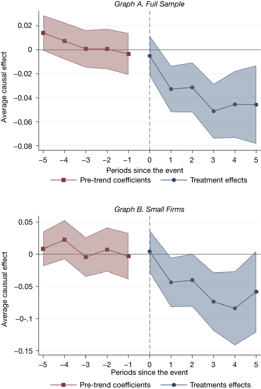
Figure 2 presents employment trends across the pre- and post-RML adoption periods. Graph A displays results for the full sample, while Graph B focuses on the subsample of small firms. Several important insights emerge. First, prior to RML adoption, there are no statistically significant differences in employment trends between the treated and control groups. This finding supports the validity of the parallel trends assumption, as both groups exhibit similar employment trajectories prior to legalization. Second, the estimated coefficients for RML are generally close to 0 and statistically insignificant in the pre-adoption period, but become significantly negative following legalization. This pattern lends support to the hypothesis that the observed decline in employment among treated firms is attributable to RML adoption, rather than to unobserved confounding factors. Third, the post-legalization period reveals a pronounced and statistically significant decline in employment within the treated group, with the effect becoming evident approximately 1 year after adoption and peaking between 3 and 4 years thereafter. This delayed response is intuitive, as firms may require time to adjust their organizational and employment structures in response to the evolving regulatory environment. The most substantial effects are observed in the fourth year following legalization, potentially reflecting the time required for marijuana markets to mature and for firms to adapt to the new economic and institutional landscape.
In Figure 2, I plot the coefficients of RMLs for corporate employment using equation (1). The horizontal axis represents the timeline, spanning from 5 years before the passage of RMLs to 5 years after their completion. The vertical axis illustrates the difference in employment between the treated and control groups. A 5% confidence interval is reported.

Figure 2 Long description
The image contains two vertically stacked line graphs, Graph A and Graph B. Both share the same X-axis labeled Periods since the event, ranging from minus 5 to 5, and a Y-axis labeled Average causal effect. A vertical dashed line at zero marks the event passage.
* Graph A. Full Sample. The Y-axis ranges from minus 0.08 to 0.02. To the left of the event, Pre-trend coefficients marked with red squares show a slight downward trend from 0.015 at minus 5 to near zero at minus 1, with a shaded 95% confidence interval. To the right of the event, Treatment effects marked with blue circles show a sharp decline, starting near zero at period 0 and dropping to approximately minus 0.05 by period 3, remaining stable through period 5. The blue shaded confidence interval widens over time.
* Graph B. Small Firms. The Y-axis ranges from minus 0.15 to 0.05. Pre-trend coefficients fluctuate around the zero line between minus 5 and minus 1. Post-event Treatment effects show a more pronounced negative trend than the full sample, dropping from zero at period 0 to a low of nearly minus 0.08 at period 4, before a slight uptick at period 5. The blue shaded confidence interval is significantly wider than in Graph A, indicating higher variance.
These findings reinforce the credibility of the identification strategy and underscore the robustness of the estimated negative employment effect. Taken together, Table 3 and Figure 2 provide compelling evidence that the adoption of RML exerts a meaningful and persistent dampening effect on firm-level employment growth.
C. Heterogeneity Analysis
Having established a systematic decline in employment following RML adoption across the overall sample, I now extend the analysis by examining heterogeneity across firms. I hypothesize that the impact of marijuana legalization on employment is likely to vary according to the range of potential outcomes and the likelihood of policy-related shocks. Accordingly, I anticipate differences in the magnitude of employment changes across various firm- and region-level characteristics.Footnote 8
1. High Skilled Versus Less Skilled Labor
The heterogeneity analysis begins by examining whether the employment effects of RML differ by the skill composition of a firm’s workforce. Exploring whether RML has a greater effect on firms employing skilled or less-skilled labor is essential, given plausible arguments supporting both scenarios. Firms with skilled labor may experience stronger negative effects, as these positions demand high levels of cognitive function, precision, and responsibility. Impairments resulting from increased marijuana use could lead to significant productivity losses and safety concerns, prompting firms to enforce strict drug policies and potentially reduce employment (Volkow et al. (Reference Volkow, Baler, Compton and Weiss2014)). Conversely, firms employing less-skilled labor might face a higher prevalence of marijuana use among employees, leading to increased absenteeism, reduced productivity, and higher turnover rates (Kaestner (Reference Kaestner1991)). These challenges could also result in employment reductions as firms strive to maintain operational efficiency.
Given the credible reasons for both types of firms to be adversely affected by RML, it is worthwhile to conduct an empirical investigation to determine which group experiences a more significant impact. Understanding the differential effects will provide valuable insights for policymakers and business leaders to develop targeted strategies that address the specific needs and vulnerabilities of each sector (DeSimone (Reference DeSimone2002)). This analysis not only contributes to the academic discourse on labor market dynamics but also informs practical approaches to mitigate the potential negative consequences of RML on employment across different segments of the workforce.
To assess these differential effects, we categorize firms based on the skill intensity of their respective industries, using the classification proposed by Belo et al. (Reference Belo, Li, Lin and Zhao2017). An industry is defined as high skilled if more than 50% of its workforce is employed in occupations requiring a specific vocational preparation (SVP) score of 7 or above. Firms operating within such industries are classified as high skilled; all others are designated low skilled. I incorporate this classification into the DiD framework by interacting a high-skill industry dummy with the RML treatment indicator. The key variable of interest is the triple interaction term High-Skilled × Post × Treat, which captures the differential impact of RML on employment across skill levels.
The results, presented in column 1 of Table 4, indicate that firms employing high-skilled labor experience a more substantial reduction in employment following the adoption of RML. Specifically, the coefficient is negative and statistically significant across both the full sample (−0.0476) and the small firm sample (−0.0912) at the 1% level, suggesting a robust and economically meaningful effect. In other words, employment in high-skilled firms declined by 4.76 and 9.12 percentage points more than in low-skilled firms, in the full sample and small firm sample, respectively, as a result of RML adoption.

Table 4 Long description
The table presents results for the dependent variable Employment across two samples. The columns are numbered 1 through 4, representing High Skilled, High Union Density, High Dispensary Density, and High Respect respectively.
Panel A. Full Sample:
- Post times Treat times Indicator: Column 1 is -0.0476 with standard error 0.0123; Column 2 is -0.0209 with standard error 0.0119; Column 3 is -0.0434 with standard error 0.0134; Column 4 is -0.0243 with standard error 0.0101.
- Controls: Other controls, Firm F E, and Year F E are all marked Yes for all columns.
- Observations: Column 1 has 53,016; Column 2 has 57,070; Column 3 has 57,070; Column 4 has 32,654.
Panel B. Small Firm Sample:
- Post times Treat times Indicator: Column 1 is -0.0912 with standard error 0.0225; Column 2 is -0.0384 with standard error 0.0233; Column 3 is -0.0618 with standard error 0.0257; Column 4 is -0.0238 with standard error 0.0194.
- Controls: Other controls, Firm F E, and Year F E are all marked Yes for all columns.
- Observations: Column 1 has 23,652; Column 2 has 25,220; Column 3 has 25,220; Column 4 has 8,488.
2. The Role of Union Density
The subsequent analysis investigates whether the effect of RML on employment differs with respect to union density. The motivation for examining the interaction between recreational marijuana legalization and the strength of labor unions stems from an extensive body of literature illustrating unions’ influence on corporate decision-making and firm outcomes. Prior research shows that labor unions, as powerful stakeholders, shape not only wages and employment contracts but also corporate policies, governance structures, and financial strategies. For example, Agrawal (Reference Agrawal2012) demonstrates that union shareholders can influence a firm’s governance objectives, while Chyz, Leung, Li, and Rui (Reference Chyz, Leung, Li and Rui2013) report that unions affect corporate tax aggressiveness, indicating the substantial pressure unions can exert on management decisions. Similarly, Agrawal and Matsa (Reference Agrawal and Matsa2013) find that labor unemployment risk affects corporate financing choices, and Klasa, Maxwell, and Ortiz-Molina (Reference Klasa, Maxwell and Ortiz-Molina2009) provide evidence of unions influencing the strategic use of corporate cash holdings during collective bargaining. Tong and Huang (Reference Tong and Huang2018) show that unions can affect corporate cash policies internationally, and Huang, Jiang, Lie, and Que (Reference Huang, Jiang, Lie and Que2017) highlight that unions also shape executive compensation structures. Collectively, these findings indicate that labor unions are active participants in shaping firm-level dynamics, potentially altering how firms respond to regulatory shocks, including RML.
Building on the baseline finding that RML reduces firm-level employment, I explore whether this effect varies across environments with different levels of unionization. On one hand, unions may mitigate negative employment outcomes by securing stronger worker protections, collectively bargained contracts, and wage floors—mechanisms that can buffer against layoffs or wage cuts. On the other hand, high union density may exacerbate employment losses by increasing labor rigidity and cost pressures, especially when firms face regulatory uncertainty and shifting consumer preferences. Union contracts often include elevated wage standards and stricter hiring and firing rules, which, while protective in stable conditions, can limit firms’ agility in adjusting to adverse shocks. Moreover, as unions influence governance and financial decisions (Klasa et al. (Reference Klasa, Maxwell and Ortiz-Molina2009), Tong and Huang (Reference Tong and Huang2018)), they may reduce managerial flexibility, constrain liquidity, and entrench fixed costs—factors that could amplify employment declines in the wake of RML. Understanding this interaction helps clarify whether unions act as a stabilizing force or a frictional constraint in the context of regulatory change.
To measure the influence of unionization, I match a firm’s union density to the state-level rate of unionization provided by the UNIONSTATS database (Hirsch and Macpherson (Reference Hirsch and Macpherson2003)), which offers estimates of union membership and coverage by state. I create a binary variable equal to 1 if a firm operates in a state with above-median union coverage rates, and 0 otherwise. I then include an interaction term between the RML measure (Post × Treat) and this union density dummy in the baseline regression model. The primary interest lies in the coefficient of this interaction term. As shown in column 2 of Table 4, the interaction coefficient is significantly negative, indicating that the adverse effect of RML on employment is more pronounced for firms in industries with higher union density. In other words, stronger unionization appears to amplify the negative impact of RML on employment. In terms of magnitude, employment growth declined by at least 2.09 percentage points more for firms in highly unionized industries compared to those in less unionized sectors.
3. Dispensary Density as Treatment Intensity
To further investigate the heterogeneous effects of RML on firm-level employment, I exploit variation in exposure intensity by leveraging the geographic distribution of marijuana dispensaries. Although RML represents a uniform policy shift across treated states, actual exposure to the legalized marijuana market varies markedly across regions due to differences in local regulatory environments and market saturation. In this context, dispensary density serves as a meaningful proxy for the intensity of treatment.
This approach is consistent with prior literature emphasizing that spatial access to marijuana markets plays a critical role in shaping post-legalization outcomes. For instance, Mair, Freisthler, Ponicki, and Gaidus (Reference Mair, Freisthler, Ponicki and Gaidus2015) show that higher dispensary density is positively associated with increased rates of marijuana abuse and dependence at the neighborhood level, underscoring the behavioral consequences of localized access. Similarly, Smith (Reference Smith2020) finds that the availability of medical marijuana dispensaries is linked to significant reductions in opioid-related hospitalizations and deaths. This effect is attributed, at least in part, to the substitution of marijuana for opioids in pain management, highlighting the importance of dispensary accessibility in influencing patterns of substance use. Together, these studies underscore the empirical relevance of dispensary density as a proxy for policy exposure. Based on this literature, I hypothesize that the effects of RML on employment will be more pronounced for firms located in areas with higher dispensary density.
To test this hypothesis, I construct a dummy variable equal to one for firms operating in states characterized by high dispensary density. Based on definitions from a Pew Research Center survey,Footnote 9 we classify Oklahoma, California, Michigan, Florida, and Colorado as high-dispensary states; firms located in these states are coded as 1, and 0 otherwise. I then interact this high-dispensary dummy with the main policy variable (Post × Treat). The difference-in-difference-in-differences (DDD) specification includes this interaction term, the high-dispensary dummy, and relevant control variables. As reported in column 3 of Table 4, the coefficient on the interaction term is negative and statistically significant at the 5% level. This finding supports the hypothesis that firms located in areas with greater dispensary density experience more pronounced negative employment effects following recreational marijuana legalization.
4. The Role of Corporate Culture
Last, corporate culture plays a pivotal role in shaping organizational policies, employee behavior, and overall firm performance. Firms with strong corporate cultures that emphasize strict adherence to policies, high ethical standards, and employee well-being may respond differently to recreational marijuana legalization compared to those with more relaxed or laissez-faire cultures. According to Schein (Reference Schein2010), corporate culture influences how organizations adapt to external changes and internal challenges. In the context of RML, firms with more permissive cultures might adopt a more lenient approach, potentially affecting productivity and safety. However, in firms with strict, zero-tolerance policies toward drug use, employees may be deterred from using marijuana due to fear of disciplinary action. In such environments, the negative effects of drug use on productivity may be minimized, potentially reducing any adverse impact on employment.
To examine the role of corporate culture in shaping the relationship between RML and employment, we use the culture indices developed by Li, Mai, Shen, and Yan (Reference Li, Mai, Shen and Yan2021). They develop a corporate culture dictionary using machine learning, applying it to earnings call transcripts to quantify firm-level corporate culture across five dimensions: innovation, integrity, quality, respect, and teamwork.Footnote 10 Their findings show that higher values on the respect index are positively associated with a firm’s likelihood of being recognized as one of the best employers, while a stronger innovative culture correlates with higher R&D spending and more patents.
In this analysis, I specifically focus on firms with a high respect culture, as this dimension is closely associated with diversity and tolerance. I define high-respect culture firms as those with respect index values above the sample median. Consistent with the previous analyses, I incorporate an interaction term between the high-respect culture dummy and the RML variable. The results, presented in column 4 of Table 4, indicate that firms with a more tolerant culture experience a greater reduction in employment growth following the adoption of RML.Footnote 11 This result aligns with our broader findings and highlights the critical role of corporate culture in moderating the effects of policy shocks. Specifically, permissive cultures may inadvertently facilitate conditions that magnify the adverse labor market impacts of legalization.
D. RML and Other Corporate Outcomes
Thus far, the findings suggest that the legalization of recreational marijuana leads to a reduction in firm-level employment. Building on these results, this article further explores whether RML also affects other dimensions of corporate behavior and performance. Specifically, I extend our analysis to examine capital investment (CAPX/AT), R&D expenditure (R&D/AT), sales growth, firm value (measured by Tobin’s Q), and labor productivity, estimating separate firm-level DiD regressions for each outcome.Footnote 12 These regressions incorporate the same set of control variables, firm-fixed effects, and year-fixed effects used in the employment analysis.Footnote 13
The results, presented in Table 5, suggest that RML has a broader impact on corporate outcomes beyond employment. In the full sample, capital investment declines by 0.22 percentage points and R&D intensity by 3.24 percentage points (both relative to total assets) and both effects are statistically significant (see columns 1 and 2). As shown in column 3, sales growth also falls significantly, by 4.27 percentage points, indicating a more general deceleration in firm activity. These adverse effects tend to be more pronounced among smaller firms, with R&D intensity falling by 5.91 percentage points. Labor productivity declines by approximately 29 units (measured as sales per employee), which is marginally significant at the 10% level. The effect on Tobin’s Q is negative but not statistically significant. Collectively, this analysis suggests that RML has detrimental effects not only on employment but also on broader aspects of corporate investment and performance.

Table 5 Long description
The table consists of five columns representing dependent variables: 1 C A P X / A T, 2 R & D / A T, 3 Sales Growth, 4 Tobin’s Q, and 5 Labor Productivity.
Panel A. Full Sample (57,070 observations):
The primary independent variable Post times Treat shows negative coefficients across all outcomes.
- C A P X / A T: minus 0.0022 with one asterisk.
- R & D / A T: minus 0.0324 with three asterisks.
- Sales Growth: minus 0.0427 with three asterisks.
- Tobin’s Q: minus 0.1803.
- Labor Productivity: minus 29.1478 with one asterisk.
Standard errors are provided in parentheses below each coefficient. Other controls, Firm F E, and Year F E are all marked as Yes.
Panel B. Small Firm Sample (25,220 observations):
- C A P X / A T: minus 0.0047 with one asterisk.
- R & D / A T: minus 0.0591 with three asterisks.
- Sales Growth: minus 0.0539 with one asterisk.
- Tobin’s Q: minus 0.3572.
- Labor Productivity: minus 29.2455.
Other controls, Firm F E, and Year F E are all marked as Yes.
E. RML and Corporate Innovation
Building on the earlier finding that RML disproportionately affects high-skilled firms—where innovation-related activities are typically more concentrated—this article further investigates how marijuana legalization influences firm-level innovation outcomes. This extension is motivated by a growing literature suggesting that regulatory or institutional shifts, such as public health policies or labor-related reforms, can have meaningful implications for corporate innovation (e.g., Gao, Hsu, and Li (Reference Gao, Hsu and Li2018), Gao et al. (Reference Gao, Hsu, Li and Zhang2020)). High-skilled firms are more likely to engage in knowledge-intensive production and long-term innovation strategies, making them particularly sensitive to policy environments that affect employee performance, focus, and firm culture.
To move beyond input-based measures such as R&D expenditures, this analysis examines a range of patent-based indicators that capture the quantity, quality, and type of innovation. Patent data are drawn from Arora, Belenzon, and Sheer (Reference Arora, Belenzon and Sheer2021)), who develop a comprehensive and dynamically updated matching algorithm to link U.S. patents with Compustat firms, accounting for name changes, mergers, and changes in corporate ownership structures. This allows for accurate firm-level attribution of innovation output. The quality- and strategy-based measures of innovation follow Kogan, Papanikolaou, Seru, and Stoffman (Reference Kogan, Papanikolaou, Seru and Stoffman2017), including forward citations as an indicator of technological impact, and classifications into exploratory versus exploitative patents to reflect innovation orientation.Footnote 14 Following the innovation literature (e.g., He and Tian (Reference He and Tian2013)), patent and citation counts are set to 0 for firms without available patent or citation information from these two databases.
The results, presented in Panel A of Table 6, indicate a consistent negative effect of RML on innovation outcomes. Following RML adoption, the number of granted patents fell by 4.05% and patent applications by 6.02%, both statistically significant. In addition, columns 3 and 4 indicate that measures of patent quality deteriorate: Total forward citations decline by 24.6%, and average citations per patent decrease by 15.5%, suggesting that not only is less innovation produced, but its technological relevance is also diminished. Invention productivity also declines significantlyFootnote 15.

Table 6 Long description
The table consists of seven numbered columns representing innovation outcomes: 1 Granted Patents, 2 Patent Applications, 3 Total Citations, 4 Average Citations, 5 Exploratory Patents, 6 Exploitative Patents, and 7 Patents per Employee.
Panel A. Full Sample (57,070 observations):
The row Post times Treat shows negative coefficients across all columns.
1: minus 0.0405 (standard error 0.0192).
2: minus 0.0602 (standard error 0.0194).
3: minus 0.2462 (standard error 0.0341).
4: minus 0.1548 (standard error 0.0192).
5: minus 0.0272 (standard error 0.0157).
6: minus 0.0811 (standard error 0.0134).
7: minus 2.3607 (standard error 0.7110).
Other controls, Firm F E, and Year F E are all marked as Yes.
Panel B. Small Firm Sample (25,220 observations):
The row Post times Treat shows negative coefficients for all columns.
1: minus 0.0349 (standard error 0.0208).
2: minus 0.0492 (standard error 0.0231).
3: minus 0.1606 (standard error 0.0392).
4: minus 0.0942 (standard error 0.0245).
5: minus 0.0073 (standard error 0.0148).
6: minus 0.0765 (standard error 0.0167).
7: minus 3.5413 (standard error 1.5991).
Other controls, Firm F E, and Year F E are all marked as Yes.
I further distinguish between exploratory and exploitative patents to assess the nature of firms’ innovation strategies. Both categories exhibit significant declines—2.72% and 8.11%, respectively—implying a broad-based contraction in innovation activity (see columns 5 and 6). The sharper drop in exploitative patents may indicate that firms are pulling back from near-term, incremental innovation, while the reduction in exploratory patents suggests hesitancy to pursue long-horizon, riskier projects. Last, a decline in patents per employee is observed, further reinforcing the view that RML weakens firms’ innovation efficiency (see column 7).
Collectively, these findings provide robust evidence that marijuana legalization adversely affects not only innovation input but also output, quality, and strategic direction—particularly in sectors reliant on high-skilled, cognitively intensive labor—highlighting broader implications for long-term firm value and growth potential.
F. Robustness Checks
To ensure the reliability and robustness of the findings, this article conducts a series of additional checks. These address various aspects of the analysis, including placebo tests, the influence of economic crises, potential confounding factors, and the use of alternative winsorization techniques. Collectively, these robustness checks reinforce the validity of the main results and provide further evidence that the legalization of recreational marijuana has a significantly negative effect on employment.
1. Impact of the COVID-19 Pandemic and the Global Financial Crisis
Given the potential influence of both the COVID-19 pandemic and the 2007–2009 Global Financial Crisis on firm behavior—particularly in relation to liquidity and investment—this analysis conducts additional tests to mitigate any distortions arising from these periods. These checks are essential, as one might argue that the observed reduction in employment could be attributed to these macroeconomic shocks rather than to the enactment of RMLs, despite the inclusion of controls for aggregate macroeconomic conditions. By restricting the sample to the years 2010–2019, thereby excluding the impact of both crises, this article confirms that the negative association between RMLs and firm-level employment is not driven by these external events. The results, shown in column 1 of Table 7, continue to demonstrate a statistically significant negative relationship between RMLs and employment, even prior to 2020.

Table 7 Long description
The table is divided into two main sections: Panel A for the Full Sample and Panel B for the Small Firm Sample. The dependent variable for all columns is Employment. The columns represent different robustness checks: 1 Exclude C O V I D 19 and Crisis Periods, 2 Exclude Financial and Utility Firms, 3 Excluding Cannabis-Related Industries, 4 Implementation Year, 5 Controlling Other Laws, 6 Winsorized 5 percent, 7 Sales Tax per Capita, and 8 Sales per Capita.
* Panel A (Full Sample):
- Post times Treat: Coefficients range from -0.0329 to -0.0129, all significant at the 1 percent level. Standard errors are in parentheses below coefficients.
- C S A law: -0.0526 significant at 5 percent level in column 5.
- Sales tax per capita: -0.0063 significant at 5 percent level in column 7.
- Sales per capita: -0.0047 significant at 5 percent level in column 8.
- Other controls, Firm F E, and Year F E are all marked Yes.
- Observations range from 29,353 to 57,070.
* Panel B (Small Firm Sample):
- Post times Treat: Coefficients range from -0.0426 to -0.0159, significant at the 1 percent, 5 percent, or 10 percent levels.
- C S A law: -0.0831 significant at 5 percent level in column 5.
- Sales tax per capita: -0.0114 significant at 10 percent level in column 7.
- Sales per capita: -0.0083 significant at 5 percent level in column 8.
- Other controls, Firm F E, and Year F E are all marked Yes.
- Observations range from 12,149 to 25,220.
2. Exclusion of Financial and Utility Firms
This article also conducts robustness checks to address potential concerns related to sample selection. In corporate finance research, it is standard practice to exclude firms in the financial sector (SIC codes 6000–6999) and the utility sector (SIC codes 4900–4999) due to their unique regulatory requirements, particularly concerning liquidity. Although these firms are not excluded in the primary analysis, I perform additional regressions excluding financial and utility firms to ensure that their inclusion does not bias the results. The results, presented in column 2 of Table 7, show that the coefficient on the interaction term Post × Treat remains significantly negative, consistent with the main findings in Table 3. This suggests that the inclusion of financial and utility firms does not drive the primary results.
3. Excluding Cannabis-Related Industries
To ensure that the findings are not driven by firms directly involved in the cannabis industry, I reestimate the baseline model after excluding firms operating in sectors most likely to be affected by RML through direct market participation. Specifically, I exclude firms with SIC codes 2833, 2834, 2084, and 5122 (codes commonly associated with medicinal botanicals, pharmaceutical preparations, and retail or wholesale distribution of cannabis-related products). The results, reported in column 3 of Table 7, remain economically and statistically similar to the baseline, suggesting that the estimated effects are not driven solely by cannabis-sector firms.
4. Implementation Year of RML
In the baseline analysis, the adoption year of RMLs is used to perform the DiD analysis. However, one could argue that using the year when state marijuana legislation is implemented may more accurately capture actual changes in productivity and investment behavior, as opposed to speculative or anticipatory responses, thereby raising questions about the baseline approach. To address this concern, this analysis instead uses the implementation year of RMLs to conduct a staggered DiD analysis, with the results presented in column 4 of Table 7. The findings clearly indicate that RML reduces firm-level employment.
5. Further Controlling for Other Law Adoption
Given that previous studies have demonstrated that legal and regulatory changes can significantly influence corporate decisions in the context of concurrent legal shifts (e.g., Bertrand and Mullainathan (Reference Bertrand and Mullainathan2003), Fich, Harford, and Yore (Reference Fich, Harford and Yore2016), Karpoff and Wittry (Reference Karpoff and Wittry2018), and Foroughi, Marcus, Nguyen, and Tehranian (Reference Foroughi, Marcus, Nguyen and Tehranian2022)), this article further controls for various state-level legal frameworks. These include BC laws, Poison Pill (PP) legislation, CSA laws, Fair Price (FP) laws, and Universal Demand (UD) laws. This approach ensures that the findings are not confounded by other regulatory changes. The results reported in column 5 of Table 7 indicate that marijuana legislation continues to have a negative impact on firm-level employment.
6. Winsorization at 5%
I next address concerns regarding the treatment of outliers. While the baseline analysis applies winsorization at the top and bottom 1%, this choice may be seen as somewhat arbitrary. For robustness, I also winsorize all nonbinary variables at the top and bottom 5%, which is another common practice in corporate finance research (Mitton (Reference Mitton2022)). I then rerun the DiD regression using variables winsorized at 5%, and the results, reported in column 6 of Table 7, show that legalization of recreational marijuana continues to reduce employment.
7. Alternative Proxies for RML Intensity
Finally, to address concerns regarding the timing of the employment effects—particularly the observation that the strongest impact occurs several years after the passage of RML—this article conducts additional robustness checks using more granular measures of marijuana market activity. While the baseline specification captures the legal status of recreational marijuana through a binary Post × Treat indicator, it does not account for variation in how quickly and extensively the market develops across states. To better reflect this heterogeneity, I incorporate continuous measures of market intensity: marijuana sales per capita and marijuana sales tax revenue per capita. These indicators allow the analysis to capture both the scale and pace of market expansion, reflecting actual consumer participation and the maturity of the legal marijuana industry in each state year. This approach helps explain why the employment effects may intensify over time in some states but remain muted in others.
The results, presented in columns 7 and 8 of Table 7, indicate that both sales tax per capita and marijuana sales per capita are negatively and significantly associated with firm-level employment. Specifically, in the full sample analysis, a 1% increase in marijuana sales per capita is associated with a 0.0047 percentage point reduction in employment, while a 1% increase in sales tax per capita corresponds to a 0.0063 percentage point decline. Similar findings are observed in the small-firm sample reported in Panel B of Table 7. These results reinforce the interpretation that the delayed employment effects observed in the baseline model are likely driven by differences in the intensity of marijuana market development. In states where the marijuana market expanded more rapidly and reached higher levels of consumer activity, firms appear to experience more pronounced adverse effects on employment.
8. Placebo Tests
To test whether the estimated treatment effect could be driven by spurious correlations or broader time trends unrelated to the actual policy, this article conducts a placebo analysis by randomly assigning treatment years to RML-adopting states and reestimating the ATT 500 times. The distribution of these placebo ATT estimates has a mean of −0.0014 and a standard deviation of 0.0091, as shown in Figure 3. The minimum value across the placebo simulations is −0.0269, which is still less negative than the true ATT of −0.0272. As such, none of the 500 placebo estimates are as extreme as the actual effect, yielding a one-sided p-value of <0.002. This provides compelling evidence that the estimated employment impact of RMLs is unlikely to be driven by chance or unrelated time effects.
Figure 3 shows the distribution of placebo ATT estimates from 500 simulated iterations. In each iteration, the treatment year for the treated states was randomly reassigned, and the ATT was reestimated using the same difference-in-differences (DiD) specification. The red dashed line marks the actual estimated ATT of −0.0272, representing the effect of RMLs on employment growth using the correct policy implementation years.

Figure 3 Long description
A histogram titled Distribution of Placebo A T T Estimates (500 Iterations). The horizontal X axis is labeled A T T Coefficient and ranges from minus 0.03 to 0.03 in increments of 0.01. The vertical Y axis is labeled Density and ranges from 0 to 50 in increments of 10. The data is represented by blue vertical bars forming a bell-shaped distribution centered slightly above 0. The highest density peaks occur between minus 0.005 and 0.005. A vertical red dashed line is positioned on the far left of the distribution at minus 0.0272, which is outside the main mass of the placebo estimates, where the density of the blue bars is near zero.
In addition to the permutation-based placebo test using randomized treatment timing, this analysis further assesses the specificity of the findings by conducting policy-based placebo tests using CSA laws and BC laws. While these corporate governance policies may plausibly influence certain firm-level decisions, they are not expected to affect employment outcomes through the same heterogeneity channels as RML, such as marijuana dispensary prevalence, unionization rates, or skill intensity. Because both CSA and BC laws were enacted prior to the observation period in all treated states, there is no natural pre-post policy variation. To construct a valid placebo comparison, I assign a pseudo-treatment year (e.g., 2014) and define a constructed post-treatment indicator accordingly. I then interact this indicator with the historical policy adoption status and estimate the same DDD specification used in the heterogeneity analysis presented in Table 4.
The results, reported in Tables 8 and 9 (where the former presents findings for CSA laws and the latter for BC laws), show that the estimated placebo effects are uniformly small and statistically insignificant. Across both the full sample and the small-firm subsample, none of the coefficients on placebo policy interactions—across heterogeneity measures such as dispensary density, unionization, skill intensity, or related values—yield meaningful results. These findings provide additional evidence that the main results are not driven by spurious correlations or artifacts of model specification. The observed employment effects appear specific to the adoption of RMLs.

Table 8 Long description
The table is organized into four columns representing the dependent variable Employment across different indicators: 1 High Skilled, 2 High Union Density, 3 High Dispensary Density, and 4 High Respect.
Panel A. Full Sample:
* Post times Treat times Indicator: -0.0199 for column 1, 0.0049 for column 2, -0.0196 for column 3, and -0.0113 for column 4.
* Standard errors in parentheses below coefficients: 0.0123, 0.0125, 0.0157, and 0.0091 respectively.
* Other controls, Firm F E, and Year F E are all marked Yes for all columns.
* Observations: 51,636 for column 1; 57,025 for column 2; 56,567 for column 3; 32,080 for column 4.
Panel B. Small Firm Sample:
* Post times Treat times Indicator: -0.0190 for column 1, 0.0051 for column 2, -0.0064 for column 3, and -0.0310 for column 4.
* Standard errors in parentheses below coefficients: 0.0254, 0.0275, 0.0307, and 0.0287 respectively.
* Other controls, Firm F E, and Year F E are all marked Yes for all columns.
* Observations: 22,624 for column 1; 25,186 for column 2; 24,879 for column 3; 8,250 for column 4.

Table 9 Long description
A statistical table with four columns representing dependent variables: 1 High Skilled, 2 High Union Density, 3 High Dispensary Density, and 4 High Respect.
Panel A. Full Sample:
- Post times Treat times Indicator: Column 1 is minus 0.0123 (0.0083), Column 2 is 0.0009 (0.0085), Column 3 is minus 0.0248 (0.0217), and Column 4 is minus 0.0033 (0.0076).
- Other controls, Firm F E, and Year F E are all marked Yes for all columns.
- Observations: Column 1 is 50,521; Column 2 is 55,939; Column 3 is 56,691; Column 4 is 31,605.
Panel B. Small Firm Sample:
- Post times Treat times Indicator: Column 1 is minus 0.0049 (0.0169), Column 2 is 0.0072 (0.0164), Column 3 is 0.0030 (0.0374), and Column 4 is 0.0047 (0.0222).
- Other controls, Firm F E, and Year F E are all marked Yes for all columns.
- Observations: Column 1 is 21,767; Column 2 is 24,423; Column 3 is 24,947; Column 4 is 8,013.
V. Conclusion
This study provides robust evidence that the legalization of recreational marijuana has a significant negative impact on firm-level employment. These adverse effects are most pronounced among firms with a high reliance on skilled labor, those located in states with greater dispensary density, firms operating in highly unionized industries, and those characterized by permissive or autonomy-oriented corporate cultures. Beyond employment, RML reduces capital investment, R&D intensity, and sales growth, while marginally depressing labor productivity. Innovation outcomes also deteriorate following legalization; patent volume, quality (as measured by citations), and strategic breadth (exploratory versus exploitative patents) all decline. This suggests that RML introduces a new, under-recognized source of organizational friction with meaningful implications for long-term firm value creation. I further validate main findings using a battery of robustness tests and placebo designs, including the exclusion of crisis years, sectoral filters, alternative policy timing, intensity-based measures, and policy-based falsification exercises. The consistency of the evidence across specifications and samples reinforces the credibility and policy relevance of the conclusions.
These findings have important implications for both policymakers and financial economists. Regulators should recognize the heterogeneity in how RML affects firms and consider complementary policies, such as enhanced workplace safety standards or targeted support for high-risk industries, to mitigate adverse effects. Although the policy is sector specific, the results suggest that its impact spills over into the broader corporate landscape, affecting firms well outside the marijuana industry. For firms, especially those operating in cognitively demanding sectors or permissive cultural environments, the results indicate a need for adaptive HR strategies and more rigorous internal controls post-legalization.
Future research may explore the long-run performance consequences of RML, the role of regulatory design (e.g., opt-out provisions or THC content limits), and how labor market institutions mediate firm-level responses. Moreover, assessing the cross-border or spillover effects of legalization on neighboring jurisdictions could offer further insight into the economic and competitive dynamics unleashed by marijuana reform. This study offers an empirical foundation for such inquiries, bridging gaps between public health policy and corporate finance.
Appendix. Variable Definitions and Sources

Long description
The table consists of three columns: Variable, Definition, and Sources.
Key firm-level variables include:
* Employment: Annual change in employees (Compustat).
* Leverage: Ratio of total debt to total assets (Compustat).
* Size: Log of total assets plus one (Compustat).
* Tobin’s Q: Market value of equity plus book value of assets minus book value of equity, all over book value of assets (Compustat).
* Cash flow: Income before extraordinary items plus depreciation and amortization, all over book value of total assets (Compustat).
* R O A: Net income divided by total assets (Compustat).
* C A P X / A T and R & D / A T: Ratios of capital or R & D expenditure to total assets (Compustat).
* Labor Productivity: Ratio of total sales to employees.
* Innovation metrics: Granted patents, patent applications, total and average citations, and exploratory or exploitative patents based on C P C codes.
State-level and policy variables include:
* G S P growth: Percentage change in per capita state G D P (U.S. Bureau of Economic Analysis).
* Unemployment: State-level rate (U.S. Bureau of Labor Statistics).
* E P U: Economic policy uncertainty index (Baker et al. 2022a).
* Freedom scores: Taxation freedom and Labor market freedom (Fraser Institute).
* Legal indicators: Right to Work, Smoking ban, Blue state, Delaware incorporation, and High-dispensary density (Pew Research Center).
* Anti-takeover laws: B C law, P P law, U D law, C S A law, and F P law (various legal sources).
Supplementary Material
To view supplementary material for this article, please visit http://doi.org/10.1017/S0022109025102135.