1 Introduction
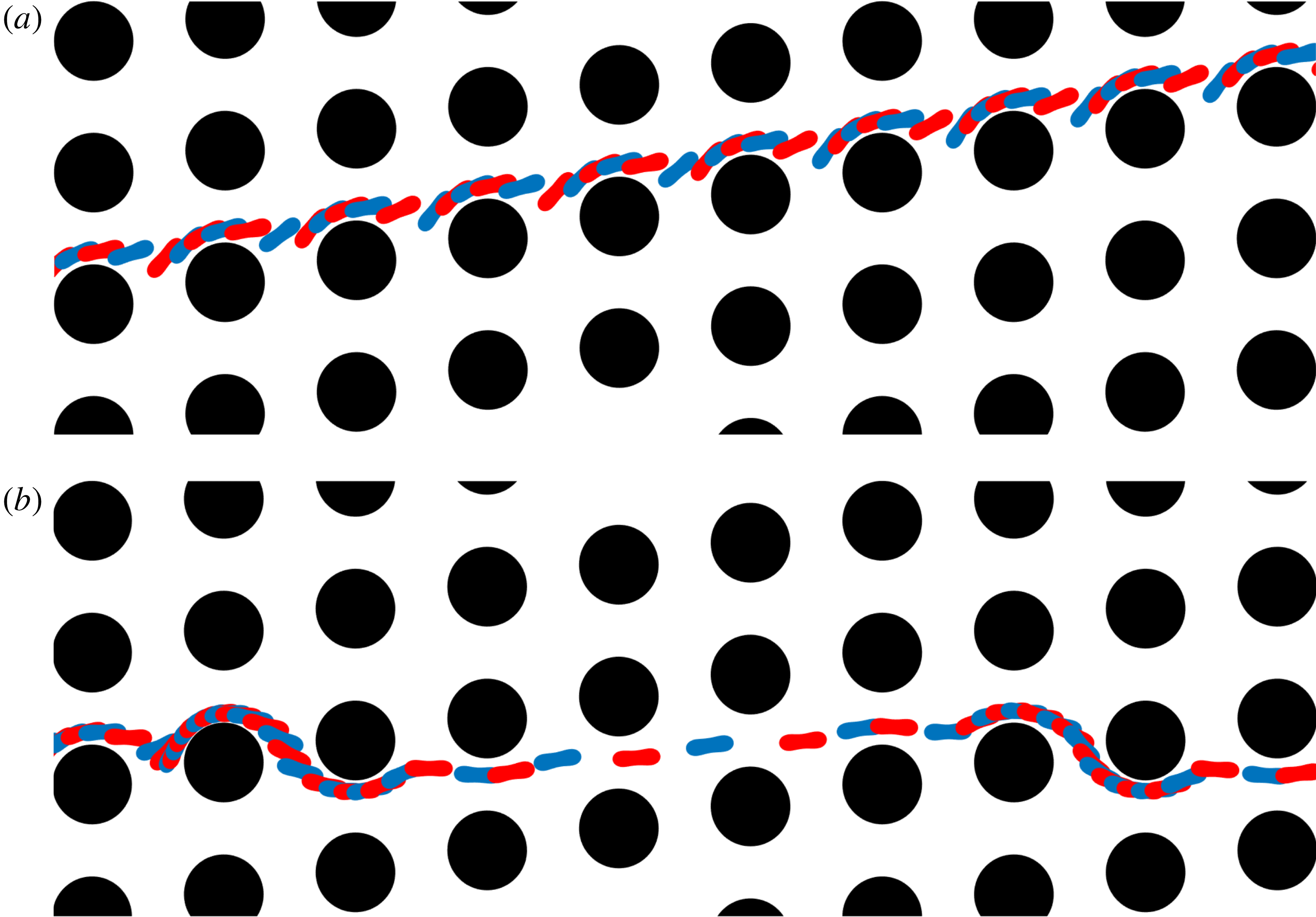
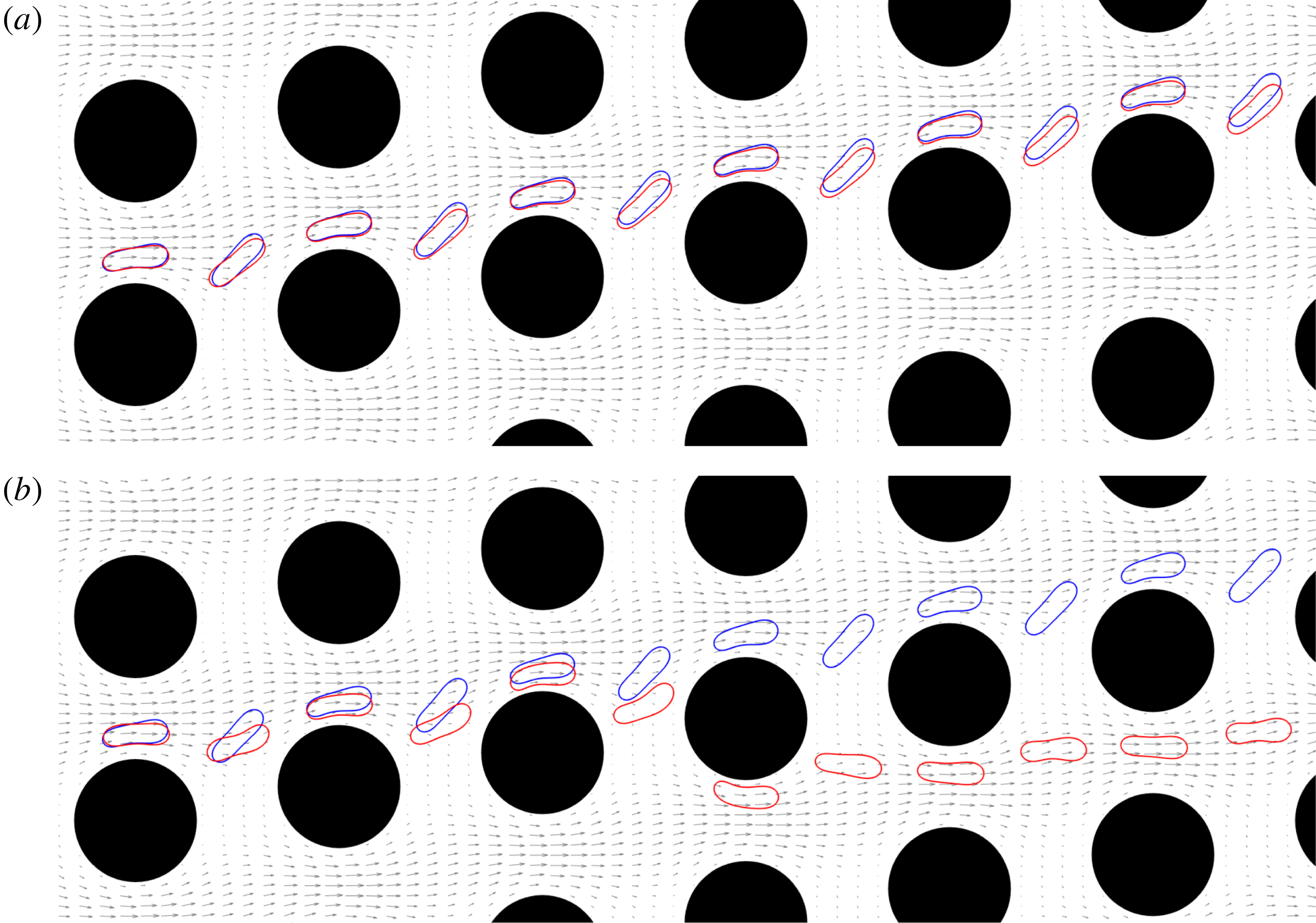
Transport modes of red blood cells (RBCs) flowing in a deterministic lateral displacement (DLD) device. The repeated blue–red RBC shapes indicate different time snapshots from the trajectory of a single cell. The DLD device consists of arrays of pillars (filled black circles). The flow is from left to right. Each pillar column is slightly shifted vertically with respect to the previous column. Separation of cells using DLD depends on their orientation, elasticity and viscosity. Here, the RBC in (a) has a lower viscosity than the one in (b). The less viscous RBC moves along the inclination of pillars while the more viscous one moves in the flow direction. The former transport mode is called ‘displacement’ and the latter is called ‘zig-zag’. After multiple interactions between the RBCs and the pillars, the displacing RBC shows more lateral displacement than the zig-zagging one. Thereby, they are laterally separated. Here, the tilt angle of the pillar rows is
 $0.17~\text{rad}$
.

Sorting biological cells by their mechanical properties (e.g. elasticity, cytoplasmic viscosity) is an important process in rapid medical diagnoses and tests using lab-on-a-chip technology. Therefore, microscale cell separation techniques have been of great interest. These techniques (see Bhagat et al. (Reference Bhagat, Bow, Houd, Tan, Han and Lim2010), Autebert et al. (Reference Autebert, Coudert, Bidard, Pierga, Descroix, Malaquin and Viovy2012) for an extensive review of them) take advantage of various cell fingerprints such as size, shape and deformability. For example, malaria-infected red blood cells and metastatic cancer cells can be differentiated based on their deformability as the malaria-infected cells are stiffer (Suresh et al. Reference Suresh, Spatz, Mills, Micoulet, Dao, Lim, Beil and Seufferlein2005) and the metastatic cancer cells are softer than their healthy counterparts (Guck et al. Reference Guck, Schinkinger, Lincoln, Wottawah, Ebert, Romeyke, Lenz, Erickson, Ananthakrishnan and Mitchell2005). The microscale cell separation techniques are divided into two categories: active and passive. The former uses an external force field, e.g. electrophoresis is an active method using an electric field to separate cells of different sizes and charges. Passive separation relies mainly on the device geometry and on hydrodynamic interactions between particles and the device. Thus, passive techniques are cheap and readily available. Deterministic lateral displacement (DLD) is a passive particle separation technique introduced by Huang et al. (Reference Huang, Cox, Austin and Sturm2004) to separate rigid particles from their dilute suspensions based on their sizes.
A DLD device consists of arrays of pillars (see figure 1). The pillar grid forms a lattice but the lattice vectors are not orthogonal. That is, the pillars are vertically aligned but their ‘horizontal’ or ‘diagonal’ alignment direction is at an angle with the
 $x$
-axis, which is also the flow direction axis. This arrangement determines a critical particle size (Davis et al.
Reference Davis, Inglis, Morton, Lawrence, Huang, Chou, Sturm and Austin2006). Particles larger than the critical size move along the direction defined by the pillars (see figure 1
a) while those smaller than the critical size move with the flow (see figure 1
b). The former transport mode is called ‘displacement’ and the latter is called ‘zig-zag’. After several particle–pillar interactions, the displacing particle is separated laterally from the zig-zagging one because the latter has almost zero net lateral displacement. Notice that figure 1 shows snapshots from simulations of cells; however, these trajectories are characteristic of the transport modes and the same for the rigid particles as well. Analytical DLD theory has been developed for dilute suspensions of rigid spherical particles under the assumption that the particle–pillar interactions dominate the particle–particle interactions in determining the particle trajectories. Critical particle sizes are computed and the devices are designed based on this assumption (Davis et al.
Reference Davis, Inglis, Morton, Lawrence, Huang, Chou, Sturm and Austin2006; Inglis et al.
Reference Inglis, Davis, Austin and Sturm2006; Davis Reference Davis2008). However, dilution of suspensions requires a pre-treatment of the sample, which is time-consuming and expensive and high volume fractions of suspensions are needed for high throughput. Therefore, the performance of DLD for dense suspensions is also of interest. Additionally, dynamics of non-spherical and deformable particles such as cells flowing in DLD devices needs to be investigated in order to design DLD devices for sorting those particles. So, although the DLD technique has been frequently used and is promising, several questions regarding its performance remain open. Given the wide spectrum of possible applications, here we focus on the sorting of human red blood cells.
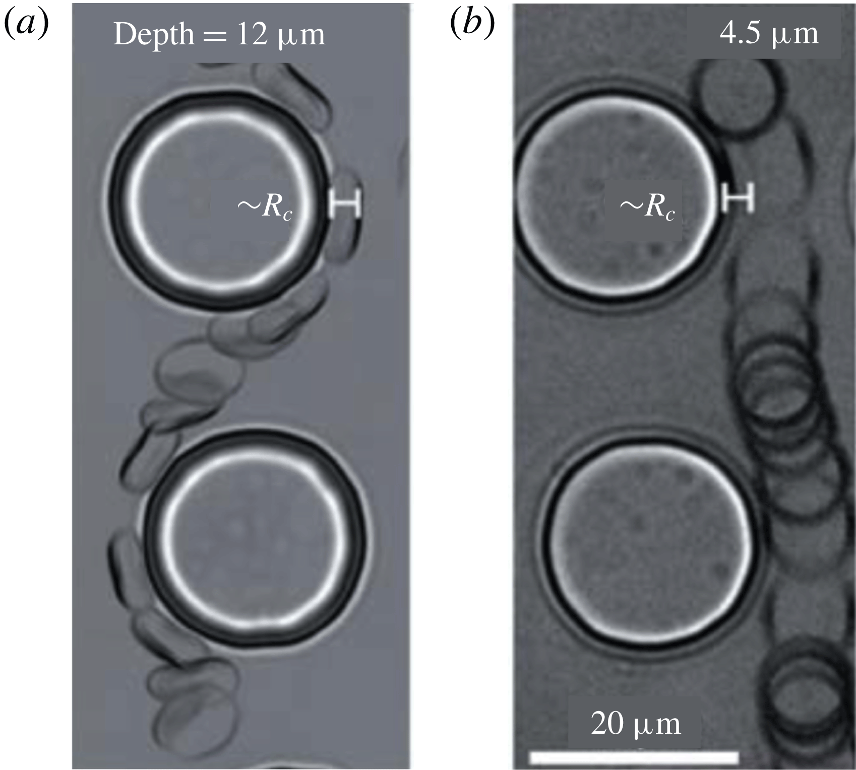
RBC orientations in a deep (a) and a shallow (b) DLD device (the images show the top view and are taken from Beech et al. (Reference Beech, Holm, Adolfsson and Tegenfeldt2012)). The heights of the pillars are
 $H=12~\unicode[STIX]{x03BC}\text{m}$
in the deep device and
 $H=4.5~\unicode[STIX]{x03BC}\text{m}$
in the shallow device. These are superimposed images of RBCs flowing in actual DLD devices. The fluid flows from top to bottom. In the deep device the RBC is orientated in a way that its thickness becomes its effective size. In the shallow device the confining walls in the out-of-plane direction push the RBC to move parallel to the walls. Therefore, what we see is a disc and the effective size is its diameter. The deep DLD devices are preferable to shallow ones in practice since they reduce the risk of clogging and provide higher throughput. We only consider deep devices in our study.

Human blood consists of plasma and mainly white and red blood cells and platelets. White blood cells (WBCs) are mostly spherical with a diameter in the range
 $5$
–
 $20~\unicode[STIX]{x03BC}\text{m}$
, red blood cells (RBCs) are biconcave with a diameter of
 $8~\unicode[STIX]{x03BC}\text{m}$
and a thickness of
 $3~\unicode[STIX]{x03BC}\text{m}$
and platelets are nearly rigid discoids (when they are not activated) with a diameter in the range
 $1$
–
 $3~\unicode[STIX]{x03BC}\text{m}$
(Popel & Johnson Reference Popel and Johnson2005). DLD has been used for fractionation of these components of human blood based on their sizes (Davis et al.
Reference Davis, Inglis, Morton, Lawrence, Huang, Chou, Sturm and Austin2006) and also used for separation of WBCs (Davis et al.
Reference Davis, Inglis, Morton, Lawrence, Huang, Chou, Sturm and Austin2006), RBCs (Zeming, Ranjan & Zhang Reference Zeming, Ranjan and Zhang2013), parasites (Holm et al.
Reference Holm, Beech, Barret and Tegenfeldt2011) and circulating tumour cells (Loutherback et al.
Reference Loutherback, D’Silva, Liu, Wu, Austin and Sturm2012; Karabacak et al.
Reference Karabacak, Spuhler, Fachin, Lim, Pai, Ozkumur, Martel, Kojic, Smith, Chen, Yang, Hwang, Morgan, Trautwein, Barber, Stott, Maheswaran, Kapur, Haber and Toner2014). Diseases such as sickle cell anaemia (Barabino Reference Barabino2010), diabetes (Buys et al.
Reference Buys, Van Rooy, Soma, Van Papendorp, Lipinski and Pretorius2013) and malaria are responsible for changes in RBC deformability by altering both the cytoplasmic viscosity and the membrane’s viscoelastic properties. Therefore, deformability-based sorting of RBCs could potentially identify and separate abnormal cells from blood. These considerations motivate our study of DLD devices. The parameters we used in this study are the membrane elasticity and cytoplasmic viscosity of RBCs, which determine their deformability.
A DLD device for RBC separation can be either shallow or deep (figure 2). A shallow device has short pillars with a height less than the RBC diameter (
 $H\approx 4{-}5~\unicode[STIX]{x03BC}\text{m}$
) while a deep one has tall pillars with a height much greater than the RBC diameter (
 $H\gg D_{RBC}$
). RBCs orient differently in these devices. A shallow device pushes cells parallel to the confining walls in the out-of-plane direction and results in an effective size (when they are not deformed) equal to the cell diameter. In a deep device they orient themselves in such a way that their effective size becomes their smallest size, i.e. their thickness. In shallow devices the separation of cells is similar to that of rigid spherical particles. While a suspension of stiff and soft cells flows through a shallow device, soft cells deform more than stiff cells and hence their effective size becomes smaller than that of the stiff cells. This results in zig-zagging soft cells and displacing stiff cells, and hence separation. However, throughput is limited in shallow devices. In contrast, deep devices allow more cells along the pillars and hence higher throughput. Cells can show richer dynamics in deep devices than shallow devices since deep devices do not confine cells in the out-of-plane direction as much as shallow ones do. Therefore, the separation in deep devices does not occur by the same means as in shallow devices. It depends on complex dynamics of cells, such as moving with a stationary angular orientation (i.e. tank-treading) or varying angular orientation (i.e. tumbling) (Henry et al.
Reference Henry, Holm, Zhang, Beech, Tegenfeldt, Fedosov and Gompper2016). RBCs show this complex dynamics in shear and Poiseuille flows depending on the cytoplasmic viscosity and membrane elasticity (Misbah Reference Misbah2006; Messlinger et al.
Reference Messlinger, Schmidt, Noguchi and Gompper2009; Podgorski et al.
Reference Podgorski, Callens, Minetti, Coupier, Dubois and Misbah2011; Misbah Reference Misbah2012; Fedosov, Peltomäki & Gompper Reference Fedosov, Peltomäki and Gompper2014). Cell dynamics in these fundamental flows has been studied and is well understood. However, the DLD flow is more complicated than these flows. How do such complex behaviours appear in deep DLD devices? How does sorting depend on them? How can we quantify them and explain sorting? These are the main questions we aim to address in this article.
1.1 Contributions
To the best of our knowledge, this is one of the first studies investigating the effects of the complex RBC dynamics in deep DLD devices. We show that deformability-based sorting of RBCs is possible. We list our contributions below.
(i) We investigate the cell dynamics in DLD flow, i.e. we study the inclination angle and lateral velocity of the cells in §§ 3.1 and 3.2.
(ii) We compare these cell-in-DLD dynamics with simple flows such as a free shear and confined Poiseuille flows in §§ 4.1 and 4.2.
(iii) In order to quantify migration, we compute a new quantity in § 4.3, which we call the ‘pseudo-lift’, that turns out to be an indicative measure of migration.
(iv) Lastly, we present phase diagrams for the transport modes in § 3.3 and investigate the separation in dense RBC suspensions in § 3.4 for different viscosity contrasts, capillary numbers and device configurations. The efficiency of DLD for dense suspensions in deep devices has not been studied experimentally or numerically. However, it is essential to investigate the dense suspension regime because the deep devices with dense suspensions provide higher throughput than the shallow devices with dilute suspensions.
Methodology. The main components of our approach is the mathematical model for the RBCs, the formulation and discretization and the DLD device set-up. Following Noguchi & Gompper (Reference Noguchi and Gompper2005) and Misbah (Reference Misbah2012), we model an RBC as an inextensible vesicle with a reduced area of 0.65 which resists deformation due to bending and tension. RBCs and vesicles share similar dynamical properties and the differences are minor in two dimensions. We assume the RBC membrane is impermeable to flow and locally inextensible. We assume that the fluids in the interior and exterior of the vesicle are Newtonian. Since the Reynolds number is
 $O(10^{-3})$
(see McGrath, Jimenez & Bridle (Reference McGrath, Jimenez and Bridle2014) for a summary of the experiments reported in the literature), we use a standard quasi-static Stokes approximation scheme to model the flow (Danker, Vlahovska & Misbah Reference Danker, Vlahovska and Misbah2009; Freund & Zhao Reference Freund and Zhao2010; Freund & Orescanin Reference Freund and Orescanin2011; Zhao & Shaqfeh Reference Zhao and Shaqfeh2011b
, Reference Zhao and Shaqfeh2013a
,Reference Zhao and Shaqfeh
b
). We formulate the problem as a set of integro-differential equations using a Nyström boundary integral method (Quaife & Biros Reference Quaife and Biros2014, Reference Quaife and Biros2015, Reference Quaife and Biros2016; Kabacaoğlu, Quaife & Biros Reference Kabacaoğlu, Quaife and Biros2017, Reference Kabacaoğlu, Quaife and Biros2018). Although many other methods can be used (Li, Vlahovska & Karniadakis Reference Li, Vlahovska and Karniadakis2013; Freund Reference Freund2014), boundary integral methods are known to work very well for Stokesian fluids with deformable interfaces (Pozrikidis Reference Pozrikidis2001, Reference Pozrikidis2003; Freund & Zhao Reference Freund and Zhao2010; Zhao & Shaqfeh Reference Zhao and Shaqfeh2013a
; Freund Reference Freund2014). Our numerical method for vesicle flows has been shown to be accurate and algorithmically optimal in the sense that it uses a linearly implicit time-stepping scheme to address stiffness due to bending, tension and near-field hydrodynamic interactions, it enforces inextensibility using Lagrange multipliers, it requires linear work (up to logarithmic factors) in terms of unknowns and it is spectrally accurate in space (and even in time (Quaife & Biros Reference Quaife and Biros2016)). For
 $m$
RBCs with
 $n$
points per RBC and
 $K$
time steps, our method costs
 $O(Kmn\log n)$
(Veerapaneni et al.
Reference Veerapaneni, Gueyffier, Zorin and Biros2009; Rahimian, Veerapaneni & Biros Reference Rahimian, Veerapaneni and Biros2010). Our DLD model has pillars with a circular cross-section only. Our two-dimensional (2-D) model can represent deep DLD devices not the shallow ones because RBCs with a reduced area of 0.65 in the 2-D model have the same orientation as RBCs in real deep devices (see figures 1 and 2). Additionally, our 2-D model does not include the wall effects and the cell–cell interactions in the out-of-plane direction which are negligible in deep devices but important in shallow ones. Unlike other numerical studies (discussed in § 1.3) we include multiple rows and columns of pillars in our simulation domain (this results in
 $O(100)$
pillars). We consider only one free parameter for the DLD device: the row-shift fraction
 $\unicode[STIX]{x1D716}$
(i.e. the angular orientation of the pillar orientation). We quantify an RBC’s elasticity and viscosity with two dimensionless numbers: the capillary number
 $C_{a}$
and viscosity contrast
 $\unicode[STIX]{x1D708}$
, respectively. First, we perform several simulations of RBCs with no viscosity contrast by changing the capillary number
 $C_{a}$
in a DLD with the row-shift fraction
 $\unicode[STIX]{x1D716}=0.1667$
. Second, in the same device we vary the viscosity contrast
 $\unicode[STIX]{x1D708}$
and fix the capillary number to
 $C_{a}=3.41$
, which corresponds to a value for the flow of a healthy RBC through DLD with an average velocity of
 $1~\text{mm}~\text{s}^{-1}$
. This flow speed is in the range (
 $1~\unicode[STIX]{x03BC}\text{m}~\text{s}^{-1}$
,
 $10~\text{mm}~\text{s}^{-1}$
) used in experiments on sorting RBCs depending on their deformability (McGrath et al.
Reference McGrath, Jimenez and Bridle2014). Additionally, it is not so high that cells do not deform significantly and hence we can observe the effects of viscosity contrast on cell dynamics. Last, we vary the viscosity contrast and capillary number for fixed row-shift fractions
 $\unicode[STIX]{x1D716}=0.1$
and
 $\unicode[STIX]{x1D716}=0.1667$
. Then we map out the parameter space for the transport modes as a function of
 $C_{a}$
,
 $\unicode[STIX]{x1D708}$
,
 $\unicode[STIX]{x1D716}$
. We also perform simulations of dense suspensions in DLD and quantify the efficiency of the technique for dense suspensions.
We summarize our findings as follows.
(i) Relation to cell migration. Cell migration is a phenomenon observed in a shear and confined Poiseuille flow. That is, cells having positive inclination with respect to the flow direction migrate towards low shear rate regions due to the parabolic velocity profile. In our numerical studies, we observe that more deformable cells have higher positive inclination angles with respect to the flow direction than the less deformable ones (see § 4.2). Since the velocity profile near the pillars is parabolic, the more deformable cells migrate further away from the pillars than the less deformable ones. Thus, the more deformable cells displace while the less deformable ones zig-zag.
(ii) Effects of complex geometry. Although we have discovered that cell dynamics in DLD gaps is similar to that in confined Poiseuille flows (see § 4.2), the dynamics in the whole device is more complicated than the channel flow because a cell periodically moves from a confined gap to a less confined region between gaps. (By ‘DLD’ gap, we refer to the flow space between two vertically aligned pillars.) So it is not possible to estimate the cell dynamics in DLD from a simpler flow such as a channel flow.
(iii) Quantification of migration. We have computed the cell vertical migration velocity in DLD and demonstrated that it correlates well with the inclination angle (see § 4.2).
(iv) Pseudo-lift. By computing the so-called pseudo-lift (a measure of the alignment of local forces to the migration direction) acting for several cells, we have found
 $5\times$
stronger pseudo-lift on cells with high inclination angles compared to cells with smaller inclination angles which are under either a negative or a weak pseudo-lift (see § 4.3).
(v) Dense suspensions. Finally, when we assessed the DLD efficiency for dense RBC suspensions, we have observed that most cells zig-zag in dense suspensions no matter what their capillary numbers and viscosity contrasts are. So it is difficult to separate small rigid particles or stiff cells from dense suspensions because these would zig-zag, too. This result agrees with the numerical (Vernekar & Krüger Reference Vernekar and Krüger2015) and experimental (Inglis, Lord & Nordon Reference Inglis, Lord and Nordon2011) studies which use shallow devices (see § 3.4).

1.2 Limitations
Our modelling approaches have several limitations. First, our simulations are in two dimensions. We have opted to use two-dimensional simulations because three-dimensional simulations of a DLD device including multiple pillars can be quite expensive for this purpose (Rossinelli et al. Reference Rossinelli, Tang, Lykov, Alexeev, Bernaschi, Hadjidoukas, Bisson, Joubert, Conti, Karniadakis, Fatica, Pivkin and Koumoutsakas2015). Two-dimensional studies have been proved to be predictive and match actual experiments in many regimes (e.g. motion of RBCs in microchannels (Kaoui et al. Reference Kaoui, Tahiri, Biben, Ez-Zahraouy, Benyoussef, Biros and Misbah2011; Fedosov et al. Reference Fedosov, Peltomäki and Gompper2014), margination of white blood cells in blood flow (Freund Reference Freund2007; Zhao & Shaqfeh Reference Zhao and Shaqfeh2011a ; Müller, Fedosov & Gompper Reference Müller, Fedosov and Gompper2014) and sorting of rigid particles using deterministic lateral displacement technique (Zhang et al. Reference Zhang, Henry, Gompper and Fedosov2015)). Second, our numerical scheme is valid only for Newtonian flows with no inertia (zero Reynolds number) and does not permit viscoelastic fluids in the interior and the exterior of the RBCs. Finally, our RBC model does not have a spectrin network.
Despite the limitations of our model, it reproduces actual experimental results without any tuning parameters. For example, it reproduces the phase diagram for size-based sorting of rigid spherical particles. Our model allows us to explore the underlying DLD physics and explore the parameter space. However, our simulations do not shed light on several other factors affecting cell sorting. One of them is the effects of changes in the resting size and shape of an RBC. When an RBC becomes diseased, not only its elasticity and viscosity change but also its resting size. The other one is the effect (on cell sorting) of the lateral confinement in the DLD gaps. In our study, the confinement in the gaps does not allow a cell to tumble and leads it to move always with a positive inclination angle. In the case of a weaker confinement, the cell can tumble for high viscosity contrasts (i.e. for less deformable cases). We expect tumbling to increase the cell’s effective size in those cases and hence result in displacing of cells. For example, Zeming et al. (Reference Zeming, Ranjan and Zhang2013) and Ranjan et al. (Reference Ranjan, Zeming, Jureen, Fisher and Zhang2014) observed that pillars with protrusions cause cells to tumble and tumbling cells start displacing for the same reason. Finally, we do not consider the effects of adhesion on cell sorting, which could be important for dense RBC suspensions. Blood suspensions are usually diluted in real applications (McGrath et al. Reference McGrath, Jimenez and Bridle2014). In dilute suspensions the distance between the cell and the pillars is much greater than the adhesion length scale. Hence, we do not expect any adhesion effects on our results for a single cell flowing through a DLD device.
1.3 Related work
The study in Henry et al. (Reference Henry, Holm, Zhang, Beech, Tegenfeldt, Fedosov and Gompper2016) is very similar to ours and the findings are consistent. They study both deep and shallow devices by combining simulations (3-D smoothed dissipative particle dynamics) and experiments. They only consider three viscosity contrast values (0.25, 1, 5), whereas we study a much wider range of viscosity contrasts (up to 100). Also, we vary the capillary number (they do not). Going beyond the work in Henry et al. (Reference Henry, Holm, Zhang, Beech, Tegenfeldt, Fedosov and Gompper2016), we conduct a systematic study and map out the parameter space for the transport modes of cells. We investigate the cell dynamics in DLD in detail and compare those dynamics with simpler flows such as confined Poiseuille flow. We claim that cell migration is responsible for cell separation in DLD and quantify migration with migration velocity and pseudo-lift. Henry et al. (Reference Henry, Holm, Zhang, Beech, Tegenfeldt, Fedosov and Gompper2016) shows our 2-D simulations can capture the actual experiments and support our findings and rationale.
In addition to Henry et al. (Reference Henry, Holm, Zhang, Beech, Tegenfeldt, Fedosov and Gompper2016) mentioned above, there have been a few numerical studies investigating the separation of deformable particles using DLD:
(i) Quek, Le & Chiam (Reference Quek, Le and Chiam2011) and Ye et al. (Reference Ye, Shao, Yu and Yu2014) performed two-dimensional simulations of spherical deformable particles with no viscosity contrast in order to explain the effects of particle deformability on the separation,
(ii) Krüger, Holmes & Coveney (Reference Krüger, Holmes and Coveney2014) systematically investigated the effects of the capillary number
$C_{a}$
on the separation of RBCs with a constant viscosity contrast of
$\unicode[STIX]{x1D708}=5$
in shallow devices using three-dimensional simulations,(iii) Zhang et al. (Reference Zhang, Henry, Gompper and Fedosov2015) studied circular, square, diamond and triangular pillar shapes for the separation of rigid particles and RBCs using two-dimensional simulations.


Overall, none of these studies have systematically investigated the separation of RBCs as a function of the capillary number and viscosity contrast in deep devices.
Regarding numerical methods, all the studies above used either the immersed boundary method (Quek et al. Reference Quek, Le and Chiam2011; Krüger et al. Reference Krüger, Holmes and Coveney2014; Vernekar & Krüger Reference Vernekar and Krüger2015), lattice-Boltzmann method (Krüger et al. Reference Krüger, Holmes and Coveney2014; Vernekar & Krüger Reference Vernekar and Krüger2015), fictitious domain method (Ye et al. Reference Ye, Shao, Yu and Yu2014) or dissipative particle dynamics (Zhang et al. Reference Zhang, Henry, Gompper and Fedosov2015; Henry et al. Reference Henry, Holm, Zhang, Beech, Tegenfeldt, Fedosov and Gompper2016). Here, we use our in-house algorithms based on the boundary integral equation formulation for Stokesian particulate flows (Kabacaoğlu et al. Reference Kabacaoğlu, Quaife and Biros2018). We refer the reader to Veerapaneni et al. (Reference Veerapaneni, Gueyffier, Zorin and Biros2009), Rahimian et al. (Reference Rahimian, Veerapaneni and Biros2010), Quaife & Biros (Reference Quaife and Biros2014, Reference Quaife and Biros2015, Reference Quaife and Biros2016) for the details of our scheme and the review of the numerical methods for Stokesian particulate flows. Additionally, most numerical studies of DLD mentioned in the previous paragraph reduced the simulation domain to a single pillar and used periodic boundary conditions. Since actual DLD devices have walls that result in zero net lateral flow, an artificial force in the lateral direction needs to be introduced to mimic the wall effects in the periodic models (D’Avino Reference D’Avino2013). Our model contains multiple pillars in the lateral and flow directions, and also the top and bottom walls. Therefore, we do not need to add any force mimicking the wall effects. The only parameters in our scheme are the physical parameters (device geometry, number of cells, viscosity contrast and capillary number) as well as the spatial discretization size. We use an adaptive, semi-implicit time-stepping scheme. No other (non-physical) parameters are necessary. We only have five free parameters in our model (other than the shape of the device): the time-step error tolerance, the points per cell, the discretization size of the rigid walls, the viscosity contrast and the capillary number. We have also performed a convergence study to verify our method in the DLD setting in appendix C.
There is only one numerical study (Vernekar & Krüger Reference Vernekar and Krüger2015) where simulations of dense RBC suspensions with different volume fractions were performed in shallow devices. The authors found that the displacement mode breaks down as the volume fraction increases and most of the RBCs zig-zag independently of the capillary number. We also studied this by performing simulations of dense RBC suspensions with two different capillary numbers and volume fractions in deep devices. We reached the same conclusions. In addition, we considered dense RBC suspensions with different viscosity contrasts. Our results show that, again, the displacement mode breaks down.
There are efforts to develop novel pillar shapes in order to improve the DLD performance. Zeming et al. (Reference Zeming, Ranjan and Zhang2013) presented I-shaped pillars for RBC separations and showed that the I-shape increases the RBCs’ effective sizes by inducing rotational motions. Ranjan et al. (Reference Ranjan, Zeming, Jureen, Fisher and Zhang2014) conducted experiments with various pillar shapes to investigate efficient separation of spherical and non-spherical bio-particles. They considered pillars with protrusions and grooves to induce particle rotation and maintain the rotational movement in the flow direction. We observed that there is a need for novel shapes to prevent breakdown of the displacement mode for the dense RBC suspensions, so that small particles (which would zig-zag) can effectively be separated from dense suspensions. However, this is beyond the scope of the current study.
1.4 Outline of the paper
In § 2.1 we briefly summarize the governing equations for the RBC flows. We explain the DLD theory in detail and our DLD model in § 2.2. After validating our model by comparing our numerical results for the size-based separation of rigid particles with the actual experiments (Davis Reference Davis2008) in § 2.4, we present our results in § 3. We show snapshots from the simulations in §§ 3.1 (for different capillary numbers) and 3.2 (for different viscosity contrasts). We present the phase diagrams of the transport modes as a function of
 $C_{a}$
,
 $\unicode[STIX]{x1D708}$
and
 $\unicode[STIX]{x1D716}$
in § 3.3. In § 3.4 we demonstrate the failure rates of the transport modes in dense suspensions of RBCs. Then, in § 4 we quantify the cell dynamics in DLD and compare it with that in shear and confined Poiseuille flows. Finally, we summarize our results in § 5. In appendix A we present the detailed integral equation formulation for the Stokesian particulate flows. Then we show that our DLD model is insensitive to the number of pillars in the domain when capturing the particle trajectories in appendix B and we show convergence studies for verification of our solver in appendix C.
1.5 Notation
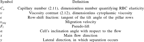
We summarize the main notation used in this paper in table 1.
List of frequently used notation.

2 Numerical model and geometry
We present the mathematical model for the flow of red blood cells in § 2.1 and our DLD model in § 2.2. We verify and validate our DLD model by comparing our numerical results for the separation of rigid spherical particles with the experimental data available in the literature in §§ 2.3 and 2.4. Finally, in § 2.5 we describe the dimensionless parameters for which we will investigate effects on the RBC separation.
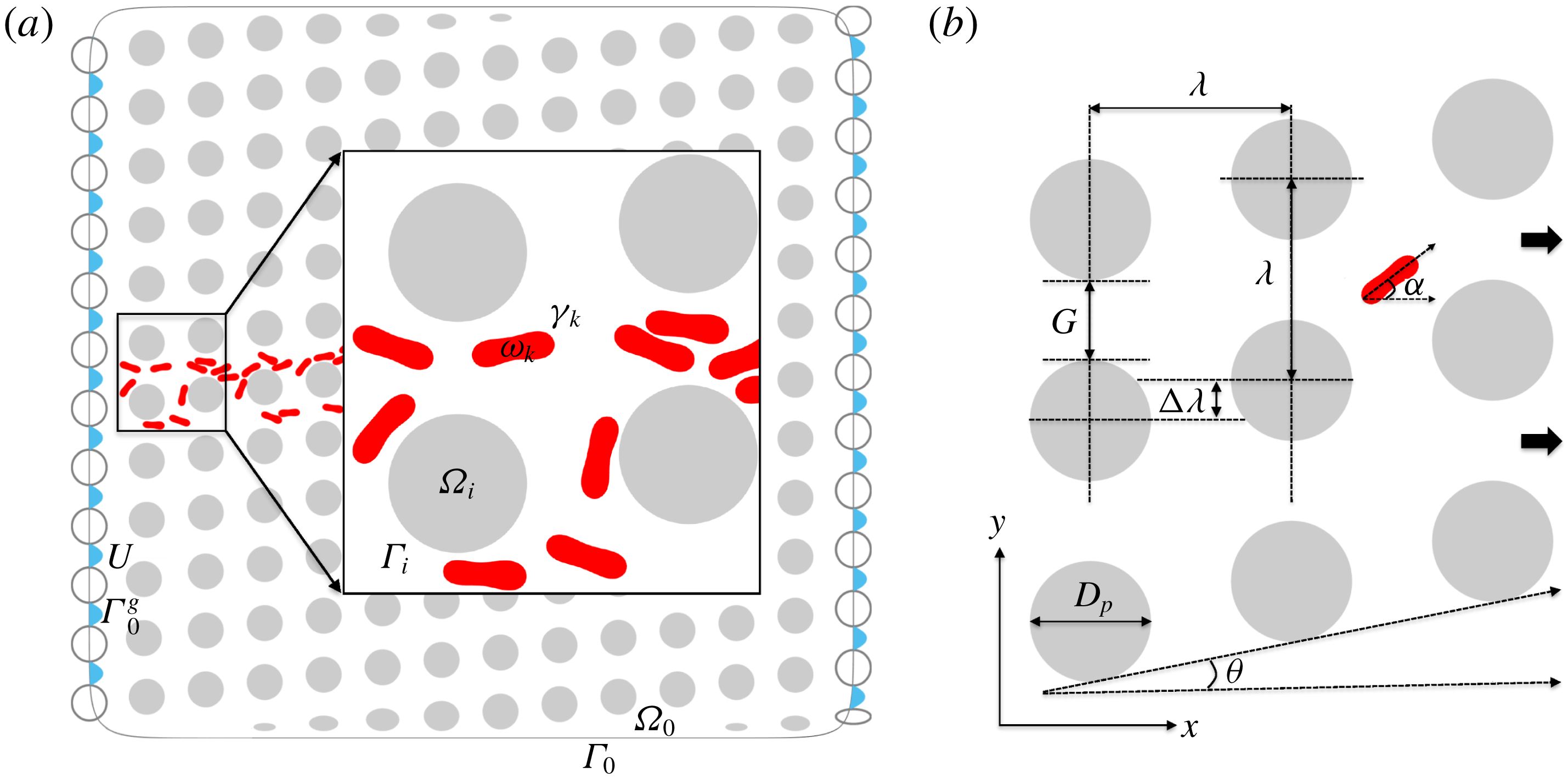
We illustrate the domain of a cell suspension in a DLD device in (a). We model RBCs as inextensible vesicles with a reduced area of 0.65. The interior and boundary of the
 $i$
th pillar are denoted by
 $\unicode[STIX]{x1D6FA}_{i}$
and
 $\unicode[STIX]{x1D6E4}_{i}$
(
 $\unicode[STIX]{x1D6FA}_{0}$
and
 $\unicode[STIX]{x1D6E4}_{0}$
are the ones of the exterior wall). Additionally,
 $\unicode[STIX]{x1D714}_{k}$
and
 $\unicode[STIX]{x1D6FE}_{k}$
stand for the interior and boundary of the
 $k$
th cell. The empty circles are the pillars in the left and the right imaginary columns. The walls pass through these pillars’ centres. The blue arrows show the parabolic velocity
 $\boldsymbol{U}$
imposed as a boundary condition in the gaps
 $\unicode[STIX]{x1D6E4}_{0}^{g}$
between the imaginary pillars. In (b) we show the DLD parameters where
 $x$
is the flow direction. The geometry is uniquely defined by the pillar diameter
 $D_{p}$
, the centre-to-centre distance
 $\unicode[STIX]{x1D706}$
and the row shift
 $\unicode[STIX]{x0394}\unicode[STIX]{x1D706}$
. Using these parameters we can determine the gap size
 $G$
, the row-shift fraction
 $\unicode[STIX]{x1D716}=\unicode[STIX]{x0394}\unicode[STIX]{x1D706}/\unicode[STIX]{x1D706}$
and the tilt angle of the pillars (the angle between the flow direction and the alignment direction of the pillars)
 $\unicode[STIX]{x1D703}=\tan ^{-1}(\unicode[STIX]{x1D716})$
. The red cell in (b) has a positive inclination angle
 $\unicode[STIX]{x1D6FC}$
with respect to the flow direction, which is defined in § 2.1.

2.1 Governing equations
We assume that the flow is two-dimensional and there are no external body forces such as gravity. Both the RBC’s interior fluid and the exterior fluid (plasma) are Newtonian. We assume a Stokesian fluid. See figure 3(a) for the geometry. Let the boundary of each pillar be denoted by
 $\unicode[STIX]{x1D6E4}_{i}$
. The pillars are bounded by an exterior wall
 $\unicode[STIX]{x1D6E4}_{0}$
which is a mollification of a rectangle. The areas enclosed by the exterior wall and the
 $i$
th pillar are denoted with
 $\unicode[STIX]{x1D6FA}_{0}$
and
 $\unicode[STIX]{x1D6FA}_{i}$
, respectively. Therefore, the suspension resides in the domain
 $$\begin{eqnarray}\displaystyle \unicode[STIX]{x1D6FA}=\unicode[STIX]{x1D6FA}_{0}\bigg\backslash\left(\mathop{\bigcup }_{i}\unicode[STIX]{x1D6FA}_{i}\right), & & \displaystyle\end{eqnarray}$$
and its boundary is
 $\unicode[STIX]{x1D6E4}=\unicode[STIX]{x1D6E4}_{0}\cup (\bigcup _{i}\unicode[STIX]{x1D6E4}_{i})$
.
The reduced area,
 $4\unicode[STIX]{x03C0}A/P^{2}$
, is the ratio between the area of a cell
 $A$
and the area of a circle having the same perimeter
 $P$
. We model RBCs as inextensible capsules with bending (vesicles) and with a reduced area of 0.65. For this reduced area the vesicles exhibit a biconcave shape as RBCs. A cell’s inclination angle
 $\unicode[STIX]{x1D6FC}$
(see also figure 3
b) is the angle between the flow direction and the principal axis corresponding to the smallest principal moment of inertia (Rahimian et al.
Reference Rahimian, Veerapaneni and Biros2010). The moment of inertia tensor is
 $$\begin{eqnarray}\displaystyle J=\frac{1}{4}\int _{\unicode[STIX]{x1D6FE}_{k}}\boldsymbol{r}\boldsymbol{\cdot }\boldsymbol{n}(|\boldsymbol{r}|^{2}\unicode[STIX]{x1D644}-\boldsymbol{r}\otimes \boldsymbol{r})\,\text{d}\unicode[STIX]{x1D6FE}_{k}. & & \displaystyle\end{eqnarray}$$
Here,
 $\boldsymbol{r}=\boldsymbol{x}-\boldsymbol{c}$
and
 $\boldsymbol{c}$
is the centre of the cell.
 $\unicode[STIX]{x1D6FE}_{k}$
and
 $\unicode[STIX]{x1D714}_{k}$
stand for the boundary and interior of the
 $k$
th cell, respectively. Let
 $\unicode[STIX]{x1D6FE}=\bigcup _{k}\unicode[STIX]{x1D6FE}_{k}$
and
 $\unicode[STIX]{x1D714}=\bigcup _{k}\unicode[STIX]{x1D714}_{k}$
, then the equations describing velocity field at an instance are given by
 $$\begin{eqnarray}\displaystyle -\unicode[STIX]{x1D702}\unicode[STIX]{x0394}\boldsymbol{u}(\boldsymbol{x})+\unicode[STIX]{x1D735}p(\boldsymbol{x})=0,\quad \text{and}\quad \text{div}(\boldsymbol{u}(\boldsymbol{x}))=0,\quad \boldsymbol{x}\in \unicode[STIX]{x1D6FA}\setminus \unicode[STIX]{x1D6FE}. & & \displaystyle\end{eqnarray}$$
Here,
 $\unicode[STIX]{x1D702}$
is the viscosity (
 $\unicode[STIX]{x1D702}_{in}$
for the interior and
 $\unicode[STIX]{x1D702}_{out}$
for the exterior fluid),
 $\boldsymbol{u}$
is the velocity and
 $p$
is the pressure. We impose the velocity on the external wall and pillars as a Dirichlet boundary condition (we explain the boundary conditions in detail in § 2.2)
 $$\begin{eqnarray}\displaystyle \boldsymbol{u}(\boldsymbol{x},t)=\boldsymbol{U}(\boldsymbol{x},t),\quad \boldsymbol{x}\in \unicode[STIX]{x1D6E4}. & & \displaystyle\end{eqnarray}$$
Conservation of mass and the no-slip boundary condition require velocity continuity on the interface of cells, i.e.
 $$\begin{eqnarray}\displaystyle \boldsymbol{u}(\boldsymbol{x},t)=\frac{\text{d}\boldsymbol{x}}{\text{d}t}(t),\quad \boldsymbol{x}\in \unicode[STIX]{x1D6FE}. & & \displaystyle\end{eqnarray}$$
RBCs are known to be inextensible, i.e. they conserve their area and arc-length in two dimensions. Inextensibility means that
 $$\begin{eqnarray}\displaystyle \boldsymbol{x}_{s}\boldsymbol{\cdot }\boldsymbol{u}_{s}=0,\quad \boldsymbol{x}\in \unicode[STIX]{x1D6FE}, & & \displaystyle\end{eqnarray}$$
where the subscript ‘
 $s$
’ stands for differentiation with respect to the arc-length on the boundaries of cells. The last governing equation comes from the momentum balance on the interface of the cells. Since the cells resist bending and tension, the interface applies an elastic force as a result of deformation due to them. The momentum balance enforces the jump in the surface traction to be equal to the net elastic force applied by the interface,
 $$\begin{eqnarray}\displaystyle \unicode[STIX]{x27E6}\unicode[STIX]{x1D64F}\boldsymbol{n}(\boldsymbol{x})\unicode[STIX]{x27E7}=-\unicode[STIX]{x1D705}_{b}\boldsymbol{x}_{ssss}+(\unicode[STIX]{x1D70E}(\boldsymbol{x},t)\boldsymbol{x}_{s})_{s},\quad \boldsymbol{x}\in \unicode[STIX]{x1D6FE}, & & \displaystyle\end{eqnarray}$$
where
 $\unicode[STIX]{x1D64F}=-p\unicode[STIX]{x1D644}+\unicode[STIX]{x1D702}(\unicode[STIX]{x1D735}\boldsymbol{u}+\unicode[STIX]{x1D735}\boldsymbol{u}^{\text{T}})$
is the Cauchy stress tensor,
 $\boldsymbol{n}$
is the outward normal vector on
 $\unicode[STIX]{x1D6FE}$
,
 $\unicode[STIX]{x27E6}\cdot \unicode[STIX]{x27E7}$
is the jump across the interface. The right-hand side is the net force applied by the interface onto the fluid. The first term on the right-hand side is the force due to bending stiffness
 $\unicode[STIX]{x1D705}_{b}$
and the second term is the force due to tension
 $\unicode[STIX]{x1D70E}$
, which acts as a Lagrange multiplier enforcing the inextensibility (Veerapaneni et al.
Reference Veerapaneni, Gueyffier, Zorin and Biros2009). Finally, the position of the boundaries of
 $M$
cells evolves as
 $$\begin{eqnarray}\displaystyle \frac{\text{d}\boldsymbol{x}_{i}}{\text{d}t}=\boldsymbol{u}_{\infty }(\boldsymbol{x}_{i})+\mathop{\sum }_{j=1}^{M}\boldsymbol{u}(\boldsymbol{x}_{j}),\quad i=1,\ldots ,M, & & \displaystyle\end{eqnarray}$$
where
 $\boldsymbol{u}_{\infty }(\boldsymbol{x}_{i})$
is the background velocity and
 $\boldsymbol{u}(\boldsymbol{x}_{j})$
is the velocity due to the
 $j$
th cell acting on the
 $i$
th cell.
The complete set of nonlinear equations (2.3)–(2.8) governs the evolution of the cell interfaces. In line with our previous work (Veerapaneni et al. Reference Veerapaneni, Gueyffier, Zorin and Biros2009; Rahimian et al. Reference Rahimian, Veerapaneni and Biros2010; Quaife & Biros Reference Quaife and Biros2014, Reference Quaife and Biros2015, Reference Quaife and Biros2016; Kabacaoğlu et al. Reference Kabacaoğlu, Quaife and Biros2018), we use an integral equation method to obtain the positions of the cell boundaries (see Kabacaoğlu et al. (Reference Kabacaoğlu, Quaife and Biros2018) for the details of the numerical scheme). The method can naturally handle the moving geometry, achieves high-order accuracy with a low computational cost and can handle the viscosity contrast between the interior and exterior fluid. For completeness, we present the integral equation formulation in appendix A.
2.2 DLD model
A DLD device of circular pillars can be uniquely determined by three parameters: the diameter of a pillar
 $D_{p}$
, the centre-to-centre distance between two neighbouring pillars
 $\unicode[STIX]{x1D706}$
and the row shift
 $\unicode[STIX]{x0394}\unicode[STIX]{x1D706}$
. See figure 3(b) for the DLD geometry.
Geometry. Our DLD device consists of circular pillars all of which have the same diameter
 $D_{p}=15~\unicode[STIX]{x03BC}\text{m}$
. The fluid flows in the
 $x$
direction. The centre-to-centre distance between neighbouring pillars is
 $\unicode[STIX]{x1D706}=25~\unicode[STIX]{x03BC}\text{m}$
and the same in both directions. This results in a gap size of
 $G=\unicode[STIX]{x1D706}-D_{p}=10~\unicode[STIX]{x03BC}\text{m}$
. Pillars centred at the same
 $x$
coordinate form a ‘column’. Each pillar in a neighbouring column is shifted by
 $\unicode[STIX]{x0394}\unicode[STIX]{x1D706}$
in the
 $y$
direction with respect to the previous one, which defines the row-shift fraction
 $\unicode[STIX]{x1D716}=\unicode[STIX]{x0394}\unicode[STIX]{x1D706}/\unicode[STIX]{x1D706}$
. Thus, the ‘rows’ are tilted with an angle
 $\unicode[STIX]{x1D703}=\tan ^{-1}(\unicode[STIX]{x1D716})$
. We define ‘lane’ to be a path between two diagonally parallel rows.
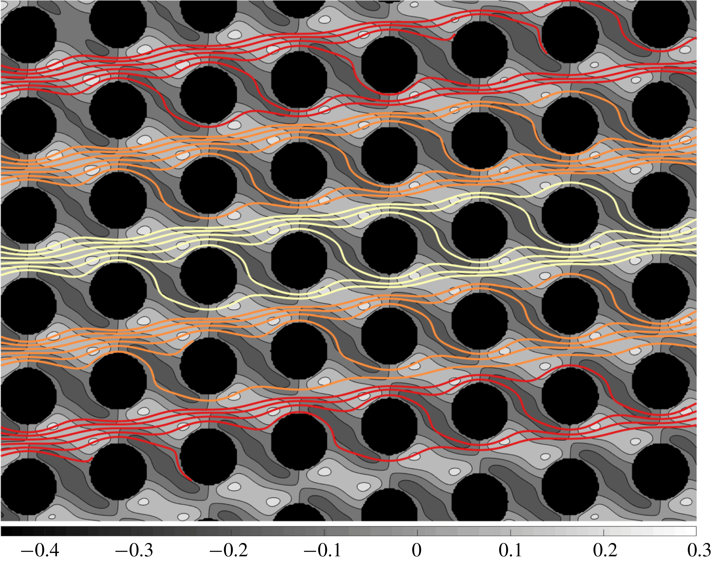
Velocity in the vertical direction (represented by grey-scale contours) with streamlines in the absence of particles superimposed. The row-shift fraction is
 $\unicode[STIX]{x1D716}=0.1667$
, which corresponds to the period
 $n_{p}=6$
. The flow is from left to right. See figure 5 for the velocity magnitude in the whole device and the velocity field in a gap. Each streamline interacts with a pillar, then swaps a lane. The DLD theory assumes that rigid particles do not distort the streamlines significantly. Depending on their size, they either follow these streamlines in zig-zag mode or cross the streamlines and stay in the same lane in displacement mode.

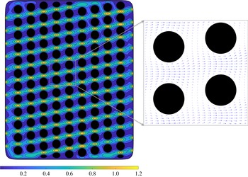
Velocity magnitude (on the left) and velocity in a gap (on the right) in our DLD model for
 $\unicode[STIX]{x1D716}=0.1667$
, i.e.
 $n_{p}=6$
. Our DLD model consists of 12 rows and
 $\lceil 1.5n_{p}\rceil$
columns of pillars (i.e. 9 columns here). We draw the side walls such that they pass through the centres of the shifted imaginary columns (not shown). Then we impose a parabolic velocity profile (2.9) on the boundaries which correspond to the gaps between the imaginary pillars as a boundary condition. We replaced the circular pillars crossing the top and the bottom walls with the elliptical ones. That leads to a homogeneous velocity in the device. See figure 4 for the velocity in the
 $y$
direction and the streamlines for this DLD configuration.

DLD theory for rigid spherical particles. The row-shift fraction
 $\unicode[STIX]{x1D716}$
sets what is referred to as the period
 $p$
of the device. ‘Period’ sets a length scale in which the column arrangement is exactly repeated. Therefore, we can divide the unperturbed flow in a gap (i.e. in the absence of any particles) into
 $n_{p}$
flow streams of equal mass flux. If we assume that the unperturbed flow does not change significantly when particles flow, the width of the stream adjacent to a pillar becomes the critical particle size (Davis et al.
Reference Davis, Inglis, Morton, Lawrence, Huang, Chou, Sturm and Austin2006). Particles small enough to fit into one of the streams stay in their streams by zig-zagging, whereas the larger ones cannot. As the tilt angle
 $\unicode[STIX]{x1D703}$
reduces (i.e. the row-shift fraction
 $\unicode[STIX]{x1D716}$
reduces or the period
 $n_{p}$
increases), the stream width decreases and hence the critical particle size decreases. This theory is in good agreement with experiments with spherical rigid particles (Davis et al.
Reference Davis, Inglis, Morton, Lawrence, Huang, Chou, Sturm and Austin2006; Davis Reference Davis2008).
Simulation domain. DLD devices usually consist of
 $O(10)$
rows and
 $O(100)$
columns, which results in
 $O(1000)$
pillars in a device. Performing simulations of cell separation in a whole DLD device is computationally expensive (Rossinelli et al.
Reference Rossinelli, Tang, Lykov, Alexeev, Bernaschi, Hadjidoukas, Bisson, Joubert, Conti, Karniadakis, Fatica, Pivkin and Koumoutsakas2015). This renders its systematic analysis infeasible even in two dimensions. In order to evade the computational cost, the numerical studies conducted so far in this area reduced the simulation domain to a single pillar by assuming periodicity (Quek et al.
Reference Quek, Le and Chiam2011; Krüger et al.
Reference Krüger, Holmes and Coveney2014; Ye et al.
Reference Ye, Shao, Yu and Yu2014; Vernekar & Krüger Reference Vernekar and Krüger2015; Zhang et al.
Reference Zhang, Henry, Gompper and Fedosov2015). However, one pillar with periodic conditions requires imposing an artificial lateral force to enforce zero net lateral flow since in real DLD devices the lateral flow is restricted by the walls.
Due to the high computational costs, most of our numerical experiments are conducted using only one period, i.e. at least
 $\lceil 1/\unicode[STIX]{x1D716}\rceil$
pillars in the flow direction instead of using just one pillar. We confine the pillar lattice with an exterior wall to enforce zero net lateral flow. This raises the questions as to whether the wall effects introduce large errors. We numerically determined that the errors are negligible if we use 12 pillars in the
 $y$
direction (i.e. 12 rows) and
 $\lceil 1.5(1/\unicode[STIX]{x1D716})\rceil$
pillars in the
 $x$
direction (i.e.
 $\lceil 1.5(1/\unicode[STIX]{x1D716})\rceil$
columns) (see figures 3
a and 5 as an example). We present the details of this analysis in appendix B. The initial locations of the cells are in the middle lane. Since the pillars are shifted laterally, we end up with pillars crossing the exterior wall at the top and the bottom. We found out that if we just remove those pillars, the empty spaces result in less hydraulic resistance and hence induce a lateral pressure gradient. This breaks the homogeneity of the flow and introduces significant errors in the cell trajectories (Kulrattanarak et al.
Reference Kulrattanarak, van der Sman, Schröen and Boom2011; Vernekar et al.
Reference Vernekar, Krüger, Loutherback, Morton and Inglis2017). Therefore, we decided to replace the circular pillars crossing the walls with elliptical pillars in such a way that they maintain the same vertical spacing with the neighbouring pillars. Those non-circular pillars near the top and bottom walls provided a homogeneous flow in the middle region in our model (see figure 5 for our DLD model and the unperturbed velocity for
 $n_{p}=6$
).
Henry et al. (Reference Henry, Holm, Zhang, Beech, Tegenfeldt, Fedosov and Gompper2016) showed that RBCs might have additional zig-zag modes unlike rigid particles, such as zig-zagging within a period or zig-zagging that requires more than a period to take place. In order to capture those zig-zagging modes, we perform simulations of a cell by initializing it at several lateral positions. This is equivalent to simulating the cell for more than one period because in each simulation the cell confronts the first pillar at a different lateral position. We label the cell as zig-zagging if it zig-zags in any of these simulations and as displacing if it displaces in all of the simulations.
Boundary conditions. We want to reflect the periodicity of the DLD device in our model by imposing the velocity as a boundary condition at the intake and the outtake. For this purpose, we place the side walls as if they pass through the imaginary columns of the pillars shifted down on the left and up on the right by
 $\unicode[STIX]{x0394}\unicode[STIX]{x1D706}$
(the empty circles in figure 3
a are the pillars in the imaginary columns). Let
 $\unicode[STIX]{x1D6E4}_{0}^{g}$
be the boundary on the exterior wall corresponding to the
 $g$
th gap between the imaginary pillars. Since the velocity in a gap is parabolic, we impose the parabolic velocity profile on
 $\unicode[STIX]{x1D6E4}_{0}^{g}$
and zero velocity on the rest of the exterior wall and on the interior pillars as a Dirichlet boundary condition,
 $$\begin{eqnarray}\displaystyle \boldsymbol{U}(\boldsymbol{x})=\left\{\begin{array}{@{}ll@{}}\displaystyle U_{max}\left(1-\frac{y^{2}}{G^{2}}\right),\quad & \boldsymbol{x}\in \unicode[STIX]{x1D6E4}_{0}^{g},\\ \displaystyle 0,\quad & \displaystyle \boldsymbol{x}\in \left(\unicode[STIX]{x1D6E4}_{0}\bigg\backslash\mathop{\bigcup }_{g}\unicode[STIX]{x1D6E4}_{0}^{g}\right)\bigcup \left(\mathop{\bigcup }_{i}\unicode[STIX]{x1D6E4}_{i}\right),\end{array}\right. & & \displaystyle\end{eqnarray}$$
where
 $U_{max}$
sets the velocity scale (see also figure 3
a for the boundary conditions
 $\boldsymbol{U}$
). We demonstrate our model for a DLD device of the row-shift fraction
 $\unicode[STIX]{x1D716}=0.1667$
in figure 5. The velocity magnitude far from the top and bottom walls seems homogeneous. Therefore, we expect to capture the behaviour of the particles flowing away from the top and bottom walls accurately in one period using our model.
2.3 Verification
We performed a convergence study by considering one zig-zagging and one displacing RBC: the zig-zagging RBC has a high viscosity contrast and the displacing RBC has a low viscosity contrast for the row-shift fraction
 $\unicode[STIX]{x1D716}=0.1667$
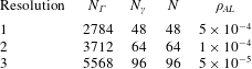
. We refined the spatio-temporal resolution until the trajectories converged (see appendix C for the details of the convergence study). We used the converged discretization for the pillars and the converged temporal resolution in all our simulations. As the row-shift fraction changes, the number of columns and hence the size of the exterior wall change. In order to maintain the same grid quality in all our simulations, we adjusted the discretization of the exterior wall depending on
 $\unicode[STIX]{x1D716}$
.
We also show that our model is not sensitive to the lateral position or inclination angle at which the RBCs are initialized (see figure 20 for the results).
2.4 Validation
The separation of rigid spherical particles using a DLD device of circular pillars is well understood (Huang et al.
Reference Huang, Cox, Austin and Sturm2004; Inglis et al.
Reference Inglis, Davis, Austin and Sturm2006; Zhang et al.
Reference Zhang, Henry, Gompper and Fedosov2015). An empirical formula for the critical particle size is given as a function of the gap size
 $G$
and row-shift fraction
 $\unicode[STIX]{x1D716}$
(Davis Reference Davis2008)
 $$\begin{eqnarray}\displaystyle D_{c}=1.4G\unicode[STIX]{x1D716}^{0.48}, & & \displaystyle\end{eqnarray}$$
where
 $D_{c}$
is the critical diameter. Particles with diameters
 $D>D_{c}$
displace while those with
 $D<D_{c}$
zig-zag. In order to validate our DLD model we simulated the separation of rigid spherical particles. We considered four different DLD devices with the same gap
 $G=10~\unicode[STIX]{x03BC}\text{m}$
and different row-shift fractions
 $\unicode[STIX]{x1D716}\in \{0.05,0.1,0.167,0.25\}$
. We had 8 rigid circular particles with
 $D=\{2,3,4,5,6,7,8,8.5\}~\unicode[STIX]{x03BC}\text{m}$
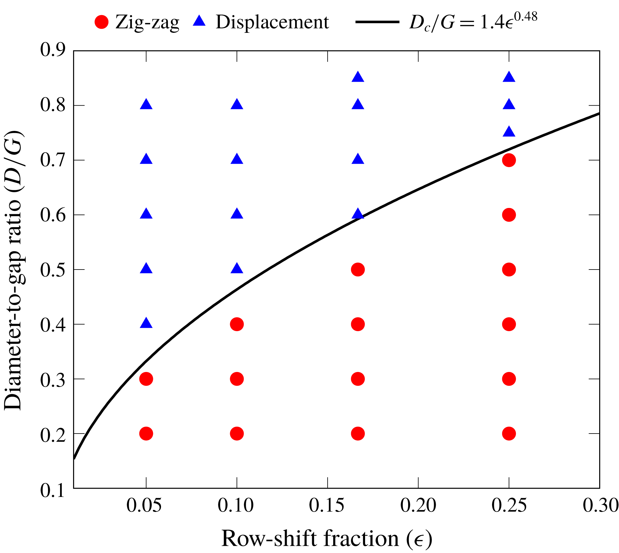
flowing through these DLD devices. We observed the trajectories of the particles and determined whether they zig-zag or displace in one period. We present the results of the validation study in figure 6. We also plot the line for the ratio of the critical diameter to the gap
 $D_{c}/G$
given by the empirical formula (2.10). As expected, the particles with diameters greater than
 $D_{c}$
(above the line in figure 6) displace while those with smaller diameters (below the line) zig-zag. Our numerical results agree well with the experimental results (Inglis et al.
Reference Inglis, Davis, Austin and Sturm2006; Davis Reference Davis2008). This validates our 2-D model and proves that it can capture the underlying physics of the particle separation in DLD devices.
Phase diagram for rigid spherical particles in DLD devices of circular pillars as a function of the row-shift fraction
 $\unicode[STIX]{x1D716}$
and the particle diameter-to-gap ratio
 $D/G$
. We also plot the critical particle size given by the empirical formula (2.10) (solid black line). Particles having greater diameters than the critical diameter displace while those with smaller diameters zig-zag. We show the zig-zagging and displacing particles with filled red circles and blue triangles, respectively. Our numerical results agree well with experimental results (Inglis et al.
Reference Inglis, Davis, Austin and Sturm2006; Davis Reference Davis2008).

Remark. In our simulations we consider the transport of the particles at high Péclet numbers (i.e.
 $Pe\gg 1$
, the transport is advection dominated). Therefore, the mixed mode, which is an irregular alternation between zig-zag and displacement modes (Huang et al.
Reference Huang, Cox, Austin and Sturm2004; Kulrattanarak et al.
Reference Kulrattanarak, van der Sman, Schröen and Boom2011; Zhang et al.
Reference Zhang, Henry, Gompper and Fedosov2015), is not observed in our study. This mode occurs as a result of diffusion of particles between different streamlines.
2.5 Dimensionless numbers
In this section, we summarize the parameter values that we will use in our experiments in § 4. The parameter selection is related to separating normal and abnormal RBCs based on differences in their deformability. The deformability of a cell depends on the cell’s membrane elasticity, cytoplasmic viscosity and the imposed flow. These can be combined to a single non-dimensional number, the capillary number:
 $$\begin{eqnarray}\displaystyle C_{a}=\frac{\unicode[STIX]{x1D702}_{out}R_{eff}^{3}}{\unicode[STIX]{x1D705}_{b}}\frac{U_{max}}{G/2}, & & \displaystyle\end{eqnarray}$$
where
 $\unicode[STIX]{x1D702}_{out}$
is the viscosity of the exterior fluid,
 $R_{eff}$
is the effective radius of the cell (
 $R_{eff}=\sqrt{A/\unicode[STIX]{x03C0}}$
in which
 $A$
is the area enclosed by the cell),
 $U_{max}$
is the maximum velocity of the unperturbed Poiseuille flow in a gap (2.9),
 $\unicode[STIX]{x1D705}_{b}$
is the bending stiffness and
 $G$
is the gap width. The higher the capillary number is, the more deformable the cell is. Typically, the bending stiffness and cell thickness (corresponding to its effective size in deep devices) for a healthy red blood cell are
 $\unicode[STIX]{x1D705}_{b}=1\times 10^{-19}~\text{Nm}$
(Suresh et al.
Reference Suresh, Spatz, Mills, Micoulet, Dao, Lim, Beil and Seufferlein2005; Tomaiuolo Reference Tomaiuolo2014) and
 $R_{eff}=2.5~\unicode[STIX]{x03BC}\text{m}$
(Popel & Johnson Reference Popel and Johnson2005), respectively. The viscosity of the blood plasma is
 $\unicode[STIX]{x1D702}_{out}=1.2~\text{mPa}~\text{s}$
. For the reported experiments (McGrath et al.
Reference McGrath, Jimenez and Bridle2014), the order of
 $U_{max}$
ranges between
 $10~\unicode[STIX]{x03BC}\text{m}~\text{s}^{-1}$
and
 $10~\text{mm}~\text{s}^{-1}$
in the DLD devices used to separate the blood components. In these devices the gap width is of the order of
 $O(1~\unicode[STIX]{x03BC}\text{m})$
, which is also the size in our study. Based on those typical values, the capillary number for a healthy RBC is
 $C_{a}\in [0.0375,375]$
. For the diseased RBC the capillary number decreases to its 1/10 since the stiffness increases 10-fold (Suresh et al.
Reference Suresh, Spatz, Mills, Micoulet, Dao, Lim, Beil and Seufferlein2005). Therefore, we consider capillary numbers in the range of
 $[0.0038,37.5]$
. We set the capillary number by adjusting the bending stiffness
 $\unicode[STIX]{x1D705}_{b}$
only and fix all other parameters.
The dimensionless number quantifying the cytoplasmic viscosity of an RBC
 $\unicode[STIX]{x1D702}_{in}$
is the viscosity contrast
 $$\begin{eqnarray}\displaystyle \unicode[STIX]{x1D708}=\frac{\unicode[STIX]{x1D702}_{in}}{\unicode[STIX]{x1D702}_{out}}. & & \displaystyle\end{eqnarray}$$
An RBC’s cytoplasmic viscosity is a nonlinear function of the mean corpuscular haemoglobin concentration (MCHC), which is the concentration of the haemoglobin per unit volume of a RBC (Aouane et al.
Reference Aouane, Thiebaud, Benyoussef, Wagner and Misbah2014). The viscosity varies from one cell to the other even within the same organism due to age because the MCHC increases as the RBC gets older. For a young red blood cell the MCHC is around
 $32~\text{g}~\text{dl}^{-1}$
, which results in
 $\unicode[STIX]{x1D702}_{in}=5{-}7~\text{mPa}~\text{s}$
, i.e. the viscosity contrast is
 $\unicode[STIX]{x1D708}=4{-}6$
. If the MCHC increases to
 $40~\text{g}~\text{dl}^{-1}$
, the viscosity increases almost fourfold (Chien Reference Chien1987; Mohandas & Gallagher Reference Mohandas and Gallagher2008). Viscosity contrast is inversely proportional to cell’s deformability. So, the smaller the viscosity contrast is, the more deformable the cell is. We consider
 $\unicode[STIX]{x1D708}\in [0.1,100]$
in our study and set the viscosity contrast by changing the interior viscosity
 $\unicode[STIX]{x1D702}_{in}$
.
Following Vlahovska & Gracia (Reference Vlahovska and Gracia2007) we define a time scale as the deformation time scale driven by the imposed flow, which is the inverse of the shear gradient in a gap
 $$\begin{eqnarray}\displaystyle \unicode[STIX]{x1D70F}=\frac{G/2}{U_{max}}. & & \displaystyle\end{eqnarray}$$
We have already presented the geometry of our DLD model in § 2.2. The third dimensionless number is the row-shift fraction
 $\unicode[STIX]{x1D716}$
of the DLD device. We adjust
 $\unicode[STIX]{x1D716}$
by changing the row shift
 $\unicode[STIX]{x0394}\unicode[STIX]{x1D706}$
and the other DLD parameters remain the same.
3 Results
First, we investigate the effects of the capillary number in § 3.1 and the viscosity contrast in § 3.2 on the dynamics of red blood cells in deep devices. Then in § 3.3, we present phase diagrams for the transport modes as a function of the capillary number
 $C_{a}$
, the viscosity contrast
 $\unicode[STIX]{x1D708}$
and the row-shift fraction
 $\unicode[STIX]{x1D716}$
. Finally, we study the cell separation in the flow of dense RBC suspensions through the DLD devices in § 3.4.
3.1 Effects of capillary number
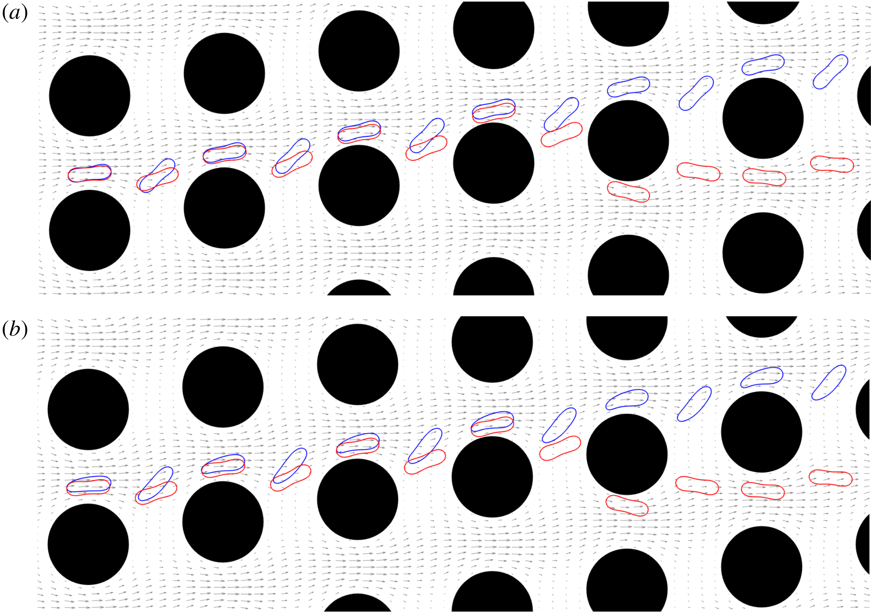
Superimposed snapshots from the simulations of RBCs having different capillary numbers
 $C_{a}$
and the unperturbed velocity field (shown with grey arrows). Here, we initialize the cells at the same position and simulate them separately. We then superimpose the snapshots taken when the cells are in the gaps and between two consecutive gaps. The viscosity contrast and the row-shift fraction in these simulations are the same,
 $\unicode[STIX]{x1D708}=1$
and
 $\unicode[STIX]{x1D716}=0.1667$
, respectively. In (a) we compare the dynamics of two stiff cells with
 $C_{a}=0.034$
(red) and
 $C_{a}=0.34$
(blue). While the stiffer cell (red) zig-zags, the softer one (blue) displaces. In (b) we keep the stiffest cell (
 $C_{a}=0.034$
, red one) but replace the softer one with an even a softer cell (
 $C_{a}=34$
, blue one). Again, the softer cell (blue) displaces.

We performed simulations of a single RBC flowing through DLD with the capillary numbers
 $C_{a}=(0.034,0.34,34)$
. The viscosity contrast for these cells is
 $\unicode[STIX]{x1D708}=1$
. We considered only one device with row-shift fraction
 $\unicode[STIX]{x1D716}=0.1667$
. We present the superimposed snapshots from these simulations in figure 7 together with the unperturbed velocity field (shown with grey arrows). The snapshots are taken when the cells are in the gaps and between the consecutive gaps. The cells are initialized at the same location and have effective radius
 $R_{eff}=2.4~\unicode[STIX]{x03BC}\text{m}$
.
In figure 7(a) we compare two stiff cells: the red one (
 $C_{a}=0.034$
) is stiffer than the blue one (
 $C_{a}=0.34$
). While the stiffer one zig-zags, the softer one displaces. Then, in (b), we replace the softer one with an even softer cell having
 $C_{a}=34$
. The softer cell again displaces. We now discuss our observations from these simulations. In the gaps, the stiff cell (low
 $C_{a}$
) does not deform as much as the soft one does (high
 $C_{a}$
). The stiff cell behaves like a rigid particle and moves closer to the pillars than the softer cell does. A rigid spherical particle with a diameter less than
 $6~\unicode[STIX]{x03BC}\text{m}$
zig-zags in a device with
 $\unicode[STIX]{x1D716}=0.1667$
as shown in § 2.4. Since the cell’s effective size is less than this critical size, it zig-zags. There are several other differences in the cells’ behaviours depending on their stiffness. The softer cells have an asymmetry in their shape while they are passing through a gap. They have a thick head and a thin tail in the gaps (this is more apparent for
 $C_{a}=34$
) while the stiff cell maintains its symmetric relaxed shape. The asymmetry in the soft cells’ shapes and the shear gradient in the gap lead the soft cells to have a higher inclination angle with respect to the main flow direction than the stiff ones while they are moving towards the region between two consecutive gaps.
The positive inclination angle with respect to the flow direction and the shear gradient together result in a phenomenon called cell migration, which has been extensively studied in the literature (Goldsmith & Mason Reference Goldsmith and Mason1961; Olla Reference Olla1997; Vlahovska & Gracia Reference Vlahovska and Gracia2007; Coupier et al.
Reference Coupier, Kaoui, Podgorski and Misbah2008; Danker et al.
Reference Danker, Vlahovska and Misbah2009; Messlinger et al.
Reference Messlinger, Schmidt, Noguchi and Gompper2009; Ghigliotti et al.
Reference Ghigliotti, Rahimian, Biros and Misbah2011). A cell placed near a wall migrates away from the wall in confined Poiseuille flow or shear flow due to its positive inclination with respect to the wall and the shear gradient. Here, the flow in DLD resembles the Poiseuille flow (confined flow in the gaps and almost free flow between the gaps). Therefore, a cell with positive inclination moves away from the pillars and if it is sufficiently far from the pillars (i.e. it is out of the adjacent stream swapping a lane), it displaces. As the inclination increases, it moves even farther away from the pillars. Figure 7 shows that as the cell becomes softer, its inclination angle increases. That is, the cells with
 $C_{a}=(0.34,34)$
have higher inclination angles right after the first gap than the one with
 $C_{a}=0.034$
. The softer cells maintain this positive inclination and stay away from the pillars. Additionally, the cell with
 $C_{a}=34$
has a higher inclination angle than the one with
 $C_{a}=0.34$
and moves farther away from the pillars than the one with
 $C_{a}=0.34$
(see the gaps in both figures). Zhang et al. (Reference Zhang, Henry, Gompper and Fedosov2015) also observed that RBCs stay away from pillars with square cross-sections and attributed this behaviour to the fact that the flow resembles a confined Poiseuille flow and hence the cells migrate. We discuss the similarities between the flow in DLD and confined Poiseuille flow in § 4 and compare the cells’ inclination angles for various capillary numbers and viscosity contrasts.
3.2 Effects of viscosity contrast
Superimposed snapshots from the simulations of RBCs having different viscosity contrasts
 $\unicode[STIX]{x1D708}$
and the unperturbed velocity field (shown with grey arrows). Here, we initialize the cells at the same position and simulate them separately. We then superimpose the snapshots taken when the cells are in the gaps and between two consecutive gaps. The capillary number and the row-shift fraction in these simulations are
 $C_{a}=3.41$
and
 $\unicode[STIX]{x1D716}=0.1667$
, respectively. In (a) we compare the dynamics of the less viscous cells with
 $\unicode[STIX]{x1D708}=1$
(blue) and
 $\unicode[STIX]{x1D708}=2$
(red). Both of these cells displace. In (b) we compare the cell having
 $\unicode[STIX]{x1D708}=1$
with that with
 $\unicode[STIX]{x1D708}=5$
. The cell with
 $\unicode[STIX]{x1D708}=5$
corresponds to a healthy RBC and it zig-zags.

In the previous section, we considered cells with no viscosity contrast. We now want to investigate how the cells’ dynamics in DLD depend on their viscosity contrast. We performed simulations of a single RBC flowing through DLD with the viscosity contrast values
 $\unicode[STIX]{x1D708}=(1,2,5)$
. The capillary number for these cells is
 $C_{a}=3.41$
. We considered the same device as in the previous section, i.e. the row-shift fraction is
 $\unicode[STIX]{x1D716}=0.1667$
. We present the superimposed snapshots from these simulations in figure 8 together with the unperturbed velocity field (shown with grey arrows). Here, the snapshots are taken when the cells are passing through the gaps and between two consecutive gaps. The cells are initialized at the same location and have an effective radius
 $R_{eff}=2.4~\unicode[STIX]{x03BC}\text{m}$
.
The RBCs here have a moderate capillary number so they can be considered more deformable than the stiff cells in the previous section. In figure 8(a) we compare cells with no viscosity contrast (i.e.
 $\unicode[STIX]{x1D708}=1$
, blue) and with the viscosity contrast
 $\unicode[STIX]{x1D708}=2$
(red). Here, both cells displace. As observed in the previous section, both cells have thick heads and thin tails in the gaps. Additionally, they have positive inclination angle with respect to the flow direction in the gaps. Their inclination angle increases when they are between two consecutive gaps. Then, due to this asymmetry and the shear gradient, they migrate away from the pillars. Since they stay sufficiently away from the pillars, they displace. In figure 8(b) we compare a cell having no viscosity contrast with one having a viscosity contrast
 $\unicode[STIX]{x1D708}=5$
. The cell with
 $\unicode[STIX]{x1D708}=5$
at this capillary number might be considered a healthy cell and it zig-zags in this device. Although the more viscous cell (red one) still maintains a positive inclination with respect to the flow direction, this angle is lower than one with no viscosity contrast (see the cells right after the first gap). As a result of having smaller inclination angle, the more viscous cell cannot remain as far away from the pillars as the cell with no viscosity contrast does (see the cells in the third gap for instance). So the more viscous cell eventually swaps a lane.
It is known that the cells show either tank-treading (moving with the same inclination) or tumbling (moving while rotating around its axis) depending on its viscosity contrast and capillary number. In free shear flows, the cells with
 $\unicode[STIX]{x1D708}=5$
tumble (Kantsler & Steinberg Reference Kantsler and Steinberg2006). So one might expect the same cell to tumble in DLD as well. However, the confinement reduces the inclination angle of a tank-treading cell and also delays the tumbling. It turns out that tumbling does not occur for the confinement level we have in the gaps in this study, which is
 $2R_{eff}/G=0.48$
(see Kaoui, Krüger & Harting (Reference Kaoui, Krüger and Harting2012)). That is why the cells in DLD always maintain a positive inclination and the inclination decreases as the viscosity contrast increases. We discuss how the inclination angle varies with viscosity contrast in both confined Poiseuille flows and DLD in detail in § 4.
Remark. Another consequence of aging besides increasing viscosity contrast is that RBCs lose surface area (arc-length in two dimensions) (Mohandas & Gallagher Reference Mohandas and Gallagher2008), so the reduced area increases. In shear and Poiseuille flows, the cell’s migration velocity and inclination angle decrease as the reduced area increases. In the circular limit (a reduced area of 1), the cell does not deform and migrate. Since the cell dynamics in DLD is different to that in simpler flows, how the transport modes depend on the reduced area needs to be investigated.
In order to shed some light on this issue we performed simulations of cells with
 $C_{a}=3.41$
and
 $\unicode[STIX]{x1D708}=(1,10)$
, and DLD devices with
 $\unicode[STIX]{x1D716}=(0.1,0.125,0.167)$
. We increased the reduced area from 0.65 to 0.75, 0.85 and 0.95. Recall that the reduced area is 0.65 for the other experiments in the study. We found that the cell with
 $\unicode[STIX]{x1D708}=1$
displaces for all of the
 $\unicode[STIX]{x1D716}$
values regardless of its reduced area. The cell with
 $\unicode[STIX]{x1D708}=10$
zig-zags for these
 $\unicode[STIX]{x1D716}$
values when the reduced area is 0.65. For greater reduced areas the cell tumbles for
 $\unicode[STIX]{x1D716}=(0.1,0.125)$
and displaces while it still zig-zags for
 $\unicode[STIX]{x1D716}=0.1667$
. Our conclusion is that the cell’s transport mode in DLD can change with its reduced area depending on the row-shift fraction
 $\unicode[STIX]{x1D716}$
and the viscosity contrast
 $\unicode[STIX]{x1D708}$
. This shows that a more detailed study of the reduced area effects is required, although such a study is beyond the scope of our work.
3.3 Phase diagrams
We performed an analysis in order to determine how the cells’ transport modes depend on their capillary number
 $C_{a}$
, viscosity contrast
 $\unicode[STIX]{x1D708}$
and the DLD’s row-shift fraction
 $\unicode[STIX]{x1D716}$
. We obtained three phase diagrams for the transport modes of a single cell in DLD which are described below.
(i)
$\unicode[STIX]{x1D716}$
versus
$C_{a}$
(figure 9
a): we fixed the viscosity contrast to
$\unicode[STIX]{x1D708}=10$
and performed simulations for
$\unicode[STIX]{x1D716}\in [0.0625,2.5]$
and
$C_{a}\in [3.4\times 10^{-3},3.4\times 10^{-1}]$
.(ii)
$\unicode[STIX]{x1D716}$
versus
$\unicode[STIX]{x1D708}$
(figure 9
b): we fixed the capillary number to
$C_{a}=3.4\times 10^{-1}$
and performed simulations for
$\unicode[STIX]{x1D716}\in [0.0625,2.5]$
and
$\unicode[STIX]{x1D708}\in [1,10]$
.(iii)
$\unicode[STIX]{x1D708}$
versus
$C_{a}$
(in figure 10): we fixed the row-shift fraction to
$\unicode[STIX]{x1D716}=0.1667$
(figure 10
a) and
$\unicode[STIX]{x1D716}=0.1$
(figure 10
b). Then, we performed simulations for
$\unicode[STIX]{x1D708}=(1,2,5,8,10,100)$
and
$C_{a}=[3.4\times 10^{-2},3.4\times 10^{3}]$
.


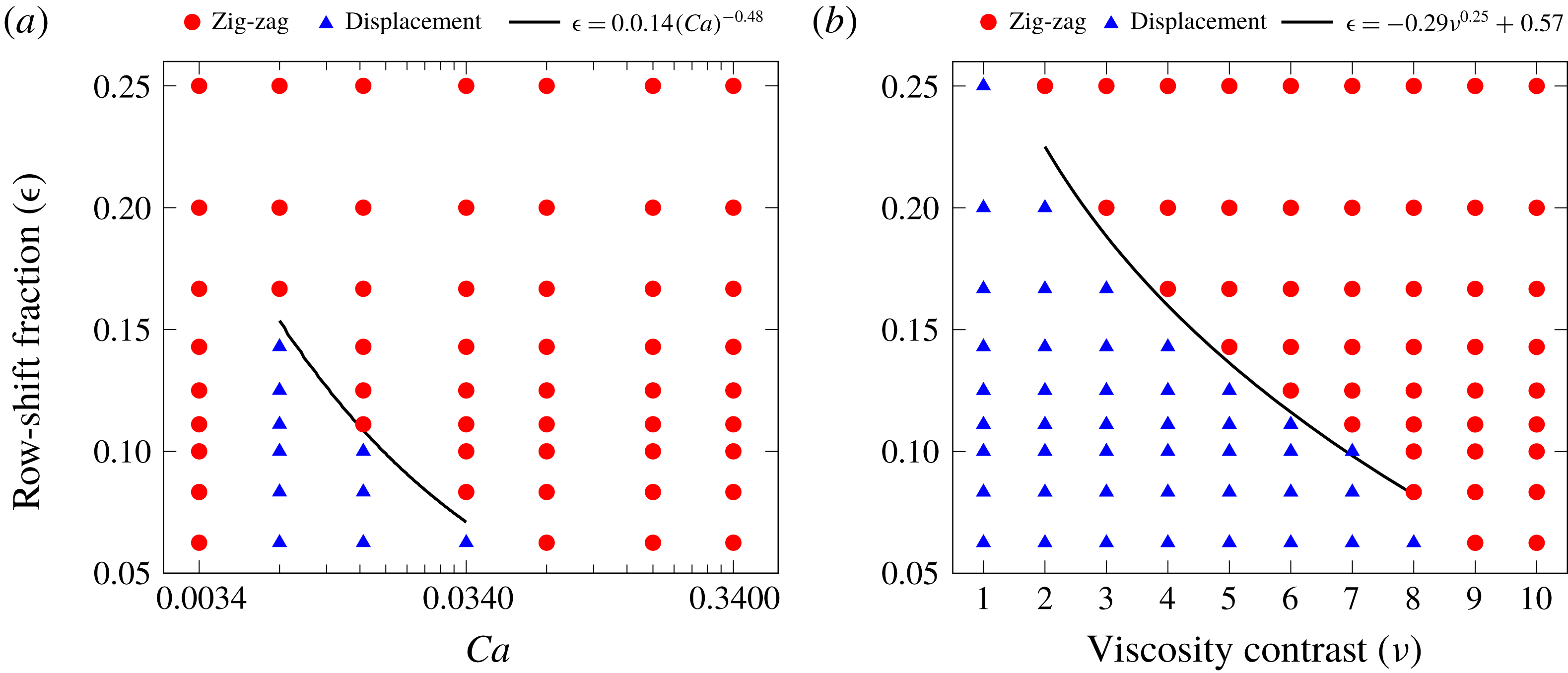
Phase diagrams for the transport modes as a function of the capillary number
 $C_{a}$
and row-shift fraction
 $\unicode[STIX]{x1D716}$
with
 $\unicode[STIX]{x1D708}=10$
(a) and as a function of the viscosity contrast
 $\unicode[STIX]{x1D708}$
and
 $\unicode[STIX]{x1D716}$
with
 $C_{a}=0.34$
(b). Red circles and blue triangles indicate zig-zagging and displacing cells, respectively. The solid line in (a) corresponds to (3.1a
) and the one in (b) corresponds to (3.1b
). These equations approximate the separation between two transport modes.

We first discuss the phase diagrams for
 $C_{a}$
versus
 $\unicode[STIX]{x1D716}$
and
 $\unicode[STIX]{x1D708}$
versus
 $\unicode[STIX]{x1D716}$
in figure 9. Panel (a) shows that as the capillary number increases, the transport mode shifts from zig-zag to displacement and for larger capillary numbers it again shifts to zig-zag. This is not observed for (b). For low viscosity contrasts the cell displaces and as the viscosity contrast increases, the transport mode shifts to zig-zag. Since the rigidity of a cell increases as its viscosity contrast increases or its capillary number decreases, one would expect the same dynamics as a cell becomes rigid. Our results agree with this expectation. The phase diagrams show that a cell has the same transport mode in the limit of low capillary number and high viscosity contrast. This transport mode is zig-zag. This is reasonable because a very rigid cell behaves like a rigid spherical particle with a diameter equal to the cell’s thickness
 ${\approx}2.5~\unicode[STIX]{x03BC}\text{m}$
(i.e. it cannot migrate and its effective size is
 ${\approx}2.5~\unicode[STIX]{x03BC}\text{m}$
) and the critical particle size given by (2.10) for the row-shift fractions considered here is greater than the cell’s thickness (i.e.
 $D_{c}=3.7~\unicode[STIX]{x03BC}\text{m}$
). So the rigid cell zig-zags. The reason why we observe different transport modes depending on the capillary number and viscosity contrast is that a cell’s inclination angle depends on these parameters and it migrates some amount which depends on its inclination angle as observed in the previous sections. However, the rigid cell does not migrate. The curves separating the transport modes in these figures are given by a power law (3.1a
) (a) and (3.1b
) (b).
 $$\begin{eqnarray}\displaystyle & \displaystyle \unicode[STIX]{x1D716}=0.014{C_{a}}^{-0.48}, & \displaystyle\end{eqnarray}$$
 $$\begin{eqnarray}\displaystyle & \displaystyle \unicode[STIX]{x1D716}=-0.29\unicode[STIX]{x1D708}^{0.25}+0.26. & \displaystyle\end{eqnarray}$$
 $R^{2}$
is the coefficient of determination, which indicates the goodness of a fit. The curve fits (3.1a
) and (3.1b
) have
 $R^{2}=0.92$
and
 $R^{2}=0.91$
, respectively.
Phase diagrams for the transport modes as a function of the viscosity contrast
 $\unicode[STIX]{x1D708}$
and capillary number
 $C_{a}$
for the row-shift fractions
 $\unicode[STIX]{x1D716}=0.1667$
and
 $\unicode[STIX]{x1D716}=0.1$
. Red circles and blue triangles indicate zig-zagging and displacing cells, respectively.

Figure 10 indicates how the transport mode depends on the capillary number and viscosity contrast for a fixed row-shift fraction. Here, (a) shows the row-shift fraction
 $\unicode[STIX]{x1D716}=0.1667$
and (b)
 $\unicode[STIX]{x1D716}=0.1$
. We observe that in DLD with higher row-shift fraction cells zig-zag more. That is, under the same conditions (
 $\unicode[STIX]{x1D708}$
and
 $C_{a}$
) a cell zig-zags for high
 $\unicode[STIX]{x1D716}$
and displaces for low
 $\unicode[STIX]{x1D716}$
. For example, the mode is zig-zag in
 $\unicode[STIX]{x1D716}=0.1667$
and displacement in
 $\unicode[STIX]{x1D716}=0.1$
for
 $\unicode[STIX]{x1D708}=5$
and
 $C_{a}=3.4\times 10^{-1}$
. The reason is as the row-shift fraction increases, the width of the adjacent stream (and hence the critical size) increases. In order for a cell to displace for that case higher migration velocity (i.e. higher inclination angle) is required. That is why, for the same viscosity contrasts and capillary numbers, figure 10(a) (
 $\unicode[STIX]{x1D716}=0.1667$
) has more zig-zagging cases than figure 10(b) (
 $\unicode[STIX]{x1D716}=0.1$
). For
 $\unicode[STIX]{x1D716}=0.1667$
, only the cells with viscosity contrasts
 $\unicode[STIX]{x1D708}=(1,2)$
displace if their capillary number is greater than
 $3.4\times 10^{-2}$
. So the viscosity contrast based separation is possible for these cells. However, the capillary number based separation is only possible for viscosity contrasts
 $\unicode[STIX]{x1D708}=(1,2)$
and for very low capillary numbers. For
 $\unicode[STIX]{x1D716}=0.1$
, the transport mode shifts from zig-zag to displacement and then to zig-zag again as the capillary number increases for the viscosity contrast
 $\unicode[STIX]{x1D708}\geqslant 5$
. So, the separation based on the capillary number is possible for higher capillary numbers than it is for
 $\unicode[STIX]{x1D716}=0.1667$
.
3.4 Breakdown of DLD efficiency in dense suspensions
The DLD theory is developed for dilute suspensions assuming that the unperturbed velocity field (in the absence of particles) is not distorted when the particles are present. So that the particle–pillar interactions result in deterministic particle trajectories and hence separation. Additionally, the phase diagrams for deformability-based RBC separation in our study and the literature (Quek et al.
Reference Quek, Le and Chiam2011; Krüger et al.
Reference Krüger, Holmes and Coveney2014) are obtained simulating a single particle in a DLD device. As the suspensions become denser, the particle–particle interactions dominate the particle–pillar interactions and separation may not occur any longer because particles with the same properties are not in the same transport modes (Vernekar & Krüger Reference Vernekar and Krüger2015). The DLD efficiency for dense suspensions is of interest because the use of dense suspensions would reduce the operation time and remove the pre-treatment (such as dilution) requirement. Inspired by Vernekar & Krüger (Reference Vernekar and Krüger2015) we are interested in failure of the transport modes in dense suspensions of RBCs in deep devices. In order to explain the failure, let us consider a single RBC with a certain viscosity contrast and capillary number and suppose that this RBC displaces in its dilute suspension for a certain row-shift fraction. When a dense suspension of this RBC flows in the same device, not all of the cells displace. This is called failure in the displacement mode. Similarly, we define failure in the zig-zag mode, too. Vernekar & Krüger (Reference Vernekar and Krüger2015) performed 3-D simulations of the flow of dense RBC suspensions in shallow devices for various capillary numbers, row-shift fractions and volume fractions under a constant viscosity contrast of
 $\unicode[STIX]{x1D708}=5$
. The key findings of their study are as follows.
(i) As the volume fraction increases for the same row-shift fraction and capillary number, more RBCs zig-zag independent of the transport mode of a single RBC under the same conditions. So the displacement mode is more prone to failure than the zig-zag mode. Consequently, it is easier to separate large particles such as white blood cells from dense suspensions of RBCs than the small particles (e.g. platelets), since the small particles also zig-zag like the RBCs.
(ii) At the same volume fraction and capillary number, increasing the row-shift fraction reduces the failure rate of the displacement mode in one period of the device. However, a DLD device with small row-shift fraction must be long enough to have significant lateral separation between displacing and zig-zagging particles at the end. This requires using many periods of the device, which increases the failure rate in the overall device. Therefore, the use of small row-shift fractions does not prevent the breakdown.
Inglis et al. (Reference Inglis, Lord and Nordon2011) also made the same observations in their experimental study.
Frames from a simulation of a dense RBC suspension for the row-shift fraction
 $\unicode[STIX]{x1D716}=0.1667$
. The suspension has a volume fraction of 15 %. All RBCs in the suspension have the same capillary number
 $C_{a}=0.34$
and viscosity contrast
 $\unicode[STIX]{x1D708}=1$
. The phase diagram in figure 9 shows that a single RBC with these parameters displaces. In its dense suspension, however, only 30 % of the RBCs displace.
 $\unicode[STIX]{x1D70F}$
is the time scale defined as the inverse of the shear gradient in a gap, i.e.
 $\unicode[STIX]{x1D70F}=G/2U_{max}$
. See figure 12 for the statistics of the dense suspensions.

Here, we performed numerical simulations of dense suspensions in deep devices. We first considered RBCs with two different capillary numbers
 $C_{a}=(0.0034,0.34)$
but a fixed viscosity contrast of
 $\unicode[STIX]{x1D708}=10$
for the row-shift fractions
 $\unicode[STIX]{x1D716}$
 $=$
(0.0833, 0.125, 0.1667). Secondly, we conducted the same experiments with two different viscosity contrasts
 $\unicode[STIX]{x1D708}=(1,10)$
but a fixed capillary number of
 $C_{a}=0.34$
. As in the previous sections, we observed the transport mode in one period of the device. We filled the middle lane of the device with randomly initialized RBCs. Then, as the simulation went on, we initialized new RBCs at a random lateral position at the leftmost point of the device randomly in time. We ran the simulations until 100 RBCs in total travelled to the end of the device. We define and calculate the volume fraction as follows. Considering a circle centred at each cell’s centre with a diameter equal to the cell’s arc-length, we compute the so-called local volume fraction which is the ratio of the area occupied by the cells in the circle to the area of the circle. Finally, taking the average of the local volume fraction over time and cells delivers the volume fraction of the simulation. In figure 11 we present the frames from the simulation of RBCs with
 $C_{a}=0.34$
and
 $\unicode[STIX]{x1D708}=1$
for the row-shift fraction
 $\unicode[STIX]{x1D716}=0.1667$
. We report the numbers of zig-zagging and displacing RBCs in the dense suspensions in figure 12. The dense suspensions in our simulations had volume fractions of 15 %–20 %. We found that one RBC interacts with approximately two to three other RBCs on average throughout its motion in our simulations. The statistics in figure 12 agree well with the findings of Inglis et al. (Reference Inglis, Lord and Nordon2011) and Vernekar & Krüger (Reference Vernekar and Krüger2015). We summarize our results as follows.
(i) The displacement mode due to either viscosity contrast or capillary number is more susceptible to failure. That is, more than 50 % of the RBCs in a dense suspension zig-zag for the two largest row-shift fractions (the first two columns in figure 12) while the transport mode of a RBC with the same properties is displaced in its dilute suspension (see the first and the last rows). Only 15–20 % of the zig-zagging RBCs fail to zig-zag (see the second row).
(ii) For the smaller row-shift fractions (from left to right in the same figure), the breakdown is less pronounced. Only 25 % of the displacing RBCs zig-zag in a dense suspension for the smallest row-shift fraction (see the last column).
Breakdown of the transport modes in dense RBC suspensions. We performed simulations of a single RBC (dilute suspension) and multiple RBCs (dense suspension) for the row-shift fractions
 $\unicode[STIX]{x1D716}=(0.083,0.125,0.1667)$
. We considered RBCs with the capillary numbers
 $C_{a}=(0.0034,0.34)$
and viscosity contrasts
 $\unicode[STIX]{x1D708}=(1,10)$
. The dense suspensions have volume fractions of 15 to 20 %. We present the histogram plots showing the numbers of zig-zagging and displacing RBCs (out of 100). In the dilute suspensions, a single RBC either zig-zags or displaces. Therefore, we observe either 100 % zig-zagging or displacement in the dilute suspensions, whereas in dense suspensions the same RBCs are not in the same transport modes. Results in each column are for different row-shift fractions (decreasing from left to right) and those at each row have different combinations of
 $C_{a}$
and
 $\unicode[STIX]{x1D708}$
.

4 Discussion
In this section, we investigate the underlying mechanism for the RBC separation depending on the capillary number and viscosity contrast in deep DLD devices. Since the flow in DLD resembles free shear flow (between the vertical gaps) and confined Poiseuille flow (in the vertical gaps), we compare the cell dynamics in DLD with that in these simpler flows. We present the similarities and seek to understand if these simpler set-ups can be used to predict whether a cell displaces or zig-zags in a particular DLD device.
4.1 Free shear flow
The results in § 3 show that cells having high positive inclination angles with respect to the flow direction displace and those having lower inclination angles zig-zag. This is a result of a positive inclination angle and shear gradient, which lead a cell to migrate away from the pillars. A cell’s inclination angle depends on its capillary number and viscosity contrast. In free shear flow, cells tilt to a certain angle and move with that angular orientation for low capillary numbers and viscosity contrasts. This motion is called tank-treading. For high capillary numbers and viscosity contrasts, cells do not have such an angular orientation and tumble (Kantsler & Steinberg Reference Kantsler and Steinberg2006; Misbah Reference Misbah2006). In free shear flow, tank-treading cells migrate from high shear rate regions to low shear rate regions while tumbling cells do not migrate (Olla Reference Olla1997; Vlahovska & Gracia Reference Vlahovska and Gracia2007; Messlinger et al.
Reference Messlinger, Schmidt, Noguchi and Gompper2009). Henry et al. (Reference Henry, Holm, Zhang, Beech, Tegenfeldt, Fedosov and Gompper2016) investigated the sorting of cells depending on this cell dynamics and concluded that tank-treading at the viscosity contrast
 $\unicode[STIX]{x1D708}=1$
results in displacement and tumbling usually leads to zig-zag. They observed tumbling between the gaps right before a cell zig-zags, which we also observed for some cases. It must be noted that tumbling does not occur in the gaps in DLD due to the confinement (Kaoui et al.
Reference Kaoui, Krüger and Harting2012).
We investigate whether the conditions (the capillary number and the viscosity contrast) causing cells to tank-tread in free shear flow lead cells to displace in DLD for any row-shift fraction. In other words, we investigate whether the conditions causing cells to tumble in free shear flow lead cells to zig-zag in DLD for any row-shift fraction. If this is true, then we can estimate the cell dynamics in DLD by simulating cells in a simpler free shear flow. However, as we can see in figure 10, a cell tank-treading in a free shear flow does not necessarily displace in DLD flow for the same capillary number and the viscosity contrast. For example, a cell that tumbles for
 $\unicode[STIX]{x1D708}=5$
and
 $C_{a}=O(10)$
in free shear flow displaces in the DLD for
 $\unicode[STIX]{x1D716}=0.1$
but zig-zags for
 $\unicode[STIX]{x1D716}=0.1667$
. The main reason that the dynamics in free shear flow cannot predict the transport mode in DLD is that the row-shift fraction information does not enter free shear flow. Additionally, the confinement in the gaps in DLD also affects this dynamics (Kaoui et al.
Reference Kaoui, Krüger and Harting2012).
4.2 Confined Poiseuille flow
The time-averaged inclination angles
 $\overline{\unicode[STIX]{x1D6FC}}$
and the migration velocities
 $\overline{v}_{mig}$
for a red blood cell in confined Poiseuille flow for various capillary numbers
 $C_{a}$
and viscosity contrasts
 $\unicode[STIX]{x1D708}$
. We considered a channel having the same confinement as the gaps in our DLD simulations. We initialized a cell below the centreline and let the cell migrate towards the centre.

Confining a cell by walls delays the cell’s transition from tank-treading to tumbling and can even avoid tumbling (Kaoui et al.
Reference Kaoui, Krüger and Harting2012). In order to incorporate the confinement effects into a simpler model, we now consider confined Poiseuille flow, which the flow in a DLD gap resembles, and we investigate the cell dynamics. We imposed a parabolic velocity similar to the flow in the DLD gaps on the side walls of a channel confined by two parallel walls. The width of this channel is the same as the width of the gap in our DLD simulations. Thus, the confinement is
 $\unicode[STIX]{x1D712}=2R_{eff}/G$
. The channel is centred at the origin and the cell is initialized at
 $y_{i}=-3G/10$
. We performed simulations of a cell for the same capillary numbers and viscosity contrasts that we considered in our DLD simulations, i.e.
 $C_{a}\in [3.41\times 10^{-2},3.41\times 10^{3}]$
and
 $\unicode[STIX]{x1D708}\in [1,10]$
. We let the cell migrate to
 $y_{f}=-G/10$
. We do not allow the cell to reach the centre because there it shows complex shape changes and equilibrium dynamics for this confinement (Aouane et al.
Reference Aouane, Thiebaud, Benyoussef, Wagner and Misbah2014). Additionally, the cell in DLD usually stays near the pillars not at the centre of the gaps. We measured the cell’s migration velocity
 $v_{mig}$
(i.e. velocity in the direction perpendicular to the flow direction) and inclination angle
 $\unicode[STIX]{x1D6FC}$
with respect to the walls at various lateral positions. We present the time-averaged inclination angles
 $\overline{\unicode[STIX]{x1D6FC}}$
and migration velocities
 $\overline{v}_{mig}$
for various capillary numbers
 $C_{a}$
and viscosity contrasts
 $\unicode[STIX]{x1D708}$
in figure 13. Panel (a) shows that the inclination angle varies less with the viscosity contrast for the lowest capillary number than higher capillary numbers. As the capillary number increases, the inclination angle increases. It also increases as the viscosity contrast decreases. So for lower viscosity contrasts and higher capillary numbers the inclination angle is higher. For
 $C_{a}\geqslant 10^{2}$
the inclination angle does not change significantly with
 $C_{a}$
. Additionally, the inclination angle increases monotonically with the capillary number for the viscosity contrasts
 $\unicode[STIX]{x1D708}=(1,2)$
but it does not change monotonically with the capillary number for the viscosity contrasts
 $\unicode[STIX]{x1D708}\geqslant 5$
. Panel (b) indicates that the average migration velocity parallels the average inclination angle. A cell migrates faster for lower viscosity contrasts. The migration velocity monotonically increases with the capillary number for the viscosity contrasts
 $\unicode[STIX]{x1D708}=(1,2)$
like the average inclination angle; however, this behaviour vanishes for viscosity contrasts
 $\unicode[STIX]{x1D708}\geqslant 5$
. Although the inclination angle still changes with
 $C_{a}$
for
 $C_{a}=O(1)$
, the migration velocity no longer changes significantly with
 $C_{a}$
for
 $C_{a}=O(1)$
. The reason might be the fact that the bending relaxation time scale dominates the time scale for shear flow for
 $C_{a}>1$
. Another observation is that a very rigid cell (i.e. the viscosity contrast
 $\unicode[STIX]{x1D708}=1000$
) also has a positive inclination with respect to the walls but the angle is an order of magnitude smaller than that for softer cells. This results in a very small migration velocity for the stiff cell. Overall, similar to the DLD flow examples, we do not observe tumbling for this confinement in confined Poiseuille flow, which agrees with Kaoui et al. (Reference Kaoui, Krüger and Harting2012).
Based on these results we expect that the transport mode in DLD depends on whether the degree of a cell’s inclination results in enough migration to keep the cell far away from the pillars. We now discuss how the inclination angle of a cell depends on
 $C_{a}$
,
 $\unicode[STIX]{x1D708}$
and
 $\unicode[STIX]{x1D716}$
in DLD flows and compare it with the above results for confined Poiseuille flows.
Inclination angles
 $\unicode[STIX]{x1D6FC}$
of RBCs for various viscosity contrasts
 $\unicode[STIX]{x1D708}$
at a fixed row-shift fraction
 $\unicode[STIX]{x1D716}=0.0625$
and for various row-shift fractions at a fixed viscosity contrast
 $\unicode[STIX]{x1D708}=1$
. The capillary number is the same for all the results,
 $C_{a}=0.34$
. The RBCs with
 $\unicode[STIX]{x1D708}=1,2,5$
displace and the one with
 $\unicode[STIX]{x1D708}=10$
zig-zags. The displacing RBCs have positive inclination angles alternating between two values (see a). The minimum angle is attained when the cell is in the gap and the cell reaches the maximum angle when it is between two gaps. The minimum and maximum angles reduce as the viscosity contrast increases. The maximum angle depends also on the row-shift fraction
 $\unicode[STIX]{x1D716}$
. As the row-shift fraction increases the maximum angle increases; however, the minimum angle does not change significantly (see b). The
 $x$
-coordinates are normalized by the lengths of the DLD devices
 $L$
.

We demonstrate how the inclination angle of a cell changes as the cell flows through a DLD device in figure 14. In (a), we vary the viscosity contrast
 $\unicode[STIX]{x1D708}$
by setting the capillary number to
 $C_{a}=0.34$
and row-shift fraction to
 $\unicode[STIX]{x1D716}=0.0625$
. In (b) we vary the row-shift fraction for a fixed capillary number
 $C_{a}=0.34$
and viscosity contrast
 $\unicode[STIX]{x1D708}=1$
. All these cells displace except the one with
 $\unicode[STIX]{x1D708}=10$
in (a). The displacing cells attain their minimum angles in the gaps and tilt to their maximum angles between two consecutive gaps. These maximum angles are
 $0.58$
rad for
 $\unicode[STIX]{x1D708}=1$
,
 $0.5$
rad for
 $\unicode[STIX]{x1D708}=2$
and
 $0.37$
rad for
 $\unicode[STIX]{x1D708}=5$
. These values are close to the steady inclination angles of the RBCs having these viscosity contrasts in an unbounded shear flow (Beaucourt et al.
Reference Beaucourt, Rioual, Séon, Biben and Misbah2004; Kantsler & Steinberg Reference Kantsler and Steinberg2006). However, the displacing RBCs’ maximum inclination angles depend also on the row-shift fraction. Panel (b) indicates that as the row-shift fraction increases, the maximum inclination angle increases. The reason for this is that, as the row-shift fraction increases, the angle between the direction of the flow between the gaps and the main flow direction increases. This results in a higher maximum inclination angle. Additionally, (b) shows that the minimum angle does not change significantly with the row-shift fraction. This is because the flow in the gap is always in the main flow direction no matter what the row-shift fraction is (see figure 5). The minimum inclination angle depends only on the viscosity contrast and the capillary number.
The average inclination angles
 $\overline{\unicode[STIX]{x1D6FC}}$
of RBCs in the gaps and between the gaps for the row-shift fraction
 $\unicode[STIX]{x1D716}=0.1667$
. The results are from the simulations we performed for the phase diagram in figure 10(a). Red circles and blue triangles indicate the zig-zagging and displacing cells, respectively. The displacing cells have higher inclination angles than the zig-zagging ones. That is, the displacing cells have
 $\unicode[STIX]{x1D6FC}>0.16~\text{rad}$
in the gaps and
 $\unicode[STIX]{x1D6FC}>0.6~\text{rad}$
between the gaps, whereas the zig-zagging ones have
 $\unicode[STIX]{x1D6FC}<0.16~\text{rad}$
in the gaps and
 $\unicode[STIX]{x1D6FC}<0.5~\text{rad}$
between the gaps.

The average inclination angles
 $\overline{\unicode[STIX]{x1D6FC}}$
of RBCs in the gaps and between the gaps for the row-shift fraction
 $\unicode[STIX]{x1D716}=0.1$
. The results are from the simulations we performed for the phase diagram in figure 10(a). Red circles and blue triangles indicate the zig-zagging and displacing cells, respectively.

Since the inclination angle of a cell is much higher when the cell is between the gaps than when the cell is in the gaps, we compute the average inclination angles in the gaps and between the gaps, separately. We present these average inclination angles
 $\overline{\unicode[STIX]{x1D6FC}}$
as a function of the capillary number and viscosity contrast for the row-shift fractions
 $\unicode[STIX]{x1D716}=0.1667$
in figure 15 and for
 $\unicode[STIX]{x1D716}=0.1$
in figure 16. The figures on the left demonstrate the average angles in the gaps and those on the right show the angles between the gaps. We indicate the zig-zagging and displacing cells with red circles and blue triangles, respectively. The results for
 $\unicode[STIX]{x1D716}=0.1667$
(see figure 15) show that the average inclination angle is higher for low viscosity contrasts and increases with the capillary number for
 $\unicode[STIX]{x1D708}=(1,2)$
. The average inclination angle does not monotonically change with the capillary number for
 $\unicode[STIX]{x1D708}\geqslant 5$
. In this sense, the cell dynamics in DLD is similar to that in the confined Poiseuille flow (see figure 13). While the average angle is less in the gap than in the channel flow, the average angle between the gaps is much higher than the angle in the confined Poiseuille flow due to a weaker confinement between the gaps. So, since a cell periodically moves from strong confinement in the gaps then to weak confinement between the consecutive gaps, it shows more complicated dynamics in DLD than in the confined Poiseuille flow. Additionally, since the row-shift fraction information does not appear in the confined Poiseuille flow, the transport modes of cells in DLD cannot be captured by this simpler set-up. For example, while the cells having average inclination angles in the gaps greater than 0.16 rad zig-zag for
 $\unicode[STIX]{x1D716}=0.1667$
, those with the average angles less than 0.16 rad displace for
 $\unicode[STIX]{x1D716}=0.1$
.
We made another observation that supports the complexity of the flow in DLD. Figure 15 shows that the displacing cells have higher inclination angles than the zig-zagging ones both in the gaps and between the gaps for
 $\unicode[STIX]{x1D716}=0.1667$
. Then, one might generalize and state that the displacing cells always have higher inclination angles than the zig-zagging ones. However, the results for
 $\unicode[STIX]{x1D716}=0.1$
in figure 16 present a counter-example. That is, the higher inclination angle in the gaps does not guarantee that the cell displaces. For example, the average inclination angle in the gaps for
 $\unicode[STIX]{x1D708}=5$
and
 $C_{a}=0.034$
(the lowest capillary number) is slightly higher than the angle for the same viscosity contrast but the next capillary number
 $C_{a}=0.34$
(see a). However, the cell with the lowest capillary number zig-zags and the one with a higher capillary number displaces. The reason is the cell with a higher capillary number has higher average inclination angle between the gaps than the one with the lowest capillary number (see b).
Although neither free shear flow or confined Poiseuille flow can capture the transport mode of a cell in DLD devices, it is helpful to understand the cell dynamics in these flows to explain the underlying mechanism for the cell separation in DLD.
4.3 Pseudo-lift
The time-averaged pseudo-lift
 $\overline{F}_{l}$
(4.1) and migration velocities
 $\overline{v}_{mig}$
for RBCs as a function of the capillary number
 $C_{a}$
and viscosity contrast
 $\unicode[STIX]{x1D708}$
for the row-shift fraction
 $\unicode[STIX]{x1D716}=0.1667$
. While the
 $x$
-axis corresponds to
 $C_{a}$
, lines with different colours correspond to
 $\unicode[STIX]{x1D708}$
. Red circles and blue triangles indicate zig-zagging and displacing cells, respectively.

In inertial flows (i.e.
 $Re\gg 1$
) the net force in the direction perpendicular to the free-stream velocity causes a body to drift in that direction. This force is called lift
 $F_{l}$
and given by
 $$\begin{eqnarray}\displaystyle F_{l}(t)=\int _{\unicode[STIX]{x1D6FE}}(\unicode[STIX]{x1D64F}\boldsymbol{n})\boldsymbol{\cdot }\boldsymbol{k}\,\text{d}\unicode[STIX]{x1D6FE}, & & \displaystyle\end{eqnarray}$$
where
 $\unicode[STIX]{x1D6FE}$
is the surface of the body,
 $\unicode[STIX]{x1D64F}$
is total hydrodynamic stress on the body,
 $\boldsymbol{n}$
is the normal direction on the surface and
 $\boldsymbol{k}$
is a unit vector perpendicular to the free-stream velocity. In non-inertial flows (i.e.
 $Re\ll 1$
) such as the flow of RBCs in DLD in our study, the net lift force on a body given by (4.1) turns out to be zero. By modifying the term
 $\boldsymbol{k}$
in (4.1) we define the so-called pseudo-lift for the flow of cells to quantify the cell migration in DLD. We compute the pseudo-lift
 $F_{l}(t)$
at the time
 $t$
using the same equation (4.1). Instead of a constant
 $\boldsymbol{k}$
along the boundary, we use a
 $\boldsymbol{k}$
varying along the boundary which is a unit vector perpendicular to the velocity on
 $\unicode[STIX]{x1D6FE}$
. The other terms in (4.1) remain the same. That is,
 $\unicode[STIX]{x1D64F}$
is the total hydrodynamic stress on the cell’s boundary
 $\unicode[STIX]{x1D6FE}$
(see appendix A for the integral equation formulation to compute
 $\unicode[STIX]{x1D64F}$
) and
 $\boldsymbol{n}$
is the unit normal vector on
 $\unicode[STIX]{x1D6FE}$
. Since
 $\boldsymbol{k}$
varies along the boundary
 $\unicode[STIX]{x1D6FE}$
, there is a net pseudo-lift on a migrating cell. We then define the time-averaged pseudo-lift
 $\overline{F}_{l}$
 $$\begin{eqnarray}\displaystyle \overline{F}_{l}=\frac{1}{T}\int _{t_{i}}^{t_{f}}F_{l}(t)\,\text{d}t, & & \displaystyle\end{eqnarray}$$
where
 $T=t_{f}-t_{i}$
. Here, we integrate between the time
 $t_{i}$
when the cell is passing through the second gap and the time
 $t_{f}$
which is either when a displacing RBC is at the end of a period or when a zig-zagging RBC switches a lane. Since
 $\unicode[STIX]{x1D64F}\boldsymbol{n}$
scales with
 $\unicode[STIX]{x1D705}_{b}R_{eff}$
(see (2.7)), we normalize
 $\overline{F}_{l}$
with
 $\unicode[STIX]{x1D705}_{b}R_{eff}$
. In figure 17(a) we present the time-averaged pseudo-lift on the cells with the capillary numbers
 $C_{a}=(3.41\times 10^{-2},3.41,3.41\times 10^{2})$
and viscosity contrasts
 $\unicode[STIX]{x1D708}=(1,2,5,8)$
for the row-shift fraction
 $\unicode[STIX]{x1D716}=0.1667$
. In figure 17(b) we also show the time-averaged migration velocity
 $\overline{v}_{mig}$
for these cells. We computed the velocity of a cell’s centre in the
 $y$
direction at each time step and averaged the velocity as we did it for the pseudo-lift in (4.2). The time-averaged inclination angles corresponding to these cells are already presented in figure 15. In these figures we also marked the zig-zagging and displacing cells with red circles and blue triangles, respectively. The zig-zagging cells have pseudo-lift and migration velocity either very close to zero or less than zero, whereas the displacing cells have an order of magnitude greater pseudo-lift and migration velocity. The average migration velocity seems to depend on the capillary number and viscosity contrast as the average inclination angle does (see figure 15). That is, the average migration velocity monotonically increases and reaches a plateau for
 $\unicode[STIX]{x1D708}=(1,2)$
, and it decreases then increases for
 $\unicode[STIX]{x1D708}=(5,8)$
. Although the pseudo-lift does not exactly follow this behaviour, it can be used as a measure of the cell migration.
Remark. The normal stress difference (i.e.
 $N=\langle T_{xx}\rangle -\langle T_{yy}\rangle$
), where the angle bracket
 $\langle \cdot \rangle$
denotes volume average, has been used to quantify cell migration in shear and Poiseuille flows (Ghigliotti, Biben & Misbah Reference Ghigliotti, Biben and Misbah2010; Ghigliotti et al.
Reference Ghigliotti, Rahimian, Biros and Misbah2011). In these flows, the normal stress difference is positive during migration of a tank-treading cell and becomes zero when migration ends. So, the positive normal stress difference indicates cell migration. A tumbling cell’s inclination angle oscillates periodically, which results in a nonlinear behaviour of
 $N$
in time. In DLD flows, a cell’s inclination angle oscillates like a tumbling cell (see figure 14). As a result of this, the normal stress difference shows a nonlinear behaviour in time in DLD flows.
In order to investigate if the normal stress difference indicates whether a cell displaces or zig-zags, we computed its time average for several cases: cells with
 $C_{a}=(0.034,3.4,340)$
and
 $\unicode[STIX]{x1D708}=(1,2,5,8)$
for
 $\unicode[STIX]{x1D716}=0.1667$
. We found a positive average normal stress difference for the displacing cells (those with
 $(C_{a},\unicode[STIX]{x1D708})=\{(3.4,1),(3.4,2),(340,1),(340,2)\}$
). However, the average normal stress difference turned out to be non-negative or nearly zero always for zig-zagging cells. The reason is that, although a zig-zagging cell maintains a positive inclination angle most of the time (hence positive average normal stress difference), it may not be able to generate sufficient migration to displace. Overall, we have not observed any stronger correlation between a cell’s transport mode and the average normal stress difference than the one between the mode and the pseudo-lift.
5 Conclusion
Using an in-house integral equation solver, we have studied deformability-based red blood cell (RBC) separation in deep deterministic lateral displacement (DLD) devices. Deformability of an RBC is determined by the RBC’s membrane stiffness and interior fluid viscosity, which correspond to the dimensionless numbers: capillary number
 $C_{a}$
and viscosity contrast
 $\unicode[STIX]{x1D708}$
, respectively. We have performed a systematic study to map out the parameter space for the transport modes as a function of
 $C_{a}$
,
 $\unicode[STIX]{x1D708}$
and the row-shift fraction
 $\unicode[STIX]{x1D716}$
describing the DLD geometry. We have observed that an RBC is either in the displacement mode with a steady angular orientation or in the zig-zag mode depending on its
 $C_{a}$
and
 $\unicode[STIX]{x1D708}$
. This leads RBCs to have a net non-zero or almost zero lateral displacement as they leave a DLD device. Thereby, the cells can be separated laterally.
We have discussed the mechanism enabling the separation in deep devices. As already known, RBCs either tank-tread with a steady inclination angle or tumble in confined Poiseuille flows. Lateral confinement in the gaps in DLD, however, restricts tumbling and all the cells move with a positive inclination with respect to the flow direction. The degree of the inclination angle depends on the cells’ capillary number and viscosity contrast. Positive inclination with respect to the flow and the shear gradient results in cell migration towards a low shear gradient region. Cells having higher inclination angles stay farther away from the pillars than those having smaller inclination angles. Since the RBC dynamics in DLD resembles that in confined Poiseuille flows, we have compared the cell dynamics in these flows. Although there are several similarities between the cell dynamics in these flows (such as the variation of inclination angles with the capillary number and the viscosity contrast), the DLD flow is more complicated. Thus, the cell dynamics in DLD cannot be estimated using simpler flows such as confined Poiseuille flows. Finally, we define the so-called pseudo-lift to quantify the degree of migration. Letting the direction of the row shift be the positive lateral direction, we have found that strong positive pseudo-lift acts on the displacing RBCs while either weak or negative lift force acts on the zig-zagging RBCs. Furthermore, the magnitude of the pseudo-lift depends on the capillary number and viscosity contrast.
We have also performed simulations with dense RBC suspensions for various capillary numbers, viscosity contrasts and row-shift fractions. Our findings agree well with the numerical (Vernekar & Krüger Reference Vernekar and Krüger2015) and experimental (Inglis et al. Reference Inglis, Lord and Nordon2011) studies.
(i) While a single RBC with a certain viscosity contrast and capillary number displaces in its dilute suspension, more than 50 % of the same RBCs zig-zags in their dense suspension for the same device.
(ii) This is not observed for the RBCs that zig-zag in their dilute suspensions. The majority of RBCs, each of which zig-zags alone, still zig-zag in their dense suspensions. In other words, while the displacement mode breaks down as the volume fraction increases, the zig-zag mode seems more robust.
Overall, our study contributes to the understanding of the RBC dynamics in deep DLD devices. Thereby, it helps in the design and optimization of these devices. This is important because these devices can be used for rapid medical diagnoses and tests as the deformability of a diseased RBC is evidently different to that of its healthy counterparts.
Appendix A. Integral equation formulation
We revisit the integral equation formulation of (2.3)–(2.7) in Kabacaoğlu et al. (Reference Kabacaoğlu, Quaife and Biros2018). We refer the reader to figure 3 for the schematic. Let viscosity contrast be defined as
 $\unicode[STIX]{x1D708}=\unicode[STIX]{x1D702}_{in}/\unicode[STIX]{x1D702}_{out}$
between the interior fluid with viscosity
 $\unicode[STIX]{x1D702}_{in}$
and the exterior fluid with viscosity
 $\unicode[STIX]{x1D702}_{out}$
. The single and double layer potentials for Stokes flow (
 ${\mathcal{S}}_{pq}$
and
 ${\mathcal{D}}_{pq}$
, respectively) denote the potential induced by hydrodynamic densities of the interfacial force
 $\boldsymbol{f}$
and velocity
 $\boldsymbol{u}$
on cell
 $q$
and evaluated on cell
 $p$
:
 $$\begin{eqnarray}\displaystyle & \displaystyle {\mathcal{S}}_{pq}[\;\boldsymbol{f}](\boldsymbol{x}):=\frac{1}{4\unicode[STIX]{x03C0}\unicode[STIX]{x1D702}_{out}}\int _{\unicode[STIX]{x1D6FE}_{q}}\left(-\unicode[STIX]{x1D644}\log \unicode[STIX]{x1D70C}+\frac{\boldsymbol{r}\otimes \boldsymbol{r}}{\unicode[STIX]{x1D70C}^{2}}\right)\boldsymbol{f}(\boldsymbol{y})\,\text{d}s_{\boldsymbol{y}},\quad \boldsymbol{x}\in \unicode[STIX]{x1D6FE}_{p}, & \displaystyle\end{eqnarray}$$
 $$\begin{eqnarray}\displaystyle & \displaystyle {\mathcal{D}}_{pq}[\boldsymbol{u}](\boldsymbol{x}):=\frac{1-\unicode[STIX]{x1D708}_{q}}{\unicode[STIX]{x03C0}}\int _{\unicode[STIX]{x1D6FE}_{q}}\frac{\boldsymbol{r}\boldsymbol{\cdot }\boldsymbol{n}}{\unicode[STIX]{x1D70C}^{2}}\frac{\boldsymbol{r}\otimes \boldsymbol{r}}{\unicode[STIX]{x1D70C}^{2}}\boldsymbol{u}(\boldsymbol{y})\,\text{d}s_{\boldsymbol{y}},\quad \boldsymbol{x}\in \unicode[STIX]{x1D6FE}_{p}, & \displaystyle\end{eqnarray}$$
 $\boldsymbol{r}=\boldsymbol{x}-\boldsymbol{y}$
and
 $\unicode[STIX]{x1D70C}=\Vert \boldsymbol{r}\Vert _{2}$
. Let
 ${\mathcal{S}}_{p}:={\mathcal{S}}_{pp}$
and
 ${\mathcal{D}}_{p}:={\mathcal{D}}_{pp}$
denote cell self-interactions. We then define
 $$\begin{eqnarray}\displaystyle & \displaystyle {\mathcal{E}}_{pq}[\;\boldsymbol{f},\boldsymbol{u}](\boldsymbol{x})={\mathcal{S}}_{pq}[\;\boldsymbol{f}](\boldsymbol{x})+{\mathcal{D}}_{pq}[\boldsymbol{u}](\boldsymbol{x}),\quad \boldsymbol{x}\in \unicode[STIX]{x1D6FE}_{p}, & \displaystyle\end{eqnarray}$$
 $$\begin{eqnarray}\displaystyle & \displaystyle {\mathcal{E}}_{p}[\;\boldsymbol{f},\boldsymbol{u}](\boldsymbol{x})=\mathop{\sum }_{q=1}^{M}{\mathcal{E}}_{pq}[\;\boldsymbol{f},\boldsymbol{u}](\boldsymbol{x}),\quad \boldsymbol{x}\in \unicode[STIX]{x1D6FE}_{p}. & \displaystyle\end{eqnarray}$$
For confined flows such as flows in DLD devices, we use the completed double-layer potential due to a density function
 $\unicode[STIX]{x1D73B}$
defined on the solid walls:
 $$\begin{eqnarray}\displaystyle {\mathcal{B}}[\unicode[STIX]{x1D73B}](\boldsymbol{x})={\mathcal{D}}_{\unicode[STIX]{x1D6E4}}[\unicode[STIX]{x1D73B}](\boldsymbol{x})+\mathop{\sum }_{q=1}^{M}R[\unicode[STIX]{x1D709}_{q}(\unicode[STIX]{x1D73B}),\boldsymbol{c}_{q}](\boldsymbol{x})+\mathop{\sum }_{q=1}^{M}S[\pmb{\unicode[STIX]{x1D706}}_{q}(\unicode[STIX]{x1D73B}),\boldsymbol{c}_{q}](\boldsymbol{x}),\quad \boldsymbol{x}\in \unicode[STIX]{x1D6FE}\cup \unicode[STIX]{x1D6E4}. & & \displaystyle\end{eqnarray}$$
The Stokeslets and rotlets are
 $$\begin{eqnarray}\displaystyle S[\pmb{\unicode[STIX]{x1D706}}_{q}(\unicode[STIX]{x1D73B}),\boldsymbol{c}_{q}](\boldsymbol{x})=\frac{1}{4\unicode[STIX]{x03C0}\unicode[STIX]{x1D702}_{out}}\left(\!-\!\log \unicode[STIX]{x1D70C}+\frac{\boldsymbol{r}\otimes \boldsymbol{r}}{\unicode[STIX]{x1D70C}^{2}}\!\right)\pmb{\unicode[STIX]{x1D706}}_{q}(\unicode[STIX]{x1D73B})\quad \text{and}\quad R[\unicode[STIX]{x1D709}_{q}(\unicode[STIX]{x1D73B}),\boldsymbol{c}_{q}](\boldsymbol{x})=\frac{\unicode[STIX]{x1D709}_{q}(\unicode[STIX]{x1D73B})}{\unicode[STIX]{x1D702}_{out}}\frac{\boldsymbol{r}^{\bot }}{\unicode[STIX]{x1D70C}^{2}}, & & \displaystyle \nonumber\\ \displaystyle & & \displaystyle\end{eqnarray}$$
where
 $\boldsymbol{c}_{q}$
is a point inside
 $\unicode[STIX]{x1D714}_{q}$
,
 $\boldsymbol{r}=\boldsymbol{x}-\boldsymbol{c}_{q}$
, and
 $\boldsymbol{r}^{\bot }=(r_{2},-r_{1})$
. The sizes of the Stokeslets and rotlets are
 $$\begin{eqnarray}\displaystyle \pmb{\unicode[STIX]{x1D706}}_{q,i}=\frac{1}{2\unicode[STIX]{x03C0}}\int _{\unicode[STIX]{x1D6FE}_{q}}\unicode[STIX]{x1D73B}_{i}(\boldsymbol{y})\,\text{d}s_{\boldsymbol{y}},\quad i=1,2\quad \text{and}\quad \unicode[STIX]{x1D709}_{q}=\frac{1}{2\unicode[STIX]{x03C0}}\int _{\unicode[STIX]{x1D6FE}_{q}}\boldsymbol{y}^{\bot }\boldsymbol{\cdot }\unicode[STIX]{x1D73B}(\boldsymbol{y})\,\text{d}s_{\boldsymbol{y}}. & & \displaystyle\end{eqnarray}$$
If
 $\boldsymbol{x}\in \unicode[STIX]{x1D6E4}_{0}$
, we add the rank one modification
 ${\mathcal{N}}_{0}[\unicode[STIX]{x1D73B}](\boldsymbol{x})=\int _{\unicode[STIX]{x1D6E4}_{0}}(\boldsymbol{n}(\boldsymbol{x})\otimes \boldsymbol{n}(\boldsymbol{y}))\unicode[STIX]{x1D73B}(\boldsymbol{y})\,\text{d}s_{\boldsymbol{y}}$
to
 ${\mathcal{B}}$
to remove a one-dimensional null space. Finally, by expressing the inextensibility constraint in operator form as
 $$\begin{eqnarray}\displaystyle {\mathcal{P}}[\boldsymbol{u}](\boldsymbol{x})=\boldsymbol{x}_{s}\boldsymbol{\cdot }\boldsymbol{u}_{s}, & & \displaystyle\end{eqnarray}$$
the integral equation formulation of (2.3)–(2.7) is
 $$\begin{eqnarray}\displaystyle & & \displaystyle \hspace{-15.00002pt}\displaystyle (1+\unicode[STIX]{x1D708}_{p})\boldsymbol{u}(\boldsymbol{x})={\mathcal{E}}_{p}[\;\boldsymbol{f},\boldsymbol{u}](\boldsymbol{x})+{\mathcal{B}}_{p}[\unicode[STIX]{x1D73B}](\boldsymbol{x}),\quad \boldsymbol{x}\in \unicode[STIX]{x1D6FE}_{p},\text{ cell evolution,}\end{eqnarray}$$
 $$\begin{eqnarray}\displaystyle & & \displaystyle \hspace{-15.00002pt}\displaystyle (1+\unicode[STIX]{x1D708}_{p})\boldsymbol{U}(\boldsymbol{x})=-{\textstyle \frac{1}{2}}\unicode[STIX]{x1D73B}(\boldsymbol{x})+{\mathcal{E}}_{\unicode[STIX]{x1D6E4}}[\;\boldsymbol{f},\boldsymbol{u}](\boldsymbol{x})+{\mathcal{B}}[\unicode[STIX]{x1D73B}](\boldsymbol{x}),\quad \boldsymbol{x}\in \unicode[STIX]{x1D6E4},\text{ fixed boundaries,}\qquad\end{eqnarray}$$
 $$\begin{eqnarray}\displaystyle & & \displaystyle \hspace{-15.00002pt}\displaystyle {\mathcal{P}}[\boldsymbol{u}](\boldsymbol{x})=0,\quad \boldsymbol{x}\in \unicode[STIX]{x1D6FE}_{p},\text{ cell inextensibility.}\end{eqnarray}$$
 $\boldsymbol{u}=\text{d}\boldsymbol{x}/\text{d}t$
and the interfacial force
 $\boldsymbol{f}$
depend on
 $\unicode[STIX]{x1D70E}$
and
 $\boldsymbol{x}$
, equation (A 8) is a system of integro-differential-algebraic equations for
 $\boldsymbol{x},\unicode[STIX]{x1D70E}$
, and
 $\unicode[STIX]{x1D73B}$
.
Computing total stress on a membrane. In order to compute the hydrodynamic lift on a cell’s membrane we need to compute the total stress
 $\unicode[STIX]{x1D64F}=-p\unicode[STIX]{x1D644}+\unicode[STIX]{x1D702}(\unicode[STIX]{x1D735}\boldsymbol{u}+\unicode[STIX]{x1D735}\boldsymbol{u}^{\text{T}})$
. We revisit the integral equation formulation for the stress from Quaife & Biros (Reference Quaife and Biros2014). The stress
 $\unicode[STIX]{x1D64F}^{S}$
of the single-layer potential
 $\boldsymbol{u}(\boldsymbol{x})={\mathcal{S}}[\;\boldsymbol{f}](\boldsymbol{x})$
is
 $$\begin{eqnarray}\displaystyle \unicode[STIX]{x1D64F}^{S}[\unicode[STIX]{x1D748}](\boldsymbol{x})=\frac{1}{\unicode[STIX]{x03C0}}\int _{\unicode[STIX]{x1D6FE}}\frac{\boldsymbol{r}\boldsymbol{\cdot }\unicode[STIX]{x1D748}}{\unicode[STIX]{x1D70C}^{2}}\frac{\boldsymbol{r}\otimes \boldsymbol{r}}{\unicode[STIX]{x1D70C}^{2}}\boldsymbol{f}\,\text{d}s_{\boldsymbol{y}}, & & \displaystyle\end{eqnarray}$$
which gives the stress at
 $\boldsymbol{x}$
due to a cell with an interfacial force
 $\boldsymbol{f}$
. The stress
 $\unicode[STIX]{x1D64F}^{D}$
of the double-layer potential
 $\boldsymbol{u}(\boldsymbol{x})={\mathcal{D}}[\unicode[STIX]{x1D73B}](\boldsymbol{x})$
is
 $$\begin{eqnarray}\displaystyle \unicode[STIX]{x1D64F}^{D}[\unicode[STIX]{x1D748}](\boldsymbol{x}) & = & \displaystyle \frac{1}{\unicode[STIX]{x03C0}}\mathop{\sum }_{q=1}^{M}\int _{\unicode[STIX]{x1D6FE}_{q}}\left(\frac{\boldsymbol{n}\boldsymbol{\cdot }\unicode[STIX]{x1D73B}_{q}}{\unicode[STIX]{x1D70C}^{2}}\unicode[STIX]{x1D748}-\frac{8}{\unicode[STIX]{x1D70C}^{6}}(\boldsymbol{r}\boldsymbol{\cdot }\boldsymbol{n})(\boldsymbol{r}\boldsymbol{\cdot }\unicode[STIX]{x1D73B}_{q})(\boldsymbol{r}\boldsymbol{\cdot }\unicode[STIX]{x1D748})\boldsymbol{r}+\frac{\boldsymbol{r}\boldsymbol{\cdot }\boldsymbol{n}}{\unicode[STIX]{x1D70C}^{4}}(\boldsymbol{r}\otimes \unicode[STIX]{x1D73B}_{q}+\unicode[STIX]{x1D73B}_{q}\otimes \boldsymbol{r})\unicode[STIX]{x1D748}\right)\nonumber\\ \displaystyle & & \displaystyle +\left(\frac{\boldsymbol{r}\boldsymbol{\cdot }\unicode[STIX]{x1D73B}_{q}}{\unicode[STIX]{x1D70C}^{4}}(\boldsymbol{r}\otimes \boldsymbol{n}+\boldsymbol{n}\otimes \boldsymbol{r})\unicode[STIX]{x1D748}\right)\text{d}s_{\boldsymbol{y}},\end{eqnarray}$$
which is the stress at
 $\boldsymbol{x}$
due to the pillars with density
 $\unicode[STIX]{x1D73B}$
. Total stress is the summation of the stresses due to a cell, pillars and an exterior wall.
Temporal discretization. We linearize (A 8) and treat the stiff terms, such as the bending, implicitly, while treating nonlinear terms, such as the layer potential kernel, explicitly. In particular, an approximation for the position
 $\boldsymbol{x}$
and tension
 $\unicode[STIX]{x1D70E}$
of cell
 $p$
at time
 $n+1$
is computed by solving
 $$\begin{eqnarray}\displaystyle \frac{\unicode[STIX]{x1D6FC}_{p}}{\unicode[STIX]{x0394}t}(\boldsymbol{x}_{p}^{n+1}-\boldsymbol{x}_{p}^{n})={\mathcal{S}}_{p}^{n}\boldsymbol{f}_{p}^{n+1}+{\mathcal{D}}_{p}^{n}\boldsymbol{u}_{p}^{n+1}+{\mathcal{B}}_{p}[\unicode[STIX]{x1D73B}^{n+1}]+\mathop{\sum }_{\substack{ q=1 \\ q\neq p}}^{M}{\mathcal{E}}_{pq}^{n}[\boldsymbol{f}_{q}^{n+1},\boldsymbol{u}_{q}^{n+1}],\quad \boldsymbol{x}\in \unicode[STIX]{x1D6FE}_{p},\qquad \quad & & \displaystyle\end{eqnarray}$$
 $$\begin{eqnarray}\displaystyle \boldsymbol{U}^{n+1}(\boldsymbol{x})=-{\textstyle \frac{1}{2}}\unicode[STIX]{x1D73B}^{n+1}(\boldsymbol{x})+{\mathcal{E}}_{\unicode[STIX]{x1D6E4}}^{n}[\boldsymbol{f}^{n+1},\boldsymbol{u}^{n+1}](\boldsymbol{x})+{\mathcal{B}}[\unicode[STIX]{x1D73B}^{n+1}](\boldsymbol{x})+{\mathcal{N}}_{0}[\unicode[STIX]{x1D73B}^{n+1}](\boldsymbol{x}),\quad \boldsymbol{x}\in \unicode[STIX]{x1D6E4}, & & \displaystyle \nonumber\\ \displaystyle & & \displaystyle\end{eqnarray}$$
 $$\begin{eqnarray}\displaystyle {\mathcal{P}}^{n}\boldsymbol{x}_{p}^{n+1}={\mathcal{P}}^{n}\boldsymbol{x}_{p}^{n},\quad \boldsymbol{x}\in \unicode[STIX]{x1D6FE}_{p}, & & \displaystyle\end{eqnarray}$$
 $$\begin{eqnarray}\displaystyle \boldsymbol{u}_{p}^{n+1}=\frac{\boldsymbol{x}_{p}^{n+1}-\boldsymbol{x}_{p}^{n}}{\unicode[STIX]{x0394}t},\quad \boldsymbol{x}\in \unicode[STIX]{x1D6FE}_{p}, & & \displaystyle\end{eqnarray}$$
where
 $\unicode[STIX]{x1D6FC}_{p}=(1+\unicode[STIX]{x1D708}_{p})/2$
, and operators with a superscript
 $n$
are discretized at
 $\boldsymbol{x}^{n}$
.
Spatial discretization. Let
 $\boldsymbol{x}(\unicode[STIX]{x1D703})$
,
 $\unicode[STIX]{x1D703}\in (0,2\unicode[STIX]{x03C0}]$
be a parametrization of the interface
 $\unicode[STIX]{x1D6FE}_{p}$
, and let
 $\{\boldsymbol{x}(\unicode[STIX]{x1D703}_{k})=2k\unicode[STIX]{x03C0}/N\}_{k=1}^{N}$
be
 $N$
uniformly distributed discretization points. Then, a spectral representation of the cell membrane is given by
 $$\begin{eqnarray}\displaystyle \boldsymbol{x}(\unicode[STIX]{x1D703})=\mathop{\sum }_{k=-N/2+1}^{N/2}\hat{\boldsymbol{x}}(k)\text{e}^{\text{i}k\unicode[STIX]{x1D703}}. & & \displaystyle\end{eqnarray}$$
We use the fast Fourier transform to compute
 $\hat{\boldsymbol{x}}$
, and arc-length derivatives are computed pseudo-spectrally. While we use an interpolation scheme (Quaife & Biros Reference Quaife and Biros2014) for nearly singular integrals, we use a Gauss-trapezoid quadrature rule with accuracy
 $O(h^{8}\log h)$
to evaluate the single-layer potential and the spectrally accurate trapezoid rule for the double-layer potential.
Appendix B. Wall effects
Period (
 $n_{p}=1/\unicode[STIX]{x1D716}$
) of a DLD device is determined by its row-shift fraction
 $\unicode[STIX]{x1D716}=\unicode[STIX]{x0394}\unicode[STIX]{x1D706}/\unicode[STIX]{x1D706}$
, where
 $\unicode[STIX]{x0394}\unicode[STIX]{x1D706}$
is the amount of the lateral shift and
 $\unicode[STIX]{x1D706}$
is the centre-to-centre distance between two pillars. Each pillar in the next column is shifted by
 $\unicode[STIX]{x0394}\unicode[STIX]{x1D706}$
with respect to the previous one and hence the arrangement of the pillars in a column is repeated after
 $n_{p}$
columns. Since we are interested in the RBC behaviour in a period, we reduce the domain of the DLD simulations to a single period. Due to the Stokes’ paradox, we have to confine the pillars with an exterior wall. Confining the pillars introduces wall effects which spoil the underlying physics and hence have to be avoided. Here, we want to find the sufficient amount of rows and columns that must be included in our domain to minimize the wall effects.
Effects of the top and bottom walls on the RBC behaviour. We performed simulations of RBCs with the capillary number
 $C_{a}=0.648$
and the viscosity contrasts
 $\unicode[STIX]{x1D708}=0.1$
and
 $\unicode[STIX]{x1D708}=10$
. The DLD device has
 $n_{col}=\lceil 1.5p\rceil$
number of columns and its row-shift fraction is
 $\unicode[STIX]{x1D716}=0.1667$
, i.e. the period
 $n_{p}=6$
. After increasing the number of rows
 $n_{row}$
we plotted the RBCs’ inclination angles and trajectories. While the trajectories and inclination angles are evidently different for the different numbers of rows
 $n_{row}=8$
and
 $n_{row}=10$
, there is no significant difference between the results given by
 $n_{row}=12$
and
 $n_{row}=16$
. Therefore, we decided to include
 $n_{row}=12$
number of rows in our domain.
 $x$
and
 $y$
coordinates are normalized by the length of the device
 $L$
.

We considered a DLD device with the row-shift fraction
 $\unicode[STIX]{x1D716}=0.1667$
, i.e.
 $n_{p}=6$
. We performed simulations of RBCs with the capillary number
 $C_{a}=0.648$
and two different viscosity contrasts
 $\unicode[STIX]{x1D708}=0.1$
and
 $\unicode[STIX]{x1D708}=10$
. The RBC with the lower viscosity contrast displaces and the one with the higher viscosity contrast zig-zags. We first fixed the number of columns to
 $n_{col}=\lceil 1.5p\rceil$
and varied the number of rows
 $n_{row}=(8,10,12,16)$
. We present the inclination angles (a,b) and trajectories (c,d) of the RBCs during their motions in figure 18. Here, the results on the left are for
 $\unicode[STIX]{x1D708}=0.1$
and those on the right are for
 $\unicode[STIX]{x1D708}=10$
. The displacing RBC (
 $\unicode[STIX]{x1D708}=0.1$
) shows different transitions in the devices with
 $n_{row}=(8,10)$
than those with
 $n_{row}=(12,16)$
, but the RBCs have the same trajectories and inclination angles after the transition for all
 $n_{row}$
. The zig-zagging RBC (
 $\unicode[STIX]{x1D708}=10$
) follows similar trajectories with similar variations in the inclination angles in the devices with
 $n_{row}=(12,16)$
. Since the trajectories and inclination angles do not change much after
 $n_{row}\geqslant 12$
, we decided to include
 $n_{row}=12$
rows in our DLD domain.
Effects of the side walls on RBC dynamics. We considered the same RBCs in figure 18. The DLD device also has the same period
 $n_{p}=6$
. However, we now fixed the number of rows at
 $n_{row}=12$
and performed the simulations in a single period (
 $n_{col}=p$
) and two periods (
 $n_{col}=2p$
) of the device. We plotted the RBCs’ inclination angles and trajectories. The RBC with
 $\unicode[STIX]{x1D708}=0.1$
displaces in a single period of the device with a steady mean inclination angle. In two periods the transition and the equilibrium behaviours did not change. The RBC with
 $\unicode[STIX]{x1D708}=10$
zig-zags once in a single period and twice in two periods. However, if our domain includes only
 $n_{col}=p$
number of columns, the RBC flips near the end of the first period. In two periods the RBC flips again, but near the end of the second period not the first one. If our domain includes
 $n_{col}=\lceil 1.5p\rceil$
number of columns and we simulate the flow within a period, we can avoid the flip near the end of the first period. Therefore, the RBC shows the same dynamics in a single period in both devices with
 $n_{col}=\lceil 1.5p\rceil$
and
 $n_{col}=2p$
.
 $x$
and
 $y$
coordinates are normalized by the length of one period of the device
 $L_{p}$
.

Dynamics of RBC given by a simulation in a single period of a DLD device must repeat itself as the simulation domain includes more periods if the simulation in a single period is not spoiled by the side wall effects. In order to determine if our simulations in a single period are accurate, we fixed the number of rows to
 $n_{row}=12$
and considered the number of columns
 $n_{col}=(p,2p)$
for the same examples above. We present the results in figure 19. Here again, the results on the left are for the displacing RBC (
 $\unicode[STIX]{x1D708}=0.1$
) and those on the right are for the zig-zagging RBC (
 $\unicode[STIX]{x1D708}=10$
). The displacing RBC goes through a transition within one period and follows a trajectory along the pillars. As one more period is included in the domain, the trends in neither the inclination angle nor the trajectory change. The zig-zagging RBC falls down a lower lane once within one period and repeats this motion if the device includes one more period. However, the RBC in the device with
 $n_{col}=p$
columns flips near the end of the first period (see figure 19
b). The RBC in the device with two periods also flips, but near the end of the second period not the first one. This can be avoided by having
 $n_{col}=\lceil 1.5p\rceil$
columns in the domain. It seems that it suffices to have
 $n_{col}=\lceil 1.5p\rceil$
number of columns in our domain and perform simulations within one period to alleviate the wall effects.
In addition to those precautions, we also discussed in § 2.2 that it is essential to replace the circular pillars which, if placed, would cross the top and bottom walls with non-circular pillars in such a way that a similar hydraulic resistance is maintained in the entire domain. Consequently, we have a homogeneous flow almost everywhere in our DLD domain when RBCs are not present (see figure 5).
Angular orientations and trajectories of RBCs initialized with different inclination angles and at lateral positions. We consider RBCs with low (
 $\unicode[STIX]{x1D708}=1$
) and high (
 $\unicode[STIX]{x1D708}=10$
) viscosity contrasts in the DLD device with the row-shift fraction
 $\unicode[STIX]{x1D716}=0.1667$
. Under these conditions the less viscous one displaces and the more viscous one zig-zags. (a,b) Inclination angles
 $\unicode[STIX]{x1D6FC}$
as the RBC moves along the flow direction
 $x$
; (c,d) positions of the RBCs’ centroids. The
 $x$
and
 $y$
coordinates are normalized by the length of a period
 $L$
. The scales for
 $x$
and
 $y$
coordinates are chosen differently for better visualization.

Sensitivity to the initial angular orientation and lateral position. We investigated whether our DLD model is sensitive to the initial lateral position and inclination angle of an RBC. We performed several simulations with RBCs initialized at two different lateral positions and with various inclination angles. We chose a DLD device with the row-shift fraction
 $\unicode[STIX]{x1D716}=0.1667$
and considered the viscosity contrasts
 $\unicode[STIX]{x1D708}=(1,10)$
. In figure 20 we show the trajectories and inclination angles (
 $\unicode[STIX]{x1D6FC}$
) of the RBCs in those simulations. The less viscous RBC displaces (figure 20
a,c) while the more viscous one zig-zags (b,d). For all initial inclination angles
 $\unicode[STIX]{x1D6FC}_{0}$
the displacing RBCs reach an equilibrium angular orientation alternating between two angles (see a). They also follow the same trajectories after different transients (see c). Additionally, the RBC with
 $\unicode[STIX]{x1D6FC}_{0}=\unicode[STIX]{x03C0}/2$
is initialized at a different lateral position and it also attains the equilibrium orientation and the trajectory. In the zig-zag mode there is no equilibrium in dynamics. Although trajectories are sensitive to the RBC’s initial position and inclination angle (Quek et al.
Reference Quek, Le and Chiam2011), the transport mode is assumed to persist. For the zig-zagging case (high viscosity contrast) we observe different trends in the inclination angles (b) and trajectories (d) depending on the initialization. The RBCs with
 $\unicode[STIX]{x1D6FC}_{0}=(0,\unicode[STIX]{x03C0}/2)$
and those with
 $\unicode[STIX]{x1D6FC}=(\unicode[STIX]{x03C0}/6,\unicode[STIX]{x03C0}/4,\unicode[STIX]{x03C0}/3)$
show the same variations in the inclination angles and trajectories. Ultimately all of the more viscous RBCs zig-zag. Therefore, we can conclude that our model is insensitive to how an RBC is initialized.
Appendix C. Convergence study
We conducted a convergence study to find sufficiently fine spatial and temporal resolutions to ensure that the underlying physics is not spoiled by the numerical errors. We considered only one DLD device with the row-shift fraction
 $\unicode[STIX]{x1D716}=0.1667$
. The device consists of 8 rows and
 $\lceil 1.5(1/0.1667)\rceil =9$
columns of pillars. Since RBC shows two different transport modes in a DLD device depending on its viscosity contrast and capillary number, we wanted to run our numerical tests for both transport modes. This is why we simulated the flow of two RBCs with viscosity contrasts of
 $\unicode[STIX]{x1D708}=1$
and
 $\unicode[STIX]{x1D708}=10$
with the same capillary number
 $C_{a}=0.648$
. It turns out that, under these conditions, the RBC with
 $\unicode[STIX]{x1D708}=1$
displaces and the one with
 $\unicode[STIX]{x1D708}=10$
zig-zags.
Convergence in trajectories and inclination angles of RBCs with different viscosity contrasts. In order to show that the spatio-temporal resolution we used is sufficient for convergence in the physics, we consider a DLD device with a row-shift fraction of
 $\unicode[STIX]{x1D716}=0.1667$
and RBCs with the capillary number
 $C_{a}=0.648$
and two different viscosity contrasts,
 $\unicode[STIX]{x1D708}=1$
and
 $\unicode[STIX]{x1D708}=10$
. We performed simulations with three different resolutions (table 2). (a,b) Inclination angles of RBCs during their motion; (c,d) positions of the RBCs centroids. The
 $x$
and
 $y$
positions are normalized by the length of a period of the device. Among these resolutions we have used the second one in our simulations because it is computationally more efficient than the third one and delivers results as accurate as the third one does.

List of spatio-temporal resolutions used in the convergence study.
 $N_{\unicode[STIX]{x1D6E4}}$
is the number of points on the exterior wall,
 $N_{\unicode[STIX]{x1D6FE}}$
is the number of points per pillar,
 $N$
is the number of points on RBC,
 $\unicode[STIX]{x1D70C}_{AL}$
is the error tolerance for the adaptive time-stepping and sets the temporal resolution (see Kabacaoğlu et al. (Reference Kabacaoğlu, Quaife and Biros2018) for the numerical scheme). The results of the convergence study are in figure 21.

We present the numerical scheme for the simulation of RBCs in DLD devices in Kabacaoğlu et al. (Reference Kabacaoğlu, Quaife and Biros2018). In this scheme, the spatial resolution is set by the number of points discretizing the boundary of the exterior wall,
 $N_{\unicode[STIX]{x1D6E4}}$
, the number of points discretizing the boundary of each pillar,
 $N_{\unicode[STIX]{x1D6FE}}$
, and the number of points discretizing the RBC’s membrane,
 $N$
. The temporal resolution is determined by the error tolerance
 $\unicode[STIX]{x1D70C}_{AL}$
, i.e. the smaller the tolerance is, the smaller the time step sizes are (so the finer the temporal resolution is). We started with a certain spatial and temporal resolution, then increased both together (see table 2 for the resolutions). Here,
 $N_{\unicode[STIX]{x1D6E4}}$
and
 $N_{\unicode[STIX]{x1D6FE}}$
are chosen such that the maximum arc-length spacing is the same for the exterior wall and the pillars. We present the inclination angles and trajectories of the RBCs in figure 21. As expected, the RBC with
 $\unicode[STIX]{x1D708}=1$
displaces (see c) and the one with
 $\unicode[STIX]{x1D708}=10$
zig-zags (see d). This is captured with all the resolutions in table 2. However, resolution 1 leads the displacing RBC to flip at
 $x/L\approx 0.38$
. The zig-zagging RBC also flips at
 $x/L\approx 0.78$
with this resolution. At the higher resolutions the RBCs do not flip at these locations. Additionally, both the trajectories and the inclination angles given by the last two resolutions in table 2 agree well. Therefore, we chose resolution 2, i.e.
 $N_{\unicode[STIX]{x1D6E4}}=3712$
,
 $N_{\unicode[STIX]{x1D6FE}}=64$
,
 $N=64$
and
 $\unicode[STIX]{x1D70C}_{AL}=1\times 10^{-4}$
. As we changed the row-shift fraction, we scaled the number of points for the exterior wall such that the maximum arc-length spacings of a pillar and the exterior wall were the same.