2. THE RELEVANT EQUATIONS OF THE EULERIAN VLASOV CODE AND THE NUMERICAL SCHEME

The relevant equations for the Eulerian Vlasov code are those previously presented in references (Ghizzo et al., Reference Ghizzo, Bertrand, Shoucri, Feix, Johnston, Fijalkow and Feix1990; Shoucri, Reference Shoucri2008a , Reference Shoucri b ; Shoucri et al., Reference Shoucri, Matte and Vidal2015) for instance. We present these equations here again just in order to fix the notation. Time t is normalized to the inverse plasma frequency ${\rm \omega} _{{\rm pe}}^{ - 1} $ , length is normalized to $l_0 = c{\rm \omega} _{{\rm pe}}^{ - 1} $ , velocity and momentum are normalized respectively to the velocity of light c and to M _e c, where M _e is the electron mass, and c is the velocity of light. We have the following Vlasov equations for the electrons and the ions distribution functions $f_{{\rm e,i}}(x,p_{x{\rm e,i}},t)$ :

(1) $$\displaystyle{{\partial f_{{\rm e,i}}} \over {\partial t}} + \displaystyle{{\,p_{x{\rm e,i}}} \over {m_{{\rm e,i}}{\rm \gamma} _{{\rm e,i}}}}\displaystyle{{\partial f_{{\rm e,i}}} \over {\partial x}} + \Big( \mp E_x - \displaystyle{1 \over {2m_{{\rm e,i}}{\rm \gamma} _{{\rm e,i}}}}\displaystyle{{\partial a_ \bot ^2} \over {\partial x}}\Big)\displaystyle{{\partial f_{{\rm e,i}}} \over {\partial p_{x{\rm e,i}}}} = 0,$$

where the relativistic factor ${\rm \gamma} _{{\rm e,i}} = (1 + (\,p_{x{\rm e,i}}/m_{{\rm e,i}})^2 + (a_ \bot /m_{{\rm e,i}})^2)^{1/2}$ .

The upper sign in Eq. (1) is for the electron equation and the lower sign for the ion equation, and subscripts e or i denote electrons or ions, respectively. In our normalized units m _e = 1 and m _i = M _i/M _e = 1836 for the hydrogen ions. In the 1D model, the normalized canonical momentum $\vec P$ is related to the particle momentum $\vec p$ by the relation $\vec P = \vec p \mp \vec a_ \bot $ , where $\vec a = e\vec A/M_{\rm e}c$ is the normalized vector potential. In the direction normal to x, the canonical momentum $\vec P_{ \bot {\rm e,i}}$ is conserved and it can be chosen initially to be 0, so that $\vec p_{ \bot {\rm e,i}} = \pm \vec a_ \bot $ .

The electric field in the transverse direction is calculated from the relation:

(2) $$\vec E_ \bot = - \displaystyle{{\partial {\vec a}_ \bot} \over {\partial t}}.$$

The transverse electromagnetic fields E _y , B _z for the linearly polarized wave obey Maxwell's equations. Defining E ^± = E _y  ± B _z , we have:

(3) $$\left( {\displaystyle{\partial \over {\partial t}} \pm \displaystyle{\partial \over {\partial x}}} \right)E^ \pm = - J_y.$$

In our normalized units, we have the following expressions for the normal current densities:

(4) $$\vec J_ \bot = \vec J_{ \bot {\rm e}} + \vec J_{ \bot {\rm i}}{\rm ;}\quad \vec J_{ \bot {\rm e,i}} = - \displaystyle{{\mathop {a} \limits^{\rightharpoonup}}_ {\bot } \over {m_{{\rm e,i}}}}\int\limits_{ - \infty} ^{ + \infty} {\displaystyle{{\,f_{{\rm e,i}}} \over {{\rm \gamma} _{{\rm e,i}}}}} {\rm d}p_{x{\rm e,i}}.$$

The longitudinal electric field is calculated from Ampère's equation: ∂E _x /∂t = −J _x , where

(5) $$J_x = \displaystyle{1 \over {m_{\rm i}}}\int\limits_{ - \infty} ^{ + \infty} {\displaystyle{{\,p_{x{\rm i}}} \over {{\rm \gamma} _{\rm i}}}f_{\rm i}{\rm d}p_{x{\rm i}}} - \displaystyle{1 \over {m_{\rm e}}}\int\limits_{ - \infty} ^{ + \infty} {\displaystyle{{\,p_{x{\rm e}}} \over {{\rm \gamma} _{\rm e}}}f_{\rm e}{\rm d}p_{x{\rm e}}}. $$

Test runs were made in which Poisson's equation was used instead of Ampère's equation to obtain the longitudinal electric field E _x , with identical results.

The numerical scheme to advance Eq. (1) from time t _n to t _n+1 necessitates the knowledge of the electromagnetic field E ^± at time t _n+1/2. This is done using a centered scheme where we integrate Eq. (3) exactly along the vacuum characteristics with Δx = Δt, to calculate E ^±n+1/2 as follows:

(6) $$E^ \pm (x \pm \Delta t,t_{n + 1/2}) = E^ \pm (x,t_{n - 1/2}) - \Delta tJ_y(x \pm \Delta t/2,t_n)$$

with

$$J_y\left( {\displaystyle{{x \pm \Delta t} / 2},t_n} \right) = \displaystyle{{J_y(x \pm \Delta x,t_n) + J_y(x,t_n)} \over 2}.$$

From Eq. (2) we also have $\vec a_ \bot ^{\,n + 1} = \vec a_ \bot ^{\,n} - \Delta t\vec E_ \bot ^{n + 1/2} $ , from which we calculate $\vec a_ \bot ^{\,n + 1/2} = (\vec a_ \bot ^{\,n + 1} + \vec a_ \bot ^{\,n} )/2$ . To calculate $E_x^{n + 1/2} $ , we use Ampère's equation: ∂E _x /∂t = −J _x , from which $E_x^{n + 1/2} = E_x^{n - 1/2} - \Delta tJ_x^n $ .

The Eulerian Vlasov code we use to solve Eqs. (1)–(5) has been presented and applied for instance in (Shoucri, Reference Shoucri2008a , Reference Shoucri b ; Shoucri et al., Reference Shoucri, Matte and Vidal2015). We outline the main steps for the numerical solution of Eq. (1), using an Eulerian scheme. Given $f_{{\rm e,i}}^n $ at mesh points at time t = nΔt (we stress here that the subscript i denotes the ion distribution function), we calculate the new value $f_{{\rm e,i}}^{n + 1} $ at the grid points j _x , and j _p corresponding to the mesh points $(x_{\,j_x},p_{x{\rm e,i}j_{\rm p}})$ by writing that the distribution function is constant along the characteristics. We assume that at the time t _n+1 ≡ t _n  + Δt, x is at the grid point j _x , and p _xe,i is at the grid point j _p. Let $(x(t_n),p_{x{\rm e,i}}(t_n))$ is the point where the characteristic is originating at t _n (not necessarily a grid point). This point is calculated from the solution of the characteristics equations between t _n and t _n+1 ≡ t _n  + Δt:

(7) $$\eqalign{& \displaystyle{{{\rm d}x} \over {{\rm d}t}} = m_{{\rm e,i}}\displaystyle{{\,p_{x{\rm e,i}}} \over {{\rm \gamma} _{{\rm e,i}}}} = V_{x{\rm e,i}}(x,p_{x{\rm e,i}}), \cr & \displaystyle{{{\rm d}p_{x{\rm e,i}}} \over {{\rm d}t}} = \mp E_x - \displaystyle{{m_{{\rm e,i}}} \over {2{\rm \gamma} _{{\rm e,i}}}}\displaystyle{{\partial a_ \bot ^2} \over {\partial x}} = V_{\,p_{x{\rm e,i}}}(x,p_{x{\rm e,i}}).}$$

We assume that at the time t _n+1 ≡ t _n  + Δt, x is at the grid point j _x , and p _xe,i is at the grid point j _p. The following leapfrog scheme can be written for the solution of (6):

(8) $$\eqalign{\displaystyle{{x_{\,j_x} - x(t_n)} \over {\Delta t}} & = V_{x{\rm e,i}}(x^{n + 1/2},p_{x{\rm e,i}}^{n{\rm + 1/2}}) \cr & = V_{x{\rm e,i}}\left( {\displaystyle{{x_{\,j_x} + x(t_n)} \over 2},\;\displaystyle{{\,p_{x{\rm e,i}j_{\rm p}} + p_{x{\rm e,i}}(t_n)} \over 2}} \right).}$$

$$\eqalign{\displaystyle{{\,p_{x{\rm e,i}j_{\rm p}} - p_{x{\rm e,i}}(t_n)} \over {\Delta t}} & = V_{\,p_{x{\rm e,i}}}(x^{n + 1/2},\;p_{x{\rm e,i}}^{n{\rm + 1/2}} ) \cr & = V_{\,p_{x{\rm e,i}}}\left( {\displaystyle{{x_{\,j_x} + x(t_n)} \over 2},\displaystyle{{\,p_{x{\rm e,i}j_{\rm p}} + p_{x{\rm e,i}}(t_n)} \over 2}} \right).}$$

These equations are solved by iteration for:

$$\Delta _x = \displaystyle{{x_{\,j_x} - x(t_n)} \over 2};\quad \Delta _{\,p_{x{\rm e,i}}} = \displaystyle{{\,p_{x{\rm e,i}j_{\rm p}} - p_{x{\rm e,i}}(t_n)} \over 2}.$$

From which $x(t_n) = x_{\,j_x} - 2\Delta _x$ , $p_{x{\rm e,i}}(t_n) = p_{x{\rm e,i}} - 2\Delta _{\,p_{x{\rm e,i}}{\,j_{\rm p}}} $ . We now write that the distribution function is constant along the characteristics. Then 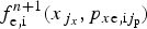$f_{{\rm e,i}}^{n{\rm + 1}} (x_{\,j_x},p_{x{\rm e,i}j_{\rm p}})$ is equal to $f_{{\rm e,i}}^n (x(t_n),p_{x{\rm e,i}}(t_n))$ , this latter value is calculated from the values of $f_{{\rm e,i}}^n $ at the grid points by a 2D interpolation using a tensor product of cubic B-splines (for details, see Shoucri et al., Reference Shoucri, Gerhauser and Finken2003; Shoucri, Reference Shoucri2008a , Reference Shoucri b ).

3. THE RELEVANT PARAMETERS

We first use the same parameters as in Shoucri and Afeyan (Reference Shoucri, Afeyan and Awrejcewicz2014), for the study we are presenting here for the SRBS and SKEENS processes. A characteristic parameter by which to refer to the amplitude of laser field is the normalized vector potential or quiver momentum $\left\vert {{\vec a}_ \bot} \right\vert = \left\vert {e{\vec A}_ \bot /M_{\rm e}c} \right\vert = a_0$ , where $\vec A_ \bot $ is the vector potential of the pump wave. For the linearly polarized wave, $a_0^2 = I{\rm \lambda} _0^2 /$ 1.368 × 10¹⁸. Here, I is the laser intensity in W/cm², and λ₀ the laser wavelength in microns. The pump wave frequency ω_0P of the injected laser beam is such that ${\rm \omega} _{{\rm 0P}}/{\rm \omega} _{{\rm pe}} = 1/\sqrt {n/n_{{\rm cr}}} $ , where n _cr is the critical density for the pump. In our calculation, n/n _cr = 0.0825, which corresponds to a pump frequency ω_0P = 3.481 (normalized to ω_pe). The amplitude of the vector potential of the pump is a _0P = 0.025. The seed backward pulse has a frequency ω_0B = 2.1657. The amplitude of the vector potential of the seed pulse for the Raman scattered backward wave is a _0B = a _0P = 0.025. The parameters of the backward KEEN wave will be discussed in Section 3.1.

The frequency and wavenumber (ω_0P, k _0P) of the pump wave are related by the relation ${\rm \omega} _{{\rm 0P}}^{\rm 2} = {\rm \omega} _{{\rm pe}}^{\rm 2} + k_{0{\rm P}}^2 c^2$ , or in normalized units ${\rm \omega} _{{\rm 0P}}^{\rm 2} = 1 + k_{{\rm 0P}}^{\rm 2} $ , from which k _0P = 3.3343. For the stimulated Raman scattering, or the coupling of a pump light wave to a daughter scattered light wave and an EPW, the values of the electron plasma wavenumber k _eB associated with SRBS mode, and k _eF associated with the SRFS mode are roots of the equation (Bers et al., Reference Bers, Shkarofsky and Shoucri2009):

(9) $$\eqalign{& \left[ {\left( {\displaystyle{{15\Omega} \over {4 - 6}}} \right)} \right]K^4 + ({\rm \mu} + 3\Omega - 3)K^2 - 2{\rm \mu} ^{1/2}\left[ {\Omega ^2 - 1 + \left( {\displaystyle{5 \over {2{\rm \mu}}}} \right)} \right]^{1/2}K \cr & \quad + 2\Omega - 1 - \left( {\displaystyle{5 \over {{\rm 2{\rm \mu}}}}} \right)(\Omega - 1) = 0}$$

with K = k _eλ_De, where λ_De is the Debye length. In our normalized units, the Debye length ${\rm \lambda} _{{\rm De}} = {\rm \upsilon} _{{\rm te}}/c = 0.04424\sqrt {T_{\rm e}} $ (λ_De normalized to c/ω_pe in our units, and T _e is in keV), and Ω = ω_0P (normalized to ω_pe). For the present problem we use hydrogen ions with M _i /M _e = 1836. We assume an electron temperature T _e = 2 keV, so λ_De = 0.06256. In Eq. (9), the parameter ${\rm \mu} = m_{\rm e}c^2/{\rm \kappa} T_{\rm e} = c^2/{\rm \upsilon} _{{\rm te}}^{\rm 2} = 1/(0.04424\sqrt {T_{\rm e}} )^2 = 255.8$ . The resulting roots are k _eBλ_De = 0.3377 for the plasma mode associated with the SRBS, and k _eFλ_De =0.0666 for the plasma mode associated with the SRFS. As discussed in Bers et al. (Reference Bers, Shkarofsky and Shoucri2009), for these parameters the SRBS plasma wave is damped, and the damping of the SRFS plasma wave is small. The heavily damped regime with k _eλ_De >0.29 is called the kinetic regime (Shoucri & Afeyan, Reference Shoucri, Afeyan and Awrejcewicz2014). We finally get k _eB = 0.3377/λ_De = 5.398 for the SRBS plasma wave, and k _eF = 0.0666/λ_De = 1.0645 for the SRFS plasma wave. The corresponding frequencies for the SRBS plasma wave and the SRFS plasma wave are solutions of the equation (Bers et al., Reference Bers, Shkarofsky and Shoucri2009):

(10) $${\rm \omega} ^2 \approx 1 + 3k^2{\rm \lambda} _{{\rm De}}^{\rm 2} /{\rm \omega} ^{\rm 2} + 15k^4{\rm \lambda} _{{\rm De}}^{\rm 4} /{\rm \omega} ^4 - 5/(2{\rm \mu} ).$$

We get from Eq. (10) for the SRBS wave ω_eB = 1.178, and for the SRFS plasma wave ω_eF = 1.0066. The selection rules give the following results for the forward scattered electromagnetic wave (ω_0F, k _0F) and the backward scattered electromagnetic wave (ω_0B, k _0B):

(11) $$\eqalign{& {\rm \omega} _{{\rm 0B}} = {\rm \omega} _{{\rm 0P}} - {\rm \omega} _{{\rm eB}} = 3.481 - 1.178 = 2.303; \cr & {\rm \omega} _{{\rm 0F}} = {\rm \omega} _{{\rm 0P}} - {\rm \omega} _{{\rm eF}} = 3.481 - 1.0066 = 2.4744; }$$

(12) $$\eqalign{& k_{{\rm 0B}} = k_{{\rm eB}} - k_{{\rm 0P}} = 5.398 - 3.3343 = 2.0637; \cr & k_{{\rm 0F}} = k_{{\rm 0P}} - k_{{\rm eF}} = 3.3343 - 1.0645 = 2.2698. }$$

Note the close values of (ω_0F, k _0F) with (ω_0B, k _0B). We verify that the results in Eqs. (11) and (12) obey the dispersion relation of the electromagnetic wave 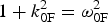$1 + k_{{\rm 0F}}^{\rm 2} = {\rm \omega} _{{\rm 0F}}^{\rm 2} $ (from which we get ω_0F = 2.48), and 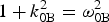$1 + k_{{\rm 0B}}^{\rm 2} = {\rm \omega} _{{\rm 0B}}^{\rm 2} $ (from which we get ω_0B = 2.293). These results are in very good agreement with the results calculated in Eq. (11). We note also the possibility of the anti-Stokes resonance ω_as = ω_0P + ω_eF = 3.481 + 1.006 = 4.487, k _as = k _0P + k _eF = 3.3343 + 1.0645 = 4.399. We calculate from the relation $1 + k_{{\rm as}}^{\rm 2} = {\rm \omega} _{{\rm as}}^{\rm 2} $ a value ω_as = 4.511, close to the value of 4.487 calculated from the selection rule. In addition, KEEN waves have been identified in (Afeyan et al. Reference Afeyan, Won, Savchenko, Johnston, Ghizzo, Bertrand, Hammel, Meyerhofer, Meyer-ter-Vehn and Azechi2004, Reference Afeyan, Casas, Crouseilles, Dodhy, Faou, Mehrenberger and Sonnendrucker2014, Mehrenberger et al. Reference Mehrenberger, Steiner, Maaradi, Crouseilles, Sonnendrücker and Afeyan2013, Shoucri and Afeyan Reference Shoucri, Afeyan and Awrejcewicz2014), which do not belong to the dispersion relations presented in Eqs. (9) and (10). The KEEN waves resulted from the scattering of the pump with the backward stimulated wave at (ω_0F, − k _0F), where (ω_0F, k _0F) are the frequency and wavenumber of the SFRS wave calculated in Eqs. (9) and (10). These will be discussed in more details in Section 3.1.

The ions were included in the calculation, but did not play any role in the physics except establishing a small self-consistent sheath at the edges. We use a fine resolution grid in phase space, with N = 30,000 grid points in space, and 512 grid points in momentum space for the electrons (extrema of the electron momentum are ± 0.5). We have initially a flat profile of a uniform plasma slab with the normalized density n _e = n _i = 1. This flat profile of the uniform plasma extends over a length L _p = 570.8c/ω_pe. On either side of the initial plasma slab the densities are smoothly brought down to zero through an initial parabolic profile of length L _edge = 8c/ω_pe. An extra vacuum region of length L _vac = 6.6c/ω_pe exists on each side of the slab, for a total length of the system of L = 600c/ω_pe. In our normalized units Δx = Δt = 0.02. We also have Δx/λ_De = 0.02/0.0626 ≈ 0.32.

3.1. Stimulated KEEN Wave Backscattering Pulse

The forward propagating linearly polarized wave is injected in the domain at the left boundary at x = 0 with $E^ + = 2E_{{\rm 0P}}\cos ({\rm \omega} _{{\rm 0P}}t)$ , E _0P = ω_0P a _0P, with a _0P = 0.025. The pump precursor reaches the right boundary at t = 600 (since in our normalized units x = t). As will be explained below, the KEEN wave is excited when a backward seed pulse is injected at the frequency of the forward scattered mode ω_0F = 2.474 (Shoucri & Afeyan, Reference Shoucri, Afeyan and Awrejcewicz2014). A seed pulse is injected at x = L in the backward direction in the form $E^ - = - 2E_{{\rm 0K}}P_{{\rm 0K}}(t)\cos {\rm \omega} _{{\rm 0F}}{\rm \tau} $ , where τ = t − t ₁. The temporal shape factor of the seed pulse is $P_{{\rm 0K}}(t) = \exp ( - 0.5(t - t_0)^2/{\rm \tau} _{\rm s}^{\rm 2} )$ , for t ₁ <t <t ₂. In this simulation we have τ_s = 15, t ₀ = 550, t ₂ = 600, t ₁ = 500, and E _0K = ω_0F a _0K, with a _0K = a _0P. In this way, the seed Gaussian pulse starts penetrating the domain from the right boundary at t = t ₁ = 500. When the pump precursor has reached the right boundary x = L = 600 at t = 600, the seed pulse injected at the right boundary of the domain in the backward direction has fully penetrated from the right boundary, and its peak has reached the point at x = 550 at the time t = 600.

We present first the results obtained for the forward propagating wave before the injection of the pulse. We show in Figure 1 the wavenumber spectra of the forward propagating signal E ⁺, the backward propagating signal E ⁻, and the longitudinal electric field. E ⁺ and E ⁻ are defined in Eq. (3). These spectra are calculated in the domain x = (20,164), at t = 800, well before the arrival of the seed pulse injected from the right boundary. The spectrum of E ⁺ shows the peak of the pump at k _0P = 3.3364, the peak of the forward scattered mode k _0F = 2.2626, very close to the value calculated in Eq. (12), and a small peak of the anti-Stokes mode at k _as = 4.41, very close to the theoretical value calculated at 4.399.

Fig. 1.

Wavenumber spectra of (clockwise) the incident wave E ⁺, the backward wave E ⁻, and the longitudinal electric field E _x , in the domain x = (20,164) at t = 800.

In free space, the forward propagating wave E ⁺ and the backward propagating wave E ⁻ are strictly decoupled. In a plasma, there is a very weak coupling between E ⁺ and E ⁻ due to the nonlinearity of the medium. So the wavenumber spectrum of the backward wave E ⁻ in the same domain x = (20,164) in Figure 1 shows the same peaks at 2.262, 3.336, and 4.41, but at a much lower level, even though the injected seed pulse at the right still did not reach the domain x = (20,164). Finally, we present also in Figure 1 the spectrum of the longitudinal electric field, which shows a broad peak at k _eF = 1.035 [theoretical value of 1.064 calculated from Eq. (9)]. We also see the peak at 6.6728.

Indeed, for the linearly polarized wave, we have a plasma mode appearing at the harmonic of the pump 2k _0P = 6.6728. This is due to the fact that if we have a linearly polarized wave: $\vec E = (0,E_y{\rm,} 0)$ , we can write in a linear analysis with $E_y = E_0\cos ({\rm \psi} )$ , ${\rm \psi} = (kx - {\rm \omega} t)$ , using Faraday's law:

(13) $$\displaystyle{{\partial \vec B} \over {\partial t}} = \left( {0,0, - \displaystyle{{\partial E_y} \over {\partial x}}} \right).$$

Then 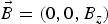$\vec B = (0,0,B_z)$ with $B_{\rm z} = B_0\cos ({\rm \psi} )$ , and B ₀ = E ₀ k/ω. From $\vec E_ \bot = - \partial \vec a_ \bot /\partial t$ from Eq. (2), and $\vec p_ \bot = \vec a_ \bot $ , we get $\vec p = (0,p_{\rm y},0)$ , with $p_{\rm y} = - p_0\sin ({\rm \psi} )$ , and p ₀ = E ₀/ω. The longitudinal Lorentz force is $p_yB_z = - (1/2)kp_0^2 \sin (2{\rm \psi} )$ . This drives a longitudinal response at the harmonic of the laser wave.

Figure 2 presents the frequency spectra of the waves. The frequency spectrum of the forward wave E ⁺ presented in Figure 2 shows the peak of the pump wave at ω_0P = 3.4898 (calculated at 3.481 in our theoretical results), the forward scattered frequency at ω_0F = 2.474, as calculated in Eq. (11), and the frequency of the anti-Stokes mode at ω_as = 4.51 as calculated in our theoretical results above. As explained above, there is a weak coupling of E ⁺ and E ⁻ which produces in the spectrum of E ⁻ the same frequencies as for E ⁺, but at a much lower level.

Fig. 2.

Frequency spectra of (clockwise) the incident wave E ⁺, the backward wave E ⁻, and the longitudinal electric field E _x , at the position x = 250, at time t = (260,328).

The frequency spectrum of the longitudinal electric field shows a peak of the plasma wave resonant with the forward scattering of the pump at ω_eF = 1.00 (theoretical value calculated at 1.0066). It also shows a peak at 6.96, which is the forced oscillation at the harmonic of the pump, as explained in Eq. (13). The small peaks at 5.963 and 7.976 seem to result from the resonance of the peak at 1.00 and the forced oscillation at 6.96, with 1.00 + 5.963 = 6.963 and 1.00 + 6.960 = 7.96.

As we mentioned above, there is a weak coupling of E ⁺ and E ⁻ which produces in the spectrum of E ⁻ a weak backward component at (ω_0F, − k _0F). This backward wave can couple with the forward propagating pump to produce a KEEN wave with the selection rule coupling k _0p = −k _0F + k _keen, from which k _keen = k _0P + k _0F = 3.334 + 2.27 = 5.60, as calculated in Shoucri and Afeyan (Reference Shoucri, Afeyan and Awrejcewicz2014). The frequency of this KEEN wave obey the coupling relation ω_0P = ω_0F + ω_keen, from which ω_keen = 3.481 − 2.474 = 1.007. The mode at 1.00 is indeed present in the spectrum of the longitudinal electric field in Figure 2 due to the forward Raman scattering, but the coupling with the KEEN wave at − k _0F is weak and shows no response at the wavenumber k _keen in the spectrum of the longitudinal electric field, because the mode at − k _0F in the spectrum of E ⁻ in Figure 1 is very weak. In the results presented in Shoucri and Afeyan (Reference Shoucri, Afeyan and Awrejcewicz2014), this mode was stimulated by a backward wave injected at − k _0F. This mode can also be stimulated in the present simulation by the pulse we injected as described above at the right boundary with a frequency ω_0F, propagating in the backward direction. We present in Figure 3 the electron density profile and the longitudinal electric field profile at t = 840, when the pulse injected at the right boundary with a frequency ω_0F and traveling to the left has reached a point close to x = 300.

Fig. 3.

Plot of the electron density profile (left frame) and the longitudinal electric field E _x (right frame) at time t = 840.

We present in Figure 4 the spectra of the longitudinal electric field at the arrival of this pulse (ω_0F, − k _0F) in the domain x = (20,348), at t = 800 and at t = 840. We can verify from Figure 3 that at this time the signal has just penetrated from the right into the domain x = (20,348). In Figure 4 at t = 800 (left panel) we see indeed the growing mode (compare with Fig. 1) with a broad peak at k _keen = 5.58, very close to the theoretical value of 5.60 calculated in the previous paragraph. So the wavenumber response of the system to the backward pulse injected at the right boundary at the frequency ω_0F is indeed a KEEN wave at k _keen = 5.58. The right panel in Figure 4 gives the wavenumber spectrum at t = 840 in the same domain, showing again the continued growth of the mode at k _keen = 5.58, which is now developing a harmonic structure.

Fig. 4.

Wavenumber spectra of the longitudinal electric field E _x in the domain x = (20,348), at time t = 800 (left frame), and t = 840 (right frame).

We present in Figure 5 the wavenumber spectra of the forward wave E ⁺ and backward wave E ⁻ at t = 840. The presence of the backward mode k _0F at 2.262 in the spectrum of E ⁻ is now growing to become dominant, showing a broad peak. So the system is responding to the arrival of the seed pulse injected with ω_0F = 2.474 from the right boundary in the backward direction with a growing mode at k _0F = 2.262 in the spectrum of E ⁻ as it should. The forward wave E ⁺ at k _0P = 3.336 can now couple with the backward wave of the pulse at − k _0F = −2.262 with k _0p = −k _0F + k _keen to produce the KEEN wave with k _keen = k _0P + k _0F = 3.334 + 2.262 = 5.596, which we observe at 5.58 in Figure 4. The wavenumber at k _eF = 1.074 in Figure 4 is the result of the forward scattering k _0P = k _0F + k _eF, calculated at k _eF = 1.0645 in our theoretical results in Eq. (12).

Fig. 5.

Wavenumber spectra of the forward pump wave E ⁺ (left frame) and the backward wave E ⁻ (right frame), in the domain x = (20,348) at t = 840.

The frequency spectra are presented in Figure 6. These spectra are calculated from the registered signals at x = 250 at the arrival of the pulse, from the time t = 623 to t = 990. We see in the spectrum of the forward wave E ⁺ the presence of the pump frequency at ω_0P = 3.4898, of the forward scattered mode at ω_0F = 2.474, and the anti-Stokes mode ω_as = 4.49. The frequency spectrum of the backward wave E ⁻ shows the peak at 3.4898, and a broad peak at 2.454 (slightly shifted from the value of 2.474 observed in Fig. 2). The coupling of forward wave E ⁺ at 3.4898 and the backward wave at 2.454 according to the selection rule ω_0P = ω_0F + ω_keen produces the frequency 3.4898 − 2.454 = 1.036, very close to the value of 1.054 in the broad peak appearing the spectrum of the longitudinal electric field in Figure 6. We note also in the spectrum of the longitudinal electric field in Figure 6 the values of 1.00, and 6.96 previously identified in Figure 2. Different small peaks are also appearing. It is important at this stage to insist on the transient nature of the modes we are studying.

Fig. 6.

Frequency spectra of (clockwise) the incident wave E ⁺, the backward wave E ⁻, and the longitudinal electric field E _x , at the position x = 250, at time t = (623,990).

We present in Figure 7 a phase-space plot at t = 840 showing the growth of the KEEN wave at the arrival of the backward pulse around x = 320. The phase velocity of the KEEN wave is υ_keen = 1.054/5.58 = 0.19, corresponding to $p_{{\rm keen}} = {\rm \upsilon} _{{\rm keen}}/\sqrt {1 - {\rm \upsilon} _{{\rm keen}}^{\rm 2}} = 0.1935$ , which is essentially the value we see at the center of the vortex at the right in Figure 7.

Fig. 7.

Phase-space plot of the electron distribution function in the domain x = (320,360), at time t = 840 at the arrival of the KEEN wave around x = 320.

After the analysis we have presented of the initial KEEN response of the system to the pulse injected at the right boundary at the frequency ω_0F = 2.474, we now look to the final evolution of the system. We present in Figure 8 a plot at t = 1000 and 1116 of the incident pump (full curve) and the pulse (dashed curve). The pulse injected at the right boundary in the backward direction as explained before has now traveled to the left. The incident pump with constant amplitude at the left boundary goes through a phase of partial depletion after the crossing of the pulse coming from the right. The growth of the pulse is small in the present case, and does not show a significant contraction. Its initial peak value of E ⁻ when injected was 2ω_0F a _0K = 0.124, and is reaching toward the end (see the dashed curve in Fig. 8) a value about 0.4, more than three times higher than the initially injected amplitude, and about twice bigger than the amplitude of the injected pump E ⁺ field at the left.

Fig. 8.

The evolution of the incident forward pump wave E ⁺ (full curve), and the backward seed pulse E ⁻ (dashed curve) at t = 1000 (left frame) and t = 1116 (right frame).

Figure 9 presents the plot of the electron density and the longitudinal electric field at t = 1000. It shows the profile maintaining a coherent structure.

Fig. 9.

Plot of the electron density profile (left frame) and the longitudinal electric field E _x (right frame) at time t = 1000.

Figure 10 presents the wavenumber spectra of the pump E ⁺, the backward wave E ⁻, and the longitudinal electric field, taken in x = (180,344) at t = 1000, at the edge where from Figure 9 the spatial structure appears coherent. We see the now dominant peak of the backward wave E ⁻ at 2.186. The peak of the pump E ⁺ appears at k _0p = 3.336. We still have a forward scattering, and the forward scattered mode appears now at k _0F = 2.262, previously obtained in Figures 1 and 5. The plasma mode k _eF resulting from the forward scattering k _0p = k_0F + k _eF is present in the spectrum of the longitudinal electric field at k _eF = 3.336 − 2.262 = 1.074. The wavenumber of the KEEN wave is now determined by the pump interacting with the backward dominant peak at 2.186, at k _keen = 3.336 + 2.186 = 5.522, clearly dominant in the spectrum of the longitudinal electric field in Figure 10 (slightly shifted from the value of 5.58 initially calculated in Fig. 4). We see also the harmonic of this peak appearing in the wavenumber spectrum of the longitudinal electric field in Figure 10. We note in the spectrum of E ⁺ the peak of the anti-Stoke at 4.37. We now also see the small peak of the backward Raman scattered mode appearing at k _0B = 2.07 in the spectrum of E ⁻ [calculated at 2.0637 in Eq. (12)]. The now dominant backward mode at 2.186 in the spectrum of E ⁻ can also directly interact with the plasma KEEN mode, generating the mode at −7.67, with the relation − 2.186 = −7.67 + k _keen, from which we get k _keen = 5.484 (appearing at 5.522 in the spectrum in Fig. 10). And in the spectrum of E ⁺ the pump at 3.336 can also directly interact with the plasma KEEN mode, generating the mode at 8.858, with the relation 8.858 = 3.336 + k _keen, from which we get k _keen = 5.522, appearing in the spectrum in Figure 10. Also in the spectrum of E ⁺ the mode 7.7 couples with the mode at 2.186 through the relation 7.7 = 2.186 + k _keen, from which k _keen = 5.514, very close to the value of 5.52 in Figure 10.

Fig. 10.

Wavenumber spectra of (clockwise) the incident wave E ⁺, the backward wave E ⁻, and the longitudinal electric field E _x , in the domain x = (180,344) at t = 1000.

The frequency spectra registered at time t = (920,1084), during the passage of the homogeneous front of the signal at the point x = 250, are presented in Figure 11. The spectrum of the pump E ⁺ shows the frequency ω_0P = 3.4898, the backward wave E ⁻ is now dominated by a broad peak at the frequency 2.377 (evolving by a small shift from the value of 2.474 in Fig. 2 and 2.454 in Fig. 6). The relation 3.4898 = 2.377 + ω_keen gives ω_keen = 1.11, close to the broad peak at 1.073 in the frequency spectrum of the longitudinal electric field in Figure 11. The frequency of the anti-Stoke is at 4.487.

Fig. 11.

Frequency spectra of (clockwise) the incident wave E ⁺, the backward wave E ⁻, and the longitudinal electric field E _x , at the position x = 250, at time t = (920,1084).

We present in Figure 12 the plots of the electron density and the longitudinal electric field at the end of the simulation at t = 1116. The front edge is still maintaining coherence, and hence still maintaining the growth of the pulse, while the remaining profile is becoming chaotic due to the fusion of vortices in the phase space. The vortices in the front edge are presented in Figure 13, in x = (20,60) and x = (60,100). We present in Figure 14 the distribution function spatially averaged over a wavelength at t = 1116, taken from the results in Figure 13, at the position x = 60 and 100.

Fig. 12.

Plot of the electron density profile (left frame) and the longitudinal electric field E _x (right frame) at time t = 1116.

Fig. 13.

Phase-space plot of the electron distribution function in the domain x = (20,100), showing the vortices in the front edge at time t = 1116.

Fig. 14.

The distribution function spatially averaged over a wavelength around the positions (a) x = 60 and (b) x = 100, at time t = 1116.

Figure 15 presents the wavenumber spectra of the pump E ⁺, the backward wave E ⁻, and the longitudinal electric field, taken at the front edge in x = (20,102) at t = 1116, at the end of the simulation. They are close to what is presented in Figure 10. We see the now dominant peak of the backward wave E ⁻ at 2.186. The peak of the pump E ⁺ appears at k _0p = 3.374. We still have a forward scattering, and the forward scattered mode appears now at k _0F = 2.3, slightly shifted from the value of 2.262 obtained in Figures 1 and 5, since the plasma mode k _eF resulting from the forward scattering k _0P = k _0F + k _eF is present in the spectrum of the longitudinal electric field at k _eF = 3.374 − 2.3 = 1.074. The wavenumber of the KEEN wave is now determined by the pump interacting with the backward dominant peak at 2.186, at k _keen = 3.374 + 2.186 = 5.56, very close to the peak calculated at 5.522 in Figure 15 (slightly shifted from the value of 5.58 in Fig. 4). We see also the harmonic of this peak appearing in the wavenumber spectrum of the longitudinal electric field in Figure 15. We note in the spectrum of E ⁺ the peak of the anti-Stoke at 4.41. We now see also a small peak of the backward Raman scattered mode appearing at k _0B = 2.07 in the spectrum of E ⁻ [calculated at 2.0637 in Eq. (12)]. The now dominant backward mode at 2.186 can also directly interact with the plasma KEEN mode, generating in the backward direction the mode at 7.746 in the spectrum of E ⁻, with the relation −2.186 = −7.746 + k _keen, from which we get k _keen = 5.56 (appearing at 5.522 in the spectrum).

Fig. 15.

Wavenumber spectra of (clockwise) the incident wave E ⁺, the backward wave E ⁻, and the longitudinal electric field E _x , in the domain x = (20,102) at t = 1116.

The frequency spectra registered in t = (920,1084), during the passage of the homogeneous front of the signal at the point x = 250, are presented in Figure 11.

3.2. Raman Backscattered Wave Pulse

We use the same parameters as in Section 3.1. However, the pulse injected at the right boundary has a frequency ω_0B = 2.30, which is the frequency of the backward scattered Raman wave, which is calculated in Eq. (11). The pump and all other parameters remain the same. The first part of the simulation, when the pump is propagating in the forward direction, before the injection of the pulse, is therefore identical to what has been presented in Figures 1 and 2 for the excitation of the Raman forward scattered wave. After the injection of the pulse from the right boundary in the backward direction in the same way as described above for the KEEN wave, the propagating pulse will interact with the pump and start growing. Figure 16 shows the density plot and the electric field plot at t = 840, to be compared with Figure 3. There is a difference in the spatial topology of these plots, compared with the corresponding ones in Figure 3.

Fig. 16.

Plot of the electron density profile (left frame) and the longitudinal electric field E _x (right frame) at time t = 840.

Figure 17 shows the wavenumber spectra of the longitudinal electric field at t = 800 (left panel) and t = 840 (right panel), at the time the pulse injected from the right boundary is arriving in the domain x = (20,348), to be compared with Figure 4. We see in the left panel the system responding with the appearance of the plasma wave at k _eB = 5.39 due to the backward Raman scattering in agreement with Eq. (12), in addition with the plasma wave at k _eF = 1.074 due to the forward Raman scattering [calculated at 1.0645 in Eq. (12)], and the mode at the pump harmonic 2k _0P = 6.672, as explained in the previous section at Eq. (13).

Fig. 17.

Wavenumber spectra of the longitudinal electric field E _x in the domain x = (20,348), at time t = 800 (left frame), and t = 840 (right frame).

The right panel in Figure 17 shows the spectrum of the electric field at t = 840. The plasma mode is slightly shifted at k _eB = 5.426, and has developed harmonics at 10.872 and 16.413. The wavenumber spectra of the forward pump wave E ⁺ and the backward wave E ⁻ at t = 840 are presented in Figure 18. We see in addition to what is presented in Figure 5, the appearance of the backward pulse with wavenumber at 2.07 [calculated at 2.063 in Eq. (12)], which is now the dominant mode in the spectrum of the backward wave E ⁻. To be compared with Figure 5.

Fig. 18.

Wavenumber spectra of the forward pump wave E ⁺ (left frame) and the backward wave E ⁻ (right frame), in the domain x = (20,348) at t = 840.

The frequency spectra of the growing waves at the arrival of the pulse are calculated from the recorded signal at x = 250 from t ₁ = 623 to t ₂ = 951. In Figure 19, we present the frequency spectra of the forward pump wave E ⁺, the backward pulse wave E ⁻ and the longitudinal electric field. We see in the spectrum of E ⁻ the dominant backward pulse wave at the frequency 2.32 [calculated at 2.30 in Eq. (11)]. This peak appears in the spectrum of E ⁺, together with the frequency of the forward scattered mode at 2.474, the pump frequency at 3.4898, and the anti-Stoke frequency at 4.48. The frequency spectrum of the evolving longitudinal wave in Figure 19 show a broad peak at 1.16, and the frequency at the harmonic of the pump frequency 2ω_0P = 6.96, as explained in Eq. (13). Figure 19 is to be compared with Figure 6.

Fig. 19.

Frequency spectra of (clockwise) the incident wave E ⁺, the backward wave E ⁻, and the longitudinal electric field E _x , at the position x = 250, at time t = (623,951).

We present in Figure 20 a phase-space plot at t = 840 showing the growth of the backward Raman scattered wave at the arrival of the backward pulse around x = 320, showing a much more rapid growth compared with Figure 7.

Fig. 20.

Phase-space plot of the electron distribution function in the domain x = (320,360), at time t = 840 at the arrival of the backward Raman scattered wave around x = 320.

The density and longitudinal electric field plots at t = 1000 are shown in Figure 21. They are still maintaining the coherent structure. However, the morphology of the modulations in Figure 21 are sharply different from what we observed in Figure 9. Figure 22 presents the plots of the forward pump wave E ⁺ (full curve) and the backward pulse wave E ⁻ (dashed curve) at t = 1000 (left panel) and t = 1116 (right panel). The growth of the pulse is more important to what is presented in Figure 8.

Fig. 21.

Plot of the electron density profile (left frame) and the longitudinal electric field E _x (right frame) at time t = 1000.

Fig. 22.

The evolution of the incident forward pump wave E ⁺ (full curve), and the backward seed pulse E ⁻ (dashed curve) at t = 1000 (left frame) and t = 1116 (right frame).

We present now the final state of the system. Figure 23 presents the plot of the density and the longitudinal electric field at t = 1116. It shows the front maintaining a coherent structure, while to the right the fusion of the excited vortices is creating a chaotic structure. We look in Figure 24 into the phase space of the coherent structure at the left in Figure 23, from x = 20 to 100. It shows a dominant vortex structure. Figure 24 shows the growth of the vortices much more rapid than what is presented in Figure 13.

Fig. 23.

Plot of the electron density profile (left frame) and the longitudinal electric field E _x (right frame) at time t = 1116.

Fig. 24.

Phase-space plot of the electron distribution function in the domain x = (20,100), showing the vortices in the front edge at time t = 1116.

Figure 25 gives at t = 1116 the distribution function at x = 60 (left frame) and at x = 100 (right frame), spatially averaged over a wavelength. At x = 60, Figure 24 indicates we still are at in a transition showing growing vortices. At x = 100, the vortices seem to have reach a steady state. We look for the spatially averaged distribution function at x = 100. It shows a local minimum around p _xe = 0.2, around the phase of the saturated wave. By looking to the spectra of the system close to the left boundary at the end of the simulation in the domain x = (20,184) in Figures 26 and 27 below, we get for the frequency of the longitudinal electric field the value 1.112 in Figure 27, and wavenumber of 5.484 in Figure 26, we deduce a phase velocity υ_phase ≈ 0.20, and a momentum $p_{{\rm phase}} = {\rm \upsilon} _{{\rm phase}}/\sqrt {1 - {\rm \upsilon} _{{\rm phase}}^{\rm 2}} $ , from which p _phase = 0.204, very close to the local minimum we see in the plot of the distribution function on the right side of Figure 25.

Fig. 25.

The distribution function spatially averaged over a wavelength around the positions x = 60 (left frame), and x = 100 (right frame), at time t = 1116.

Fig. 26.

Wavenumber spectra of (clockwise) the incident wave E ⁺, the backward wave E ⁻, and the longitudinal electric field E _x , in the domain x = (20,184) at t = 1116.

Fig. 27.

Frequency spectra of (clockwise) the incident wave E ⁺, the backward wave E ⁻, and the longitudinal electric field E _x , at the position x = 250, at time t = (920,1084).

Figure 26 presents the wavenumber spectra of the pump E ⁺, the backward wave E ⁻, and the longitudinal electric field. The frequency spectra in Figure 27 are obtained by taking the spectra of E ⁺, E ⁻ and the longitudinal electric field, registered at x = 250 during the passage of the front of the pulse, from t ₁ = 920 to t ₂ = 1084. The spectrum of E ⁻ has now the dominant modes, with a broad spectrum for the peak value. In Figure 26, the peak wavenumbers for E ⁻ extend from 2.109 to 2.186. The peak at 2.186 is the same as the one we got in Figure 15, and the peak at 2.109 is close to the value of 2.063 calculated in Eq. (12) for the backscattered Raman wave. In Figure 27, the peak frequencies for E ⁻ extend from 2.34 to 2.37. We also see the anti-Stokes at 4.52. The peak at 2.37 is the same as the one we see in Figure 16, and the peak at 2.34 is close to the frequency of 2.30 calculated in Eq. (11) for the frequency of the backscattered Raman wave. So in addition to the peaks we got in the study of the KEEN wave in Section 3.1, we have in the present case a clear coupling with the backscattered Raman wave. We are far from the picture of a single peak mode dominating the final spectrum. The dominant E ⁻ mode now dominates the mode coupling process. The wavenumbers of 2.109 and 2.186 are also appearing in the spectrum of E ⁺. The pump has shifted slightly to 3.298. We also see the anti-Stokes wavenumber at 4.41. We see in Figure 26, in the spectrum of the longitudinal electric field, the wavenumber coupling 3.298 ≈ −2.186 + k _eB leads to k _eB ≈ 5.484. We also see in Figure 26 the harmonics at 10.968, 16.59, 21.86, and 27.42. The peak in E ⁻ at the wavenumber 2.186 would also interact with the peak at 5.485 of the longitudinal electric field to −2.186 = −k + 5.484, from which the mode at k = 7.67, which appears in the spectrum of E ⁻ in Figure 26. It also appears in the forward direction in the spectrum of E ⁺ 7.67 = 2.186 + 5.484. Also in the spectrum of E ⁺ the peak at 3.298 and the peak at 8.78 (not indicated in the figure) can couple 8.78 = 3.298 + 5.484.

We see in Figure 27 in the frequency spectrum of E ⁻ the dominant backward pulse dominated by the peaks at 2.34–2.37 [calculated at 2.30 in Eq. (11)]. This peak appears in the spectrum of E ⁺. We also see the anti-Stokes frequency at 4.52. The plasma wave associated with the forward scattered mode now appears at the frequency 3.4898 ≈ 2.34 + ω_eF (and also for the backward scattered mode and the KEEN wave), from which ω_eF ≈ 1.15, very close to the broad peak at 1.112 which appears in the frequency spectrum of longitudinal electric field (together with harmonics).

4. ANOTHER EXAMPLE OF SEED PULSE AMPLIFICATION

We now analyze the results of a simulation using parameters similar to those presented in Mourou et al. (Reference Mourou, Fisch, Malkin, Toroker, Khazanov, Sergeev, Tajima and LeGarrec2012). In the present calculation, n/n _cr = 0.1, which corresponds in this case to the pump wave frequency of the injected laser beam ${\rm \omega} _{{\rm 0P}} = 1/ \sqrt {n/n_{{\rm cr}}} = 3.481$ (normalized to the plasma frequency ω_pe, n _cr is the critical density for the pump). For the linearly polarized wave $a_0^2 = I{\rm \lambda} _0^2 /$ 1.368 × 10¹⁸, I is the laser intensity in W/cm², and λ₀ the laser wavelength in microns In the present calculation the wavelength of the pump is λ_0P = 1.05 μm, and the laser intensity is I _0P = 2 × 10¹⁵ W/cm², which corresponds to an amplitude of the vector potential of the pump a _0P = 0.04. The seed Raman backscattered pulse has a frequency ω_0B = 2.1657 and a wavelength λ_0B = 1.541 μm. The laser intensity is I _0B = 1 × 10¹⁴ W/cm², which corresponds to an amplitude of the vector potential of the seed pulse is a _0B = 0.01318.

The frequency and wavenumber (ω_0P, k _0P) of the pump wave are related in normalized units by the relation ${\rm \omega} _{{\rm 0P}}^{\rm 2} = 1 + k_{{\rm 0P}}^{\rm 2} $ , from which k _0P = 3.0185. For the stimulated Raman scattering, or the coupling of a pump light wave to a daughter scattered light wave and an EPW, the values of the electron plasma wavenumber k _eB associated with the stimulated Raman backscattered mode SRBS, and k _eF associated with the stimulated Raman forward scattered mode SRFS are roots of Eq. (9). For the present problem we also have hydrogen ions with M _i /M _e = 1836. We assume an electron temperature T _e = 0.2 keV. In Eq. (9), the parameter ${\rm \mu} = m_{\rm e}c^2/{\rm \kappa} T_{\rm e} = c^2/{\rm \upsilon} _{{\rm te}}^{\rm 2} = $ $1/(0.04424\sqrt {T_{\rm e}} )^2 = 2555$ . The resulting roots of Eq. (9) are k _eBλ_De = 0.09774 for the plasma mode associated with the SRBS, and k _eFλ_De = 0.0214 for the plasma mode associated with the SRFS. In our normalized units the Debye length ${\rm \lambda} _{{\rm De}} = {\rm \upsilon} _{{\rm te}}/c = 0.04424\sqrt {T_{\rm e}} $ (T _e is in keV), so λ_De = 0.0198 for T _e = 0.2 keV. We finally get k _eB = 0.09774/λ_De = 4.94 for the SRBS plasma wave, and k _eF = 0.0214/λ_De = 1.0816 for the SRFS plasma wave. The corresponding frequencies for the SRBS plasma wave and the SRFS plasma wave are solutions of Eq. (10). We get for the SRBS wave ω_eB = 1.0134, and for the SRFS plasma wave ω_eF = 1.000. The selection rules give the following results for the forward scattered electromagnetic wave (ω_0F, k _0F) and the backward scattered electromagnetic wave (ω_0B, k _0B):

(14) $$\eqalign{& {\rm \omega} _{{\rm 0B}} = {\rm \omega} _{{\rm 0P}} - {\rm \omega} _{{\rm eB}} = 3.18 - 1.0134 = 2.166; \cr & {\rm \omega} _{{\rm 0F}} = {\rm \omega} _{{\rm 0P}} - {\rm \omega} _{{\rm eF}} = 3.18 - 1.000 = 2.18,}$$

(15) $$\eqalign{& k_{{\rm 0B}} = k_{{\rm eB}} - k_{{\rm 0P}} = 4.94 - 3.0185 = 1.9215; \cr & k_{{\rm 0F}} = k_{{\rm 0P}} - k_{{\rm eF}} = 3.0185 - 1.081 = 1.9375.}$$

Note the close values of (ω_0F, k _0F) with (ω_0B, k _0B). We verify that the results in Eqs. (14) and (15) obey the dispersion relation of the electromagnetic wave 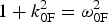$1 + k_{{\rm 0F}}^{\rm 2} = {\rm \omega} _{{\rm 0F}}^{\rm 2} $ , (from which we get ω_0F = 2.18), and $1 + k_{{\rm 0B}}^{\rm 2} = {\rm \omega} _{{\rm 0B}}^{\rm 2} $ (from which we get ω_0B = 2.166). These results are in very good agreement with the results in Eq. (14). We note also the possibility of the anti-Stokes resonance according to the selection rules ω_as = ω_0P + ω_eF = 3.18 + 1.00 = 4.18, k _as = k _0P + k _eF = 3.0185 + 1.081 = 4.099. We calculate from the relation $1 + k_{{\rm as}}^{\rm 2} = {\rm \omega} _{{\rm as}}^{\rm 2} $ a value ω_as = 4.219, close to the value of 4.18 calculated from the selection rule. As discussed in Section 3, KEEN waves have been identified in Shoucri and Afeyan (Reference Shoucri, Afeyan and Awrejcewicz2014), which do not belong to the dispersion relations presented in Eqs. (9) and (10) and resulted from the backscattering of the pump with the backward stimulated wave at (ω_0F, − k _0F). This results in a coupling very close to the coupling of the backscattered Raman wave (ω_0B, − k _0B), since as we previously noted in Eqs. (14) and (15), these values are very close.

The ions were included in the calculation but did not play any role in the physics except establishing a small self-consistent sheath at the edges. We use a fine resolution grid in phase space, with N = 30,000 grid points in space, and 800 grid points in momentum space for the electrons (extrema of the electron momentum are ± 1.2). We use the same plasma profile as in Section 3, with the same total length of the system of L = 600c/ω_pe. In our normalized units Δx = Δt = 0.02. We also have Δx/λ_De ≈ 1.01.

The forward propagating linearly polarized wave is injected in the domain at the left boundary at x = 0 with $E^ + = $ $2E_{{\rm 0P}}\cos ({\rm \omega} _{{\rm 0P}}t)$ , E _0P = ω_0P a _0P, with a _0P = 0.04. The pump precursor reaches the right boundary at t = 600 (since in our normalized units x = t). A seed pulse is injected at x = L in the backward direction in the form $E^ - = - 2E_{{\rm 0B}}P_{{\rm 0B}}(t) \cos {\rm \omega} _{{\rm 0B}}{\rm \tau}, $ where ω_0B = 2.166 and τ = t − t ₁. The temporal shape factor of the seed pulse is $P_{{\rm 0B}}(t)$ similar to the expression in Section 3, with τ_s = 6.2, t ₂ = 600, t ₀ = 580, t ₁ = 560, t ₁ < t < t ₂. E _0B = ω_0B a _0B with a _0B = 0.01318. In this way, the seed Gaussian pulse starts penetrating the domain from the right boundary at t = t ₁ = 560. When the pump precursor has reached the right boundary x = L = 600 at t = 600, the seed pulse has fully penetrated from the right boundary, and its peak has reached the point at x = 580 at the time t = 600.

For the parameters used in this simulation, the SRFS plasma mode with k _eFλ_De = 0.0214 is very weakly damped (Bers et al., Reference Bers, Shkarofsky and Shoucri2009). No seed or initial perturbation is added to stimulate the more damped SRBS mode with k _eBλ_De = 0.09774. We present in Figure 28 the evolution of the incident pump E ⁺ wave (full curve) and the backward seed pulse E ⁻ (dashed curve) at: (a) t = 820, (b) t = 920, (c) t = 1160, (d) t = 1220. The growth and contraction of the seed pulse (dashed curves), propagating toward the left, is obvious, and also the detachment of the front of the growing seed pulse. The constant amplitude full curve at the left is for the constant amplitude incident pump. Once the seed is reaching the same amplitude as the pump, we enter the regime of pump depletion. The smaller peaks we see behind the front pulse of the growing seed are due to the fact that when the pump depletes, the seed pulse can lose energy again for the pump, which results in the oscillations in the tail of the seed we observe (i.e. the amplified seed beats with the plasma wave to regenerate the pump, which results in the depletion of the seed). Also, the exchange with the anti-Stokes resonance can play a similar role in this oscillation.

Fig. 28.

Evolution of the incident pump E ⁺ wave (full curve) and the backward seed pulse E ⁻ (dashed curve) at: (a) t = 820, (b) t = 920, (c) t = 1160, (d) t = 1220; τ_s = 6.2 and a _0P = 0.04.

We present in Figure 29 a plot of the electron density at t = 1160 and 1220, corresponding to Figures 28c and 28d, and in Figure 30 the electron density in the region of the front edge in $x \in (15,65)$ at t = 1220. We observe regular oscillations in the front edge in $x \in (15,65)$ . The wavelength associated with these regular oscillations is the wavelength of the growing seed pulse, which is λ_eB = 2π/k _eB =1.27, which is also very close to the value of λ_eF as we have mentioned from the results of Eq. (15). We shall see below that this corresponds to coherent vortical structures in phase-space, while the part of the density plots in Figure 29, which shows a rather noisy density profile to the right, corresponds to a region in phase space where vortices were actively merging.

Fig. 29.

Plot of the electron density profile at t = 1160 and 1220; τ_s = 6.2 and a _0P = 0.04

Fig. 30.

Plot of the electron density in the region of the front edge in $x \in (15,65)$ at t = 1220.

This is also shown in Figure 31, where we present in the phase-space the contour plots of the electron distribution function in $x \in (15,65)$ , and in $x \in (65,115)$ at t = 1220. In $x \in (15,65),$ we observe a more coherent vortices structure (corresponding to the profile we see in Fig. 30), while in $x \in (65,115)$ we see the vortices at the right of the figure who are coalescing together, leading to the somewhat noisy structure we see at the right the density plots in Figure 29.

Fig. 31.

Phase-space plot of the electron distribution function in $x \in (15,65)$ and in $x \in (65,115)$ , at t = 1220.

We present in Figure 32 the wavenumber spectra of the incident wave E ⁺, the backward wave E ⁻ and the longitudinal electric field in the domain $x \in (140,468)$ at the time t = 640, well before the backward injected seed reaches this part of the domain. The only excited waves in this case are due to the forward propagating pump E ⁺. We recognize the peak of the pump E ⁺ at k _0P = 3.01 [calculated at 3.0184 in our theoretical calculations in Eq. (15)]. The pump is exciting a weakly damped, forward propagating wave with wavenumber k _0F = 1.936, in agreement with our theoretical results in Eq. (15). We have also a very small peak for the anti-Stokes wavenumber at k _as = 4.1034 (calculated at 4.099 in our theoretical calculations). Since the plasma is a nonlinear medium, the same modes are appearing in the spectrum of the backward wave E ⁻ at much lower amplitude, as previously explained. The wavenumber spectrum of the excited longitudinal electric field show the wavenumber of the resonant plasma mode for the forward wave at k _eF = 1.0738 (calculated at 1.081 in our theoretical calculations). The values of k _0B and k _0F in Eq. (15) are very close. The pump at 3.0104 in the spectrum of E ⁺ in Figure 32 can couple with the mode at 1.9366 in the spectrum of E ⁻ to produce the plasma mode at 3.0104 = −1.9366 + k _keen, or k _keen = 4.977, very close to the calculated plasma wave k _eB = 4.94 associated with the backscattered Raman wave (the spectrum of the longitudinal electric field shows a peak at 4.966 in Fig. 32). So even though the seed pulse is still far away, there is a small plasma mode at 4.966 excited well before the arrival of the seed pulse, associated with the backward resonance due to the coupling of the pump at k _0P = 3.0104 in E ⁺ (which is exciting the forward scattered mode at k _0F = 1.936), with the backward mode appearing at 1.936 in the spectrum of E ⁻ in Figure 31. So the pump is exciting the plasma mode around 4.96 through two backward resonances. A backward resonance with the KEEN wave 3.0104 = −1.936 + 4.977, and the resonance with the seed pulse, which still did not take place in the spectra in Figure 32 at t = 600. Finally for the linearly polarized wave, we have a plasma mode appearing in the spectrum of the longitudinal wave at the harmonic of the pump 2k _0p = 6.04 (calculated at 6.036 in our theoretical results), as explained in Eq. (13). The forced oscillations at the wavenumber 6.04 further stimulate the mode at 4.966, by coupling with the plasma wave at 1.0738, through the selection rule 6.04 = 4.966. + 1.0738. Also a longitudinal mode appears at 7.1138 through the coupling 7.1138 = 6.040 + 1.0738.

Fig. 32.

Wavenumber spectra of (clockwise) the incident wave E ⁺, the backward wave E ⁻ and the longitudinal electric field in the domain $x \in (140,468)$ at time t = 640.

Figure 33 presents the frequency spectra of the pump wave E ⁺, the backward wave E ⁻ and the longitudinal electric field, from the data recorded at the position x = 150 between t ₁ = 492 and t ₂ = 819, before the arrival of the backward propagating pulse. The spectrum of E ⁺ in Figure 33 shows the pump frequency at 3.183 [calculated 3.18 in Eq. (14)], the forward scattered mode at 2.183 [calculated at 2.18 in Eq. (14)]. The anti-Stokes mode is at 4.18 (calculated at 4.18). These same modes appear in the spectrum of E ⁻ in Figure 33 as previously explained. We see a mode of frequency 1.00 in the frequency spectrum of the longitudinal electric field excited though the forward coupling 3.183 = 2.183 + 1.00. We also see the mode at the harmonic of the pump 2ω_0p = 6.366 as explained in Eq. (13). And the coupling of the pump with the wave at (ω_0F, − k _0F) produces a KEEN wave as explained in Section 3, with frequency 3.183 = 2.183 + ω_keen, from which ω_keen = 1.00. Note the mode at 5.369 which can be excited through the forced oscillation 1.00 + 5.369 = 6.369, very close to the forced oscillation at 6.366. We also note in Figure 33 the possible further forced resonance 3.183 + 2.183 = 5.366, very close to the mode at 5.369.

Fig. 33.

Frequency spectra of (clockwise) the incident wave E ⁺, the backward wave E ⁻, and the longitudinal electric field E _x , at the position x = 150, at time t = (192,819).

We look again in Figure 34 to the wavenumber spectra in the same domain $x \in (140,468)$ , the same domain as in Figure 32, but at the time t = 740, when the backward pulse has entered the domain $x \in (140,468)$ . The spectrum of E ⁺ is essentially the same as in Figure 32, however the mode at 1.936 is more stimulated. The spectrum of E ⁻ in Figure 34 however shows the effect of the arrival of the pulse. There is a broad peak. We are still in a transient phase, and this broad peak is due to the presence of the mode at 1.936 which results from the forward coupling of the pump 3.010 = 1.936 + 1.074 (the mode in the spectrum of the longitudinal electric field appears at 1.073), the KEEN wave coupling 3.010 = −1.936 + k _keen, from which k _keen = 4.946, which we see in the spectrum of the longitudinal electric field. Finally, the frequency of the arriving pulse from Eq. (14) is at ω_0B = 2.166, and should result in a wavenumber response in E ⁻ at k _0B = 1.921 (precisely in the broad peak we observe in the spectrum of E ⁻ in Fig. 34), and in a wavenumber of the longitudinal electric field at k _eB = 4.94 (see the broad peak in Fig. 34). So the peak at 4.947 results from the excitation of the KEEN wave k _keen = 4.946 and of the plasma wave to the SRBS at k _eB = 4.94. See also the growing harmonics of the mode at 4.947, in the spectrum of the longitudinal electric field in Figure 34.

Fig. 34.

Wavenumber spectra of (clockwise) the incident wave E ⁺, the backward wave E ⁻ and the longitudinal electric field in the domain $x \in (140,468)$ at time t = 740.

Figure 35 presents the wavenumber spectra at the end of the simulation at t = 1220, in the domain $x \in (30,194)$ . The peak of the pump is now at 3.03 in the spectrum of E ⁺, also appearing in a broad spectrum around 3.1 in the spectrum of E ⁻ in Figure 35. The dominant mode is now in the spectrum of the amplified seed in E ⁻, where we see in Figure 35 a broad spectrum between 1.917 and 2.147 (these are peaks of the backward seed wave initially calculated at 1.921, and the peak at 1.937 identified as a backscattered KEEN wave as discussed for the spectrum of E ⁻ in Fig. 34). These two peaks are appearing also in the spectrum of E ⁺ in Figure 35. These are also analogous to the broad double peaks we observe in the spectrum of E ⁻ in Figure 26, due to the backscattered Raman wave and the backscattered KEEN wave. The anti-Stokes at k _as ≈ 4.1 is also present in E ⁺ and E ⁻. The spectrum of the longitudinal electric field in Figure 35 shows the peak of the plasma wave associated with the forward Raman scattering at k _eF = 1.073 [calculated at 1.081 in our theoretical results from Eq. (14)]. Also the plasma wave associated with the backward Raman scattering at k _eB = 5.023 [calculated at 4.94 in our theoretical results in Eq. (15)], and the scattering of the pump with the mode at 2.147 in the spectrum of E ⁻, which results in a KEEN wave as previously explained in the results presented in Figure 35.

Fig. 35.

Wavenumber spectra of (clockwise) the incident wave E ⁺, the backward wave E ⁻ and the longitudinal electric field in the domain $x \in (30,194)$ at time t = 1220.

The frequency spectra we present in Figure 36 are calculated by monitoring the fields at the position x = 150, for the values of time $t \in (1050,1214)$ . The theoretical value of the pump frequency at ω_0P = 3.18 is appearing in the frequency spectrum of E ⁺ in a broad peak around 3.144. The frequency spectrum is now dominated by the backward seed wave, we see a broad peak around 2.147 and 2.3 in the frequency spectrum of E ⁻ [theoretical values calculated in Eq. (14) are for the backscattered Raman wave at 2.166 and for the backscattered KEEN wave 2.18]. These peaks are also present in frequency spectrum of E ⁺ around the peaks at 2.186 and 2.3. The dominant E ⁻ wave is now interacting with the pump and shifting frequency at 3.22 in the frequency spectrum of E ⁻. The anti-Stokes frequency calculated at 4.18 is indeed at 4.18 in the frequency spectrum of E ⁺, and appears also around 4.29 in the frequency spectrum of E ⁻. The frequency spectrum of the longitudinal electric field shows a broad peak at ω_eB = 1.00. The frequency of the plasma wave associated with the backward Raman scattering is calculated at 1.0134 in our theoretical results. The theoretical value of the frequency of the plasma wave associated with forward Raman scattering is ω_eF = 1.00. We have in Figure 36 for the longitudinal plasma wave a broad frequency around 1.00, extending to lower values with respect to the plasma frequency, which would denote a variation of the nature of the plasma wave to that of a KEEN wave (Afeyan et al., Reference Afeyan, Won, Savchenko, Johnston, Ghizzo, Bertrand, Hammel, Meyerhofer, Meyer-ter-Vehn and Azechi2004, Reference Afeyan, Casas, Crouseilles, Dodhy, Faou, Mehrenberger and Sonnendrucker2014; Mehrenberger et al., Reference Mehrenberger, Steiner, Maaradi, Crouseilles, Sonnendrücker and Afeyan2013; Shoucri & Afeyan, Reference Shoucri, Afeyan and Awrejcewicz2014). Note the multiple harmonics structures in the plasma wave.

Fig. 36.

Frequency spectra at the position x = 150 for the time $t = (1050,1214)$ , for (clockwise) the forward wave E ⁺, the backward wave E ⁻, and the longitudinal electric field.