Introduction

The influence of sea ice on the formation of Antarctic bottom water (AABW) has been recognised for a long time (Reference GillGill, 1973 and references therein). The brine released during ice accretion strongly increases salinity on the Antarctic continental shelves, especially in their western part (Reference Jacobs, Fairbanks, Horibe and JacobsJacobs and others, 1985). In a simplified description of deep-water formation, this high-salinity shelf water mixes with fresher winter water (WW) and circumpolar deep water (CDW) at the shelf break, and then sinks along the shelf slope to form new bottom water (Reference Foster and CarmackFoster and Carmack, 1976). Exchange of heat and mass with the ice shelves also seems to play a role in bottom-water formation (Reference Weiss, Östlund and CraigWeiss and others, 1979). Newly formed bottom water spreads northwards and invades the global ocean as AABW, which is progressively modified by mixing with ambient deep water (Reference Gordon, Chu and GascardGordon, 1991). The major part of AABW is thought to be formed by this mechanism near the continental shelf, although a significant amount of AABW production may be achieved by open-ocean convection (Reference Gordon, Chu and GascardGordon, 1991).

The impact of the high-latitude salinity and fresh-water flux on the thermohaline circulation of the world ocean has been widely studied with a variety of ocean models, ranging from zonally averaged models (e.g. Reference Stocker, Wright and BroeckerStocker and others, 1992; Reference Fichefet, Hovine and DuplessyFichefet and others, 1994) to three-dimensional models with realistic bathymetry (e.g. Reference EnglandEngland, 1993; Reference Toggweiler and SamuelsToggweiler and Samuels, 1995). Unfortunately, observations on the Antarctic continental shelf are very difficult in winter, owing to the heavy ice cover. As a Consequence, most of the data come from the summer season, when the surface salinity is low due to ice melting. For example, the widely used Reference LevitusLevitus (1982) climatology shows a bias towards unrealistically low salinities in the vicinity of the Antarctic continent. Using these data as surface forcing in ocean general circulation models (OGCMs) leads to an underestimation of the rate of AABW formation. To solve this problem in part, it has been suggested that the salinity around Antarctica should be enhanced (e.g. Reference EnglandEngland, 1993). However, determining the magnitude and space distribution of the “salt correction” is complex. When the salinity enhancement is applied in OGCMs, deep convection and overturning are usually stronger close to Antarctica, and the hot torn waters become saltier and colder (Reference Stocker, Wright and BroeckerStocker and others, 1992; Reference EnglandEngland, 1993; Tbggweiler and Samuels, 1995). Furthermore, the effect of the “salt correction” is not restricted to the AABW. The formation and export of North Atlantic deep water (NADW) are reduced as a consequence of the increase of AABW production, implying that an adjustment between the two deep-water masses takes place (sec section 4).

In the present study, we investigate the role of the mass exchange between sea ice and ocean in the Southern Hemisphere with the help of a global ice ocean model, which is described in section 2. In section 3, the fresh-water fluxes simulated by the model over the Southern Ocean are presented and compared with available data. The effect of these fluxes on the salinity of AABW is also investigated in this section. In section 4, the results of a sensitivity study, in which the fresh-water or sail exchanges between ice and ocean during melting or freezing are neglected, are discussed. This modification leads to a strong decrease of the salinity on the Antarctic continental shelves. The experiment design has similarities with the ones mentioned above, where the response of an OGCM to salinity perturbations around Antarctica was analysed. However, these models generally do not include an explicit sea-ice component, and the variation of salinity is not naturally imposed as in the experiment presented here. As a consequence, it is useful to carry out this experiment using our model and then compare the results obtained with those of other studies.

2. Description of the Model

A description of the model used in this work may be found in Reference Goosse, Campin, Fichefet and DeleersnijderGoosse and others (1997). Only the main features are presented here. The model results from the Coupling of a global, free-surface OGCM (Reference Deleersnijder and CampinDeleersnijder and Campin, 1995) with a comprehensive sea-ice model (Reference Fichefet and Morales MaquedaFichefet and Morales Maqucda, in press). The OGCM is a three-dimensional, primitive-equation, free-surface model that includes 20 levels along the vertical. The sea-ice model has representations of both thermodynamic and dynamic processes. A three-layer model (Reference Fichefet and GasparFichefet and Gaspar, 1988) simulates the evolution of the snow and ice thicknesses and heat contents in response to the atmospheric- and oceanic-heat fluxes. The model takes into account leads, and has a scheme of snow-ice formation. Ice dynamics is computed by considering that sea ice behaves as a two-dimensional viscous-plastic continuum (Reference HiblerHibler, 1979). The oceanic heat flux at the base of the ice slab is proportional to the temperature difference between the ocean and the ice. The water stress on ice is computed as a quadratic function of the velocity difference between ice and the ocean. As the ocean velocity is taken close to the surface (5m depth, the first oceanic level), no turning angle is applied.

The global grid is obtained by associating two 3° × 3° spherical grids (Reference Deleersnijder, van Ypersele and CampinDeleersnijder and others, 1993). The first one is a standard spherical grid covering the whole world ocean, except the northern Atlantic and the Arctic. The latter are represented on a spherical grid having its poles on the geogra-phical equator in order to avoid the North-Pole singularity.

The model is driven by surface fluxes of heat, fresh water and momentum derived from empirical-bulk formulae described in Reference OberhuberOberhuber (1988). Input fields consist of monthly mean climatological fields of air temperature and humidity, precipitation, cloudiness, wind and wind stress. The river runoff is taken from the annual mean climatology of Reference Baumgartner and ReichelBaumgartner and Reichel (1975). Owing to inaccuracies in the precipitation and runoff data and in the evaporation computed by the model, the net fresh-water flux at the surface exhibits a slight imbalance inducing a drift in the simulated global salinity. To remedy this problem, a relaxation to annual-mean observed salinities (unmodified Levitus’ climatology) is applied in the 10 m thick surface gridbox with a time-constant of two months. This restoring induces a fresh-water flux equivalent to 18 cm of water per year, if the difference between the simulated salinity and Levitus’ data is equal to 0.1 psu.

3. Simulated Fresh-Water Budget in Southern High Latitudes

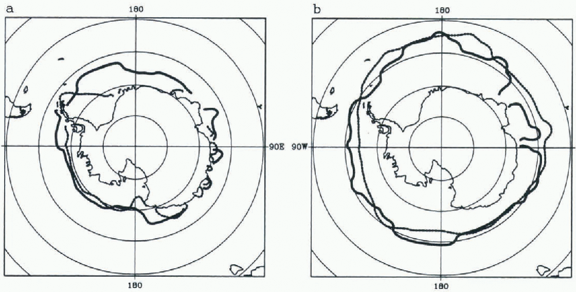
As a first step, the model is integrated in robust diagnostic mode (i.e. with volume restoring for temperature and salinity) until equilibrium is reached. After this initial stage, The relaxation is removed except in surface for salinity (see section 2) and the model is integrated for 750 years. The results presented here are averaged over the last 10 years of the experiment. Compared to the estimates of Reference Gloersen, Campbell, Cavalieri, Comiso, Parkinson and ZwallyGloersen and others (1992), the modelled Antarctic ice extent is overestimated by about 1 × 10⁶km² at the winter maximum and by about 3 × 10⁶km² at the summer minimum, which is quite reasonable (Fig. 1). During summer, the major discrepancies between model and data occur in the eastern Weddell Sea (Fig. 1a). In winter, the ice is present northwards of The observed limit in the Pacific sector of the Southern Ocean. On the other hand, the ice extent is underestimated off East Antarctica (between 45°E and 100°E) (Fig. 1b). This is due to unrealistically intense convection there, which brings heat to the surface and prevents ice formation.

Fig. 1.

The simulated (solid line) and observed (dashed line) (Reference Gloersen, Campbell, Cavalieri, Comiso, Parkinson and ZwallyGloersen and others, 1992 position of the ice edge (defined as the 15% ice concentration) in (a) March and (b) September.

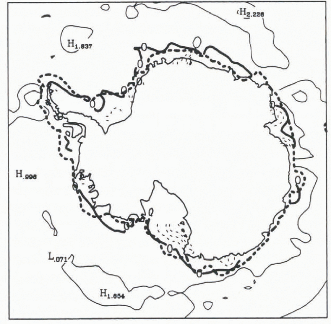
In the high latitudes of the Southern Hemisphere, the simulated annual mean fresh-water flux is generally positive (which means that the ocean gains fresh water). However, on the Antarctic continental shelf, intense ice production leads to strong negative fluxes (Fig. 2). This ice production is mainly a consequence of the winds that transport ice seawards in the vicinity of Antarctica, leaving the ocean directly exposed to the cold Antarctic air and leading to intense ice formation. Another consequence of the offshoreice transport is the existence of a quasi-circumpolar maximum in the fresh-water flux at about 60°S.

Fig. 2.

Geographical distribution of the simulated freshwater flux towards the ocean (in m a⁻¹). This flux includes precipitation, evaporation, afresh-water flux equivalent to the mass flux associated with ice melting or freezing, river run-off iceberg melting and the flux deduced from the restoring. Contour interval is 1.0 m a⁻¹; negative values are dashed and the curve corresponding to 0 is in bold. The thick dotted line represents the limit of the continental shelves (1000 m isobath) in the model.

Off the shelf, ice production is less intense. Ice divergence is generally weaker than close to the continent. Furthermore, the negative-feedback mechanism proposed by Reference MartinsonMartinson (1990) is particularly active in this zone. This process works as follows: when ice is created, salt is rejected, tending to de-stabilise the water column; this brings warm water from the deep ocean to the surface, which limits the ice growth. Note that the simulated oceanic heat flux at the ice base is generally larger in deep ocean regions than in the shelf area.

The Antarctic continental shelf is thus unique in the Southern Ocean, in the sense that it is the only region where a strong increase in salinity can occur as a consequence of negative fresh-water fluxes. The area-averaged, annual mean fresh-water budget of this zone has been estimated from model outputs. The components of this budget art-shown in Figure 3.

Fig. 3.

Simulated mean fresh-water balance of the Antarctic continental shelf (in m a⁻¹). P-E means precipitation minus evaporation. The net surface flux over the shelf (−1.03 m a⁻¹) is compensated by the net advection, the water exported being 0.19 psu saltier than the water imported.

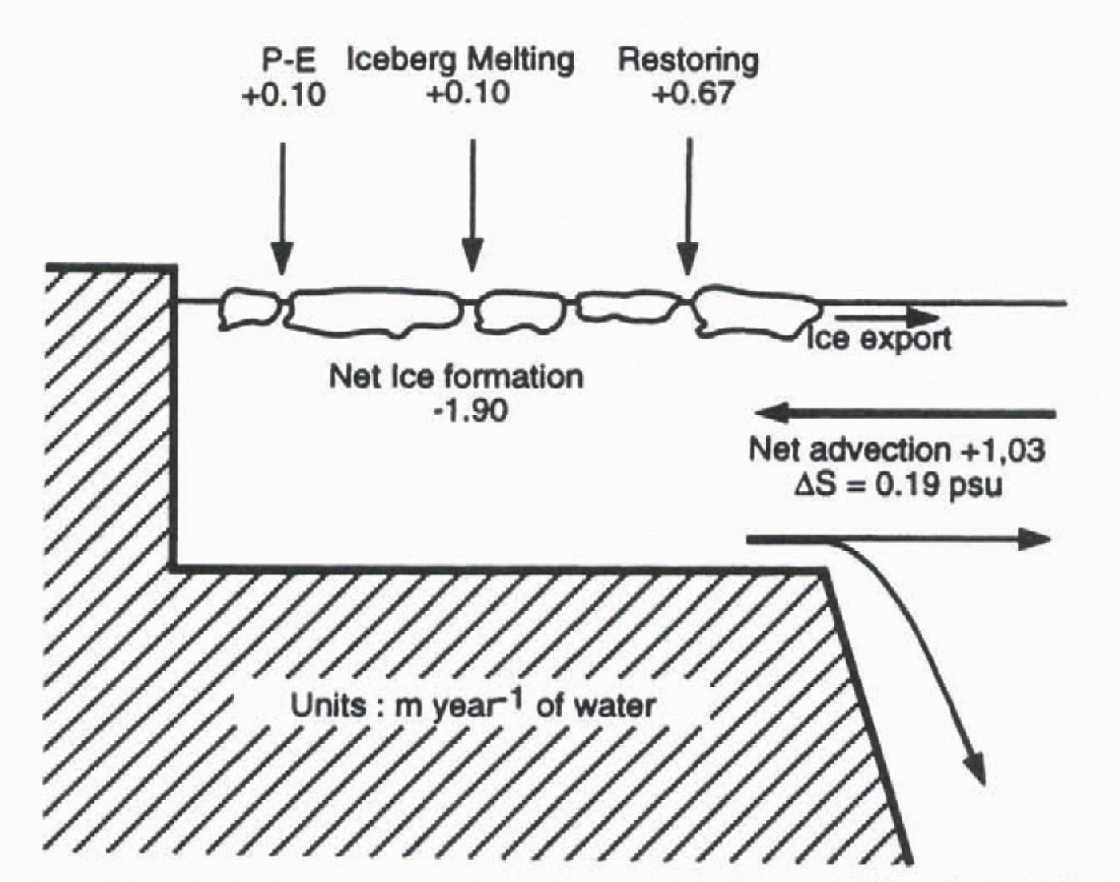
In the major part of the Southern Ocean, precipitation exceeds evaporation, as is also the case on the continental shelf (precipitation-evaporation = 0.10 m a⁻¹). In the model, we prescribe a fresh-water flux from iceberg melting of 0.10 m a⁻¹. This value has been obtained by uniformly distributing the amount of precipitation received by the Antarctic continent over the oceanic area south of 55°S (Reference Baumgartner and ReichelBaumgartner and Reichel, 1975). Anothersource of glacier fresh water comes from the melting of ice shelves. Reference Jacobs, Fairbanks, Horibe and JacobsJacobs and others (1985) deduced from various sources the total melting rate of ice shelves around Antarctica, which, distributed over the entire continental shelf, would lead to a fresh-water flux of 0.28 m a⁻¹. This flux has not been explicitly taken into account in our simulation, but will be included in the next version of the model.

The simulated net-ice production on the shelf amounts to 2.38 m a⁻¹ (corresponding to the ice exported). This induces a fresh-water flux of −1.90m a⁻¹, assuming an oceanic salinity of 34.7 psu, a sea-ice density of 900 kg m⁻³ and a sea-ice salinity of 4 psu. (For simplicity, we ignore the evolution of sea-ice salinity with time, assuming that sea-ice salinity reaches immediately 4 psu and then remains constant.) Direct measurements of ice production are not available. Reference Limbert, Morrison, Sear, Wadhams and RoweLimbert and others (1989) estimated from buoy drifts that 90% of the ice in the Weddell Sea is discharged each year in the Southern Ocean. Unfortunately, the influx from the eastern part of the Weddell Sea is not known. Furthermore, even if the sea-ice budget of the whole Weddell Sea were precisely determined, it would not be straightforward to transform it into useful information for the shelf. From a simple ice model and oceanic data, Reference GillGill (1973) proposed a net ice-formation rate greater than 1 m a⁻¹ in the Weddell Sea. Using a fresh-water budget of the Ross Sea continental shelf, Reference Jacobs, Fairbanks, Horibe and JacobsJacobs and others (1985) deduced an ice production rale of 0.95 m a⁻¹. In other model studies (e.g. Reference Stössel, Lemke and OwensStössel and others, 1990), the average net-freezing rate over the shelf is not given, rendering it difficult to carry out a comparison. A visual estimate of their results gives a value of 1–2 m a⁻¹, a little less than in our model.

The flux induced by the restoring on the continental shelf corresponds to 0.67 m a⁻¹. The restoring is stronger than in other regions, since the simulated surface salinity on the shelf is much higher than that of Levitus. The salinity exceeds 35 psu on an annual average in the southwestern Weddell and Ross Seas, values reasonable for winter but may be too high in an annual mean basis. These high salinities show that the restoring does not pose problems in our experiment on the Antarctic continental shelf, even if Levitus’ data are known to be too low there. The restoring may help to simulate the effect of ice-shelf melting not taken into account, or to compensate for perhaps a too-high ice production, or for other model deficiencies (e.g. too-simple vertical mixing, coarse horizontal resolution). As it is an integral part of the model boundary conditions, it is incorporated in our budget. Nevertheless, the non-physical nature of this flux must always be kept in mind when interpreting the results.

The simulated net-surface fresh-water flux over the Antaretic continental shelf is −1.03 m a¹. For comparison, the budget of the region of deep ocean south of 66° S is +0.29 m a⁻¹ (+0.56 m a⁻¹ south of 03 S). The value proposed by Reference Jacobs, Fairbanks, Horibe and JacobsJacobs and others (1985) from oceanic data is smaller by a factor 3 (−0.33 ma⁻¹). Reference Toggweiler and SamuelsToggweiler and Samuels 1995 deduced a flux of −0.55 m a¹ in the southernmost row of their OGCM (entirely on the shelf in their most realistic simulation. However, their model had no sea-ice component, and they used a surface-restoring boundary condition to the annual mean salinity of Levitus at 500 m in the shelf areas of the Weddell and Ross Seas and in surface Levitus’ data elsewhere. They argue that the annual mean salinity at 500 m is a good estimate of winter-surface salinities on the shelf, the mixed layer being deep at this time. The new estimate of the net fresh-water flux provided by our model is higher than the two previous ones. This value seems reliable since the model has representations of the most relevant processes, and the model results close to Antaretica agree reasonably well with observations (e.g. Fig. 1). Furthermore, none of the individual fluxes presented here is out of the range of the current uncertainly. The flux induced by the restoring max be the most problematic element of the budget. Nevertheless, if it were not included in our computation, the fresh-water flux would be even larger (in magnitude).

It is important to know the impact of this negative freshwater flux on the properties of bottom water. The −1m a⁻¹ fresh-water flux, acting over the 2.8 × 10⁶km² shelf, is equivalent to a salinity flux to the ocean of 3.1× 10⁶ kg s⁻¹, considering a salinity of 34.7 psu. Reference GillGill (1973) has proposed a value of 20 Sv for the flux of bottom water out of the Southern Ocean. A similar value may be deduced from the model results, the net northward mass-flux of bottom water at 35°S being 17.4 Sv (Fig. 4). If the whole 3.1 × 10⁶kg s⁻¹ salt flux were incorporated in this 20 Sv northw ard transport, it would cause the salinity of this water mass to increase by 0.15 psu. However, a significant part of the salt is included in the horizontal circulation close to the surface. The water remains in the top 500m, mixes with fresher water in the deep-ocean regions, and, thus, almost no transfer to the bottom is possible. Furthemore, the water sinking near the shelf slope can be diverted before reaching The bottom. To have a rough idea of the amount of salt transported from the shelf to the bottom of the world ocean, F_s we have computed the northward salt-transfer associated with the deep circulation at 65°S:

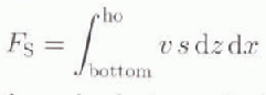
where v is the northward velocity and s is the salinity. The integration is carried out over depth (z) and longitude (x). The depth, ho, is chosen such that the mass transport between the bottom and ho is closed (no net-mass transport), i.e.:

The net salt flux is readily estimated. Furthermore, only The deep circulation is taken into account in the computatioa F_s has a value of 10⁶kg s⁻¹. If the salt flux incorporated in the northward flux of bottom water amounts to 10⁶ kg s⁻¹ rather than 3.1 × 20⁶kgs⁻¹, the effect of the surface negative fresh-water flux on bottom waters would be to the order of 0.05 psu. It shows that 0.15 psu is clearly an upper boundary. A reasonable estimate is much less than this, probably about a third of it.

Fig. 4.

Annual mean global meridional streamfunction in Sv. (a) Standard simulation. (b) Experiment WFF. Contour interval is 5 Sv. Flow is clockwise around solid contours.

4. Sensitivity Study

As described in the previous section, the impact of ice formation on the salinity of AABW is relatively weak. However, it also has an influence on deep convection, on the formation of AABW, and, more generally, on global circulation. This issue was addressed by carrying out a model experiment in which The fluxes of fresh water or salt associated with ice formation or melting are neglected hereafter called experiment WFK without fresh-water fluxes). This amounts to assuming that sea ice has the same salinity as sea water. This modification is applied only in the Southern Hemisphere to avoid perturbations coming from the north. The results of WFF are compared with those of the standard simulation after 750 years of integration starting from an equilibrium state obtained in robust-diagnostic mode (as in section 3).

In WFF, two small polynyas appear inside the pack, caused by open-water convection that generates ice melting. However, as no fresh water is associated with this melting, the convection is not reduced by a negative-feedback mechanism and can survive for a long time. The ice extent in WFF (not shown) is similar to that of the standard simulation, with only a slight increase in ice extent in winter, particularly in the region where it is underestimated in the standard experiment (i.e. off East Antaretica, Fig. 1b). When brine release during ice formation is neglected, convection strongly decreases in this area, allowing ice to form and maintain. In the standard experiment, convection in deep-ocean regions off East Antaretica is mainly generated by the advection of unrealistically high salinity water coming from the neighbouring shelves. This may suggest that ice production is too strong on the shelf. However, the too-high salinity can also be a consequence of a misrepresentation of the exchanges between the shelf area and the deep ocean (e.g. by the bottom-gravity currents). This is currently under investigation.

The annual mean net fresh-water flux at the surface of the Antaretic continental shelf amounts to 0.17 m a⁻¹ in WFF, compared to −1.03 m a⁻¹ in the standard experiment. The restoring has also changed in magnitude between the two experiments. It is very weak in WFF (0.1 m a⁻¹), the simulated salinities being close to Levitus’ data. This modification of the restoring is of a spurious nature. However, the restoring was also applied in WFF to keep The same experimental design. Using fixed fluxes diagnosed from the standard experiment in WFF, instead of restoring, was not possible since the dynamic of the system forced by fluxes or by restoring may be different. The relaxation might limit the effect of ice formation in The standard experiment (see discussion in section 3). Regardless, the difference between the two experiments is sufficiently clear to analyse the influence of the fresh-water fluxes in the model.

The shelf is much fresher in WFF (see Fig. 5 for the Atlantic) and the water is thus much less dense, the temperature being always close to freezing point on the shelf. As a consequence, the convection on the shelf and on the edge of the continental slopes ceases, except in the two polynyas, and almost no bottom-water formation takes place there. The intensity ofthe deep-overturning cell close to Antaretica decreases significantly, from 25 Sv to 15 Sv (Fig. 4). However, deep-water formation is still present in the Southern Hemisphere, as well as in open-ocean convection. Intense convection appears outside the ice pack, between 55° and 65° S. This feature is also present in the standard run. It seems to be a common problem of OGCMs using classical horizontal diffusion (Reference EnglandEngland, 1995).

Fig. 5.

Annual mean, zonally averaged salinity in the Atlantic in psu. (a) Standard simulation. (b) Experiment WFF. Contour interval is 0.2psu. Curves below 35 psu are dashed.

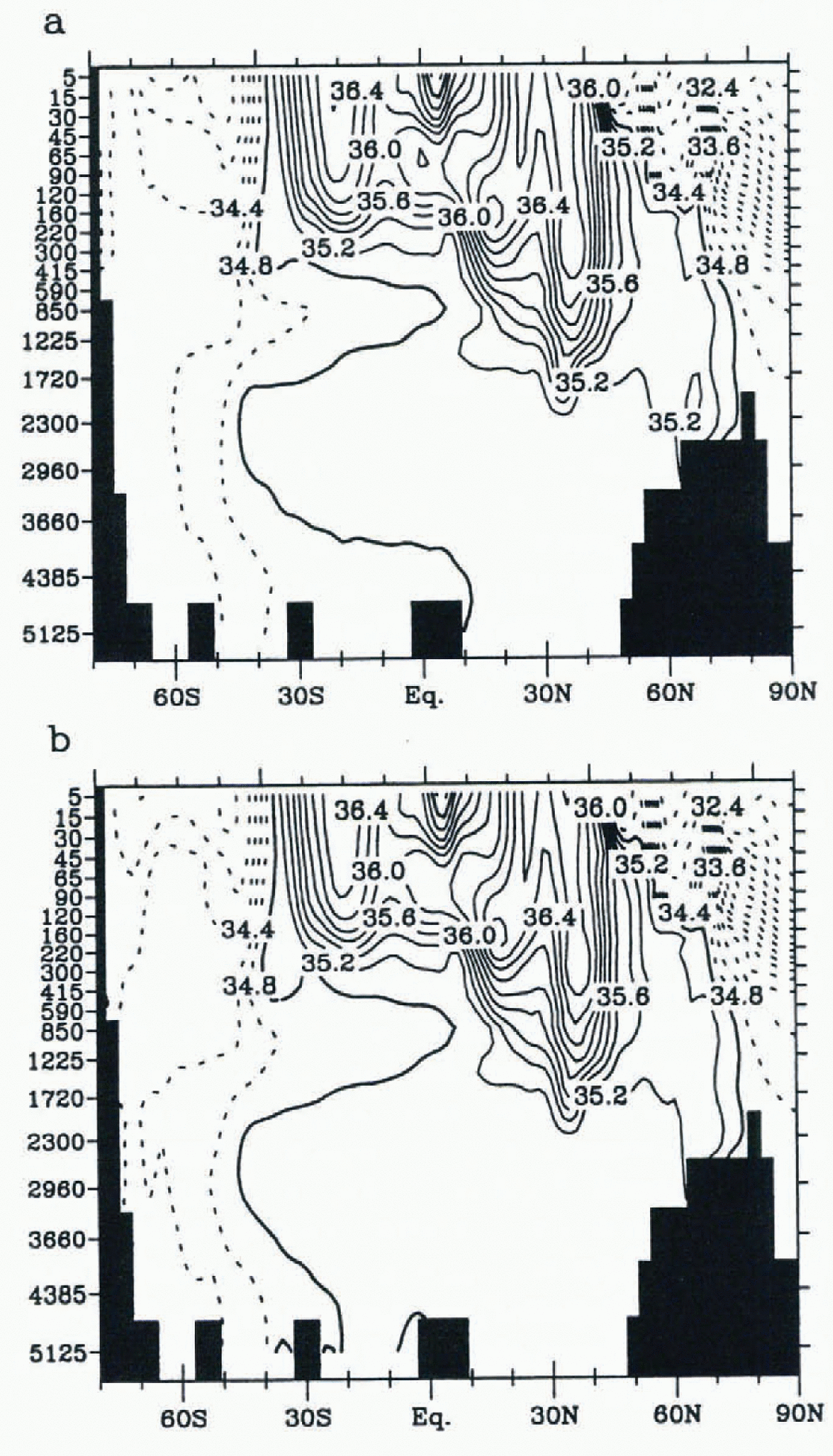
As a consequence ofthe reduction in the rale of AABW formation, the zonally averaged meridional inflow of AABW in the Atlantic at 35°S decreases from 4.3 Sv in the standard run to a little more than 2 Sv in WFF. Furthermore, AABW no longer crosses the Equator in the Atlantic, NADW reaching the bottom in the major part of the North Atlantic. The zonal average inflow below 3000 m in the Indian and Pacific oceans also decreases, from 13.1 Sv to 7.0 Sv. On the other hand, the maximum overturning in the North Atlantic increases by more than 3 Sv. The zonally averaged meridional outflow of NADW at 35°S (a measure of NADW exported to the other oceans) increases from 17.4 Sv to 20.4 Sv. There is thus a reorganisation of the thermohaline circulation, in which the decrease of AABW formation is partially compensated by an increase in the NADW overturning, the global circulation being sensitive to the density contrast between the Southern Ocean and the North Atlantic.

This modification of the circulation has consequences on the properties of water masses. On a global average, the temperature of the bottom gridcell of the model (depth 5125 m) increases from 0.79° to 1.63°C, reflecting the stronger penetration of NADW at great depths. As a consequence, the bottom waters are lighter. The decreased transport of AABW is clearly visible in Atlantic salinity distribution (Fig. 5). In the standard simulation, a fresh (and cold) tongue of AABW is propagating northwards close to the bottom beneath the salty (and warmer) NADW. In WFF, this feature is almost absent. the globally averaged bottom salinity increases in WFF from 34.70 psu to 34.76 psu. This is an unexpected result since brine release induces salt transport to the bottom in the standard experiment. It means that, considering the bottom-water salinity, the direct impact ofthe reduction of salt transfer from the shelf in WFF has a smaller influence that an indirect one, which is the supply of salty NADW.

Numerous studies have stressed the importance of the salinity near Antaretica for AABW formation and export (e.g. Reference Stocker, Wright and BroeckerStocker and others, 1992; Reference EnglandEngland, 1993; Reference Fichefet, Hovine and DuplessyFichefet and others, 1994), and for NADW formation. When the salinity near Antaretica was decreased, an increase in NADW overturning and a reduction of AABW formation were noticed. However, this modification was not associated with an increase in bottom salinity as in our experiments (Reference Stocker, Wright and BroeckerStocker and others, 1992; Reference EnglandEngland, 1993; Reference Toggweiler and SamuelsToggweiler and Samuels, 1995). This may be due to the representation of surface processes. The models did not include an explicit sea-ice model, and only part of them included a seasonal cycle. Furthermore, in our standard run, the salinity of NADW is relatively high, whereas it is underestimated in some of the other studies. This may lead to different results when the conditions around Antaretica are modified.

5. Conclusion

A study of the large-scale impact of the mass exchanges occuring during ice formation and melting has been performed with a global ice ocean model. The simulated annual mean fresh-water flux in the Southern Ocean exhibits a strong contrast between the open ocean, where a positive fresh-water flux towards the ocean is observed, and the Antaretic continental shelf, where the flux is strongly negative. This strong negative flux over the shelf is caused by net ice production. The shelf waters are thus quite Salty, with salinities much higher than the too fresh Levitus’ data, the differ ence being significant only over the shell and not over the deep ocean. As a consequence, ocean modellers, who use a restoring-boundary condition on salinity and enhance the Levilus’ data to take into account a sea-ice effect, should probably apply this correction only on the shelf (e.g. Toggweiller and Samuels, 1995).

The simulated averaged fresh-water flux over the shelf is −1.0 m a⁻¹ . This is significantly larger (in absolute value) than some previous estimates, mainly because ofthe intense ice production generated by the model in this zone. This value is within the range of cut tent uncertainty, even if inaccuracies may arise from deficiences in the model and/or in the forcing. The impact of this flux on deep water is difficult to assess. A simple argument leads to an upper boundary of 0.15 psu for the increase of the salinity of bottom water clue to the negative fresh-water flux operating over the shelf, the actual value being probably around 0.05 psu.

A numerical experiment has been conducted in which the salt- and fresh-water fluxes associated with ice formation and melting are ignored. The convection near Antarelica decreases strongly, as do the formation and export of AABW. In response to The decreased influence of AABW. there is an intensification of NADW production, which is warmer and saltier than AABW. This modification of the thermohaline circulation induces an increase in bottom temperature and. contrary to what could have been expected, an increase in bottom salinity. This means that the direct impact of neglecting the transfer of salt at great depth, which is a consequence of the brine release, is over-compensated by the higher presence of salty NADW close to the bottom. These results show that the response of the system is clearly non-linear. As a consequence, it is nearly impossible to measure the amount of salt transfered from the shell to the deep ocean by simply suppressing (or reducing) this transport and measuring the modification of bottom salinity. In our case, this method would have led to a peculiar negative salt transport from the surface to the bottom associated with ice production.