1. Introduction

What is natural selection, how do appeals to selection explain evolutionary events, and how are descriptions of natural selection to be formulated if such descriptions are to enable reliable forecasts of evolutionary outcomes; in a word, how is natural selection to be understood? For some 70 years biologists and philosophers alike have taken population genetics to provide the core formal machinery for describing and understanding natural selection and the evolutionary events it produces. I will call this the core commitment.

Population genetics does not and is not taken to provide a complete description of any instance of selection. But nearly all of philosophy of biology concerned with the conceptual foundations of evolutionary theory, and much of evolutionary biology itself, take the descriptions offered by population genetics models to be relevantly complete. Such descriptions are held to be sufficient to generalize over and hence unify episodes of selection, to provide quantitative as well as qualitative predictions about changes in type frequencies, and to explain these outcomes.

The core commitment shows itself in various ways. The consequences of selection are typically represented within the population genetics framework rather than within, say, a population regulation framework, a prima facie more plausible alternative given that what selection does, if anything, is produce differential rates of reproductive success. For example, selection is commonly understood as one among several forces driving deviations from Hardy-Weinberg equilibria rather than as a biased distribution of values over some set of variables that cause reproductive success. Or again, such measurable features as selection has are measured using the machinery of population genetics, for example, such quantities as the strength of selection, the opportunity for selection, and the response to selection.

The core commitment shows itself as well in the way the analytic or simulation results from population genetics are understood. These results are commonly constituted by qualitative constraints on allelic or genotypic frequencies at equilibrium resulting from qualitative relations between parameters in the model, for example, fitnesses, mutation rates, and effective population size. The crucial parameter related to selection in population genetics models is fitness or its analytical relative, a selection coefficient. Accordingly, to understand selection's influence on frequency change is, at least implicitly, to understand the way in which differential fitnesses lead to changes in type frequencies in contexts specified by the values of the other parameters in population genetics models.

Philosophers have by and large agreed, more or less uniformly adopting the core commitment and in practice endorsing its consequences. For those concerned with the conceptual foundations of evolutionary theory, the core commitment implicitly delimits the range of philosophical problems demanding investigation and the range of potential solutions to those problems. For philosophers, the most central of these problems is to give an adequate interpretation of the fitness parameter in population genetics models and, secondarily, to use that interpretation to formulate acceptable versions of the principle of natural selection and adequate accounts of evolutionary explanation. The influence of the core commitment is illustrated by a passage from the philosopher of biology who in distinguishing between ‘source’ and ‘consequence’ laws has come closest to relinquishing it, namely, Elliott Sober. Sober writes,

Consider the implications. The consequences of selection do not depend on the causal details by which fitness differences arise, but only the single facet of selection characterized by those differences. Predictively useful characterizations of selection must be formulated in terms of fitness differences, for it is these coefficients which are used in the consequence laws, that is, population genetics. In fact, the source laws themselves may be bits of population genetics; for example, the most frequently cited example derives from Fisher's account of sex ratios. That is no accident: source laws such as those emerging from optimal foraging theory, Fisherian or Zahavian theories of sexual selection, and other pieces of evolutionary ecology nearly always measure success with respect to some component of fitness. But there are trade-offs between components of fitness, and it is population genetics that provides the machinery for finding the optimal balance. The understanding of selection that results embodies the core commitment.

Whether an attempt to understand selection is itself regarded as a bit of biology or a bit of philosophy, most such efforts have been implicitly or explicitly framed by the core commitment. It has been a presupposition of such endeavors that to understand selection-driven evolution in a population is to have an appropriately detailed population genetics model of the population, and that abstracting from such descriptions is adequate to formulate the important generalizations about selection. I think the presupposition is in error. The task of interpreting fitness, philosophers of biology will note, has proved so enormously difficult that despite 30 years of work by some terrifically able people, we are nowhere near a plausible, much less demonstrably correct, solution. The limitations of population genetics in modeling evolutionary phenomenon are also not far to seek: for a large range of cases population genetics is both explanatorily and predictively incompetent. More, the descriptive apparatus of population genetics forces us to address a host of seriously intractable conceptual problems that otherwise do not arise at all. I think the reasons for these limitations are simple: population genetics models evolving populations with the wrong variables related by the wrong equations employing the wrong kinds of parameters.

Let me be clear about the charge. I do not mean to impugn population genetics as false, or even irrelevant. Models in population genetics serve, and serve well, for a surprising number of purposes. But I do claim that population genetics models are, on their own, inadequate to convey an understanding of selection, either in general or in particular cases, and hence are the wrong models to employ when offering an analysis of selection, abstracting from particular instances of selection to generalizations unifying disparate episodes of selection, or characterizing the nature of explanatory appeals to natural selection.

2. Predictive Incompetence

I claim that population genetics models are the wrong models in terms of which to frame an understanding of natural selection because such models are predictively and explanatorily incompetent in important respects, and their use in developing a general theory of natural selection generates avoidable conceptual confusions. In this section and the next I defend the first of these charges. Models in population genetics are predictively incompetent in two respects. They do not, in general, reliably predict the trajectory of particular populations through state-spaces defined by the frequencies of types in the population, and they do not, in general, reliably predict changes in state variables consequent to interventions on other state variables (I shall call models that succeed in this second respect causal models). Population genetics models do neither, and except in special circumstances can do neither, because they do not correctly identify or represent the dependencies between genic types, phenotypes, environmental, and demographic characteristics that generate differences in reproductive success. I begin the case with some assumptions.

First, population genetics models yield reliable predictions only if some function of absolute fitnesses of types, $\boldsymbol{f}(W_{i}) $ , reliably tracks that function of actual rates of reproductive success for the types, $\boldsymbol{f}(R_{i}) $ , where the types, indexed by i, are just those identified by the population genetics models.Footnote ¹ Just which function f is at issue depends of course on the model at hand; sometimes we are interested in absolute fitnesses, sometimes in relative fitnesses, and sometimes in more complicated functions of expectation and variance, but for every such model there is some such function. Further, what counts as ‘tracking’ depends on the context. In some contexts the demands are quite stringent: for every time t and every type i, successful prediction requires that $\boldsymbol{f}^{t}(W_{i}) \cong \boldsymbol{f}^{t}(R_{i}) $ . In other contexts, the demands are somewhat less stringent. For each time, there is for each type i some probability distribution over the values of $\boldsymbol{f}(W_{i}) $ and another over the values of $\boldsymbol{f}(R_{i}) $ at that time. On occasion it is required that at each time these distributions share a mean and a variance, and perhaps other parameters.Footnote ² In other contexts, it suffices that the distributions share a mean. But again, for every model of real populations, there is a substantive notion of tracking that must be satisfied if predictions from the model are to be reliable. Finally, I assume that, outside laboratory contexts, distributions and moments of distributions over $W_{i}$ or $\boldsymbol{f}(W_{i}) $ are estimated from small samples. Though samples may involve many, many individuals (though commonly they don't), they rarely involve many generations, typically something fewer than 100 generations, and commonly two orders of magnitude fewer.

Given these assumptions, let us note a peculiarity, and a pair of consequences. In population genetics models, fitnesses (or functions of them) are either fixed parameters or random variables drawn from some constant distribution. It follows that fitnesses and functions of them are not endogenous variables in population genetics models. That is the peculiarity: reproductive success is caused by a host of variables, but fitnesses, which must track reproductive success, are not endogenous in our models. From this peculiarity, two important consequences arise. First, when one models populations in the wild, estimates of the values of or distribution over $W_{i}$ or $\boldsymbol{f}(W_{i}) $ must be more or less direct inferences from the data; that is, one estimates the true value of or the true distribution over $W_{i}$ or $\boldsymbol{f}(W_{i}) $ directly from the sample distribution over $R_{i}$ or $\boldsymbol{f}(R_{i}) $ .Footnote ³ Second, nongenetic causes of reproductive success are not represented.Footnote ⁴ I claim it follows from either of these consequences that estimates of $W_{i}$ or $\boldsymbol{f}(W_{i}) $ are seriously unreliable: estimated values of $W_{i}$ or $\boldsymbol{f}(W_{i}) $ will in general not track true values of $R_{i}$ or $\boldsymbol{f}(R_{i}) $ . It follows that population genetics models are in general predictively unreliable. The arguments from each consequence are related but take distinct forms, so I'll give each in turn.

2.2. The Argument from Noncausal Models

The argument which follows is made more accessible by representing the causal relations governing reproductive success using the graphical causal modeling framework (Spirtes, Glymour, and Scheines Reference Spirtes, Glymour and Schienes2000). Here I give a very brief, rough, outline of the central ideas. Causal relations are taken to be asymmetric relations of dependence between variables characterizing units in a population of units. X is a direct cause of Y relative to a set S of variables and a background iff there is some pair of interventions setting the value of every variable in $\mathbf{S}\backslash \{ Y\} $ and differing only in the value of X, between which the probability distribution over Y differs. The causal structure over S is represented by a directed graph, in which there is an edge from X into Y iff X is a direct cause of Y. The full causal system includes not only the graphical representation of the causal structure but also the joint probability distribution over S, which distribution is assumed to factor according to the Causal Markov and Faithfulness conditions.

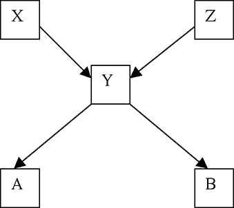
The distribution is often partly represented by a set of equations relating endogenous variables to their direct causes. In the linear case, the result is a structural equation model (SEM). For example, in Figure 1, we would write

Figure 1.

Causal structure over S.

One advantage of the graphical representation of causal structure is that it enables one to easily determine which variables will be statistically dependent, that is, associated, conditional on any other set of variables in the model. The rules for determining these dependencies are simple, deriving from Pearl's d-separation theorem (Pearl Reference Pearl2000). To use them, three definitions are useful. A variable is a mediator on a path if, in that path, there is one edge into it and one edge out (→X→ or ←X←). A variable is a common cause on a path if, in that path, there are two edges out of it (←X→). A variable is a collider on a path if, in that path, there are two edges into it (→X←). So, for example, in Figure 1 Y is a mediator on the path X→Y→A, a common cause on the path A←Y→B, and a collider on the path X→Y←Z. Here then are the rules: any two variables X and Y are associated conditional on a set V of variables iff there is some path between X and Y such that no mediator or common cause in the path is in V, and every collider on the path either is in V or has some effect which is in V. In Figure 1, the variables X and Z are unassociated if we condition on no other variables, but associated if we condition on Y, or A or B. The variables X and B are associated unconditionally, not associated if we condition on Y, but remain associated if we condition on A. A and B are associated unconditionally but unassociated conditional on Y.Footnote ⁵

Turning to the argument itself, recall that in population genetics models, fitness or functions of them are commonly introduced as fixed parameters. When this is not so, they are treated as random variables drawn from some fixed distribution. Environmental and phenotypic variables, when introduced at all, are used to constrain this fixed distribution. This implicitly assumes that the dependence relations between reproductive success and environmental or phenotypic variables are constant in form, and further that the distribution over the environmental or phenotypic variables is itself constant. Those assumptions are in general unwarranted, and in making them models in classical population genetics invite predictive incompetencies.

A population genetics model writes the collection of type frequencies at generation $g+1$ as a function m of those frequencies and fitnesses at generation g: $\mathbf{G}^{g+1}=\boldsymbol{m}(\mathbf{G}^{g},\,\mathbf{W}^{g}) +\varepsilon $ . The error term, made explicit here, arises from drift of all sorts; if it becomes too large, fitness will not track reproductive success, and in consequence the model will not be predictively useful. The size of the error depends on the extent to which G^g and $\mathbf{G}^{g+1}$ are associated, with stronger associations leading to smaller errors, and on the extent to which fitnesses correctly quantify that association (as, e.g., with the coefficients in SEMs). Error can be made unbounded in two specific ways that will concern us.

First, as in structural equation models, common causes of the exogenous variables and the endogenous variables must not be omitted. If such common causes exist and change in value, then so too will the expectations for endogenous variables. Clearly, any environmental cause of reproductive success whose value at a given generation influences its own value at later generations will constitute such a common cause, and equally clearly, variables representing these causes do not appear in the dynamical equations of population genetics models. If such common causes vary between the estimation period and the projection period, error will occur.

Second, interactive causes of the dependent variable must not be omitted. X and Y are interactive causes of Z if the effect of X on Z depends on the value of Y. Unless such interactive causes are constant in value over the projection period, changes in them may also change the joint distribution over the endogenous variable and other interactive causes (e.g., a change in Y will change the joint distribution over X and Z). To see how interactive causes matter, consider time-lagged models of population size. In populations in which population size varies cyclically, the rate of change in population size depends not simply on current population size, but also on whether the population is increasing or decreasing. This difference between years of increase and years of decrease induces a change in the form of the functional dependence between current and future population size, since there is a change in sign and also a difference between the shape of the curve on the up and down slopes of the cycle. This implies that the effect of population size now on population size in the future depends on the value of one or more other variables not included in the model itself. No single functional relation between present and future population size can reliably predict population size unless those interacting variables are included in the model. Time-lagged models of cyclical population growth typically involve two functional relations, one characterizing growth during years of increase and a second during years of decrease, and use the lags to induce switching between the regimes.

If fitnesses are to reliably track rates of reproductive success, values for the latter must be drawn from a constant distribution, with roughly the same form and with roughly the same statistical parameters as that from which the corresponding fitnesses are drawn. But this cannot be so if rates of reproductive success have interactive causes whose values vary over the projection period, since such variation will ‘switch regimes’, that is, change the distribution over particular rates of reproductive success $R_{i}$ .

Aside from the evidence from population regulation, there are good reasons to think there are interactive causes of rates of reproductive success. I'll make the case here with respect to a particular behavioral variable, but the idea is perfectly general. Behaviors are environmentally sensitive in two ways. First, there are sensitivities described by ‘choice rules’: when in environment E do b, when in $\boldsymbol{E}^{\prime }$ do $b^{\prime }$ . The pattern of behaviors an individual exhibits, say in prey selection, can be described by such choice rules. But sometimes it is advantageous to be able to switch back and forth between choice rules over time. Call a rule for switching between choice rules a meta-rule. Take meta-rules to be, by definition, fixed for an individual over its life span, while choice rules need not be. Foraging theory provides a nice example of an advantageous meta-rule.

Let $K_{1}$ – $K_{n}$ be a list of potential prey items, ordered in decreasing profitability. According to optimal foraging theory, potential prey items ought elicit attack from a predator either always or never (the so-called zero-one rule). Whether or not items of kind $K_{k}$ ought to elicit attack depends on the energetic demands of the predator, the profitability of $K_{k}$ , and the profitability and frequencies of prey items of kinds $K_{1}$ – $K_{k-1}$ . The kinds upon which a predator in fact preys identify a choice rule under which it is operating: ‘Prey on items of type $K_{1}$ – $K_{k-1}$ if opportunity arises, but never on items of kinds $K_{k}$ – $K_{n}$ '. If the frequencies of items of kind $K_{1}$ – $K_{k-1}$ decrease, then the choice rule ought to change—items of lower profitability ought to be added to the diet. The rule for adding or removing items from the list of those preyed upon is, in our terms, a meta-choice rule; when the choice rules adopted by individual predators over the course of their lives change with time according to a meta-choice rule, there will be interactive causes of reproductive success. The frequency of $K_{2}$ in the current generation is an interactive cause of reproductive success in that generation for any type that employs the meta-rule: the frequency of $K_{2}$ has an effect on reproductive success if, but only if, the frequency of $K_{1}$ is sufficiently low; hence the frequency of $K_{1}$ in the current generation is also an interactive cause of reproductive success in the current generation.

Prey selection is a particular case, but there is nothing very special about it. Choice rules imply dependencies between environmental variables $\mathbf{E}_{c}$ and behavior b. Meta-choice rules, when they exist, imply that these dependencies are interactive: the dependency between $\mathbf{E}_{c}$ and b changes form as a further set of environmental variables $\mathbf{E}_{m}$ change in value. If b is a cause of reproductive success, then $\mathbf{E}_{m}$ and $\mathbf{E}_{c}$ will be interactive causes of reproductive success. Indeed, there is nothing very special about behaviors; these kinds of causal dependencies can equally well hold with respect to polyphenisms and phenotypic plasticities. Meta-choice rules should evolve whenever the optimal behavioral or phenotypic response to an environmental signal varies with environments and the cost of learning is small. Those conditions will not always be met, but they are not particularly restrictive, so it is likely they will commonly be met. When they are, classical population genetics models will fail predictively.

3. Objections: Markov Models and the Exception That Proves the Rule

Both the argument from direct estimation and the argument from noncausal models exploit a pair of facts: the causes of reproductive success vary over generational time, and the dependence relations between these causes and reproductive success are not represented in population genetics models. More predictive models, it would seem, will therefore require explicitly causal models of selection. Two objections arise immediately. The first of these takes the following form. It might be true that population genetics ignores much causal detail at the individual level, but it does so legitimately. Such causal detail is so much micro-causal noise. In real populations most of this noise cancels out, so that the behavior of particular populations is closely approximated by a diffusion or branching process whose macro-level statistical behavior can be captured without any causal representation. This objection is mistaken.

It may be true that in reasonably large populations the behavior of the population is approximated by, say, a mathematical description in terms of some diffusion process. But there are two things to note. First, the predictions generated from such models typically depend on the assumption that the population is Markov in the state variables for the model; that is, the future state of the population is statistically independent of its past state, conditional on its current state. The state variables are in G, and populations are almost never Markov in G. The Markov condition will be violated whenever there is an environmental variable, say the frequency of some predator, whose value at $t_{1}$ is an effect of variables in G at $t_{0}$ and a cause of variables in G at $t_{2}$ : we then have a path $\mathbf{G}^{0}$ →V→ $\mathbf{G}^{2}$ which induces an association between $\mathbf{G}^{0}$ and $\mathbf{G}^{2}$ even when conditioning on $\mathbf{G}^{1}$ , since V is not in $\mathbf{G}^{1}$ . There are nearly always such variables, as indicated by the common necessity of introducing lagged models of population growth. Second, given that a population is not Markov in the state variables, then even to the extent that the models do predict the behavior, they will misrepresent why this behavior occurs.

But there are exceptions. A second objection appeals to an undoubted predictive success of population genetics models, the prediction of sex ratios in diploid species. Sex ratios are a special kind of equilibrium, one that results from stable frequency or density-dependent selection. Suppose, as with sex ratios, selection works against the more frequent type, so that $W_{C1}> W_{C2}$ iff $\mathrm{Fr}\,(C1) < \mathrm{Fr}\,(C2) $ . Then the qualitative relations between fitnesses depend on selection pressures which themselves depend on class frequencies; that is, class frequencies are the dominant variables causally influencing reproductive success. Since these class frequencies are represented in the population genetics model, the model is able to predict the consequences for fitness of changes in values among causes of reproductive success. Hence the model is able to reliably predict the existence of an equilibrium in the population over long temporal spans and over wide ranges in values for other relevant variables. Moreover, in the case of sex ratios, while changes in other relevant background variables may shift the equilibrium value, they commonly do so without changing the fact that there is always some equilibrium. That is, the dependencies between reproductive success and class frequencies represented by the model are relatively stable. Consequently the models provide useful law-like regularities covering those shifts in equilibrium value. In short, population genetics models enable reliable predictions of sex ratios exactly because, in such cases, they are causal models: type frequencies, represented by variables that do appear in the model, are causes of reproductive success, and those causal relations are relatively stable.

For many predictive tasks of interest, the success of population genetics models turns out to depend on whether or not those models are causal. Such models are causal only in special cases, and so in general fail to yield reliable predictions for a large range of important cases. As it turns out, much the same is true with respect to explanatory success.

4. Explanatory Incompetence

There are two current conceptions of evolutionary explanations. On one increasingly popular conception, evolutionary explanations are essentially statistical and noncausal (Walsh, Lewens, and Ariew Reference Walsh, Lewens and Ariew2002; Matthen and Ariew Reference Matthen and Ariew2002). On this statistical conception, evolutionary explanations aim to explain the ‘central tendencies’ of a population's trajectory through geno- or pheno-space by appeal to the statistics describing reproductive rates among classes and the distribution among types of the offspring produced by matings between parents with specific genotypes. These explanations are not causal, being explicitly independent of the causal relations generating the statistical patterns to which explanantia appeal.

Differently, one can agree that evolutionary explanations take central tendencies as their explananda, but nonetheless insist that such explanations are essentially causal. This is, I suppose, the dominant tradition, and so I shall call it. On this view evolutionary explanations appeal to population-level type causes to explain the central tendencies exhibited by populations in their trajectories through geno- or pheno-space (Sterelny and Kitcher Reference Sterelny and Kitcher1988). Accordingly, deviations from expectations are regarded as a matter of drift, in one or another sense, and not otherwise explicable, but the expectations from which these deviations are deviations result from causal influences summarized by parameters whose values represent fitness, migration, mutation, and so on. Since actual frequencies are causal consequences of causes whose net expected effect is represented by the parameters in the model, population genetics models provide causal explanations of frequencies, at least when those frequencies reasonably approximate expectations. Or so the story goes.

The statistical conception of evolutionary explanation has been defended largely by criticizing the dominant tradition on two grounds. Both lines of criticism challenge the idea that fitness, understood as a propensity, can underwrite causal explanations. On the first line of critique, fitnesses are noncausal (Walsh et al. Reference Walsh, Lewens and Ariew2002; Matten and Ariew Reference Matthen and Ariew2002). On the second, fitnesses are nonexistent; there is no underlying fitness property to be measured by any fitness parameter (Ariew and Lewontin Reference Ariew and Lewontin2004). In the context of the core commitment, either charge underwrites the further claim that evolutionary explanations are noncausal.

I do not think either line of objection is quite right, and in any case both overlook the really important difficulties facing the dominant perspective. But even were these objections right, the statistical conception of evolutionary explanation offers little improvement, unless much, even most, of what population biologists do in their explanatory practices is simply otiose. Field biologists care about vera causa principles when generating selection explanations. Consider a pair of particularly well-known cases. Grant (Reference Grant1986) and colleagues are at pains to show that beak morphology in fact causes mortality—how else to understand the importance in their work of Price's modeling, of measures of seed hardness and availability, and so on? Endler (Reference Endler1980) is at pains to show that coloration has effects on mate choice and predation frequency in the lab and in the wild. Why should he care, unless he cares what the facts about causation are? It is hard to make sense of the effort, time, and money spent to show that morphological traits thought to be under selection actually do causally influence components of fitness, and hence reproductive success, except under the assumption that biologists think causation matters to their explanatory endeavors. But if this is so, the statistical conception of evolutionary explanations is at best only part of the story and is simply wrong in claiming that the causal details are irrelevant, only central tendencies matter.

Herein lies one of the several serious difficulties with the dominant view, and the propensity interpretations of fitness used to buttress it. The causal explanations of interest in evolutionary biology are not exhausted by those which appeal to type-level population causes. That, for example, beak morphology is a type-cause of reproductive success in the Galapagos environment is relevant, but incomplete, with respect to some of the questions Grant and Price are trying to answer, namely, did beak morphology actually cause reproductive success for individual birds during the study period, and did such actual causal relations occur with sufficient frequency to account for changes in population frequencies in the study populations? Those questions, and the explanatory use of their answers, are sensible only on a conception of evolutionary biology according to which part of the job is to answer questions about patterns of actual causation between individuals and aspects of their environment. Relations of actual causation cannot be identified without prior identification of causal relations between variables, even though the latter does not suffice for the former. Hence, even the dominant tradition does not go far enough in its commitment to causal representations of selection.

The failures of the dominant and statistical conceptions of selection explanations are consequent to two facts. The first is that population genetics models are, in general, noncausal models. A model is causal to the extent that it generates reliable predictions about the values variables in the model take consequent to ideal interventions on other variables in the model. Population genetics models generally do not do this: interventions that set class frequencies to something other than zero or one will in general modify fitnesses, and those modifications are not predictable from the model itself, since the fitnesses are not endogenous variables in the model. For example, interventions on the frequencies of genetic classes will induce changes in class fitnesses whenever demographic variables causally influence survival and reproductive success. In such cases, interventions on the frequencies of genetic classes produce changes in fitnesses because the distribution of demographic variable values over the genetic classes after intervention need not, and typically will not, mirror the distribution prior to intervention. The new sample distribution of the demographic variable values will influence indirectly the probability distribution over rates of reproductive success for each class, but will not be reflected by fitnesses when those are treated as fixed parameters or exogenous variables.

The second fact is that the dominant and statistical conceptions are both driven by the core commitment, by the idea that the formal machinery of population genetics provides relevantly complete descriptions of selection processes. The two conceptions of explanation differ only over the appropriateness of causal interpretations of the equations in population genetics models, and hence of the explanations they generate. On both conceptions, those equations and no others are required for explaining central tendencies. In this, both conceptions err: the statistical conception in taking causal explanation to be irrelevant, the dominant conception in taking causal interpretations of population genetics models to be cause enough.

5. Alternative Modeling Strategies

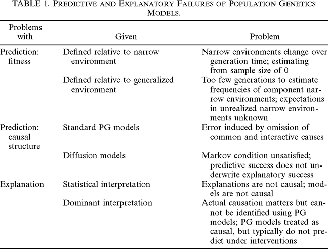
The predictive and explanatory failures of population genetics models as diagnosed so far are briefly recapitulated in Table 1. I take them to show that explicitly causal models of selection are required for a fully competent theory of evolution by natural selection. Sample distributions over rates of reproductive success do not contain enough information to reliably estimate future rates of reproductive success, but sample distributions over rates of reproductive success and variables representing their genetic, phenotypic, and environmental causes do, sometimes, contain enough information to reliably infer causal models of reproductive success. Such models enable reliable prediction and constitute the kind of causal description required for explanatory endeavors characteristic of biological practice. What will such models look like, in what sense will they represent selection, and how can unifying generalizations be abstracted from such representations?

Table 1.Predictive and Explanatory Failures of Population Genetics Models.

Problems with	Given	Problem
Prediction: fitness	Defined relative to narrow environment	Narrow environments change over generation time; estimating from sample size of 0
	Defined relative to generalized environment	Too few generations to estimate frequencies of component narrow environments; expectations in unrealized narrow environments unknown
Prediction: causal structure	Standard PG models	Error induced by omission of common and interactive causes
	Diffusion models	Markov condition unsatisfied; predictive success does not underwrite explanatory success
Explanation	Statistical interpretation	Explanations are not causal; models are not causal
	Dominant interpretation	Actual causation matters but cannot be identified using PG models; PG models treated as causal, but typically do not predict under interventions

Whatever the mathematical form of a model, algebraic or statistical or what have you, a model will be causal only if it specifies the pairwise asymmetric relations of direct causal dependence between state variables. Such relations can be represented by directed graphs over state variables, whether or not a given model employs this machinery. Definitions of relevant selection concepts can be formulated using a graphical representation, at the level of either individuals or populations. Here I develop a set of definitions assuming models of the former kind, restricting attention to the causal structure over reproductive success; below I consider in passing models of the second kind which involve no such restriction.

Say that a causal graph is correct but possibly incomplete if, where S is the set of variables in the graph and X and Y are arbitrary members of S, there is a directed edge from X to Y if and only if X is a direct cause of Y relative to S. Such graphs are correct in the sense that they include and correctly orient all edges between variables in S, but possibly incomplete in that causes of variables in S may themselves be omitted from S. Let P be a population, and let C be a causal graph that is a correct but possibly incomplete representation of the causal structure governing reproductive success, R, for individuals in the population.Footnote ⁶ Then we can say there is selection on P just in case in some C there is at least one directed path from at least one genotypic variable T to R, and T varies in value over the population; further, we can say that there is selection on a trait-variable T, just in case there is some C in which there is a directed path from T to R, and T varies in value in the population. We can then take a selection process to be a path in some C from some trait-variable T to reproductive success R, and we can take such a process to constitute selection on a particular trait-value t of T just in case an intervention changing the value of T from t to $t^{\prime }$ , but directly affecting no other cause of R, would change the distribution over R. Extensions to notions of ‘selection for’ and ‘selection against’ require contextualization by a specific contrast: there is selection for t as against $t^{\prime }$ just in case an intervention changing the value of T from t to $t^{\prime }$ , but directly affecting no other cause of R, would increase the expected value of R.

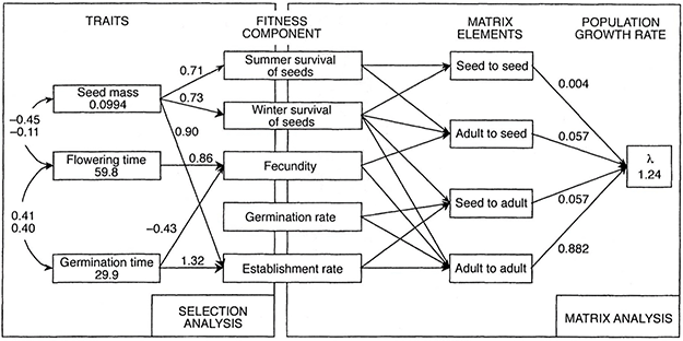
Given the prevalence of ‘population-level’ thinking in philosophy of biology, some may worry that the above definitions of selection are inappropriately reductive in that they focus on individual-level causal phenomena. I am not at all sure that such reduction as is implied by the above definitions is out of place. But in any case, it is inessential, since population-level formulations of the same basic ideas are possible. The closest things to explicitly causal, global models of selection in population biology, so-called ‘hierarchical’ models, are so formulated. The basic idea is relatively straightforward. Induce a demographic structure by dividing a population into demographic groups defined by spatial location and stage or age. Represent the structure of causal influences between demographic groups by a directed graph over variables representing the size of these groups. With each edge in the graph, associate a parameter representing transition rates between distinct demographic groups directly connected by the edge, estimated from the data. Use these parameters to build a projection matrix model of the population. Such models predict population size and demographic structure. Because the average fitness in a population is typically related in straightforward fashion to changes in population size, projection matrix models offer the opportunity to measure quantitatively the effect of particular components of fitness on group-to-group transition rates, and hence on overall reproductive rates. One can then build a causal model of the effect of phenotypic or environmental variables on components of fitness using path analysis or regression methods. Introduced by van Teinderen (see van Teinderen [Reference van Tienderen2000] for an elegant introduction and Coulson et al. [Reference Coulson, Kruuk, Tavacchia, Pemberton and Clutton-Brock2003] for an extension to environmental variables), such ‘hierarchical models’ are essentially causal models representing the ways in which phenotypic and environmental variables influence reproductive success. A graph representing such a model, taken from van Teinderen (Reference van Tienderen2000), is reproduced in Figure 2.

Figure 2.

From van Tienderen (Reference van Tienderen2000, 674).

I do not mean here to endorse the particular procedures recommended or employed by van Teinderen or Coulson et al. There are difficulties, or at least questions, about the adequacy of the methods: it is not clear how the choice of demographic variables is best constrained, whether elasticities or sensitivities or something else are the right statistics for edge loadings; and there are substantive questions about model selection for every independent piece of the model. But I do want here to recommend the general strategy. If a predictive and explanatory theory of natural selection is to be had, it will require formulation in terms of models that, like hierarchical models, explicitly represent the environmental, phenotypic, and genotypic causes of reproductive success.

Models of selection, in the sense here proposed, invite generalizations that are simply unavailable without such models. For example, it may be that particular variables—those corresponding to particular environmental, phenotypic, or genotypic features or to particular demographic features or to particular components of fitness—are commonly related to reproductive success by particular causal structures or involve dependencies of a particular form or sign. Or again, several such variables may commonly be related by a particular structure or system of dependencies. Differently, it may be that particular causal structures, when realized, reliably produce particular qualitative phenomena, for example, cycles, chaotic patterns, shifting equilibria, and so on. One cannot know beforehand whether any interesting generalizations are there to be found, of course. This depends on which variables are related by which causal structures, and the form of those relations, in biological populations. But one cannot know at all until explicitly causal models of those populations are developed. The absence of such models, and hence of generalizations over them, is relevant not just for biologists (cf. Endler and McLellan Reference Endler and McLellan1988) but for philosophers of biology as well. For example, the lacuna ought to be regarded as a serious problem by those who think there are few or no truly nomic regularities in evolutionary biology. Further, causal models of reproductive success provide a means to compute the relative superiority of alternative life-history strategies, allowing the calculation of the net effect of various trade-offs without appeal to population genetics models. They thereby provide a further source for generalizations across distinct episodes of selection.

6. Conceptual Confusions Avoided

If, in contrast to the core commitment, causal models are taken to provide the core formal machinery for describing processes of natural selection, a number of long-standing conceptual worries disappear, and others at least seem to be susceptible to solution. Most clearly, worries about finding some general interpretation of fitness disappear. Since the unified description of selection processes produced by population genetics, such as it is, is no longer also the description in terms of which we are to understand selection as an evolutionary force, there is no reason for a notion of fitness common to all such models. Adopting different definitions for different contexts is not problematic unless we equivocate by identifying the fitness parameters on each occasion of use. Such equivocation is at least suggested when the core theoretical description of selection processes is provided by population genetics. It is not even intimated if selection processes are described by causal models.

Somewhat less obviously, a host of incoherencies about the relation between selection and drift simply disappear. To pick one, the idea that there is an ‘effect’ of drift, different from and sometimes opposed to that of selection, is clarified. The idea is nonsense. Consider possible instances of drift. Is a case of sampling error an instance of drift? If so, then drift is not a cause and can have no effect; sampling error is, by definition, uncaused. Is a case of sample bias an instance of drift? If so, drift is not something other than selection; it is merely a selection process not represented by a given model, since bias is, by definition, produced by cause whose causal influence on the response variable is not represented in the model. Consider a case in which no actual cause of reproductive success in the population is an instance of any relevant causal generalization (as, e.g., when the variables whose values are actual causes of death have zero variance in the population: Igor but not his twin is killed by a lighting strike before either reproduces). Is this case also an instance of drift? If so, then drift and selection cannot be ‘opposed’ in any interesting sense: causal generalizations and claims about actual causation are different in kind, presupposing as they do a different framework for causal judgments. Or again, are rates of reproductive success which result from some especially unlikely set of initial conditions a case of drift? If so, selection and drift are not opposed, indeed not even distinct: drift is then the result predicted by our model of selection when improbable initial conditions, that is, unlikely values for exogenous variables, occur.

7. Conclusion

Population genetics gives us a set of extraordinarily useful devices for representing frequency changes in natural populations and for describing selection processes. Those uses remain important, even essential, in much of evolutionary and population biology. But, largely as an historical accident, many biologists and nearly all philosophers have overinvested in population genetics, in that, implicitly or explicitly, population genetics is taken to provide the core formal machinery for describing selection processes. This core commitment has led to a conception of evolutionary modeling on which evolutionary biology cannot predict many phenomena of interest and can predict others only under special conditions. It has led biologists and philosophers alike to misrepresent the structure and aim of evolutionary explanations, reading them as causal explanations of the wrong explananda or, worse, as noncausal explanations. And finally, it has led to avoidable conceptual confusion.

Better representations of evolutionary phenomena and their causes are, in principle, to be had by appeal to explicitly causal models and parameterizations of them. Such models ought to permit better predictions; they will make sense of explanatory demands and explanatory practices in biology; and they offer conceptual resources to resolve a number of long-standing philosophic puzzles, not least those of defining selection, interpreting ‘fitness’, and distinguishing the effects of selection from those of drift.

Replacing population genetics models with causal models as our core machinery for describing and understanding selection invites other concerns, in particular epistemological problems regarding model discovery, selection, and identification. These problems are not trivial and, if not legion, then anyway numerous. Even so, they have an advantage over those we inherit from the last three decades of work in philosophy of biology. Being epistemological rather than metaphysical or interpretative, one can at least hope for a definitive resolution of them.