


1. Introduction
This study aims to understand the mechanisms that generate various structures of secondary flows in particle-laden gas–solid flows within horizontal pipes, for which there is currently no consensus. Here, a secondary flow is defined as the mean motion in the cross-sectional plane of the pipe, perpendicular to the mean streamwise flow direction. In the literature, it is generally accepted that the generation of secondary flows of the continuous fluid phase can be classified into two different categories, depending on the driving mechanisms (Speziale Reference Speziale1982). Secondary flows of the first kind are driven by external forces, such as external pressure gradients, buoyancy forces or moving particles (Alletto & Breuer Reference Alletto and Breuer2013). For example, secondary flows can be driven by the centrifugal force in curved pipes (Noorani, El Khoury & Schlatter Reference Noorani, El Khoury and Schlatter2013; Kalpakli Vester, Örlü & Alfredsson Reference Kalpakli Vester, Örlü and Alfredsson2016; Wang et al. Reference Wang, Örlü, Schlatter and Chung2018; Chin et al. Reference Chin, Vinuesa, Örlü, Cardesa, Noorani, Chong and Schlatter2020) or the buoyancy force in heated pipes/channels (Yao Reference Yao1978a,Reference Yaob; Sekimoto et al. Reference Sekimoto, Kawahara, Sekiyama, Uhlmann and Pinelli2011; Tian et al. Reference Tian, Wei, Dai, Song and Shi2019). Secondary flows of the second kind are associated with the anisotropy of the Reynolds stress tensor in the pipe cross-section and thus by turbulence itself, such as those in non-circular pipes (Speziale Reference Speziale1982; Dykhno, Williams & Hanratty Reference Dykhno, Williams and Hanratty1994; Galletti & Bottaro Reference Galletti and Bottaro2004; Larsson et al. Reference Larsson, Lindmark, Lundström and Nathan2011), in circular pipes with a non-uniform roughness (Hinze Reference Hinze1973; Van't Westende et al. Reference Van't Westende, Belt, Portela, Mudde and Oliemans2007) and stratified flows (Flores, Crowe & Griffith Reference Flores, Crowe and Griffith1995; Vollestad, Angheluta & Jensen Reference Vollestad, Angheluta and Jensen2020). The particles transported within pipe flows can also induce a secondary flow. Specifically, secondary flows in particle-laden flows can be generated directly by the particle forces exerted on the fluid, which correspond to a secondary flow of the first kind. Alternatively, secondary flows in particle-laden flows can be induced indirectly by the inhomogeneous distribution of the particles over the pipe cross-section, as it leads to an inhomogeneous turbulence attenuation and an anisotropy of the Reynolds stress tensor. Such secondary flow corresponds to a secondary flow of the second kind. However, a lack of information is available from the literature to fully classify the potential types of secondary flows in horizontal particle-laden pipe flows, particularly those that can occur under different flow regimes (i.e. based on different flow parameters). Additionally, the information available is also insufficient to identify all of the mechanisms that may be present, because the particle forces exerted on the fluid and anisotropic Reynolds stresses do not necessarily occur in isolation. That is, a secondary flow may be of both the first and second kinds.
The necessary and sufficient conditions for the presence of secondary flows in particle-laden pipe flows within a two-dimensional cross-section have been derived from the three-dimensional Navier–Stokes (N–S) equations by Belt, Daalmans & Portela (Reference Belt, Daalmans and Portela2012), given by
 \begin{equation} \boldsymbol{\nabla} \times (\boldsymbol{\nabla} \boldsymbol{\cdot} \tilde{\boldsymbol{\tau}}_{y-z}) + \boldsymbol{\nabla} \times \boldsymbol{S}_{p,y-z,0}\neq 0, \end{equation}
where  $\tilde {\boldsymbol {\tau }}_{y-z}$ is the projection of the Reynolds stress tensor onto the cross-section (with the subscript ‘
 $y-z$’), while
 $\boldsymbol {S}_{p,y-z,{0}}$ is a component of the cross-sectional fluid–particle interaction force exerted on the fluid that is independent of the secondary flow (with the subscript ‘
 $0$’, explained in detail by Belt et al. Reference Belt, Daalmans and Portela2012). Note that here,
 $\boldsymbol {S}_{p,y-z,{0}}\equiv \boldsymbol {S}_{p,y-z}(\boldsymbol {u}^{f}_{y-z}= 0)$, where
 $\boldsymbol {u}^{f}_{y-z}$ is the cross-sectional fluid velocity. Both
 $\tilde {\boldsymbol {\tau }}_{y-z}$ and
 $\boldsymbol {S}_{p,y-z}$ are the source terms for the vorticity
 $\boldsymbol {\omega }_{x}$, which is a scalar for the two-dimensional velocity field
 $\boldsymbol {u}^{f}_{y-z}$:
 \begin{equation} \rho^f\,\frac{\mathrm{D}\omega_{x}}{\mathrm{D}t} = \mu\,\nabla^2\omega_{x} + \boldsymbol{\nabla} \times (\boldsymbol{\nabla} \boldsymbol{\cdot} \tilde{\boldsymbol{\tau}}_{y-z}) + \boldsymbol{\nabla} \times \boldsymbol{S}_{p,y-z}, \end{equation}
which is obtained by applying the curl to the two-dimensional N–S equation. Here,  $x$,
 $y$ and
 $z$ denote the streamwise, lateral and vertical directions, respectively, in the Cartesian coordinate system of the flow. Also,
 $\rho ^f$ and
 $\mu$ are the fluid density and dynamic viscosity, respectively. Therefore, in (1.1), a secondary flow driven by a non-zero
 $\boldsymbol {\nabla } \times \boldsymbol {S}_{p,y-z,{0}}$ corresponds to that of the first kind, while a secondary flow driven by a non-zero
 $\boldsymbol {\nabla } \times (\boldsymbol {\nabla } \boldsymbol {\cdot } \tilde {\boldsymbol {\tau }}_{y-z})$ corresponds to that of the second kind (Belt et al. Reference Belt, Daalmans and Portela2012). However, in this equation, it is not necessary that only one of these two terms on the left-hand side is equal to zero, which means that both can induce a secondary flow, as mentioned earlier. Additionally, the component
 $\boldsymbol {S}_{p,y-z,{0}}$ is not easy to isolate from
 $\boldsymbol {S}_{p,y-z}$, as the fluid–particle interacting forces are strongly coupled through the slip velocity. Hence the theoretical term in (1.1) is difficult to isolate. Furthermore, a Reynolds stress is, by definition, derived from the Reynolds-averaging process rather than from the instantaneous forces. To the best of the authors’ knowledge, no previous study has gone beyond the analysis of Reynolds stresses to assess the role of these instantaneous forces on secondary flows in particle-laden flow systems.
For particle-laden flows in horizontal pipes, several studies have reported various structures of the secondary fluid flow and proposed their causes. The key information of these previous studies is summarised in table 1. For instance, Sommerfeld & Lain (Reference Sommerfeld and Lain2009), Lain, Sommerfeld & Quintero (Reference Lain, Sommerfeld and Quintero2009) and Lain & Sommerfeld (Reference Lain and Sommerfeld2012) have reported a structure with two cells (anticlockwise on the left and clockwise on the right) or with four cells (with the above-mentioned two cells below and two contrary cells above) for secondary fluid flows under simulations performed with or without inter-particle collisions. The mass loading in their study was varied from  $\varPhi _m=1.0$ to
 $\varPhi _m=8.8$, which corresponds to a particle volumetric fraction within the transition between the two-way coupling (where the conveying fluid and particle motions influence each other) and four-way coupling (where inter-particle interactions are also significant) regimes. They attributed such secondary fluid motions to the momentum transfer from particles, which implies a secondary flow of the first kind, because particles collide with the circular pipe wall and therefore rebound back towards the core of the pipe (the so-called focusing effect of Sommerfeld & Lain Reference Sommerfeld and Lain2009). Moreover, the upper two of the four cells were deduced to be generated as a result of inter-particle collisions, which enhance the vertical dispersion of particles and increase the collision frequency between particles and the upper pipe wall. Nonetheless, the secondary particle motions in their study were not reported to verify this.
Previous studies on secondary flows in horizontal particle-laden pipe flows. Here, * denotes estimates by the current authors from the data reported in the original papers. Note that  $Re^f_b$ is the bulk fluid Reynolds number,
 $Sk$ is the Stokes number,
 $\varPhi _m$ is the particle mass loading,
 $\rho _r$ is the particle-to-fluid density ratio, and
 $Fr$ is the Froude number. Also,
 $e_{p-w}$ and
 $e_{p-p}$ are the coefficients of restitution of particle–wall and inter-particle collisions, respectively. The wall roughness is characterised by the standard deviation of the roughness angle distribution (depending on particle size and roughness height),
 $\varDelta \gamma$, or the wall roughness height in wall units,
 $k^+_s$. The secondary flow structures are illustrated in figure 1. The configuration of the present work in the last row is described in § 2.2.

Later studies have revealed secondary flows of the second kind for particle-laden flows in horizontal pipes. An experimental study by Belt et al. (Reference Belt, Daalmans and Portela2012) employed fixed, non-uniformly distributed particles in a fully developed horizontal pipe flow to isolate from other phenomena the fluid–particle interaction forces, which have the potential to generate secondary flows of the first kind. They observed a structure with four cells (two dominant centre-upward cells below, and two elongated cells near to the upper pipe wall). This secondary flow structure was attributed to the anisotropy of the Reynolds stresses induced by non-uniformly distributed particles. Therefore it is a secondary flow of the second kind. The large-eddy simulations (LES) study by Alletto & Breuer (Reference Alletto and Breuer2013) obtained only a two-cell (clockwise on the left and anticlockwise on the right) secondary flow structure, regardless of the mass loading  $0.3\leq \varPhi _m \leq 0.7$ (corresponding to the top of the range for the two-way coupling regime). They excluded the possibility that the continuous fluid phase is driven by the particles, based on the analysis of the particle drag forces. Instead, the inhomogeneous particle distribution was reported to result in anisotropy of the Reynolds stresses in their simulation, thus also being associated with the secondary flows of the second kind.
A recent study by Zhang et al. (Reference Zhang, Nathan, Tian and Chin2021b) reported various structures of secondary flow under systematically varied flow parameters. A transition of the secondary fluid flow structure from a centre-upward two-cell to a four-cell (two centre-upward cells above, and two centre-downward cells below), and a centre-downward two-cell structure was found to occur for one of several conditions. These are an increase in mass loading from  $\varPhi _m=0.4$ to
 $\varPhi _m=1.8$ (corresponding to the volume fraction within the transition from the two-way to four-way coupling regimes), in the Froude number from
 $Fr=8.5$ to
 $Fr=34.0$ (corresponding to a transition
of the gravitational effect from relatively strong to weak with respect to flow inertia), or in the coefficient of restitution (COR) of inter-particle collisions from  $e_{p-p}=0.2$ to
 $e_{p-p}=0.97$ (corresponding to a transition from inelastic to elastic collisions), or else with a decrease in the COR of particle–wall collisions from
 $e_{p-w}=0.97$ to
 $e_{p-w}=0.2$ (from elastic to inelastic collisions). They identified the pair of centre-upward cells (i.e. the centre-upward two-cell structure itself or the upper pair of cells in the four-cell structure), where the turbulence persists and is anisotropic, to be a secondary flow of the second kind. This is consistent with the findings of Belt et al. (Reference Belt, Daalmans and Portela2012) and Alletto & Breuer (Reference Alletto and Breuer2013). In contrast, the pair of centre-downward cells (i.e. the centre-downward two-cell structure itself or the lower pair of cells in the four-cell structure) was hypothesised to be induced by the particle motions. This is because, on the one hand, these two cells are enlarged with an increase in
 $\varPhi _m$ and tend to exhibit the same flow pattern as the particle phase; on the other hand, they occur where the local particle mass loading is sufficiently high at
 $\varPhi _{m,loc}\geq 1.5$.
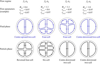
Furthermore, Zhang et al. (Reference Zhang, Nathan, Tian and Chin2021b) revealed that the secondary particle flow structure varies from a reversed four-cell (two centre-downward cells above and two centre-upward cells below) to a six-cell (reversed four-cell above and two centre-downward cells below), and a centre-downward two-cell structure, with the above-mentioned variations in flow parameters. They also identified various combinations of the secondary flow structures of both the fluid and particle phases: the  $f_2$–
 $p_4$ (a two-cell structure for the secondary flow motions of the fluid phase and a four-cell structure for that of the particle phase; the same conventions apply hereafter),
 $f_4$–
 $p_6$,
 $f_4$–
 $p_2$ and
 $f_2$–
 $p_2$ regimes, as illustrated in figure 1. Each of these represent different secondary flow structures of both phases and occurs for different characteristics of the flow parameters. However, the governing mechanisms for driving such different secondary flow motions, particularly for the pair of centre-downward secondary fluid flow cells, and various secondary particle flow structures, have not been reported previously.
In summary, for horizontal particle-laden pipe flows, the secondary fluid flow of the second kind that results from an inhomogeneous particle distribution has been observed and confirmed in terms of the anisotropy of the Reynolds stresses in the literature. In contrast, the secondary fluid flow of the first kind has only been hypothesised to occur where the particle mass loading is sufficiently high, i.e. to be dominated by the fluid–particle interaction force exerted on the fluid, while the anisotropy of Reynolds stress is negligible. However, the direct evidence supporting this hypothesis is missing. Moreover, the fact that both the anisotropy of Reynolds stresses and the fluid–particle interaction force can be non-zero implies that conditions may arise in which a secondary fluid flow could be of both the first and second kinds. This, in turn, suggests that this classification may be incomplete and that an assessment should be performed based on instantaneous forces (e.g. the pressure gradient force and fluid–particle interaction force) in addition to the Reynolds stresses. Since such analyses are not available, the aims of the present numerical work are: (1) to characterise completely the class(es) of secondary flows in horizontal particle-laden pipe flows; and (2) to advance understanding of the generation of such secondary flows from an analysis of the forces acting on both the fluid and particle phases. Here, we stress that although our previous studies have identified various flow regimes and their characteristics, including the secondary flow patterns, no detailed explanation was given for the mechanism for the secondary flow phenomenon, whereas the present study focuses on the dominant mechanisms of secondary flows.
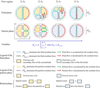
The paper is organised as follows. Section 2 describes the governing equations, applied models, numerical configurations and data post-processing in the present work. In § 3, the secondary fluid flows are identified, and the forces exerted on both the fluid and particle phases are presented. Section 4 summarises the mechanisms with which the secondary flows of both phases are generated, using sketches. Finally, conclusions are drawn in § 5.
Illustration of the various regimes of secondary flow structures of both the fluid and particle phases identified previously Zhang et al. (Reference Zhang, Nathan, Tian and Chin2021b). Here, a subscript following the symbols f and p represents the number of cells in the fluid and particle phases, respectively. Also shown are typical values of mass loading and CORs that generate these regimes.

2. Numerical method
2.1. Governing equations
A direct numerical simulations (DNS) method with four-way coupling Lagrangian particle tracking in an open source framework (OpenFOAM $^\circledR$) was employed to solve the N–S equations and those of particle motions, following the numerical framework of Zhang et al. (Reference Zhang, Nathan, Tian and Chin2021a,Reference Zhang, Nathan, Tian and Chinb). The motion of an incompressible fluid (gas) phase in a horizontal circular pipe is governed by the volume-averaged continuity and N–S equations, given by
 $$\begin{gather} \frac{\partial \alpha^f }{\partial t}+\boldsymbol{\nabla} \boldsymbol{\cdot} (\alpha^f \boldsymbol{u}^f)=0, \end{gather}$$
 $$\begin{gather}\frac{\partial (\alpha^f \boldsymbol{u}^f)}{\partial t}+\boldsymbol{\nabla} \boldsymbol{\cdot} (\alpha^f \boldsymbol{u}^f\boldsymbol{u}^f)={-}\frac{1}{\rho^f}\,\boldsymbol{\nabla} p+\boldsymbol{\nabla} \boldsymbol{\cdot} (\alpha^f \boldsymbol{\varepsilon})+\alpha^f {\boldsymbol{g}}-\boldsymbol{S_p}, \end{gather}$$
where  $\boldsymbol {u}^f$ and
 $\alpha ^f$ are the velocity vector and volume fraction, respectively, of the fluid phase (with a superscript ‘
 $f$’). Also,
 $p$ denotes the pressure, while
 $\boldsymbol {S}_p$ indicates the particle source term,
 $\boldsymbol {\varepsilon }$ is the viscous stress tensor, and
 $\boldsymbol {g}$ is the gravitational acceleration vector. The fluid viscous stress tensor
 $\boldsymbol {\varepsilon }$ is given by
 \begin{equation} \boldsymbol{\varepsilon}=\frac{1}{\rho_f}\left[\left(\lambda_f+ \frac{2}{3}\,\mu_f\right)(\boldsymbol{\nabla} \boldsymbol{\cdot} \boldsymbol{u_f})\delta_K +\mu_f((\boldsymbol{\nabla} \boldsymbol{\cdot} \boldsymbol{u_f})+ (\boldsymbol{\nabla} \boldsymbol{\cdot} \boldsymbol{u_f})^{\rm T})\right], \end{equation}
where  $\lambda _f$ is the fluid bulk viscosity and
 $\delta _K$ is the Kronecker delta. For the present low volume fraction (of the order of
 $10^{-3}$) of particles transported within the incompressible gas, the fluid bulk viscosity
 $\lambda _f$, as well as the effect of mixture viscosity, can be neglected. Furthermore, we note here that the discretisation schemes for these Eulerian governing equations ((2.1) and (2.2)) can be found in the previous numerical work reported by Zhang et al. (Reference Zhang, Nathan, Tian and Chin2021a).
The particle motions are governed by Newton's second law, as follows:
 \begin{equation} m^p_i\,\frac{\mathrm{d}\boldsymbol{u}^p_i}{\mathrm{d}t}= \boldsymbol{f}^p_{D,i}+\boldsymbol{f}^p_{L,i}+ \boldsymbol{f}^p_{G,i}+\boldsymbol{f}^p_{C,iw}+ \sum_{i\neq j}\boldsymbol{f}^p_{C,ij}, \end{equation}
where  $m^p_i$ and
 $\boldsymbol {u}^p_i$ are the mass and the velocity vector for a single particle
 $i$ (with a superscript ‘
 $p$’ indicating the particle phase). Here, the drag force
 $\boldsymbol {f}^p_{D,i}$, lift force
 $\boldsymbol {f}^p_{L,i}$ and gravitational force
 $\boldsymbol {f}^p_{G,i}$ in the negative
 $z$-direction were considered, following the assumptions for particle forces of Zhang et al. (Reference Zhang, Nathan, Tian and Chin2021a). Additionally, the contacting forces of particle
 $i$ with the wall,
 $\boldsymbol {f}^p_{C,iw}$, and with other particle(s)
 $j$,
 $\boldsymbol {f}^p_{C,ij}$, were included and computed using the spring–slider–dashpot model (see Fernandes et al. (Reference Fernandes, Semyonov, Ferrás and Nóbrega2018) for detailed information). The drag force was calculated, depending on the particle volume fraction and the fluid–particle slip velocity, as
 \begin{equation} \boldsymbol{f}^p_{D,i}=\frac{V_i\beta_i}{\alpha^p_i}\, (\boldsymbol{u}^f_i-\boldsymbol{u}^p_i), \end{equation}
where  $V_i$ denotes the volume of a single particle
 $i$, and
 $\boldsymbol {u}^f_i$ indicates the local fluid velocity vector at the
 $i$th particle position. Here,
 $\beta _i$ is an empirical inter-phase momentum exchange coefficient (in units
 $\mathrm {kg}\ \mathrm {m}^{-3}\ \mathrm {s}^{-1}$) computed using the Gidaspow drag model (Gidaspow Reference Gidaspow1994), which combines the empirical correlations presented by Ergun & Orning (Reference Ergun and Orning1949) and Wen & Yu (Reference Wen and Yu1966) for
 $\alpha ^f\leq 0.8$ and
 $\alpha ^f\geq 0.8$, respectively. Also,
 $\alpha ^p_i$ is the local particle volumetric fraction of the computational cell where the particle
 $i$ resides, given by
 \begin{equation} \alpha^p_i=\frac{1}{V_{cell}}\sum _{i=1}^{N^p} V_i, \end{equation}
where  $V_{cell}$ is the volume of the computational cell, and
 $N^p$ is the number of particles found in this cell. Thus the fields of particle and fluid volumetric fractions satisfy
 $\alpha ^p+\alpha ^f=1$. Furthermore, the fluid–particle interaction forces exerted on the local fluid phase (i.e. the source term
 $\boldsymbol {S}_p$ in (2.2)) were computed as the integral of the counteracting forces of the forces exerted by the fluid on the particles (only the drag and lift forces in the present work,
 $\boldsymbol {f}^f_{D,i}=-\boldsymbol {f}^p_{D,i}$,
 $\boldsymbol {f}^f_{L,i}=-\boldsymbol {f}^p_{L,i}$) per unit of volume, given by
 \begin{equation} \boldsymbol{S}_p = \frac{\displaystyle \sum _{i=1}^{N^p}(\boldsymbol{f}^f_{D,i} +\boldsymbol{f}^f_{L,i})}{\rho^f V_{cell}}. \end{equation}
We note here that the term  $\boldsymbol {S}_{p,y-z}$ in (1.2) is the projection of the vector
 $\boldsymbol {S}_p$ onto the two-dimensional pipe cross-section.
Moreover, in (2.4), the lift force was calculated depending on the cross-product of the fluid–particle slip velocity and fluid vorticity, as follows:
 \begin{equation} \boldsymbol{f}^p_{L,i} = C_L\boldsymbol{\cdot} \rho^f\boldsymbol{\cdot} V_i \boldsymbol{\cdot}(\boldsymbol{u}^f_i-\boldsymbol{u}^p_i) \times \omega_i, \end{equation}
where  $\omega _i$ is the fluid vorticity (
 $\omega = \boldsymbol {\nabla } \times \boldsymbol {u}^f$) at the
 $i$th particle position. Here,
 $C_L$ is the lift coefficient in terms of the particle Reynolds number
 $Re^p=\rho ^f\,| \boldsymbol {u}^p-\boldsymbol {u}^f |\,d/\mu$ and the vorticity Reynolds number
 $Re_\omega =\rho ^f\,| \boldsymbol {\nabla } \times \boldsymbol {u}^f |\,{d}^2 /\mu$, where
 $d$ is the particle diameter. The Saffman lift force model, corrected by Mei (Reference Mei1992) and Mei & Klausner (Reference Mei and Klausner1994) for moderate particle Reynolds numbers, was employed in the present study to evaluate the effect of particle motions near to the wall where velocity gradients are high.
2.2. Numerical configurations
The configuration of simulations followed the previous numerical work by Zhang et al. (Reference Zhang, Nathan, Tian and Chin2021a,Reference Zhang, Nathan, Tian and Chinb). The fluid bulk Reynolds number was  $Re^f_b=\rho ^f U^f_bD/\mu = 20 000$ based on the fluid bulk velocity
 $U^f_b$ and pipe diameter
 $D$, while the shear Reynolds number was
 $Re^f_\tau = 570$. The particle-to-gas density ratio was fixed at
 $\rho _r = \rho ^p / \rho ^f =1000$. A constant Stokes number
 $Sk=\rho ^p{d}^2U^f_b/(18\mu D) = 11.2$ and a constant Froude number
 $Fr=U^f_b/\sqrt {|\boldsymbol {g}| D} = 17$ were used, which are the moderate values employed by Zhang et al. (Reference Zhang, Nathan, Tian and Chin2021a), who assessed conditions in the ranges
 $1.4\leq Sk \leq 40.5$ and
 $8.5 \leq Fr \leq 34$, as well as the sensitivity of the flow behaviour to these parameters. Also, note that the Stokes number is associated with the ratio of the particle viscous relaxation time to the flow-through time (where one flow-through time refers to the fluid passing through the computational domain with the bulk velocity once). The CORs of particle–wall and inter-particle collisions in the present work were fixed at
 $e_{p-w}=e_{p-p}=0.97$, while the sensitivity of flow behaviour to both CORs was reported by Zhang et al. (Reference Zhang, Nathan, Tian and Chin2021b). Also, a constant value was used for the coefficient of friction
 $\mu _{fri}=0.1$ (Goldschmidt, Beetstra & Kuipers Reference Goldschmidt, Beetstra and Kuipers2002; Geurts Reference Geurts2010), for both particle–wall and inter-particle collisions in the present flow. The variable controlled in the present work was the mass loading alone, varying from
 $\varPhi _m=0.4$ to
 $0.9$,
 $1.2$ and
 $1.8$ (which corresponds to the volume fraction of the order of
 $10^{-3}$, spanning the transition between the two-way and four-way coupling regimes). It should be noted that the cases with
 $\varPhi _m=0.4$ and
 $1.8$, which we reported previously (Zhang et al. Reference Zhang, Nathan, Tian and Chin2021b) for the flow statistics only, were repeated within a new time window, as described in detail below (producing almost the same statistical results because of the full development of the flow), and were post-processed for force analyses so that the current numerical results are completely new. Moreover, the cases
 $\varPhi _m=0.9$ and
 $1.2$ were added to obtain additional flow regimes via such a single variable parameter. Furthermore, we note here that the mass loading was prescribed based on the assumption that the bulk particle velocity equals the bulk fluid velocity. Hence the actual values of the mass loading ratio could vary, while the particle volume fraction remains constant during the simulation.
The simulation was performed for a streamwise-periodic pipe of length  $x=6D$. The periodic condition was applied to both the fluid and particle phases, i.e. particles moving outside the domain in the streamwise direction were reintroduced via periodicity. For the Eulerian fluid phase, a momentum source was included in the pressure gradient term
 $\boldsymbol {\nabla } p$, in (2.2), whose streamwise component,
 $(\boldsymbol {\nabla } p)_x$, was adjusted implicitly in the simulation to drive the flow with a constant
 $U^f_b$. An O-type mesh layout was employed using
 $11.5$ million grid points, with the near-wall grids being refined to resolve the turbulent boundary layer. The dimensionless grid size in the streamwise direction was
 $\Delta x^+=19.9$, while in the azimuthal direction near to the pipe wall it was
 $\Delta r\theta ^+|_{wall}=12.4$, in the radial direction near to the pipe wall it was
 $\Delta y^+|_{wall}=0.8$, and in the pipe centre it was
 $\Delta y^+|_{centre}=8.0$. Here, the superscript ‘+’ indicates the normalised value in the wall units, e.g.
 $\Delta x^+ = (\Delta x \boldsymbol {\cdot } u_\tau )/\nu$, where the inner variables
 $u_\tau$ and
 $\nu$ are the shear velocity and kinematic viscosity. The present grid resolution is sufficient to resolve the Kolmogorov scale and ensure that the fluid statistics are independent of it. Note that, as reported by Burton & Eaton (Reference Burton and Eaton2005) and Vreman (Reference Vreman2015), and as clarified in our previous work (Zhang et al. Reference Zhang, Nathan, Tian and Chin2021b), though the particle size in wall units is
 $d^+ = 3.5$ (equivalent to four wall-normal grid dimensions near to the pipe wall), it affects only the turbulence intensity but not the mean fluid velocity, including the secondary flow patterns. As suggested by Balachandar (Reference Balachandar2009) and Balachandar & Eaton (Reference Balachandar and Eaton2010), for such large particles with a size of the order or larger than the Kolmogorov scale, a separate deterministic and stochastic component needs to be included in the drag and lift forces to model the effects of turbulence on inter-phase coupling accurately. However, the best way to incorporate these effects remains an open research question.
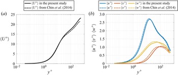
For the Lagrangian part, the particles were initially released from randomly distributed locations over the entire domain, with an initial velocity equal to the local fluid velocity. The calculation of the contact force during collisions was given according to the positions and overlapping rates between a particle and the wall, or between two colliding particles, with the new velocity and acceleration of particle(s) being updated for every Lagrangian sub-iteration. This sub-iteration is five times smaller than the simulation time step, and much smaller than the particle response time, which enables the capture of the physics of particle collisions. We note here that the validation of this numerical model for particle-laden flows can be found in the previous study (Zhang et al. Reference Zhang, Nathan, Tian and Chin2021a), while its validation for turbulence statistics in single-phase flows is in Appendix A.
2.3. Process of force statistics
The gravitational term in the momentum equation of the fluid phase,  $\alpha ^f\boldsymbol {g}$, is negligible for the fluid (gas) phase (see (2.2)). Therefore, the sum of the pressure gradient term
 $-({1}/{\rho ^f})\,\boldsymbol {\nabla } p$, the viscous stress tensor term
 $\boldsymbol {\nabla }(\alpha ^f \boldsymbol {\varepsilon })$ and the particle source term
 $-\boldsymbol {S}_p$ equals the material derivative of the fluid velocity,
 ${\mathrm {D}\boldsymbol {u}^f}/{\mathrm {D}t} = {\partial (\alpha ^f \boldsymbol {u}^f)}/{\partial t}+\boldsymbol {\nabla } \boldsymbol {\cdot } (\alpha ^f \boldsymbol {u}^f\boldsymbol {u}^f)$, which represents the total acceleration of fluid particles for each numerical time step. In view of this, we calculated all four terms separately in the simulation, to identify the contribution of each fluid force to the secondary fluid flow motions.
Also, in the momentum equation of the particle phase (see (2.4)), we calculated the drag force  $\boldsymbol {f}^p_D$, lift force
 $\boldsymbol {f}^p_L$, particle–wall contacting force
 $\boldsymbol {f}^p_{C,W}$ and particle resultant force
 $m^p({\mathrm {d}\boldsymbol {u}^p}/{\mathrm {d}t})$, separately, to identify the contribution of each of these forces to the particle motions. Hence it is clear that the sum of the former three, combined with the gravitational force
 $\boldsymbol {f}^p_G$, equals the latter. Note that the statistics of the particle phase introduced here without a subscript ‘
 $i$’ are the locally averaged values, thus the inter-particle contacting force is zero as they were cancelled out by each other locally.
The normalised pressure gradient force  $\boldsymbol {F}^f_{\nabla p}$, viscous force
 $\boldsymbol {F}^f_{\varepsilon }$, fluid–particle interaction force (via drag and lift alone)
 $\boldsymbol {F}^f_{S,p}$ and resultant force
 $\boldsymbol {F}^f_{tot}$ exerted on the fluid phase, together with the normalised drag force
 $\boldsymbol {F}^p_{D}$, lift force
 $\boldsymbol {F}^p_{L}$, particle–wall contacting force
 $\boldsymbol {F}^p_{C,W}$, gravitational force
 $\boldsymbol {F}^p_{G}$ and resultant force
 $\boldsymbol {F}^p_{tot}$ exerted on the particle phase, were calculated by dividing their locally averaged values normalised by the magnitude of the gravitational force in the flow system, as follows:
 \begin{align} &\boldsymbol{F}^f_{\nabla p} = \frac{m^f_i\left(-\dfrac{1}{\rho^f}\, \boldsymbol{\nabla} p \right)}{m^f_i|\boldsymbol{g}|},\quad \boldsymbol{F}^f_{\varepsilon} = \frac{m^f_i [\boldsymbol{\nabla}\boldsymbol{\cdot} (\alpha^f \boldsymbol{\varepsilon})]}{m^f_i|\boldsymbol{g}|} ,\nonumber \\ &\boldsymbol{F}^f_{S,p} = \frac{m^f_i(-\boldsymbol{S_p})}{m^f_i| \boldsymbol{g}|},\quad \boldsymbol{F}^f_{tot} = \frac{m^f_i \left(\dfrac{\mathrm{D}\boldsymbol{u}^f}{\mathrm{D}t}\right)}{m^f_i| \boldsymbol{g}|}, \end{align}
and
 \begin{align} &\boldsymbol{F}^p_{D} = \frac{\boldsymbol{f}^p_D}{m^p_i |\boldsymbol{g}|},\quad \boldsymbol{F}^p_{L} = \frac{\boldsymbol{f}^p_L}{m^p_i|\boldsymbol{g}|},\quad \boldsymbol{F}^p_{C,W} = \frac{\boldsymbol{f}^p_{C,W}}{m^p_i| \boldsymbol{g}|},\nonumber\\ &\boldsymbol{F}^p_{G} =\frac{\boldsymbol{f}^p_G}{m^p_i|\boldsymbol{g}|}=(0,0,-1), \quad \boldsymbol{F}^p_{tot} = \frac{m^p_i\left(\dfrac{\mathrm{d} \boldsymbol{u}^p}{\mathrm{d}t}\right)}{m^p_i|\boldsymbol{g}|}, \end{align}
where  $m^f_i$ and
 $m^p_i$ represent the masses of the virtual fluid particle and the solid particle, respectively. Also, these statistics satisfy the relationships
 \begin{equation} \boldsymbol{F}^f_{\nabla p} + \boldsymbol{F}^f_{\varepsilon} + \boldsymbol{F}^f_{S,p} = \boldsymbol{F}^f_{tot} \end{equation}
and
 \begin{equation} \boldsymbol{F}^p_{D} + \boldsymbol{F}^p_{L} + \boldsymbol{F}^p_{C,W} + \boldsymbol{F}^p_{G} = \boldsymbol{F}^p_{tot}. \end{equation}
The cross-sectional distributions of these force statistics are presented in § 3 by averaging them over time and space in the streamwise direction of the entire domain (indicated by the brackets  $\langle \ \rangle$) for
 $314$ flow-through times after the flow reached a statistically stationary state.
3. Results
3.1. Secondary flow structures and flow statistics
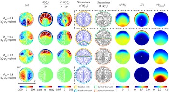
Figure 2 presents the fluid streamwise vorticity  $\langle \omega ^+_{x} \rangle$ together with the gradients of radial and azimuthal Reynolds stresses,
 ${\partial \langle \tau _{rr}^+ \rangle }/{\partial r}$ and
 $({D}/{r})({\partial \langle \tau _{\theta \theta }^+ \rangle }/{\partial \theta })$, for the four flow regimes
 $f_2$–
 $p_4$,
 $f_4$–
 $p_6$,
 $f_4$–
 $p_2$ and
 $f_2$–
 $p_2$, while varying only the mass loading from
 $\varPhi _m=0.4$ to
 $\varPhi _m=1.8$. Also shown are the corresponding secondary flows of the fluid and particle phases, i.e. the streamlines of
 $\langle \boldsymbol {u}^{f}_{y-z}\rangle$ and
 $\langle \boldsymbol {u}^{p}_{y-z}\rangle$, respectively, together with the mean static pressure
 $\langle P/P_0 \rangle$, and the particle local mass loading
 $\langle \varPhi _{m,loc} \rangle$, for reference. It should be noted that although we have previously published similar data (indicated by the black dot-dashed boxes in the last five columns) for
 $\varPhi _m=0.4$ and
 $1.8$ (Zhang et al. Reference Zhang, Nathan, Tian and Chin2021b), the current dataset is completely new as it not only includes new cases (
 $\varPhi _m=0.9$ and
 $1.2$, designed to obtain the four flow regimes in a single variable
 $\varPhi _m$) but also fully repeats these previous simulations within a new time window. Importantly, negligible differences for these statistics in the black dot-dashed boxes between the present study and the previous work can be observed, confirming the convergence and repeatability of the simulation results.
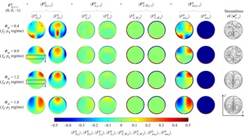
Cross-sectional views of the flow patterns and key properties for each of the four flow regimes obtained by varying mass loading alone, from  $\varPhi _m=0.4$ to
 $\varPhi _m=1.8$. The columns from left to right are: fluid streamwise vorticity; gradient of the radial Reynolds stress; gradient of the azimuthal Reynolds stress; secondary fluid flow motions; secondary particle flow motions; static pressure; turbulence kinetic energy; local mass loading. Here, the brackets
 $\langle \rangle$ indicate the average over time and space (in the streamwise direction of the entire domain), while the superscript ‘+’ indicates the normalised value in wall units. The sparse white streamlines also shown in the first three columns are the secondary fluid flow motions for reference, while the purple arrows in the second and third columns indicate the directions of the gradients of the Reynolds stresses. The black dot-dashed lines in the first and last rows indicate the reproduced results, similar to the study published previously (Zhang et al. Reference Zhang, Nathan, Tian and Chin2021b) for the same cases. Other conditions are
 $Sk=11.2$,
 $Fr=17$,
 $e_{p-w}=e_{p-p}=0.97$; the direction of gravity is downwards.

For convenience, for the secondary fluid flow structure in the fourth column of figure 2, we term the pair of centre-upward cells of the secondary fluid flow structure (anticlockwise on the left and clockwise on the right; see the regions surrounded by the yellow dashed lines) ‘ $fluid$-
 $up$-
 $cells$’. These cells exhibit similar characteristics and have been proposed to be categorised into a secondary flow of the second kind that is induced by the anisotropy of turbulence (Zhang et al. Reference Zhang, Nathan, Tian and Chin2021b). In contrast, we term the pair of centre-downward cells (the contrary two cells; see the regions surrounded by the blue dashed lines) ‘
 $fluid$-
 $down$-
 $cells$’. These cells also exhibit similar characteristics (different from the above) and have been hypothesised to be categorised into a secondary flow of the first kind that is caused by the fluid–particle interaction forces (Zhang et al. Reference Zhang, Nathan, Tian and Chin2021b). Similarly, for the secondary particle flow structure in the fifth column, we term the reversed four-cell structure (see the regions surrounded by the green dotted lines) ‘
 $particle$-
 $four$-
 $cells$’, while the pair of centre-downward cells (see the regions surrounded by the red dotted lines) are termed ‘
 $particle$-
 $down$-
 $cells$’.
From the first column in figure 2, it can be seen that the absolute value of  $\langle \omega ^+_{x} \rangle$, which is a measure of the strength of the secondary fluid flow motions, decreases in the
 $fluid$-
 $up$-
 $cells$ region with an increase in mass loading
 $\varPhi _m$. For example, the absolute peak value
 $|\langle \omega ^+_{x} \rangle |_{max} \geq 200$, which occurs in the lower half of the pipe for the
 $f_2$–
 $p_4$ regime, decreases to
 $|\langle \omega ^+_{x} \rangle |_{max} \approx 120$ and shifts to the upper half of the pipe for the
 $f_4$–
 $p_2$ regime. This coincides with a shrinkage of the
 $fluid$-
 $up$-
 $cells$, in which turbulence persists. In contrast, the strength of the secondary fluid flow motions in the
 $fluid$-
 $down$-
 $cells$ region increases from
 $|\langle \omega ^+_{x} \rangle |_{max} \approx 0$ to
 $120$ with increase in
 $\varPhi _m$ from
 $0.9$ to
 $1.8$, and hence the transition from the
 $f_4$–
 $p_6$ regime to the
 $f_2$–
 $p_2$ regime. This coincides with an enlargement of the
 $fluid$-
 $down$-
 $cells$, in which the turbulence has been attenuated greatly by the increased local particle mass loading
 $\varPhi _{m,loc}$ (see the last column). Also, note that the sign of
 $\langle \omega ^+_{x} \rangle$ is opposite in the
 $fluid$-
 $up$-
 $cells$ and
 $fluid$-
 $down$-
 $cells$ regions, which means that their secondary fluid flows are in opposite directions. Overall, the shrunken
 $fluid$-
 $up$-
 $cells$ with their weakened secondary flows and the enlarged
 $fluid$-
 $down$-
 $cells$ with their enhanced, reversed secondary flows coincide with each other. Both regions are associated with the increase in
 $\varPhi _m$, particularly the increase in
 $\varPhi _{m,loc}$ in the lower half of the pipe.
The second and third columns of figure 2 present the radial and azimuthal gradients of the Reynolds stresses,  ${\partial \langle \tau _{rr}^+ \rangle }/{\partial r}$ and
 $({D}/{r})({\partial \langle \tau _{\theta \theta }^+ \rangle }/{\partial \theta })$. These are the dominant terms of
 $(\boldsymbol {\nabla } \boldsymbol {\cdot } \tilde {\boldsymbol {\tau }}_{y-z})_r$ and
 $(\boldsymbol {\nabla } \boldsymbol {\cdot } \tilde {\boldsymbol {\tau }}_{y-z})_\theta$, respectively (Belt et al. Reference Belt, Daalmans and Portela2012; Vollestad et al. Reference Vollestad, Angheluta and Jensen2020), which are the radial and azimuthal components of the divergence of the Reynolds stress tensor (i.e.
 $\boldsymbol {\nabla } \boldsymbol {\cdot } \tilde {\boldsymbol {\tau }}_{y-z}$ in (1.1)). It can be observed that the
 $fluid$-
 $up$-
 $cells$ occur where
 ${\partial \langle \tau _{rr}^+ \rangle }/{\partial r} \neq 0$ and
 $({D}/{r})({\partial \langle \tau _{\theta \theta }^+ \rangle }/{\partial \theta }) \neq 0$ (i.e.
 $\boldsymbol {\nabla } \times (\boldsymbol {\nabla } \boldsymbol {\cdot } \tilde {\boldsymbol {\tau }}_{y-z}) \neq 0$). Also, the directions of the gradients of the Reynolds stresses (see the purple arrows) are consistent with the secondary flow directions of the
 $fluid$-
 $up$-
 $cells$. On the other hand, the particle local mass loading,
 $\varPhi _{m,loc}$, is relatively low in such cells (see the last column), corresponding to a relatively small fluid–particle interaction force term
 $\boldsymbol {\nabla } \times \boldsymbol {S}_{p,y-z,{0}}$, in (1.1). In particular,
 $\varPhi _{m,loc}$ is approximately zero in the top region of such cells (near to the top wall of the pipe), which means that
 $\boldsymbol {\nabla } \times \boldsymbol {S}_{p,y-z,{0}} \approx 0$. Hence the current results support the inference that the secondary fluid flows in the
 $fluid$-
 $up$-
 $cells$ are associated primarily with the anisotropy of the Reynolds stresses, i.e. secondary flows of the second kind. Additionally, the anisotropy of the Reynolds stresses is a primary driver only where the local mass loading is sufficiently low.
In contrast, the values of both  ${\partial \langle \tau _{rr}^+ \rangle }/{\partial r}$ and
 $({D}/{r})({\partial \langle \tau _{\theta \theta }^+ \rangle }/{\partial \theta })$ are approximately equal to zero (i.e.
 $\boldsymbol {\nabla } \times (\boldsymbol {\nabla } \boldsymbol {\cdot } \tilde {\boldsymbol {\tau }}_{y-z})\approx 0$) in the
 $fluid$-
 $down$-
 $cells$ region, which means that the secondary fluid flows in such cells are not associated with the anisotropy of the Reynolds stresses. Instead, it is inferred that such secondary flows are attributed to a non-zero fluid–particle interaction force term,
 $\boldsymbol {\nabla } \times \boldsymbol {S}_{p,y-z,{0}} \neq 0$, from the necessary and sufficient conditions for the presence of secondary flows (see (1.1)). Also, the relatively high values of
 $\varPhi _{m,loc}$ in such cells are supporting evidence for this inference. However, it is challenging to isolate the component,
 $\boldsymbol {S}_{p,y-z,{0}}$, which is independent of the secondary flow velocity, from the fluid–particle interaction force term
 $\boldsymbol {S}_{p,y-z}$ (in (1.2) and (2.2)), as mentioned in § 1. Therefore, the hypothesis that secondary fluid flows in the
 $fluid$-
 $down$-
 $cells$ are caused by the fluid–particle interaction forces exerted on the fluid, i.e. secondary flows of the first kind, still cannot be confirmed.
However, from the gradients of the Reynolds stresses (the second and third columns of figure 2) for the  $f_4$–
 $p_6$ and
 $f_4$–
 $p_2$ regimes, it is reasonable to suppose that both
 $\boldsymbol {\nabla } \times (\boldsymbol {\nabla } \boldsymbol {\cdot } \tilde {\boldsymbol {\tau }}_{y-z}) \neq 0$ and
 $\boldsymbol {\nabla } \times \boldsymbol {S}_{p,y-z,{0}} \neq 0$ are true in the transition region between the
 $fluid$-
 $up$-
 $cells$ and
 $fluid$-
 $down$-
 $cells$. This supposition is made because the variations in the distributions of both the Reynolds stress gradients and the particle local mass loading (in the last column) are continuous, i.e. they are continuous functions of spatial locations within the pipe domain. That is, the majority of the
 $fluid$-
 $up$-
 $cells$ and
 $fluid$-
 $down$-
 $cells$ could be classified as the first and second kinds of the secondary flow, respectively, while the transition region between them could be of both kinds.
3.2. Fluid force analysis
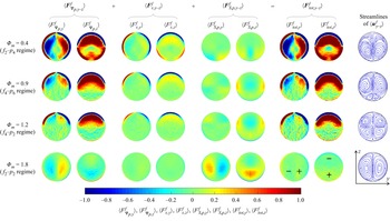
Figure 3 presents the mean cross-sectional distributions of the normalised pressure gradient force  $\langle \boldsymbol {F}^f_{\nabla p,{y-z}} \rangle$, viscous force
 $\langle \boldsymbol {F}^f_{\varepsilon,{y-z}} \rangle$, fluid–particle interaction force
 $\langle \boldsymbol {F}^f_{S,p,{y-z}} \rangle$ and resultant force
 $\langle \boldsymbol {F}^f_{tot,{y-z}} \rangle$ exerted on the fluid, decomposed into the transverse (
 $y$-axis) and vertical (
 $z$-axis) components. The figure is presented to span the four flow regimes as a function of the single variable of mass loading varying from
 $\varPhi _m=0.4$ to
 $\varPhi _m=1.8$. As mentioned in § 2.3, the sum of the former three forces equals the latter resultant force for all cases.
Colour maps of the gravity-normalised, mean cross-sectional forces exerted on the fluid phase: the pressure gradient force  $\langle \boldsymbol {F}^f_{\nabla p,{y-z}} \rangle$, viscous force
 $\langle \boldsymbol {F}^f_{\varepsilon,{y-z}} \rangle$ and fluid–particle interaction force
 $\langle \boldsymbol {F}^f_{S,p,{y-z}} \rangle$, together with the resultant force
 $\langle \boldsymbol {F}^f_{tot,{y-z}} \rangle$, which equals the sum of the first three. All the statistics are decomposed into the transverse (
 $y$-axis, positive indicates rightwards) and vertical (
 $z$-axis, positive indicates upwards) components. Other flow conditions are as per figure 2. Also shown are the secondary fluid flow structures in the last column, for reference.

From the first two columns in figure 3, it can be seen that the increase in mass loading, and hence the transition from the  $f_2$–
 $p_4$ regime to the
 $f_2$–
 $p_2$ regime, is associated with a reduction in both the magnitude and extent of the relatively high pressure gradient forces (
 $| \langle \boldsymbol {F}^f_{\nabla p,y-z} \rangle | \sim {O}(1)$). This trend coincides with those reported above for the streamwise vorticity
 $\langle \omega ^+_{x} \rangle$, and the extent of
 $fluid$-
 $up$-
 $cells$ (see § 3.1). In other words, the magnitudes of the components of
 $\langle \boldsymbol {F}^f_{\nabla p, y-z} \rangle$ in the
 $fluid$-
 $up$-
 $cells$ region are relatively high; in particular,
 $|\langle F^f_{\nabla p,y} \rangle | \gg 1$ and
 $|\langle F^f_{\nabla p,z} \rangle | \gg 1$ near to the pipe wall. In contrast, these magnitudes in the
 $fluid$-
 $down$-
 $cells$ region are relatively low. They increase from nearly zero to
 $|\langle F^f_{\nabla p,y} \rangle | \approx 0.3$ and
 $|\langle F^f_{\nabla p,z} \rangle | \approx 0.3$ with the increase in mass loading, and hence the transition of regimes mentioned above. Also, this trend coincides with the variation in
 $\langle \omega ^+_{x} \rangle$ within the
 $fluid$-
 $down$-
 $cells$ region (see § 3.1).
The above-mentioned variations of the distribution of  $\langle \boldsymbol {F}^f_{\nabla p,y-z} \rangle$ in figure 3 are attributed to the changes in static pressure difference in different flow regimes (see the third column from last in figure 2). The higher concentration of particles in the region near the bottom of the pipe, due to gravitational settling, decelerates the fluid there, which results in a higher pressure than that in the top region of the pipe. This explains the secondary flow direction in the
 $fluid$-
 $up$-
 $cells$. However, a further increase in the particle mass loading leads to a local value
 $\langle \varPhi _{m,loc}\rangle \geq 1.5$ (see the last column of figure 2), which attenuates the local turbulence significantly, resulting in a lower pressure difference, thus explaining the weak pressure gradient force in the
 $fluid$-
 $down$-
 $cells$ for this case. We note here that where the value of
 $\langle \varPhi _{m,loc}\rangle \geq 1.5$ extends to the core region of the pipe, any large-scale turbulent vortices are quickly dissipated or never generated, followed by secondary dissipation of the small-scale vortices. This case corresponds to strongly attenuated turbulence, resulting in low pressure gradients throughout the domain for the
 $f_2$–
 $p_2$ regime (see the second and third columns from last in figure 2). The above-mentioned interpretation for the distribution of pressure difference (i.e. the pressure gradient force) in each flow regime is consistent with the previous work by Zhang et al. (Reference Zhang, Nathan, Tian and Chin2021b).
The distribution of viscous force  $\langle \boldsymbol {F}^f_{\varepsilon,{y-z}} \rangle$ in the third and fourth columns of figure 3 exhibits the same trend as
 $\langle \boldsymbol {F}^f_{\nabla p,y-z} \rangle$ in the near-wall region for various flow regimes. Its magnitude is considerable in the
 $fluid$-
 $up$-
 $cells$ because the turbulence persists, and the turbulent shear stresses are relatively strong. In contrast, it is negligible in the
 $fluid$-
 $down$-
 $cells$ because the turbulence is attenuated greatly, so that the turbulent shear stresses are weak. Furthermore, the contribution of
 $\langle \boldsymbol {F}^f_{\varepsilon,{y-z}} \rangle$ is considerable in the viscous and buffer layers of the turbulent flow, particularly close to the wall, while it can be neglected in the outer layer because the turbulent shear stresses are dominant (Pope Reference Pope2000). The position of the boundary between the buffer and outer layers in wall units is
 $y^+\approx 30$, corresponding to the radial distance normalised by the pipe diameter
 $r/D \approx 0.47$ for the present pipe flows. That is, the
 $\langle \boldsymbol {F}^f_{\varepsilon,{y-z}} \rangle$ term can be neglected, and the relationship
 $\langle \boldsymbol {F}^f_{\nabla p,y-z} \rangle + \langle \boldsymbol {F}^f_{S,p,{y-z}} \rangle = \langle \boldsymbol {F}^f_{tot,{y-z}} \rangle$ is satisfied in the outer region (
 $r/D \leq 0.47$) for the present cases.
The value of  $\langle \boldsymbol {F}^f_{S,p,{y-z}} \rangle$ (fifth and sixth columns in figure 3), which is the normalised local integral of the drag and lift forces exerted by particles on the fluid (see (2.7)), is progressively more significant in both the
 $y$- and
 $z$-directions with the increase in
 $\varPhi _m$, and hence the transition from the
 $f_2$–
 $p_4$ regime to the
 $f_2$–
 $p_2$ regime. Given the negligible
 $\langle \boldsymbol {F}^f_{\varepsilon,{y-z}} \rangle$ term in the outer region of the flow mentioned above, the magnitude of
 $\langle \boldsymbol {F}^f_{S,p,{y-z}} \rangle$ is much smaller than that of
 $\langle \boldsymbol {F}^f_{\nabla p,y-z} \rangle$ in the
 $fluid$-
 $up$-
 $cells$ region. That is, the distribution of the resultant force on the fluid,
 $\langle \boldsymbol {F}^f_{tot,{y-z}} \rangle$ (the second and third columns from last in figure 3), is dominated by that of the pressure force
 $\langle \boldsymbol {F}^f_{\nabla p,y-z} \rangle$. In contrast, in the
 $fluid$-
 $down$-
 $cells$ region, the magnitude of
 $\langle \boldsymbol {F}^f_{S,p,{y-z}} \rangle$ is comparable with that of
 $\langle \boldsymbol {F}^f_{\nabla p,y-z} \rangle$, but both forces are opposite in direction. These two forces result in a low resultant force
 $\langle \boldsymbol {F}^f_{tot,{y-z}} \rangle$ there. This can be seen most clearly for the
 $f_2$–
 $p_2$ regime. These variations in
 $\langle \boldsymbol {F}^f_{S,p,{y-z}} \rangle$ are attributed both to the increased particle number with the increase in mass loading and to the changes in the distributions of the counteracting forces of the fluid–particle interaction forces (
 $\boldsymbol {f}^p_{D,i,{y-z}} = -\boldsymbol {f}^f_{D,i,{y-z}}$ and
 $\boldsymbol {f}^p_{L,i,{y-z}} = -\boldsymbol {f}^f_{L,i,{y-z}}$), which are discussed in § 3.3.
The distribution of  $\langle \boldsymbol {F}^f_{tot,{y-z}} \rangle$, shown in the second and third columns from last in figure 3, provides explanations for the direction of the secondary flow. We first note that the magnitude of
 $\langle \boldsymbol {F}^f_{tot,{y-z}} \rangle$ in the
 $fluid$-
 $up$-
 $cells$ is high and dominated by
 $\langle \boldsymbol {F}^f_{\nabla p,y-z} \rangle$. These magnitudes are high because turbulence in such cells persists, thus the flows in the cross-section are strong. In particular, the directions of
 $\langle \boldsymbol {F}^f_{tot,{y-z}} \rangle$ and
 $\langle \boldsymbol {F}^f_{\nabla p,y-z} \rangle$ are towards the pipe core in the region near the pipe wall because the no-slip pipe wall acts as a resistance to the flow where turbulence persists through the pressure field. In contrast, such large magnitudes of
 $\langle \boldsymbol {F}^f_{\nabla p,y-z} \rangle$ and
 $\langle \boldsymbol {F}^f_{tot,{y-z}} \rangle$ are almost absent in the
 $fluid$-
 $down$-
 $cells$ region because of the significant attenuation of turbulence (where the flows in the cross-section are weak or absent).
In the inner region of the  $fluid$-
 $up$-
 $cells$, the resultant force
 $\langle \boldsymbol {F}^f_{tot,{y-z}} \rangle$ is mostly upwards, especially around the vertical centreline of the pipe. It is also leftwards or rightwards in the upper section, which drives the upward flow anticlockwise in the left half of the pipe and clockwise in the right. As a result of the resultant force and continuity of the fluid, the fluid flow circulates as a pair of left anticlockwise and right clockwise cells within the cross-section. Moreover, the magnitude and spatial extent of
 $|\langle \boldsymbol {F}^f_{tot,{y-z}} \rangle | \sim {O}(1)$ decrease and shrink to the upper half of the pipe, respectively, with the transition from the
 $f_2$–
 $p_4$ regime to the
 $f_4$–
 $p_2$ regime. These coincide with the decrease in the streamwise vorticity
 $\langle \omega ^+_{x} \rangle$ and the shrinkage of the
 $fluid$-
 $up$-
 $cells$ (see figure 2). Therefore, the secondary flows in the
 $fluid$-
 $up$-
 $cells$ are dominated by, and their strength is positively associated with, the pressure gradient force.
In contrast, in the inner region of the  $fluid$-
 $down$-
 $cells$, the magnitude of the resultant force,
 $| \langle \boldsymbol {F}^f_{tot,{y-z}} \rangle | \sim {O}(0.1)$, is much weaker than in the
 $fluid$-
 $up$-
 $cells$. This is due to the absence of a strong pressure gradient force
 $\langle \boldsymbol {F}^f_{\nabla p,y-z} \rangle$, whose low magnitude is comparable with, and partly counterbalanced by,
 $\langle \boldsymbol {F}^f_{S,p,{y-z}} \rangle$ in the
 $fluid$-
 $down$-
 $cells$. Additionally, the downward flow around the vertical centreline of the pipe is attributed mainly to the downward
 $\langle \boldsymbol {F}^f_{tot,{y-z}} \rangle$ in the upper section, while it is decelerated in the lower section by the upward
 $\langle \boldsymbol {F}^f_{tot,{y-z}} \rangle$. The downward resultant force is dominated by
 $\langle \boldsymbol {F}^f_{\nabla p,y-z} \rangle$. In addition, the downward flow is followed by a pair of left clockwise and right anticlockwise circulation cells along the streamlines, which are driven by the leftward and rightward resultant forces on the left and right sides, respectively. The resultant force on both sides is dominated by
 $\langle \boldsymbol {F}^f_{S,p,{y-z}} \rangle$. Therefore, both the pressure gradient force and the fluid–particle interaction force contribute to the secondary flows in the
 $fluid$-
 $down$-
 $cells$.
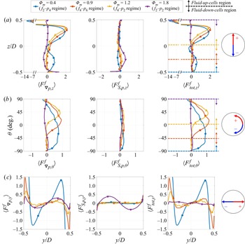
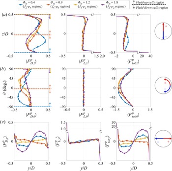
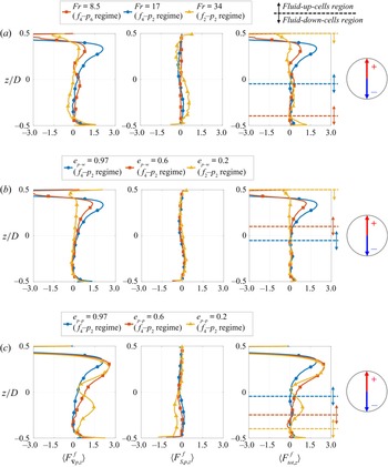
Figures 4(a)–4(c) present the quantitative profiles of the pressure gradient force, fluid–particle interaction force and resultant force exerted on the fluid phase in each of the vertical (with subscript ‘ $z$’), azimuthal (subscript ‘
 $\theta$’) and transverse (subscript ‘
 $y$’) directions. Note that for the azimuthal line, the results in the right half of the pipe alone are shown due to the symmetry (the same goes for the following relevant content). These force components at specific locations are chosen as they represent the forces that contribute to each circulation cell of the secondary fluid flow. It can be seen that the pressure gradient force
 $\langle F^f_{\nabla p} \rangle$ dominates over the fluid–particle interaction force
 $\langle F^f_{S,p} \rangle$, in all three directions within the
 $fluid$-
 $up$-
 $cells$ region. Such a region is
 $z/D \geq -0.5$ &
 $\theta \geq -90^{\circ }$ for the
 $f_2$–
 $p_4$ regime,
 $z/D \geq -0.25$ &
 $\theta \geq -45^{\circ }$ for the
 $f_4$–
 $p_6$ regime, and
 $z/D \geq 0.03$ &
 $\theta \geq 4^{\circ }$ for the
 $f_4$–
 $p_2$ regime (shown as the regions above the dashed line with the same colour for each regime). In contrast, both forces in all three directions are comparable with, but opposite in direction to, each other in the
 $fluid$-
 $down$-
 $cells$ region. Such a region is
 $z/D \leq -0.25$ &
 $\theta \leq -45^{\circ }$ for the
 $f_4$–
 $p_6$ regime,
 $z/D \leq 0.03$ &
 $\theta \leq 4^{\circ }$ for the
 $f_4$–
 $p_2$ regime, and
 $z/D \leq 0.5$ &
 $\theta \leq 90^{\circ }$ for the
 $f_2$–
 $p_2$ regime (below the dashed line for each regime).
Profiles for each of the four regimes of the gravity-normalised, mean forces exerted on the fluid phase: the pressure gradient force (left column) and the fluid–particle interaction force (middle column), together with the resultant force (right column), which equals the sum of the first two in the outer region of the pipe flow ( $r/D\leq 0.47$, where the viscous force is negligible). (a) Vertical forces along the vertical centreline (
 $y/D=0$). (b) Azimuthal forces along the azimuthal line at
 $r/D=0.4$ in the right half of the pipe. (c) Transverse forces along the horizontal centreline (
 $z/D=0$; the subplots are placed with rotation). Note that all subplots are plotted in physical directions.

From figure 4(a), it can be seen that in both the  $fluid$-
 $up$-
 $cells$ and
 $fluid$-
 $down$-
 $cells$, the secondary flows of the fluid along the vertical centreline undergo an acceleration followed by a deceleration. For instance, given the upward flow along the vertical centreline in the
 $fluid$-
 $up$-
 $cells$ region for the
 $f_2$–
 $p_4$ regime (above the blue dashed line,
 $z/D\geq -0.5$), the value of
 $\langle F^f_{tot,z} \rangle$ is mostly positive (i.e. upwards and accelerates the flow) at
 $-0.5\leq z/D \leq 0.4$. For the subsequent locations along the centreline, it is negative (i.e. downwards and decelerates the flow) at
 $0.4 \leq z/D \leq 0.5$ (near the top wall) and reaches
 $\langle F^f_{tot,z} \rangle \approx -14$ (indicated by the broken axis). This high value of
 $\langle F^f_{tot,z} \rangle$ acts as a resistance to the flow in the region near to the no-slip wall, as mentioned previously. Also, the acceleration and deceleration on the downward flow in the
 $fluid$-
 $down$-
 $cells$ region can be found clearly for the
 $f_2$–
 $p_2$ regime (below the purple dashed line,
 $z/D\leq 0.5$). The value of
 $\langle F^f_{tot,z} \rangle$ is negative (i.e. downwards and accelerates the flow) in the upper section of the pipe, yet positive (i.e. upwards and decelerates the flow) in the lower section. This variation in the direction of
 $\langle F^f_{tot,z} \rangle$ is consistent with that of
 $\langle F^f_{S,p,z} \rangle$ rather than
 $\langle F^f_{\nabla p,z} \rangle$, which means that the former is dominant.
From figure 4(b), the trend that secondary fluid flows undergo an acceleration followed by a deceleration along an azimuthal line can also be seen. For instance, given the clockwise secondary flow (in the right half of the pipe) in the  $fluid$-
 $up$-
 $cells$ region for the
 $f_2$–
 $p_4$ regime (above the blue dashed line,
 $\theta \geq -90^{\circ }$), such a flow starts from a segment of negative
 $\langle F^f_{tot,\theta } \rangle$ (i.e. clockwise and accelerates the flow) at
 $80^{\circ }\leq \theta \leq 90^{\circ }$. This acceleration is due to the continuity of the fluid when the upward flow reaches the top region of the pipe and is driven by
 $\langle F^f_{\nabla p,\theta } \rangle$. For the subsequent locations along the azimuthal line,
 $\langle F^f_{tot,\theta } \rangle$ is positive (i.e. anticlockwise and decelerates the flow) at
 $-90^{\circ }\leq \theta \leq 80^{\circ }$. This deceleration is also dominated by
 $\langle F^f_{\nabla p,\theta } \rangle$, which stems from the pressure difference within such a region (see figure 2). Similarly, the anticlockwise flow in the
 $fluid$-
 $down$-
 $cells$ region for the
 $f_2$–
 $p_2$ regime (below the purple dashed line,
 $\theta \leq 90^{\circ }$) undergoes an acceleration at
 $-90^{\circ }\leq \theta \leq -30^{\circ }$ and a deceleration at
 $-30^{\circ }\leq \theta \leq -90^{\circ }$. The azimuthal resultant force in the
 $fluid$-
 $down$-
 $cells$ region is mostly dominated by
 $\langle F^f_{\nabla p,\theta } \rangle$, which is slightly higher than, and partly counterbalanced by,
 $\langle F^f_{S,p,\theta } \rangle$. Also, note that the values of
 $\langle F^f_{S,p,\theta } \rangle$ are always positive (i.e. anticlockwise) for all the regimes. This confirms that the fluid flow along an azimuthal line is either in the opposite direction to the particle flow in the
 $fluid$-
 $up$-
 $cells$, or in the same direction with, but driven by, the particle flow in the
 $fluid$-
 $down$-
 $cells$.
Figure 4(c) presents the fluid transverse forces along the horizontal centreline of the pipe, which is found particularly in the lower section of the  $fluid$-
 $up$-
 $cells$ for the
 $f_4$–
 $p_6$ regime (red), or the upper section of the
 $fluid$-
 $down$-
 $cells$ for the
 $f_4$–
 $p_2$ regime (yellow). It can be seen that the resultant forces
 $\langle F^f_{tot,y} \rangle$ of both regimes are dominated by the pressure gradient force
 $\langle F^f_{\nabla p,y} \rangle$. Also, both forces decrease with an increase in mass loading
 $\varPhi _m$ due to the more significant attenuation of turbulence.
In summary, the flow in the  $fluid$-
 $up$-
 $cells$ is dominated by the pressure gradient force alone. In contrast, the flow in the
 $fluid$-
 $down$-
 $cells$ is dominated by the fluid–particle interaction force in the centre-downward segment and around the vertical centreline, while the rest of the flow in the circulation is dominated by the pressure gradient force. Both forces in the
 $fluid$-
 $down$-
 $cells$ region are comparable with each other, but opposite in direction. This summary is presented and discussed in more detail in § 4.
3.3. Particle force analysis
Figure 5 presents the averaged cross-sectional distributions of the drag force  $\langle \boldsymbol {F}^p_{D,{y-z}} \rangle$, lift force
 $\langle \boldsymbol {F}^p_{L,{y-z}} \rangle$, particle–wall contacting force
 $\langle \boldsymbol {F}^p_{C,W,{y-z}} \rangle$ and resultant force
 $\langle \boldsymbol {F}^p_{tot,{y-z}} \rangle$ exerted on the particle phase, decomposed into the transverse (
 $y$-axis) and vertical (
 $z$-axis) components. The figure is presented to span the four flow regimes as a function of the single variable of mass loading varying from
 $\varPhi _m=0.4$ to
 $\varPhi _m=1.8$. As mentioned in § 2.3, the sum of the first three forces combined with the gravitational force
 $\boldsymbol {F}^p_G = (0,0,-1)$ equals the latter resultant force for all the cases. We note here that the particle–wall contacting force is effective only on the pipe wall with a much greater value,
 $|\langle \boldsymbol {F}^p_{C,W,{y-z}} \rangle | \gg 0.5$ (discussed below for figure 6), while the value is zero inside the pipe. Also, the inter-particle contacting forces are cancelled out (i.e. zero) everywhere due to Newton's third law.
Colour maps of the gravity-normalised, mean cross-sectional forces exerted on the particle phase: the drag force  $\langle \boldsymbol {F}^p_{D,{y-z}} \rangle$, lift force
 $\langle \boldsymbol {F}^p_{L,{y-z}} \rangle$ and particle–wall contacting force
 $\langle \boldsymbol {F}^p_{C,W,{y-z}} \rangle$, together with the resultant force
 $\langle \boldsymbol {F}^p_{tot,{y-z}} \rangle$, which equals the sum of the first three combined with the gravitational force
 $\boldsymbol {F}^p_G=(0,0,-1)$. All the statistics are decomposed into the transverse (
 $y$-axis, positive indicates rightwards) and vertical (
 $z$-axis, positive indicates upwards) components. Note that the dashed box ‘
 $A$’ indicates the difference between regimes. Other flow conditions are as per figure 2. Also shown are the secondary particle flow structures in the last column, for reference.

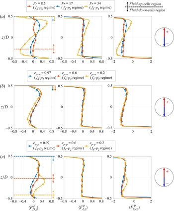
Profiles for each of the four regimes of the gravity-normalised, mean forces exerted on the particle phase: the drag force (left column) and lift force (middle column), together with the resultant force (right column), which equals the sum of the first two combined with the gravitational force  $\boldsymbol {F}^p_G = (0,0,-1)$, in the pipe domain except for the wall (
 $r/D < 0.5$, where there is no particle–wall contacting force). (a) Vertical forces along the vertical centreline (
 $y/D=0$). (b) Azimuthal forces along the azimuthal line at
 $r/D=0.4$ in the right half of the pipe. (c) Transverse forces along the horizontal centreline (
 $z/D=0$, the subplots are placed with rotation). Note that all subplots are plotted in physical directions. Also, the broken axis is shown on one side only of each relevant subplot for conciseness, to indicate the magnitude.

From figure 5, it can be seen that the lift force  $\langle \boldsymbol {F}^p_{L,{y-z}} \rangle$ (third and fourth columns), is strong in the near-wall region only, where the fluid velocity gradient and vorticity are very high and lead to a strong lift force towards the pipe core. In contrast, the magnitude of
 $\langle \boldsymbol {F}^p_{L,{y-z}} \rangle$ is relatively low and plays a less important role than the drag force in the resultant force exerted on the particles away from the pipe wall for all cases. Quantitative comparison can be seen in the following discussion of figure 6. Here, the drag and lift forces exerted by the fluid on particles are the counteracting forces of those exerted by particles on the fluid (
 $\boldsymbol {f}^p_{D} = - \boldsymbol {f}^f_{D}$ and
 $\boldsymbol {f}^p_{L} = - \boldsymbol {f}^f_{L}$). Note that the local integral of these forces on the fluid is the particle momentum source term in each computational cell, whose normalised value is
 $\boldsymbol {F}^f_{S,p}$, as mentioned in § 2. This explains the correlated distributions with opposite signs between
 $\langle \boldsymbol {F}^p_{D,{y-z}} \rangle$ in figure 5 and
 $\langle \boldsymbol {F}^f_{S,p,{y-z}} \rangle$, which is dominated by
 $\boldsymbol {f}^f_{D}$ in regions away from the wall, in figure 3.
Moreover, the particle resultant force in the vertical direction in the second column from last in figure 5 is dominated by the gravitational force  $F^p_{G,z}=-1$ rather than the drag and lift forces in the pipe region except for the wall. The values of these force components are
 $|\langle F^p_{L,z} \rangle | < |\langle F^p_{D,z} \rangle |\leq 0.5$, while
 $\langle F^p_{tot,z} \rangle \approx -1$ (see the following quantitative results in figure 6) inside the pipe. Note that the effect of gravity plays a considerable role with the Froude number,
 $Fr=17$, in the present system (see Zhang et al. (Reference Zhang, Nathan, Tian and Chin2021a) for details). Therefore, the downward secondary particle flow inside the pipe is accelerated, while the upward one is decelerated by the gravity-dominated resultant force. Also, from the colour maps of
 $\langle F^p_{tot,z} \rangle$, it can be seen that the mean upward momentum of particles is sourced solely from the lift force generated near to, and their collision with, the lower pipe wall (see the dark red region where
 $\langle F^p_{tot,z} \rangle \gg 0.5$).
Inside the pipe, the transverse motions of secondary particle flows are closely associated with the distribution of the transverse particle drag force  $\langle F^p_{D,y} \rangle$, which dominates the transverse particle resultant force
 $\langle F^p_{tot,y} \rangle$ (see the first column and the third column from last in figure 5). For instance, in the
 $particle$-
 $four$-
 $cells$ for the
 $f_2$–
 $p_4$ regime (i.e. the entire pipe region in the first row), the particle flow exhibits a pair of left anticlockwise and right clockwise circulation cells in the lower section, and this coincides with the rightward and leftward drag forces on the left and right sides, respectively, near the bottom of the pipe. Additionally, an inverse pair of circulation cells and an inverse distribution of the drag force are in the upper section of the pipe.
In the  $particle$-
 $four$-
 $cells$, the corresponding transverse momentum of the lower pair of cells is inferred to be transferred to the vertical momentum through the collision between the particles and the circular pipe wall, as mentioned previously (and potentially between particles). It is worth noting that this momentum transfer of the lower pair of cells in the
 $particle$-
 $four$-
 $cells$ for the
 $f_4$–
 $p_6$ regime (i.e. the middle pair of the six-cell structure) is inferred to occur via the inter-particle collisions with the particle flow from the
 $particle$-
 $down$-
 $cells$ (i.e. the bottom pair of the six-cell structure). However, in this study, the verification for the momentum transfer via inter-particle collisions is not included. Similarly, the downward momentum of particles around the vertical centreline of the upper pair of cells in the
 $particle$-
 $four$-
 $cells$ is also inferred to be transferred to the transverse momentum, via the inter-particle collisions with the particle flow from the lower pair of cells. For the subsequent locations along the upper pair of cells, the transverse drag force
 $\langle F^p_{D,y} \rangle$ again contributes to the particle flow in the direction away from the vertical centreline of the pipe. Hence the transverse drag force mostly accelerates the particle flow in the
 $particle$-
 $four$-
 $cells$.
In contrast, the transverse motions of secondary particle flows in the  $particle$-
 $down$-
 $cells$ are transferred primarily from the downward momentum, while the transverse drag force mainly decelerates these flows. For instance, for the
 $f_2$–
 $p_2$ regime (the last row), the particle flow is accelerated by the gravitational force
 $F^p_{G,z}$ around the vertical centreline of the pipe. For the subsequent locations along the pair of cells, its downward momentum is transferred to the transverse through the collisions between particles and the lower pipe wall (or potentially between particles), circulating as left clockwise and right anticlockwise cells. In the region of these cells away from the vertical centreline of the pipe, the transverse drag force is mostly in the direction opposite to the transverse motions of secondary particle flows, i.e. it decelerates the secondary particle flow motions. We note here that the acceleration in the
 $particle$-
 $four$-
 $cells$ and the deceleration in the
 $particle$-
 $down$-
 $cells$ by the drag force are identified quantitatively below for figure 6.
Furthermore, it can be seen from figure 5 that the spatial extent of the  $\langle F^p_{D,y} \rangle$ distribution in the
 $particle$-
 $four$-
 $cells$ shrinks to the upper region of the pipe with an increase in mass loading, and hence the transition from the
 $f_2$–
 $p_4$ regime to the
 $f_4$–
 $p_6$ regime. This variation coincides with the shrunken
 $particle$-
 $four$-
 $cells$. Additionally, the absence of the
 $particle$-
 $four$-
 $cells$ corresponds to the absence of transverse drag forces towards the vertical centreline of the pipe, which is associated with the lower pair of cells, as mentioned above. This can be seen from the difference in the dashed box ‘
 $A$’ between the
 $f_4$–
 $p_6$ and
 $f_4$–
 $p_2$ regimes. In contrast, the occurrence of the
 $particle$-
 $down$-
 $cells$ coincides with the distribution of the transverse drag force outwards from the vertical centreline (see the
 $f_4$–
 $p_2$ and
 $f_2$–
 $p_2$ regimes with
 $\langle F^p_{D,y} \rangle \leq 0$ on the left and
 $\langle F^p_{D,y} \rangle \geq 0$ on the right).
To sum up, the qualitative relationship between the cross-sectional particle forces and the particle flow from figure 5 implies that although the gravitational force is the initial driver of the secondary particle flow in the vertical direction, the transverse drag force plays an important role in determining the flow direction. In the  $particle$-
 $four$-
 $cells$, the transverse drag force from the fluid accelerates the particles. This is because the local mass loading of particles is relatively low in such cells, where the pressure gradient force
 $\langle \boldsymbol {F}^f_{\nabla p,y-z} \rangle$ is strong and dominates the
 $fluid$-
 $up$-
 $cells$ (see § 3.2). As a result, the secondary fluid motions are stronger than, and drive, the secondary particle motions. In addition, the spatial extent of the
 $fluid$-
 $up$-
 $cells$ is always greater than that of the
 $particle$-
 $four$-
 $cells$, or they are equal to each other if they occupy the entire pipe domain (see figure 2). In contrast, in the
 $particle$-
 $down$-
 $cells$, the transverse drag force is caused by the fluid, which decelerates the particles. This is because the particle local mass loading is relatively high in such cells, where both
 $\langle \boldsymbol {F}^f_{\nabla p,y-z} \rangle$ and the fluid–particle interaction force exerted on the fluid,
 $\langle \boldsymbol {F}^f_{S,p,{y-z}} \rangle$, contribute to the
 $fluid$-
 $down$-
 $cells$ (see § 3.2). Consequently, the secondary fluid motions are weaker than, and driven by, the secondary particle motions. Additionally, the spatial extent of the
 $fluid$-
 $down$-
 $cells$ is always less than or equal to that of the
 $particle$-
 $down$-
 $cells$ (see figure 2).
Figures 6(a)–6(c) present the quantitative profiles of the drag, lift and resultant forces exerted on the particle phase in the vertical (with subscript ‘ $z$’), azimuthal (subscript ‘
 $\theta$’) and transverse (subscript ‘
 $y$’) directions. Similar to the fluid phase, these components at specific locations are chosen as they represent the forces that contribute to each circulation cell of the secondary particle flow. The dashed line with arrows also shown in figures 6(a) and 6(b) indicates the
 $particle$-
 $four$-
 $cells$ above and
 $particle$-
 $down$-
 $cells$ below, while the same colour is used for the same regime. From the comparison between
 $\langle F^p_{D} \rangle$ and
 $\langle F^p_{L} \rangle$ in all subplots, it can be confirmed that the lift force constitutes a small part compared with the drag force in the pipe domain, except in the near-wall region (
 $-0.45\leq z/D \leq 0.45$ in figure 6a, and
 $-0.45\leq y/D \leq 0.45$ in figure 6c) for all the cases.
From figure 6(a), it can be seen that the vertical resultant force on particles for all the cases is  $-1.4 \leq \langle F^p_{tot,z} \rangle \leq -0.6$, which is dominated by the gravitational force (
 $F^p_{G,z}=-1$) in the pipe except for the near-wall region (
 $-0.45\leq z/D \leq 0.45$). However, near to the pipe wall (particularly for the lower wall at
 $z/D=-0.5$), the lift force and resultant force (dominated by particle–wall collisions) can be up to
 $\langle F^p_{L,z} \rangle \approx 2$ and
 $\langle F^p_{tot,z} \rangle \approx 35$, respectively, which are indicated by the broken axes. That is, the mean upward lift force and particle–wall contacting force on the bottom wall can be up to
 $2$ and
 $33$ times the gravitational force, respectively, which are the sources of the mean upward momentum, as discussed previously.
The contribution of the drag force in the vertical direction,  $\langle F^p_{D,z} \rangle$, to the particle flow can be seen from figure 6(a). For instance, in the
 $particle$-
 $four$-
 $cells$ for the
 $f_2$–
 $p_4$ regime (above the blue dashed line,
 $z/D\geq -0.5$), the secondary particle flow along the vertical centreline of the pipe is shown to be upwards at
 $-0.5\leq z/D \leq 0.2$, while it is downwards at
 $-0.2\leq z/D \leq 0.5$. Thus the mostly positive
 $\langle F^p_{D,z} \rangle$ (i.e. upwards) accelerates and subsequently decelerates the particle flow along this centreline from the bottom to the top. Also, it is observed that the integral of
 $\langle F^p_{D,z} \rangle$ along this vertical centreline,
 $\int \langle F^p_{D,z} \rangle \,\mathrm {d}z\times \mathrm {sign}({\mathrm {d}u^p_z}/{\mathrm {d}z})$, is positive, where ‘
 $\mathrm {sign}({\mathrm {d}u^p_z}/{\mathrm {d}z})$’
 $=1$ or
 $-1$ indicates the upward or downward particle flow direction, respectively. This is because a positive peak value of
 $\langle F^p_{D,z} \rangle$ (i.e. upwards) is consistent with the upward particle flow in the lower section of the pipe. That is, the work done by
 $\langle F^p_{D,z} \rangle$ is positive in the
 $particle$-
 $four$-
 $cells$ for the
 $f_2$–
 $p_4$ regime. Here, we define a positive work as the work done on the flow in the same direction (i.e. the force accelerates the flow), while a negative work means that the force and the flow are in opposite directions (i.e. the force decelerates the flow).
In contrast, from figure 6(b), in the  $particle$-
 $down$-
 $cells$ for both the
 $f_4$–
 $p_2$ and
 $f_2$–
 $p_2$ regimes (below the yellow and purple dashed lines,
 $\theta \leq 90^{\circ }$), as an example, the work done by the azimuthal drag force
 $\langle F^p_{D,\theta } \rangle$ on the particle flow along the azimuthal line is negative. This can be observed from the always-negative
 $\langle F^p_{D,\theta } \rangle$ (i.e. clockwise), which is in the opposite direction to the anticlockwise particle flow in such cells (in the right half of the pipe). Hence the drag force decelerates the particle flow in the
 $particle$-
 $down$-
 $cells$ for the
 $f_4$–
 $p_2$ and
 $f_2$–
 $p_2$ regimes.
Figure 6(c) presents the particle transverse forces along the horizontal centreline of the pipe. From the comparison of directions between the drag force  $\langle F^p_{D,y} \rangle$ and the secondary particle flow for each of the flow regimes, the trend of the work done by particle drag forces mentioned above remains applicable. To be specific, the horizontal centreline is particularly located in the
 $particle$-
 $four$-
 $cells$ for the
 $f_2$–
 $p_4$ and
 $f_4$–
 $p_6$ regimes, where both
 $\langle F^p_{D,y} \rangle$ and the secondary particle flow along this centreline are outward from the centre or inward towards the centre, respectively, for each of these regimes. That is, the work done by
 $\langle F^p_{D,y} \rangle$ is positive in the
 $particle$-
 $four$-
 $cells$. In contrast, the directions of
 $\langle F^p_{D,y} \rangle$ and secondary particle flow along this centreline are opposite in the
 $particle$-
 $down$-
 $cells$ for the
 $f_4$–
 $p_2$ and
 $f_2$–
 $p_2$ regimes, corresponding to a negative work.
For quantitative purposes, the non-dimensional work done by the cross-sectional drag force  $\langle \boldsymbol {F}^p_{D,{y-z}} \rangle$ on the secondary particle flow within the
 $particle$–
 $four$–
 $cells$ or
 $particle$-
 $down$-
 $cells$ region, considering the local particle number density, was calculated as
 \begin{align} W = \iint_{R} \langle F^p_{D,y}\, \varPhi_{m,loc} \rangle \, \mathrm{d} y\,\mathrm{d}z\times \mathrm{sign} \left(\frac{\mathrm{d}u^p_y}{\mathrm{d} y}\right) + \iint_{R} \langle F^p_{D,z}\, \varPhi_{m,loc} \rangle \, \mathrm{d} y\, \mathrm{d}z\times \mathrm{sign} \left(\frac{\mathrm{d}u^p_z}{\mathrm{d}z}\right), \end{align}
where  $R$ denotes the two-dimensional region of either the
 $particle$-
 $four$-
 $cells$ (subscript ‘
 $PFC$’) or
 $particle$-
 $down$-
 $cells$ (subscript ‘
 $PDC$’) in the pipe cross-section. Here, the local particle number was considered in the integral by employing the local mass loading
 $\varPhi _{m,loc}$. Also, the directions of the particle flow, ‘
 $\mathrm {sign}({\mathrm {d}u^p_y}/{\mathrm {d} y})$’ and ‘
 $\mathrm {sign}({\mathrm {d}u^p_z}/{\mathrm {d}z})$’, were considered. Thus a positive value of work
 $W$ means that the particle drag force exerted by the fluid accelerates the particle flow, while a negative value of
 $W$ means that there is deceleration. For the various regimes from
 $f_2$–
 $p_4$ to
 $f_2$–
 $p_2$, the values of
 $W$ are summarised in table 2.
The non-dimensional work done by the cross-sectional particle drag force on the particle flow within the  $particle$-
 $four$-
 $cells$ (
 $W_{PFC}$), or the
 $particle$-
 $down$-
 $cells$ (
 $W_{PDC}$) region. Here, a positive value means that the particle flow is accelerated by the drag force, while a negative value means that it is decelerated. Also, N/A denotes not applicable, i.e. the absence of secondary particle flow cells.

From table 2, it can be seen that the values of  $W$ in the
 $particle$-
 $four$-
 $cells$ region are always positive, while those in the
 $particle$-
 $down$-
 $cells$ region are negative. (Appendix B discusses more values of
 $W$ for the previous cases under various other flow parameters; Zhang et al. Reference Zhang, Nathan, Tian and Chin2021a,Reference Zhang, Nathan, Tian and Chinb.) This confirms that the secondary particle flow in the
 $particle$-
 $four$-
 $cells$ is accelerated by the fluid phase which, in turn, is driven by the pressure gradient force
 $\langle \boldsymbol {F}^f_{\nabla p,y-z} \rangle$. That is, the fluid drives the particles in such cells. In contrast, the secondary particle flow in the
 $particle$-
 $down$-
 $cells$ is decelerated by the fluid phase, which in turn is dominated by the fluid–particle interaction force on the fluid,
 $\langle \boldsymbol {F}^f_{S,p,{y-z}} \rangle$, or
 $\langle \boldsymbol {F}^f_{\nabla p,y-z} \rangle$, alternately. That is, the particles drive the fluid in such cells.
In addition, the absolute value of  $W_{PFC}$ for the shrunken
 $particle$-
 $four$-
 $cells$ is decreased from the
 $f_2$–
 $p_4$ regime to the
 $f_4$–
 $p_6$ regime (see the fifth column of figure 2). This is also associated with the decreased magnitude of
 $\langle \boldsymbol {F}^f_{\nabla p,y-z} \rangle$ in the
 $fluid$-
 $up$-
 $cells$ (the first two columns of figure 3), and thus the decrease in the fluid streamwise vorticity
 $\langle \omega ^+_{x} \rangle$ (the first column of figure 2) between these flow regimes. Consequently, such weakened secondary fluid motions result in weaker drag forces on the particles, reducing the work done on the secondary particle flow. In contrast, the absolute value of
 $W_{PDC}$ is increased dramatically (from
 $0.017$ to
 $0.080$) with the enlarged
 $particle$-
 $down$-
 $cells$ region from the
 $f_4$–
 $p_6$ regime to the
 $f_4$–
 $p_2$ regime (see the fifth column of figure 2). Additionally,
 $W_{PDC}$ increases slightly (from
 $0.080$ to
 $0.092$) from the
 $f_4$–
 $p_2$ regime to the
 $f_2$–
 $p_2$ regime, in which the spatial extent of
 $particle$-
 $down$-
 $cells$ occupying the entire pipe domain is unchanged. Hence this slight increase in
 $W_{PDC}$ is associated with both the increased
 $\varPhi _m$ and the enlarged
 $fluid$-
 $down$-
 $cells$, which are driven by the particle flow, i.e. their enlargement requires more work to be done by the particles on the secondary fluid flow.
4. Sketches of the mechanisms driving the secondary flows
Figure 7 presents sketches that summarise the dominant forces (in the left half of each cross-section) and flow direction (right half) for each flow regime. Note that these do not include the flow in the near-wall region, where the viscous term affects the fluid while the lift force and wall collisions affect the particles. For the secondary fluid flow, the  $fluid$-
 $up$-
 $cells$ are classified, by definition, as a secondary flow of the second kind due to the dominant anisotropy of the Reynolds stresses
 $\boldsymbol {\nabla } \boldsymbol {\cdot } \tilde {\boldsymbol {\tau }}_{y-z}$ and a negligible component of the fluid–particle interaction force exerted on the fluid,
 $\boldsymbol {S}_{p,y-z,0}$. In contrast, the
 $fluid$-
 $down$-
 $cells$ are classified, by definition, as a secondary flow of the first kind, because of the dominant, non-zero
 $\boldsymbol {S}_{p,y-z,0}$ and a negligible
 $\boldsymbol {\nabla } \boldsymbol {\cdot } \tilde {\boldsymbol {\tau }}_{y-z}$.
Sketches illustrating the dominant mechanisms driving secondary flows of both the fluid and particle phases for each flow regime. Due to symmetry, the force analysis and arrows showing flow direction are presented in the left and right halves, respectively, in each pair of left and right circulation cells. Note that sides A and B indicate the side between the  $fluid$-
 $up$-
 $cells$ and
 $fluid$-
 $down$-
 $cells$, for discussion.

From the force analysis, the secondary fluid flow in the  $fluid$-
 $up$-
 $cells$ is dominated by the pressure gradient force
 $\langle \boldsymbol {F}^f_{\nabla p,y-z} \rangle$ alone, while the fluid–particle interaction force exerted on the fluid,
 $\langle \boldsymbol {F}^f_{S,p,{y-z}} \rangle$, is negligible because the local particle mass loading
 $\varPhi _{m,loc}$ is low. The upward fluid flow along and around the vertical centreline of the pipe is first accelerated and then decelerated as it approaches the top region of the pipe. For the subsequent locations along the streamline, the fluid flow starts with a short segment of acceleration due to the fluid continuity in the clockwise direction (considering the right half of the pipe) and is then decelerated. Additionally, the fluid flow undergoes an acceleration and a deceleration along the lower side of the
 $fluid$-
 $up$-
 $cells$ (marked with ‘A’ for the
 $f_4$–
 $p_6$ and
 $f_4$–
 $p_2$ regimes) because of the presence of the
 $fluid$-
 $down$-
 $cells$ below. This is because the latter results in stagnant regions of the fluid around the vertices of side A between both kinds of circulation cells.
The secondary fluid flow in the  $fluid$-
 $down$-
 $cells$ is dominated primarily by
 $\langle \boldsymbol {F}^f_{S,p,{y-z}} \rangle$ around the vertical centreline of the pipe, but by
 $\langle \boldsymbol {F}^f_{\nabla p,y-z} \rangle$ in the rest of the cells. Note that both forces are comparable with relatively low magnitudes but opposite in direction. The former increases from nearly zero, due to the increase in particle mass loading and hence an increased momentum transfer, while the latter decreases from a large magnitude in the
 $fluid$-
 $up$-
 $cells$ because of the significant attenuation of turbulence and hence a weak pressure difference. Similar to above, the downward fluid flow along and around the vertical centreline of the pipe and the subsequent anticlockwise flow are first accelerated and then decelerated. Also, the presence of the
 $fluid$-
 $up$-
 $cells$ above leads to stagnant regions, resulting in an acceleration and a deceleration of the fluid flow along the upper side of the
 $fluid$-
 $down$-
 $cells$ (marked with ‘B’ for the
 $f_4$–
 $p_6$ and
 $f_4$–
 $p_2$ regimes).
For the particle phase in figure 7, all the secondary flow motions are dominated by the gravitational force,  $F^p_{G,z}$ in the vertical direction, and by the drag force
 $\langle F^p_{D,y} \rangle$ in the transverse direction. We note from the sketches in the right half of the cross-section, that unlike the continuous fluid phase, there is no obvious deceleration segment for the dispersed particles before they collide with the pipe wall or other particles. That is, the momentum and direction of particles are changed primarily through their interactions with the wall and with other particles (as well as by the strong centripetal lift force near the wall, as mentioned in § 3.3).
In the  $particle$-
 $four$-
 $cells$, the cross-sectional drag force exerted on the particles,
 $\langle \boldsymbol {F}^p_{D,{y-z}} \rangle$, stems from the fluid that drives the particles. Here, the fluid phase is dominated by
 $\langle \boldsymbol {F}^f_{\nabla p,y-z} \rangle$ alone because of relatively low
 $\varPhi _{m,loc}$ for the
 $fluid$-
 $up$-
 $cells$, as mentioned above. As a result, in addition to the relationship between the particle forces and flow directions of each circulation cell as shown in figure 7,
 $\langle \boldsymbol {F}^p_{D,{y-z}} \rangle$ does positive work on (i.e. accelerates) the particle flow in the entire
 $particle$-
 $four$-
 $cells$ region. Also, the spatial extent of
 $particle$-
 $four$-
 $cells$ is always less than that of
 $fluid$-
 $up$-
 $cells$, or equal to each other if they occupy the entire pipe domain.
In the  $particle$-
 $down$-
 $cells$, the cross-sectional drag force exerted on the particles,
 $\langle \boldsymbol {F}^p_{D,{y-z}} \rangle$, is caused by the fluid that is driven by the particles. Here, the fluid phase is dominated by
 $\langle \boldsymbol {F}^f_{S,p,{y-z}} \rangle$ or
 $\langle \boldsymbol {F}^f_{\nabla p,y-z} \rangle$ alternately for the
 $fluid$-
 $down$-
 $cells$, as mentioned above. Consequently, in addition to the particle forces and flow directions as shown,
 $\langle \boldsymbol {F}^p_{D,{y-z}} \rangle$ does negative work on (i.e. decelerates) the particle flow in the overall
 $particle$-
 $down$-
 $cells$ region. In addition, the spatial extent of the
 $particle$-
 $down$-
 $cells$ is always greater than or equal to that of the
 $fluid$-
 $down$-
 $cells$.
Furthermore, we note here that the transition from the  $f_2$–
 $p_4$ regime to the
 $f_2$–
 $p_2$ regime is identified in the present work by varying the mass loading from
 $\varPhi _m=0.4$ to
 $\varPhi _m=1.8$. This transition of regimes was identified by Zhang et al. (Reference Zhang, Nathan, Tian and Chin2021b) by increasing the Froude number
 $Fr$ or the COR of inter-particle collisions
 $e_{p-p}$, or by decreasing the COR of particle–wall collisions
 $e_{p-w}$, where the mass loading is higher than the critical value,
 $\varPhi _m > \varPhi _{m,crit}$. However, this previous study did not identify the mechanisms inducing the secondary flow motions. To this end, a quantitative force analysis is included in Appendix B for both the fluid and particle phases under the influence of those other flow parameters (
 $\varPhi _m$,
 $e_{p-w}$ and
 $e_{p-p}$). Additionally, the secondary flow structures and their dominant mechanisms are presented in Appendix C, as deduced from the previous numerical results of Zhang et al. (Reference Zhang, Nathan, Tian and Chin2021a,Reference Zhang, Nathan, Tian and Chinb) for the flow with
 $\varPhi _m < \varPhi _{m,crit}$.
5. Conclusion
The dominant mechanisms driving the secondary flow motions of both the fluid and particle phases in horizontal particle-laden gas–solid pipe flows have been identified. The secondary fluid flow of the first kind is always associated with a pair of centre-downward cells (clockwise on the left and anticlockwise on the right) in each flow regime (termed  $fluid$-
 $down$-
 $cells$), while the secondary fluid flow of the second kind is always associated with a pair of centre-upward cells (anticlockwise on the left and clockwise on the right) in each flow regime (termed
 $fluid$-
 $up$-
 $cells$). It is also deduced that a secondary fluid flow of both the first and second kinds is present in the transition region between the
 $fluid$-
 $up$-
 $cells$ and
 $fluid$-
 $down$-
 $cells$. Moreover, with the transition of flow regimes (via increasing the particle mass loading alone in the present work), the strength of secondary fluid flow motions reduces in the
 $fluid$-
 $up$-
 $cells$, whose spatial extent is accordingly reduced. This coincides with the increase in the strength of secondary fluid flow motions in the
 $fluid$-
 $down$-
 $cells$, whose extent is accordingly increased.
From the force analysis, the secondary fluid flow is driven primarily by the pressure gradient force, which is caused indirectly by the inhomogeneous distribution of particles that generates the asymmetric fluid velocity distribution, and/or by the fluid–particle interaction force exerted directly by particles on the fluid. The  $fluid$-
 $up$-
 $cells$ are dominated by the former alone, which has a large magnitude, while the
 $fluid$-
 $down$-
 $cells$ can be dominated by either force, both of which are of comparable and relatively low in magnitude, but have opposite directions.
For the particle phase, the secondary flow is driven primarily by the gravitational force, while the drag force plays an accessory role in accelerating or decelerating the secondary flow. In the  $particle$-
 $four$-
 $cells$ (the structure with a pair of left clockwise and right anticlockwise cells above, and a pair of contrary cells below, in different flow regimes), the particle drag force exerted by the fluid accelerates the particles and does positive work on the secondary particle flow, i.e. the fluid drives the particles. In contrast, in the
 $particle$-
 $down$-
 $cells$ (the structure with a pair of left clockwise and right anticlockwise cells in different flow regimes), the particle drag force decelerates the particles and does negative work on the secondary particle flow, i.e. the particles drive the fluid. It will be beneficial for future work to quantify the effects of secondary fluid flow to drive, or to be driven by, the secondary particle flow in this system.
The new understanding of particle-laden flows in horizontal pipes will contribute to the development of improved modelling of engineering processes. The force analysis has shown that the mechanisms driving these secondary flows are distinctly different from those in vertical pipes.
Acknowledgements
The authors would like to acknowledge the Phoenix High-Performance Computing service at the University of Adelaide.
Declaration of interests
The authors report no conflict of interest.
Funding
Financial support for this collaboration project has been provided by the Australian Research Council (ARC, grant no. DP180102045), the Australian Renewable Energy Agency (ARENA, grant no. 2015/RND054) and a University of Adelaide Scholarship.
Appendix A. Validation of turbulence statistics in single-phase flows
This appendix presents the validation of the turbulence production in single-phase pipe flows using the present numerical model.
Figure 8 presents the mean streamwise velocity  $\langle U^+ \rangle$ and the streamwise, radial and azimuthal velocity fluctuations,
 $\langle u^+ \rangle$,
 $\langle v^+ \rangle$ and
 $\langle w^+ \rangle$, between the present study (
 ${Re^f_\tau = 570}$) and the previous DNS study of a pipe flow (
 $Re^f_\tau =500$) by Chin, Monty & Ooi (Reference Chin, Monty and Ooi2014). All the statistics are presented in wall units (with a superscript ‘+’). It can be seen that the results of the present model show good agreement with the previous studies within the viscous sublayer (
 $y^+\approx 6$). Some deviations are visible for the velocity fluctuations, particularly the radial component, within the buffer layer (
 $y^+\approx 30$). Considering that the present study employs the finite volume method while the previous DNS used a high-order spectral method, these results are acceptable. Overall, the fluid velocity for the first-order results and the turbulence intensity for the second-order results were well reproduced in the present study.
Comparison of turbulence statistics in single-phase pipe flows between the present work ( $Re^f_\tau = 570$) and the previous DNS (
 $Re^f_\tau = 500$) by Chin et al. (Reference Chin, Monty and Ooi2014). The results of (a) mean streamwise velocity; and (b) mean streamwise, radial and azimuthal velocity fluctuations, are shown.

Appendix B. Force analysis under the influence of other parameters
This appendix presents the force analysis for both the fluid and particle phases of the cases under a constant Stokes number  $Sk=11.2$, and a constant mass loading
 $\varPhi _m=1.1$, along with various values of other parameters, as can be found in previous numerical work reported by Zhang et al. (Reference Zhang, Nathan, Tian and Chin2021a,Reference Zhang, Nathan, Tian and Chinb). It can be found that the mechanisms of secondary flows of both the fluid and particle phases in such cases agree with the findings in §§ 3.2 and 3.3, as well as the sketches in § 4.
Figure 9 presents the vertical component only of the pressure gradient force  $\langle F^f_{\nabla p,z} \rangle$, fluid–particle interaction force
 $\langle F^f_{S,p,z} \rangle$ and resultant force
 $\langle F^f_{tot,z} \rangle$ exerted on the fluid phase, along the vertical centreline of the pipe (
 $y/D=0$). These forces, under various values of the Froude number
 $Fr$ and the CORs of particle–wall collisions
 $e_{p-w}$ and inter-particle collisions
 $e_{p-p}$, are shown in figures 9(a), 9(b) and 9(c), respectively. In all subplots, the blue profiles always represent the results under
 $Fr=17$ and
 $e_{p-w}=e_{p-p}=0.97$ for comparison purposes. We note here that the Froude number was varied by varying gravitational acceleration alone in the simulation (Zhang et al. Reference Zhang, Nathan, Tian and Chin2021a), which means that the value of
 $|\boldsymbol {g}|$ for normalisation in (2.9a–d) and (2.10a–e) is varied with various
 $Fr$.
Profiles for each of the four regimes of the gravity-normalised, mean vertical forces exerted on the fluid phase along the vertical centreline ( $y/D=0$) of the pipe: the pressure gradient force (left column) and the fluid–particle interaction force (middle column), together with the resultant force (right column), which equals the sum of the first two in the outer region of the pipe flow (
 $r/D\leq 0.47$). The results for a series of values of (a) the Froude number
 $Fr$, (b) the COR of particle–wall collisions
 $e_{p-w}$, and (c) the COR of inter-particle collisions
 $e_{p-p}$, are shown. A constant Stokes number
 $Sk=11.2$ and mass loading
 $\varPhi _m=1.1$ are employed, and the unmentioned parameters in the legend of each subplot are always constant at
 $Fr=17$,
 $e_{p-w}=0.97$ or
 $e_{p-p}=0.97$. The identification of the flow regime for each case can be found in the study by Zhang et al. (Reference Zhang, Nathan, Tian and Chin2021b).

In figure 9(a), a lower Froude number,  $Fr=8.5$ (i.e. where the gravitational influence is relatively stronger than the flow inertia, in red), results in positive
 $\langle F^f_{\nabla p,z} \rangle$ (i.e. upwards) at
 $-0.25\leq z/D \leq 0.47$, which dominates
 $\langle F^f_{tot,z} \rangle$. This resultant force drives the
 $fluid$-
 $up$-
 $cells$ in the upper section of the pipe (above the red dashed line at
 $z/D=-0.4$ for the
 $f_4$–
 $p_6$ regime, and these locations can be found in figure 9 of Zhang et al. Reference Zhang, Nathan, Tian and Chin2021b). This upward pressure gradient force is attributed to the particles that are preferentially concentrated in the lower section of the pipe under the strong gravitational settling effect, which results in a deceleration of the fluid velocity and high pressure there (see figures 8 and 9 of Zhang et al. Reference Zhang, Nathan, Tian and Chin2021a). In contrast, a high Froude number,
 $Fr=34$ (i.e. the gravitational influence is relatively weaker than the flow inertia, in yellow), results in
 $\langle F^f_{\nabla p,z} \rangle$ and
 $\langle F^f_{S,p,z} \rangle$ being comparable with each other, but opposite in direction. The latter determines the resultant force that drives the
 $fluid$-
 $down$-
 $cells$ in the entire pipe domain (corresponding to the dashed line at
 $z/D=0.5$ for the
 $f_2$–
 $p_2$ regime). In such a case, the particles are preferentially concentrated near the pipe core, attenuating the turbulence and reducing the pressure difference significantly within the entire pipe.
In figure 9(b), a decrease in the COR of particle–wall collisions from  $e_{p-w}=0.97$ (nearly elastic collision, in blue) to
 $e_{p-w}=0.2$ (inelastic collision, in yellow) reduces the upward
 $\langle F^f_{\nabla p,z} \rangle$ at
 $0\leq z/D \leq 0.47$, which dominates
 $\langle F^f_{tot,z} \rangle$ and drives the upward secondary fluid flow along the vertical centreline of the pipe. This is because the particles are preferentially distributed throughout the pipe wall due to the greater inelastic-collision-dominant effect (Zhang et al. Reference Zhang, Nathan, Tian and Chin2021b) rather than the gravitational settling effect. Consequently, the pipe domain features more significant attenuation of turbulence and smaller pressure differences with the decrease in
 $e_{p-w}$. Thus this variation is in correspondence with the transition from the co-existence of both the
 $fluid$-
 $up$-
 $cells$ and
 $fluid$-
 $down$-
 $cells$ (i.e. the
 $f_4$–
 $p_2$ regime) to the
 $fluid$-
 $down$-
 $cells$ alone that occupy the entire pipe (i.e. the
 $f_2$–
 $p_2$ regime; see figure 7(a) of Zhang et al. Reference Zhang, Nathan, Tian and Chin2021b).
In figure 9(c), a decrease in the COR of inter-particle collisions from  $e_{p-p}=0.97$ (nearly elastic collision, in blue) to
 $e_{p-p}=0.2$ (inelastic collision, in yellow) increases the bulk value of the upward
 $\langle F^f_{\nabla p,z} \rangle$ at
 $0\leq z/D \leq 0.47$, which dominates
 $\langle F^f_{tot,z} \rangle$ and drives the
 $fluid$-
 $up$-
 $cells$. This is because the particles are concentrated more significantly in the bottom of the pipe, due to the gravitational settling effect being enhanced by the inelastic-collision-dominant effect, with the decrease in
 $e_{p-p}$. Hence the decrease in
 $e_{p-p}$ corresponds to the enlargement of the
 $fluid$-
 $up$-
 $cells$ (see figure 7(b) of Zhang et al. Reference Zhang, Nathan, Tian and Chin2021b).
Similar to the fluid phase, the corresponding vertical forces exerted on the particle phase along the vertical centreline of the pipe ( $y/D=0$), including the drag force
 $\langle F^p_{D,z} \rangle$, lift force
 $\langle F^p_{L,z} \rangle$ and resultant force
 $\langle F^p_{tot,z} \rangle$, are presented in figure 10. Also, the work done by the cross-sectional drag force on the particle flow within the
 $particle$-
 $four$-
 $cells$ region,
 $W_{PFC}$, or the
 $particle$-
 $down$-
 $cells$ region,
 $W_{PDC}$, is calculated following (3.1). The values of
 $W_{PFC}$ and
 $W_{PDC}$ for a series of values of
 $Fr$,
 $e_{p-w}$ and
 $e_{p-p}$ are summarised in table 3.
Profiles for each of the four regimes of the gravity-normalised, mean vertical forces exerted on the particle phase along the vertical centreline ( $y/D=0$) of the pipe: the drag force (left column) and lift force (middle column), together with the resultant force (right column), which equals the sum of the first two combined with the gravitational force
 ${F^p_{G,z}} = -1$ in the pipe domain except for the wall (
 $r/D < 0.5$). The results for a series of values of (a) the Froude number
 $Fr$, (b) the COR of particle–wall collisions
 $e_{p-w}$, and (c) the COR of inter-particle collisions
 $e_{p-p}$, are shown. Other flow conditions are as per figure 9.

In figure 10, the lift force  $\langle F^p_{L,z} \rangle$ is much weaker than the drag force
 $\langle F^p_{D,z} \rangle$ in the pipe domain, except in the near-wall region, while the resultant force
 $\langle F^p_{tot,z} \rangle$ is dominated by the gravitational force
 $F^p_{G,z}$ for all the cases. Also, it can be seen that
 $\langle F^p_{D,z} \rangle$ is mostly positive in the
 $particle$-
 $four$-
 $cells$ region (i.e. the region above the corresponding dashed lines), e.g.
 $Fr=8.5$ (red) in figure 10(a), and
 $e_{p-p}=0.6$ (red) and
 $e_{p-p}=0.2$ (yellow) in figure 10(c). In contrast, the value of
 $\langle F^p_{D,z} \rangle$ alternates between positive and negative, but its integral is always positive (i.e. work done by the drag force is negative to the downward particle flow) in the
 $particle$-
 $down$-
 $cells$ region. These correlations between the vertical forces and secondary flows of the particle phase, under various values of other flow parameters, are consistent with the findings in § 3.3.
From table 3, the work done by the cross-sectional drag force on particles is always positive (i.e. accelerates the particle flow) in the  $particle$-
 $four$-
 $cells$, yet negative (i.e. decelerates the particle flow) in the
 $particle$-
 $down$-
 $cells$, which is consistent with the findings in § 3.3. However, there is a non-monotonic variation in
 $| W_{PDC} |$ with an increase in
 $Fr$ or the decrease in
 $e_{p-w}$, which is different from the trend in table 2, where
 $| W_{PDC} |$ increases monotonically with an increased
 $\varPhi _m$. The decrease in
 $| W_{PDC} |$ from
 $0.076$ to
 $0.055$ with the increase in
 $Fr$ from
 $17$ to
 $34$ could be attributed to a weaker gravitational force that does less work on the particle flow. Thus the secondary particle flow does less but sufficient work on driving the secondary fluid flow. In addition, the decrease in
 $| W_{PDC} |$ from
 $0.081$ to
 $0.033$ with the decrease in
 $e_{p-w}$ from
 $0.6$ to
 $0.2$ could be attributed to the momentum loss of particles from inelastic particle–wall collisions, which also results in less work done by the particles on driving the fluid. Moreover, in the reverse transition of flow regimes under the variation in
 $e_{p-p}$, the value of
 $| W_{PDC} |$ increases from
 $0.011$ to
 $0.015$ within the same regime
 $f_4$–
 $p_6$ with the decrease in
 $e_{p-p}$ from
 $0.6$ to
 $0.2$. This could be because of the significantly increased concentration of particles in the bottom region of the pipe under the enhanced gravitational settling effect, which surpasses the momentum loss due to inelastic inter-particle collisions and results in greater work done by the particles on driving the fluid in the
 $particle$-
 $down$-
 $cells$.
Appendix C. Sketches of secondary particle flows with the absence of secondary fluid flows
In this appendix, for a complete picture of flow regimes, we show three supplementary regimes, which are identified (or deduced) from the previous work by Zhang et al. (Reference Zhang, Nathan, Tian and Chin2021a,Reference Zhang, Nathan, Tian and Chinb), where the secondary fluid flow is absent, while the secondary particle flow is absent or exhibits the two-cell or four-cell structure, respectively, in figure 11.
Sketches illustrating the dominant mechanisms driving secondary flows of both the fluid and particle phases for each flow regime where mass loading is less than the critical one. Due to symmetry, the force analysis and arrows showing flow direction are presented in the left and right halves, respectively, in each pair of left and right circulation cells.

As shown in figure 11, from right to left, the  $f_0$–
 $p_4$ regime is characterised by flow with an absence of the secondary fluid flow (zero secondary flow cells) and the
 $particle$-
 $four$-
 $cells$ structure of the secondary particle flow. This regime is identified to occur for the cases with a relatively low mass loading,
 $0 <\varPhi _m\leq 0.053$, reported by Zhang et al. (Reference Zhang, Nathan, Tian and Chin2021a). The secondary particle flow motions are driven by the gravitational force together with the contribution of the drag force exerted by the fluid phase. Also, the regime's particle behaviour, including secondary particle flow motions, is close to that of the
 $f_2$–
 $p_4$ regime, while the difference between them lies in
 $\varPhi _m$, which is less than the critical value
 $\varPhi _{m,crit}$ for the
 $f_0$–
 $p_4$ regime. As a result, the relatively dilute particle phase, in turn, is sufficient neither to drive the fluid nor to result in the anisotropic pressure gradient force necessary for driving any secondary fluid flow.
The non-dimensional work done by the cross-sectional particle drag force on the particle flow within the  $particle$-
 $four$-
 $cells$ (
 $W_{PFC}$), or the
 $particle$-
 $down$-
 $cells$ (
 $W_{PDC}$), for various values of flow parameters other than the particle mass loading. Here, a positive value means that the particle flow is accelerated by the drag force, while a negative value means that it is decelerated. Also, N/A denotes not applicable, i.e. an absence of secondary particle flow cells. Other flow conditions are as per figure 9.

The  $f_0$–
 $p_2$ regime is characterised by flow with an absence of the secondary fluid flow and a centre-downward two-cell structure of the secondary particle flow. This regime is identified to occur particularly where
 $\varPhi _m \leq 0.4$ and
 $e_{p-w}\leq 0.2$. In addition, the pair of cells of the secondary particle flow structure are inferred to be enlarged from the upper pair of cells in the
 $particle$-
 $four$-
 $cells$ (see the corresponding variations in figures 7 and 8 of Zhang et al. Reference Zhang, Nathan, Tian and Chin2021b). In this regime, the particle forces exhibit the same pattern as in the
 $f_2$–
 $p_2$ regime, as shown in figure 5, where the gravitational force is dominant in the vertical direction, while the drag force dominates the transverse direction. Also, the particle flow is accelerated by the gravitational force around the vertical centreline, while it is decelerated by the drag force exerted by the fluid phase (i.e. the particles drive the fluid). However, due to the relatively low mass loading,
 $\varPhi _m\leq \varPhi _{m,crit}$, such a particle drag force, in turn, is insufficient to drive any secondary flow for the fluid phase, similar to the
 $f_0$–
 $p_4$ regime above. Furthermore, the formation of the
 $f_0$–
 $p_2$ regime could also be promoted by an increased
 $Fr$ or a decreased
 $e_{p-w}$ compared with the
 $f_0$–
 $p_4$ regime.
The  $f_0$–
 $p_0$ regime is defined for flow without secondary flows for both the fluid and particle phases. This regime is deduced to occur where the mass loading is extremely low,
 $\varPhi _m\sim 0$ (i.e. in the one-way coupling regime, in which the fluid is not affected by the particles), together with a relatively high
 $Fr$ (where gravity is insufficiently strong to lead any bias). Thus the flow is close to a single-phase flow, where there is no secondary fluid flow, while the secondary particle flow under such a weak gravitational effect is also absent. In addition to this low
 $\varPhi _m$ and high
 $Fr$, the elastic inter-particle collisions (high value of
 $e_{p-p}$) or inelastic particle–wall collisions (low value of
 $e_{p-w}$) could contribute to the formation of this flow regime, according to the influence of the CORs mentioned in Appendix B.
 through analytical, numerical and experimental comparisons