2.1. Flow conditions and numerical set-up

The present investigation employs DNS to analyse a zero-pressure-gradient supersonic turbulent boundary layer. The simulation adopts characteristic normalisation using free-stream parameters (denoted by subscript $\infty$ ), with the Mach number and Reynolds number specified as $ \textit{Ma}_{\infty } = 3$ and $\textit{Re}_{\infty }=7490$ , with mm as units respectively. Key flow variables including velocity, density, temperature and viscosity are normalised by their respective free-stream values. The wall boundary condition maintains an isothermal temperature $T_w$ equal to the adiabatic recovery temperature $T_r$ , establishing quasi-adiabatic conditions. The recovery temperature follows the conventional definition $T_r = T_{\infty }[1 + r(\gamma -1)\,Ma_{\infty }^2/2]$ , where $r=0.89$ represents the recovery factor, and $T_{\infty }$ denotes the free-stream temperature.

The numerical simulation solves the compressible Navier–Stokes equations within the computational domain illustrated in figure 1. The domain boundaries consist of inflow and outflow boundaries for streamwise flow development, a no-slip isothermal wall enforcing quasi-adiabatic conditions, a non-reflecting boundary, and periodic boundaries in both spanwise directions. Initialisation begins with a two-dimensional laminar boundary layer solution, which is subsequently extended to three dimensions and prescribed as the inflow condition. The inflow profile corresponds to the streamwise position $x = 70$ mm, characterised by momentum thickness Reynolds number $\textit{Re}_{\theta ,\textit{in}}=400$ and a $99\,\%$ velocity-based boundary layer thickness $\delta _{\textit{in}}=0.61$ mm.

Figure 1.

Sketch of the computational domain and the mesh.

The numerical simulations employ the OpenCFD program to solve the compressible Navier–Stokes equations, which is extensively validated for compressible turbulence studies (Li, Fu & Ma Reference Li, Fu and Ma2010; Zhang et al. Reference Zhang, Guo, Dang and Li2022). The convective terms utilise a split flux vector formulation with upwind differencing, implemented through an adaptive hybrid scheme. This scheme dynamically selects the discretisation method based on local pressure gradients, applying the low-dissipation seventh-order upwind scheme (UD7L) in regions with weak pressure gradients, the seventh-order weighted essentially non-oscillatory scheme (WENO7) for moderate gradients, and the fifth-order WENO scheme (WENO5) in high-gradient regions. Boundary treatment incorporates virtual grid points, with WENO5 specifically enforced in near-wall regions to maintain solution fidelity. For viscous terms, a sixth-order central differencing scheme ensures accurate resolution of diffusive processes. Temporal integration advances the solution via a three-stage, third-order Runge–Kutta method, providing both numerical stability and temporal accuracy for the unsteady simulations.

The computational domain and grid parameters are summarised in table 1. The simulation employs a three-dimensional domain with dimensions $L_x \times L_y \times L_z = 600 \times 36 \times 18$ mm $^3$ , discretised using $N_x \times N_y \times N_z = 4722 \times 155 \times 256$ grid points. Special grid refinement is applied in the wall-normal direction to resolve boundary layer dynamics. The streamwise direction is partitioned into three distinct regions (illustrated in figure 1). The first region spans $490\delta _{\textit{in}}$ with $N_{x1}=1000$ grid points, where bypass transition from laminar to turbulent flow is induced through random blowing and suction disturbances following Pirozzoli, Grasso & Gatski (Reference Pirozzoli, Grasso and Gatski2004). The disturbance field is applied across the streamwise range $50\delta _{\textit{in}}$ to $82\delta _{\textit{in}}$ and the entire spanwise extent. The initial flow field is uniformly initialised with incoming flow conditions. The second region extends $410\delta _{\textit{in}}$ with $N_{x2}=3000$ grid points, allowing full development of turbulent flow structures. The final region covers $45\delta _{\textit{in}}$ with 722 grid points to enhance numerical dissipation and prevent solution divergence. These grid resolutions are consistent with established DNS standards for compressible turbulent boundary layers (Liu et al. Reference Liu, Luo, Tu, Deng, Cheng and Zhang2021a ). For statistical analysis, we focus on the fully developed flow region $748.4\delta _{\textit{in}}\lt x\lt 816.5\delta _{\textit{in}}$ , with detailed boundary layer parameters at the centre location provided in table 2.

Table 1.

Calculation domain and grid parameters: $\Delta x+$ , $\Delta y+$ and $\Delta z+$ represent the grid spaces in the three directions, normalised in wall units ${{\delta }_{\nu }}= {{{\mu }_{w}}}/{{{u}_{\tau }}}$ .

Table 2.

Simulation settings: $ \textit{Re}_{\infty }/mm$ , ${Re_{\tau }}= {{{\rho }_{w}}{{u}_{\tau }}{{\delta }_{99}}}/{{{\mu }_{w}}}$ and ${Re_{\theta }}= {{{\rho }_{e}}{{U}_{e}}\theta }/{{{\mu }_{e}}}$ are free-stream unit Reynolds number, friction Reynolds number and momentum Reynolds number, respectively. Here, ${{u}_{\tau }}=\sqrt { {{{\tau }_{w}}}/{{{\rho }_{w}}}}$ is the friction velocity, ${\tau }_{w}$ is the streamwise shear stress at the wall, $\delta _{99}$ is the boundary layer thickness at the location where the streamwise velocity equals $99\,\%$ of the incoming velocity, $\theta$ is the momentum thickness, $\delta$ is the displacement thickness, and $H={\delta }/{\theta }$ is the shape factor.

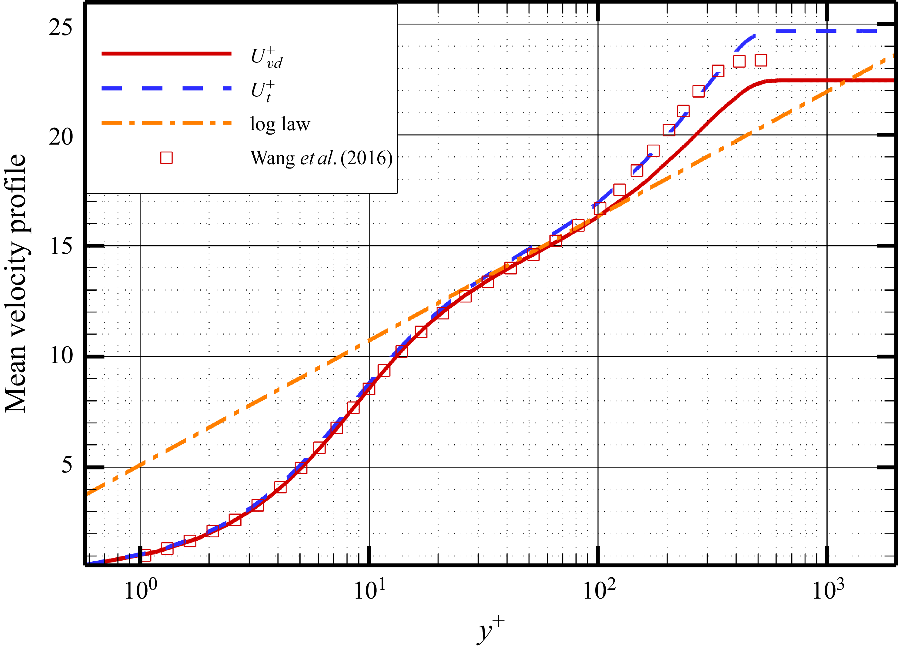
To validate the accuracy of computation, the mean velocity profile after van Driest transformation and Griffin transformation (Griffin, Fu & Moin Reference Griffin, Fu and Moin2021) is depicted in figure 2, where ${U}_{vd}$ is the van Driest transformation ${{U}_{vd}^+}=\int _{0}^{{{u}^{+}}}{(}\bar {\rho }/{{\bar {\rho }}_{w}}{{)}^{1/2}}\,\text{d}{{u}^{+}}$ , and the Griffin transformation is defined as

(2.1) \begin{align} U_{t}^{+}({{y}^{*}})=\int {S_{t}^{+}}\,{\rm d}{{y}^{*}}, \\[-28pt] \nonumber \end{align}

(2.2) \begin{align} {{y}^{*}}=\frac {y}{\nu (y)}\sqrt {\frac {{{\tau }_{w}}}{\rho (y)}}, \\[-28pt] \nonumber \end{align}

(2.3) \begin{align} S_{t}^{+}=\frac {{{\tau }^{+}}S_{\textit{eq}}^{+}}{{{\tau }^{+}}+S_{\textit{eq}}^{+}+S_{TL}^{+}}, \\[-28pt] \nonumber \end{align}

(2.4) \begin{align} S_{TL}^{+}({{y}^{*}})={{\mu }^{+}}\frac {\partial {{U}^{+}}}{\partial {{y}^{+}}}, \\[-28pt] \nonumber \end{align}

(2.5) \begin{align} S_{\textit{eq}}^{+}({{y}^{*}})=\frac {1}{{{\mu }^{+}}}\frac {\partial {{U}^{+}}}{\partial {{y}^{*}}}. \\[-2pt] \nonumber \end{align}

Figure 2.

The mean velocity profile after van Driest transformation and Griffin transformation. The square symbols are the experimental data from Wang, Wang & Zhao (Reference Wang, Wang and Zhao2016), and the dash-dotted line is the log law $U_{vd}^+=\log(y^+)/0.41+5.1$ .

From figure 2, both transformations collapse well with the logarithmic law and the data from Wang et al. (Reference Wang, Wang and Zhao2016). Figure 3 shows the mean skin-friction coefficient curve, which aligns well with the theoretical formula from White (Reference White1974) in the fully developed region.

Figure 3.

The mean skin-friction coefficient. Skin-friction coefficients are normalised by free-stream dynamic pressure, and the dashed line is the theoretical formula from White (Reference White1974).

Figure 4 shows the density-scaled turbulent intensity and Reynolds shear stress, defined as $ (uu )_{\textit{rms}}^+=\sqrt {\overline {\rho }/\overline {\rho }_w}\,\sqrt {\overline {u^{\prime 2}}}/u_\tau$ , $ (vv )_{\textit{rms}}^+=\sqrt {\overline {\rho }/\overline {\rho }_w}\,\sqrt {\overline {v^{\prime 2}}}/u_\tau$ , $ (ww )_{\textit{rms}}^+=\sqrt {\overline {\rho }/\overline {\rho }_w}\,\sqrt {\overline {w^{\prime 2}}}/u_\tau$ , $ (uv )_{\textit{rms}}^+=(\overline {\rho }/\overline {\rho }_w)\,\overline {uv}/u_\tau ^{\prime 2}$ , which exhibit great consistency with the data from Wang et al. (Reference Wang, Wang and Zhao2016). Figure 5 shows the spanwise premultiplied spectra $k_zE^+_{uu}$ . The spectra reach maximum at $\lambda _z^+\approx 100$ and $y^+\approx 10$ , which coincides with the spectra of Kametani (Reference Kametani2017) and Fan & Li (Reference Fan and Li2023).

Figure 4.

The density-scaled turbulent intensity and Reynolds shear stress.

Figure 5.

The spanwise premultiplied spectra $k_zE^+_{uu}$ , where $\lambda _z^+$ and $y^+$ use logarithmic coordinates.

2.2. Clustering method

The clustering method, originally developed by Moisy & Jiménez (Reference Moisy and Jiménez2004) for vortex structure identification in three-dimensional isotropic homogeneous turbulence, has been successfully adapted for RSS analysis. Subsequent applications include the work of Lozano-Durán et al. (Reference Lozano-Durán, Flores and Jiménez2012) in incompressible channel turbulence, and Dong et al. (Reference Diaz-Daniel, Laizet and Vassilicos2017) in homogeneous shear turbulence, demonstrating the method’s versatility across different flow configurations. For compressible turbulent flows, where the Reynolds shear stress is defined as $\tau = -(\rho u)'v'$ , the corresponding RSS are characterised as three-dimensional connected domains satisfying the condition

(2.6) \begin{align} \left | \tau \left ( x,y,z \right ) \right |\gt H\,{{\tau }_{\textit{rms}}}\left ( y \right ), \end{align}

where $H$ is a constant threshold, and ${\tau }_{\textit{rms}}$ is the root mean square of the Reynolds shear stress fluctuations. For flat-plate turbulent boundary layers, $\tau _{\textit{rms}}$ demonstrates wall-normal variation and is characterised as a function of wall distance, denoted as $\tau _{\textit{rms}}(y^+)$ . For different quadrants of Reynolds stress, the structures can be classified into four types based on the signs of $u'$ and $v'$ : Q1 $({{(\rho u)}^{\prime }}\gt 0,\text{ }{v}'\gt 0)$ , Q2 $({{(\rho u)}^{\prime }}\lt 0,\text{ }{v}'\gt 0)$ , Q3 $({{(\rho u)}^{\prime }}\lt 0,\text{ }{v}'\lt 0)$ , and Q4 $({{(\rho u)}^{\prime }}\gt 0,\text{ }{v}'\lt 0)$ . Each type of structure will be identified independently.

Figure 6.

Reynolds stress Q4 structure in the turbulent boundary layer of a supersonic flat plate, coloured by $y^+$ .

The selection of threshold $H$ critically affects the identification of coherent structures. Excessively high thresholds yield undersized structures, while overly low thresholds produce excessively large structures, both scenarios failing to accurately capture the intrinsic properties of coherent motions. To address this problem, Moisy & Jiménez (Reference Moisy and Jiménez2004) adapted percolation theory from disordered systems and random geometry studies (Stauffer & Bunde Reference Stauffer and Bunde1987) to objectively determine the optimal threshold. This part will be discussed in detail in Appendix A. The results indicate that the threshold for both Q2 and Q4 structures can be chosen as $H=1$ .

Applying the determined thresholds, the clustering method effectively isolates RSS within the flow field. Figure 6 illustrates representative Q4 structures in an instantaneous flow, coloured by $y^+$ . These structures exhibit topological characteristics consistent with incompressible channel turbulence observations reported by Lozano-Durán & Jiménez (Reference Lozano-Durán and Jiménez2014), demonstrating the method’s robustness across different flow regimes. 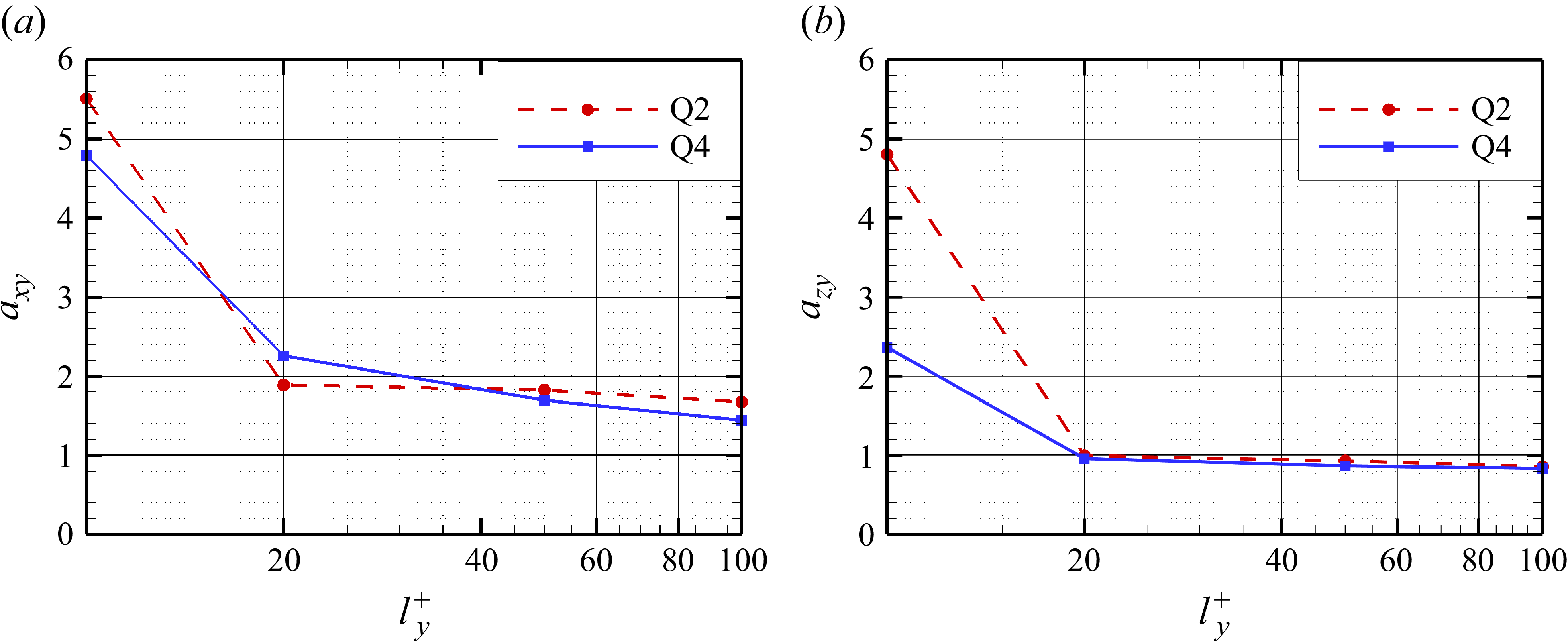The anisotropies $a_{\textit{xy}}=l_x^+/l_y^+$ and $a_{zy}=l_z^+/l_y^+$ of wall-attached Q2 and Q4 with increasing wall-normal scales are shown in figure 7. For small structures near the wall, viscous effects induce pronounced streamwise elongation of Q2 and Q4 structures, forming slender shapes and larger $a_{\textit{xy}}$ , where $a_{\textit{xy}}$ gradually diminishes with increasing scales because of the weakening viscous influence and the stronger main flow. The $a_{\textit{xy}}$ values of the Q2 and Q4 structures are approximately identical, whereas their $a_{zy}$ values exhibit significant differences at small scales, with the spanwise scale of Q4 structures being smaller than that of Q2. However, as the scale increases, the $a_{zy}$ values of both structures converge towards unity. In the compressible channel flow studied by Li et al. (Reference Li, Fu and Xu2025), the RSS follow $l_x^+ \approx 25(l_y^+)^{0.7}$ and $l_z^+ \approx l_y^+$ . The value of $a_{zy}$ in the present work is consistent with theirs; however, the relationship between streamwise and wall-normal scales differs from the nonlinear correlation reported by Li et al. (Reference Li, Fu and Xu2025). This discrepancy may arise because the present study does not employ joint probability density functions to compute $a_{\textit{xy}}$ , relying instead on simple averaging for statistical characterisation. Nevertheless, as this is not the primary focus of our investigation, the averaged $a_{\textit{xy}}$ obtained here is sufficient for subsequent analysis.

Figure 7.

Anisotropy of wall-attached Q2 and Q4 for (a) $a_{\textit{xy}}=l_x^+/l_y^+$ , (b) $a_{zy}=l_z^+/l_y^+$ , where $l_x^+$ , $l_y^+$ and $l_z^+$ are lengths of RSS in the streamwise, wall-normal and spanwise directions, respectively.

Following the identification of RSS in each instantaneous flow field, the overlap ratio between spatially coincident structures across consecutive time steps is computed. For a structure at time $t_1$ with volume $v_1$ , and its overlapping counterpart at $t_2$ with volume $v_2$ , the overlap ratio $R$ is defined as $R = |v_2 - v_1|/v_0$ , where $v_0$ represents the intersecting volume. Notably, a single structure at $t_1$ may overlap with multiple structures at $t_2$ . The minimal overlap ratio $R_{\textit{min}}$ identifies the primary evolutionary path, indicating structural continuity with minimal morphological change. Conversely, when multiple $t_1$ structures overlap with a single $t_2$ structure, this represents structural merging. To efficiently capture these complex evolutionary processes, we implement a directed graph (digraph) representation, where nodes represent individual turbulent structures, directed edges indicate temporal progression, node weights encode physical properties (position, scale, Reynolds stress, etc.), and edge weights store overlap ratio $R$ . This graph-based approach achieves significant storage compression while enabling sophisticated evolutionary analysis. For individual structure evolution studies, we focus exclusively on the primary development path corresponding to $R_{\textit{min}}$ , excluding splitting/merging events. Figure 8 illustrates a representative developmental sequence for a large-scale Q4 structure, revealing predominant streamwise expansion with concurrent growth in both streamwise and spanwise scales throughout its evolution.

Figure 8.

Evolution of a large-scale Q4 structure.

2.3. Conditional skin-friction decomposition

After identification of RSS, a conditionally averaged FIK-like identity will be proposed.

Step 1. Determine the centre point and domain extent for conditional averaging. The conditional averaging procedure employs a computational domain centred on each RSS geometric centre, with dimensions selected as $-150\lt \Delta x^+\lt 150$ , $0\lt y^+\lt 250$ and $-80\lt \Delta z^+\lt 80$ . The wall-normal extent of the conditional averaging domain is selected such that it is greater than the logarithmic region but less than the boundary layer thickness, a height sufficient to resolve structural details. The streamwise and spanwise dimensions, on the other hand, are determined by the scale of the large-scale structures. As shown in figure 7, at $l_y^+ = 100$ , the $a_{\textit{xy}}$ and $a_{zy}$ values for Q2 and Q4 structures are approximately 1.5 and 0.8, respectively. This implies that their streamwise and spanwise scales are approximately 150 and 80 viscous units. To be conservative and retain more flow details, these values are multiplied by 2 to define the streamwise and spanwise lengths for conditional averaging.

Step 2. Classify the structures based on their position and scale. Based on the lowest wall-normal position $y^+_{\textit{min}}$ of the structure, it can generally be categorised as an attached structure ( $y^+_{\textit{min}} \lt 20$ ) or a detached structure ( $y^+_{\textit{min}} \gt 20$ ) (Lozano-Durán & Jiménez Reference Lozano-Durán and Jiménez2014; Dong et al. Reference Diaz-Daniel, Laizet and Vassilicos2017; Jiménez Reference Jiménez2018). Consistent with these prior investigations, our analysis focuses specifically on wall-attached Q2 and Q4 structures (illustrated in figure 7), but with stricter attachment criteria ( $y^+_{\textit{min}}=0$ ), as these account for the predominant share of Reynolds shear stress and play a pivotal role in generating skin-friction drag compared to wall-detached RSS. For attached structures, they are classified into four categories based on their normal scale $l_{y}^+=y^+_{\textit{max}}-y^+_{\textit{min}}$ : $l_{yi}^+ \approx 10, 20, 50, 100$ , categorised using logarithmic intervals ( $l_{y1}^+\lt \sqrt {10\times 20}$ , $\sqrt {10\times 20}\lt l_{y2}^+\lt \sqrt {20\times 50}$ , $\sqrt {20\times 50}\lt l_{y3}^+\lt \sqrt {50\times 100}$ , $l_{y4}^+\gt \sqrt {50\times 100}$ ). For convenience, we will abbreviate as $l_{y}^+ = 10$ and so on in this paper. It should be noted that since the attached structures studied subsequently all have $y^+_{\textit{min}} = 0$ (i.e. their lowest point is immediately adjacent to the wall), $l_y^+$ not only represents the wall-normal scale, but also reflects the distance between the structure’s head and the wall.

Step 3. Perform conditional averaging and skin-friction decomposition for structures of different scales. First, all Q2 structures with $l_y^+ = 10$ are traversed to locate their centre points. Within the statistical window surrounding each centre point, conditional averaging is performed on flow field parameters such as velocity. After obtaining the conditionally averaged flow field parameters, a conditional FIK-like identity is applied to decompose the skin friction. Subsequently, based on the spanwise and wall-normal scales of the structures, the decomposed skin-friction terms are spatially averaged. For example, for a Q2 structure with $l_y^+ = 10$ , we have $a_{\textit{xy}} = 5.5$ and $a_{zy} = 4.8$ , which implies $l_x^+ = 55$ and $l_z^+ = 48$ . The spatial averaging is then performed within a range $\pm \Delta x^+ = 27.5$ and $\pm \Delta z^+ = 24$ centred at $\Delta x^+ = 0$ , $\Delta z^+ = 0$ for each skin-friction term. Finally, the above procedure is repeated for Q2 and Q4 structures of different scales.

The conditionally averaged momentum equations and the FIK-like identity are

(2.7) \begin{align} \frac {\partial \bar {\rho }\tilde {u}}{\partial t}+\frac {\partial \bar {\rho }\tilde {u}{{{\tilde {u}}}_{\kern-2pt j}}}{\partial {{x}_{\kern-2pt j}}}+\frac {\partial \bar {\rho }\,{{\widetilde {{u}^{\prime\prime}{u}^{\prime\prime}}}_{j}}}{\partial {{x}_{\kern-2pt j}}}=-\frac {\partial \bar {p}}{\partial x}+\frac {\partial {{{\bar {\tau }}}_{xj}}}{\partial {{x}_{\kern-2pt j}}}, \\[-28pt] \nonumber \end{align}

(2.8) \begin{align} \begin{aligned} & {{\tau }_{xx}}=2\mu \frac {\partial u}{\partial x}-\frac {2}{3}\mu \left ( \frac {\partial u}{\partial x}+\frac {\partial v}{\partial y}+\frac {\partial w}{\partial z} \right )\!, \\& {{\tau }_{\textit{xy}}}=\mu \left ( \frac {\partial u}{\partial y}+\frac {\partial v}{\partial x} \right )\!, \\& {{\tau }_{xz}}=\mu \left ( \frac {\partial u}{\partial z}+\frac {\partial w}{\partial x} \right )\!, \\ \end{aligned} \\[0pt] \nonumber \end{align}

where $\overline {\phi }$ denotes the conditional Reynolds average, $\widetilde {\phi }$ denotes the conditional Favre average, $\tilde {\phi }=\overline {\rho \phi }/\overline {\rho }$ and ${\phi }''=\phi -\tilde {\phi }$ . Based on the above equation, the FIK-like identity is

(2.9) \begin{align} {{C}_{f}}=C_{\kern-2pt f}^{M}+C_{\kern-2pt f}^{T}+C_{\kern-2pt f}^{P}+C_{\kern-2pt f}^{B}+C_{\kern-2pt f}^{U}, \\[-28pt] \nonumber \end{align}

(2.10) \begin{align} \left \{ \begin{aligned} & C_{\kern-2pt f}^{M}=-\frac {2}{{{y}_{b}}}\int _{0}^{{{y}_{b}}}{({{y}_{b}}-y)}\left (\bar {\rho }\tilde {u} \frac {\partial \tilde {u}}{\partial x}+\bar {\rho }\tilde {v}\frac {\partial \tilde {u}}{\partial y}+\bar {\rho }\tilde {w}\frac {\partial \tilde {u}}{\partial z} \right )\text{d}y, \\ & C_{\kern-2pt f}^{T}=-\frac {2}{{{y}_{b}}}\int _{0}^{{{y}_{b}}}{\left ( {{y}_{b}}-y \right )}\left ( \frac {\partial \bar {\rho }\widetilde {{u}^{\prime\prime}{u}^{\prime\prime}}}{\partial x}+\frac {\partial \bar {\rho }\widetilde {{u}^{\prime\prime}{w}''}}{\partial z} \right )+\bar {\rho }{u}^{\prime\prime}{v}''\,\text{d}y, \\ & C_{\kern-2pt f}^{P}=-\frac {2}{{{y}_{b}}}\int _{0}^{{{y}_{b}}}{\left ( {{y}_{b}}-y \right )}\frac {\partial \bar {p}}{\partial x}\,\text{d}y, \\ & C_{\kern-2pt f}^{B}=\frac {2}{{{y}_{b}}}\int _{0}^{{{y}_{b}}}\left({\left ( {{y}_{b}}-y \right )}\left ( \frac {\partial {{{\bar {\tau }}}_{xx}}}{\partial x}+\frac {\partial {{{\bar {\tau }}}_{xz}}}{\partial z} \right )+{{{\bar {\tau }}}_{\textit{xy}}}\right)\text{d}y, \\ & C_{\kern-2pt f}^{U}=-\frac {2}{{{y}_{b}}}\int _{0}^{{{y}_{b}}}{\left ( {{y}_{b}}-y \right )}\bar {\rho }\frac {\partial \tilde {u}}{\partial t}\,\text{d}y. \\ \end{aligned} \right . \\[0pt] \nonumber \end{align}

For clarity in subsequent expressions, $C_{\kern-2.5pt f}$ hereafter denotes the conditionally averaged skin-friction coefficient, $C_{f2}$ represents the conditionally averaged skin-friction coefficient for Q2 structures, and $C_{f4}$ for Q4 structures. The upper integration limit $y_b$ is typically set to $y_b=1.3\delta _{99}$ in conventional applications (Wenzel et al. Reference Wenzel, Gibis and Kloker2022), where $\delta _{99}$ represents the boundary layer thickness. However, for wall-attached RSS with varying wall-normal scales $l_y^+$ , this study employs $y_b=l_y^+$ to better capture scale-dependent effects.

Figure 9.

Globally averaged FIK-like identity, where $(C_{\kern-2.5pt f})$ is the original skin-friction coefficient: $(C_{\kern-2.5pt f}^{\textit{sum}})=(C_{\kern-2.5pt f}^M)+(C_{\kern-2.5pt f}^T)+(C_{\kern-2.5pt f}^B)+(C_{\kern-2.5pt f}^P)$ , and all terms are normalised by $(C_{\kern-2.5pt f})$ .

In the globally averaged FIK-like identity (Wenzel et al. Reference Wenzel, Gibis and Kloker2022; Xu et al. Reference Xu, Wang and Chen2022), the friction decomposition terms (denoted by $[C_{\kern-2pt f}]$ ) maintain standard interpretations: $[C_{\kern-2pt f}^{M}]$ denotes the mean convection term representing main flow advection, $[C_{\kern-2pt f}^{T}]$ is the turbulent convection term accounting for turbulent fluctuations, $[C_{\kern-2pt f}^{P}]$ is the pressure gradient term, and $[C_{\kern-2pt f}^{B}]$ is the boundary layer term. However, when applying the conditionally averaged FIK-like identity centred on RSS, some terms acquire distinct physical interpretations that differ fundamentally from previous formulations. The term $C_{\kern-2.5pt f}^{\textit{Mx}} = -({2}/{y_b}) \int _0^{y_b} (y_b - y) ( \bar {\rho } \tilde {u} ({\partial \tilde {u}}/{\partial x}) )\, {\rm d}y$ reflects the influence of streamwise momentum transport by RSS during ejection/sweep events on skin friction. Similarly, $C_{\kern-2.5pt f}^{My} = -({2}/{y_b}) \int _0^{y_b} (y_b - y) ( \bar {\rho } \tilde {v} ({\partial \tilde {u}}/{\partial y}) )\, {\rm d}y$ and $C_{\kern-2.5pt f}^{Mz} = -({2}/{y_b}) \int _0^{y_b} (y_b - y) ( \bar {\rho } \tilde {w} ({\partial \tilde {u}}/{\partial z}) )\,{\rm d}y$ represent the wall-normal and spanwise momentum transports, respectively (see § 4 for details). Compared to the globally averaged drag decomposition method, the unsteady term is $C_{\kern-2.5pt f}^{U}\neq 0$ in conditionally averaged drag decomposition because of the evolution of structures (see § 5). Here, $C_{\kern-2.5pt f}^{P}$ represents the streamwise pressure variation caused by structures, $C_{\kern-2.5pt f}^{B}$ represents the viscous effects of boundary layer, and $C_{\kern-2pt f}^{T}$ reflects variations between different structures (see § 6).

To verify the code of the conditionally averaged FIK-like identity, the result of the globally averaged FIK-like identity is shown in figure 9. Similar to the results of Wenzel et al. (Reference Wenzel, Gibis and Kloker2022) and Xu et al. (Reference Xu, Wang and Chen2022), the turbulent convection term $[C_{\kern-2.5pt f}^T]$ dominates the skin-friction generation, followed by the mean convection term $[C_{\kern-2.5pt f}^M]$ and boundary layer term $[C_{\kern-2.5pt f}^B]$ . 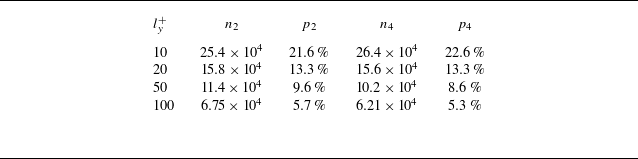The minimal discrepancy ( $\lt 2\,\%$ ) between the reconstructed $[C_{\kern-2.5pt f}^{\textit{sum}}]$ and actual $[C_{\kern-2.5pt f}]$ confirms the accuracy. Table 3 summarises the statistic of conditional averaging. The statistical results of table 3 demonstrate robust dataset characteristics: small-scale Q2/Q4 structures constitute approximately 70 % of the population, and all scale categories contain over $10^4$ samples, ensuring the statistical convergence of conditional averaging. This thorough validation establishes the reliability of our methodology for subsequent scale-dependent analysis of turbulent structures.

Table 3.

Statistics of conditional average: $n_2$ and $p_2$ are the entire number and the percentage of Q2 structures of different scales, and similarly for Q4.