Introduction
The last deglaciation (ca. 20,000–10,000 years ago), also known as the last glacial termination, marked one of the most dynamic climate transitions in Earth’s recent history. This interval was characterized by rapid global warming, the retreat of continental ice sheets, sea-level rise, and abrupt climatic reversals such as Heinrich Stadial 1 (H1), the Bølling-Allerød interstadial (B-A), and the Younger Dryas (YD) cold event (Alley et al., Reference Alley, Clark, Keigwin, Webb, Clark, Webb and Keigwin1999; Clark et al., Reference Clark, Dyke, Shakun, Carlson, Clark, Wohlfarth, Mitrovica, Hostetler and McCabe2009; Denton et al., Reference Denton, Anderson, Toggweiler, Edwards, Schaefer and Putnam2010; Carlson and Clark, Reference Carlson and Clark2012). These rapid changes triggered major reorganizations in terrestrial ecosystems worldwide, influencing vegetation composition, fire regimes, and hydrological systems.
In East Asia, deglacial environmental change was strongly modulated by shifts in the East Asian monsoon system, which in turn is influenced by high-latitude processes such as variations in the Atlantic Meridional Overturning Circulation (AMOC) and by low-latitude ocean–atmosphere interactions, including El Niño–Southern Oscillation (ENSO) variability and latitudinal migration of the Intertropical Convergence Zone (ITCZ) (Cheng et al., Reference Cheng, Sinha, Wang, Cruz and Edwards2012; Mosblech et al., Reference Mosblech, Bush, Gosling, Hodell, Thomas, van Calsteren, Correa-Metrio, Valencia, Curtis and van Woesik2012; Zhang et al., Reference Zhang, Dodson, Chang and Li2021). Palynological records from northern China, the Korean Peninsula, and Japan document northward forest expansion and pronounced ecosystem turnover during this period (Igarashi et al., Reference Igarashi, Yamamoto and Ikehara2011; Shu et al., Reference Shu, Sasaki, Takahara and Hase2013; Wu et al., Reference Wu, Liu, Wang, Chu and Liu2016; Hayashi et al., Reference Hayashi, Takahara, Inouchi, Takemura and Igarashi2017; Yi et al., Reference Yi, Jun, Hong, Choi, Kim, Yoo and Lee2022). Sedimentary charcoal syntheses further indicate intensified wildfire activity, particularly within conifer-dominated forests during cold-dry intervals (Hao et al., Reference Hao, Han, Shu, Zhao, Zhang and An2023; Vachula and Rehn, Reference Vachula and Rehn2023). However, high-resolution inland terrestrial records that simultaneously integrate vegetation, climate, and fire dynamics remain scarce for the Korean Peninsula, where most available archives derive from speleothem or coastal/marine sequences (Chung et al., Reference Chung, Lim and Lee2010; Park et al., Reference Park, Lim, Lim, Yu and Choi2014).
Pollen-based quantitative paleoclimate reconstruction has increasingly been applied beyond the Holocene to Late Pleistocene and deglacial intervals. Reconstructions spanning the last 40 ka in northern Asia (Cao et al., Reference Cao, Tian, Li, Gaillard, Rudaya, Xu and Herzschuh2019), Late Quaternary sequences in Japan (Nakagawa et al., Reference Nakagawa, Tarasov, Nishida, Gotanda and Yasuda2002), Middle Pleistocene deposits in Poland (Pidek and Poska, Reference Pidek and Poska2013), and Late Pleistocene monsoon variability in East Asia (Xiao Zhang et al., Reference Zhang, Zheng, Huang, Cheng, Cheddadi, Zhao and Liang2023) demonstrate the applicability of modern analog and transfer-function approaches under glacial–interglacial boundary conditions. Methodological assessments further confirm that when fossil taxa are well represented within modern calibration datasets, probabilistic pollen–climate transfer methods remain robust for Late Pleistocene applications (Ohlwein and Wahl, Reference Ohlwein and Wahl2012). These advances provide a methodological foundation for extending quantitative pollen-based reconstruction to the last deglaciation.
Here, we present a high-resolution, multiproxy reconstruction from the Gonggeomji paleolake in central inland Korea. Situated within a small mountain-encircled catchment, Gonggeomji functions as an effective sediment trap, preserving detailed records of terrestrial environmental change. By integrating pollen-based quantitative reconstructions of mean annual temperature (PqTann) and precipitation (PqPann), sedimentary charcoal analyses, palynomorph assemblages, and sedimentological proxies, we reconstruct hydroclimate variability between ca. 17,800 and 10,000 cal yr BP. We further evaluate vegetation responses, wildfire disturbance, and ecological resilience under abrupt climate forcing, while assessing the influence of high- and low-latitude drivers on East Asian monsoon dynamics at multi-centennial timescales.
Through this integrated approach, the Gonggeomji record provides a rare inland perspective on land–climate–disturbance feedbacks during the last deglaciation, contributing to a more comprehensive understanding of hydroclimatic variability and ecosystem dynamics in northeast Asia and offering paleoecological analogs for future climate-driven environmental change.
Study area
The Gonggeomji paleolake (36°30′33″–36°30′46″N, 128°09′40″–128°09′55″E) is located in Sangju City in the central inland region of the Korean Peninsula (Fig. 1A). Situated within an alluvial plain at approximately 70 m above sea level (asl), the reservoir occupies a small enclosed basin surrounded by low mountains, including Mt. Sungdeok (214 m asl) to the north, Mt. Obong (235 m asl) to the east, and the Guksa mountain range (337.7 m asl) to the west. These bedrock uplands, formed approximately 600 Ma, consist primarily of granitic gneiss, gneiss, alkali granite, and quartz porphyry (Lee and Kim, Reference Lee and Kim1968). The topography facilitates the convergence of multiple small streams into the basin, while the only outlet lies to the southeast (Fig. 1B). This hydrogeomorphic setting promotes wetland formation around the reservoir and enables Gonggeomji to function as a natural sediment trap.
(A) Location of the 20GG6 core site at the Gonggeomji paleolake in Sangju City, central inland South Korea. The study area lies within the central temperate zone of deciduous broadleaf forest, based on the modern vegetation map of Korea (modified from Yim and Kira, Reference Yim and Kira1975). DBL F., deciduous broadleaved forest. (B) A 3D topographic map of the Gonggeomji paleolake area showing its small catchment basin. (C) Seasonal variations (2002–2019 CE) in temperature and precipitation in the Sangju area, based on data from the Korea Meteorological Administration (https://data.kma.go.kr). (D) Number of fires over the last decade (2013–2022 CE), indicating a concentration of fire occurrences during the cold, dry winter monsoon season (Korea Forest Service, https://www.forest.go.kr).

Figure 1 Long description
The image A showing a map titled Modern Vegetation Map. A small globe inset appears at the upper left. The main map shows an outlined land area with multiple filled regions and several small oval shapes offshore. A legend lists: Conifer slash subalpine zone; DBLF slash northeastern temperate zone; DBLF slash northwestern temperate zone; DBLF slash south temperate zone; DBLF slash eastern temperate zone; Evergreen slash subtropical zone. A label near the lower part reads Study area. The image B showing a 3D terrain map with a compass marked N, E, S, W. The horizontal axis label reads Longitude left bracket degree E right bracket, with tick labels 36.29 and 36.29. The vertical axis label reads Latitude left bracket degree N right bracket, with tick labels 128.16 and 128.16. A label on the map reads Gonggeomji. Another label reads 20GG6. A scale bar at the lower right shows 0, 1.5 and km. The image C showing a combined chart with two vertical axes and a month axis. Text above the plot reads Sangju, 12.7C, 1157 mm and 2002 to 2019. The left vertical axis label reads T left parenthesis C right parenthesis, with tick labels 0, 10, 20, 30. The right vertical axis label reads P left parenthesis mm right parenthesis, with tick labels 0, 50, 100, 200, 300. The horizontal axis label reads Month, with tick labels 1 through 12. A filled shape spans months 1 to 12, rising to a single peak around months 7 to 8 and returning toward the baseline by month 12. A line runs across the months with a low point near month 1, rising toward mid year and then declining toward month 12. The image D showing a bar chart titled Monthly fires for 2013 to 2022 year. The horizontal axis label reads Month, with tick labels 1 through 12. The left vertical axis label reads No. of fire, with tick labels 0, 20, 40, 60, 80, 100, 120, 140. Bars are shown for months 1 through 12, with the tallest bars at months 3 and 4, shorter bars at months 2, 5 and 6, very small bars around months 7 to 9 and moderate bars at months 10 to 12.
Climatically, the region exhibits a continental-type pattern due to its inland basin location. Temperature generally decreases with elevation toward the northwest, whereas the Sangju lowland to the southeast experiences relatively warmer conditions, producing an east–west thermal gradient. The annual mean temperature is approximately 13°C, and mean annual precipitation is 1284.8 mm (Korea Meteorological Administration, https://data.kma.go.kr; Fig. 1C).
The vegetation surrounding Gonggeomji belongs to the central temperate deciduous broadleaf forest zone (Yim and Kira, Reference Yim and Kira1975; Fig. 1A). Dominant woody species include Pinus koraiensis Siebold & Zucc., Quercus variabilis Blume, Q. acutissima Carruth, Q. aliena Blume, Salix chaenomeloides Kimura, and Buxus microphylla var. koreana Nakai ex Rehder. Herbaceous and aquatic plants such as Euphorbia pekinensis Rupr., Alisma orientale (Sam.) Juz., Sagittaria aginashi Makino, Rumex crispus L., Chenopodium ficifolium Smith, C. glaucum L., Phytolacca americana L., Aster pilosus Willd., Taraxacum officinale Weber, Xanthium strumarium L., Panicum dichotomiflorum Michx., Nymphoides peltata (J.G. Gmelin) Kuntze, Ajuga multiflora Bunge, Potamogeton octandrus Poir., and Monochoria korsakowii Regel & Maack are common in wetland habitats (Song and Park, Reference Song and Park2013). This modern vegetation composition provides useful analogs for interpreting Holocene palynological data.
The Gonggeomji embankment, constructed mainly of clay and sandy soils, retains sediments continuously supplied from adjacent hillslopes and tributaries. Previous coring studies confirm that sediment accumulation has occurred since at least the Late Holocene, yielding stratigraphic sequences rich in diatoms and pollen—key proxies for reconstructing past environmental conditions (Yoon et al., Reference Yoon, Ahn, Kim and Hwang2013). Depositional processes in this catchment are regulated by both natural and anthropogenic factors. Hydrological variability, topographic gradients, vegetation cover, stream discharge, and fluid dynamics interact with human influences such as embankment construction and lowland agriculture to shape sedimentation patterns. These integrated processes are archived in well-stratified sediment layers, which serve as valuable paleoenvironmental records (Hwang et al., Reference Hwang, Kim and Yoon2014).
Materials and methods
Fieldwork
Two sediment cores, 20GG6-1 and 20GG6-2 (36°30′31″N, 128°08′42″E; elevation 67.32 m above sea level), each 8 m in length, were collected from the paddy levee with the objective of splicing them to recovering a complete core sequence (Figs. 1B and 2). Coring was conducted using a rotary drilling corer fit with PVC liners (10 cm diameter, 100 cm length). The recovered sediments were transported to the KIGAM Laboratory, where they were unpacked, cleaned, and cut into 1 cm slices.
Radiocarbon ages
To establish a robust chronology, 14 terrestrial plant fragments from cores 20GG6-1 and 20GG6-2 were radiocarbon dated at the Korea Institute of Geoscience and Mineral Resources (Table 1). The use of terrestrial plant macrofossils minimizes potential reservoir effects commonly associated with aquatic materials.
Accelerator mass spectrometry (AMS) radiocarbon dating results for the 20GG6-1 and 20GG6-2 sediment cores from the Gonggeomji paleolake in Sangju City, central inland South Korea.

Table 1 Long description
The table lists accelerator mass spectrometry radiocarbon dating results for two sediment cores, reporting core depth, carbon isotope values, radiocarbon age with uncertainty, calibrated age ranges, sample material, lab codes, and which core each sample came from. All samples are plant fragments and span depths from 605 to 774 centimeters. Calibrated ages range from about 15,050 to 16,140 calendar years before present, corresponding to roughly 13,105 to 14,190 BCE. The youngest calibrated age is at 625 cm in core 20GG6-2, while the oldest is at 774 cm in core 20GG6-1. In core 20GG6-1, deeper samples generally correspond to older calibrated ages, though there are small reversals around 667 to 680 cm where ages are very similar. Carbon isotope values vary widely, from about minus 19.49 to minus 32.11 per mil, with the most negative value at 753 cm. Reported uncertainties are on the order of about 58 to 79 years for radiocarbon ages and about 210 to 250 years for calibrated ages, so close ages may not be meaningfully different.
Although most radiocarbon ages follow a stratigraphically consistent order, several younger age inversions were identified. These anomalously young ages are most plausibly attributed to downward penetration of plant roots into older sediment layers, a well-documented process in wetland and lacustrine environments that can yield ages younger than the true depositional age.
An age–depth model was constructed using OxCal with the IntCal20 calibration dataset (Reimer et al., Reference Reimer, Austin, Bard, Bayliss, Blackwell, Bronk Ramsey and Butzin2020) and implemented in R using the Clam package (Blaauw, Reference Blaauw2010; Fig. 2B). Dates inconsistent with stratigraphic order and falling outside the 95% confidence envelope of the modeled age–depth relationship were excluded from the final model to ensure chronological coherence. The resulting model, based on statistically robust and internally consistent ages, provides the temporal framework for subsequent paleoenvironmental interpretations.
Two cores (20GG6-1 and 20GG6-2) were drilled to create a scientific splice covering the entire Gonggeomji paleolake sequence. (A) Lithology column, calibrated ages, grain-size analysis, and generalized core description. (B) Photograph of the studied core section and age–depth model (Clam software). Dark gray shading shows the most likely calendar ages; gray stippled lines indicate 95% confidence intervals; the black curve represents the single “best” model based on the median age for each depth.

Figure 2 Long description
The image consists of two panels. The first panel shows a stratigraphic log with a grain-size curve for sediment cores. The x-axis is labeled ′Grain Size (μm)′ ranging from 0 to 500. The y-axis is labeled ′Depth (m)′ ranging from 0 to 8. Key layers are annotated, including gravelly gray to greenish brown silty to sandy clay, coarse sand and organic fragments. Sampling points are marked. The second panel displays an age-depth model. The x-axis is labeled ′Age (cal yr BP)′ ranging from 12000 to 14000. The y-axis is labeled ′Depth (m)′ ranging from 5 to 8. A black curve represents the median age model, with dark gray shading indicating the most likely calendar ages and gray stippled lines showing 95 percent confidence intervals. Notable dated levels are highlighted, showing a monotonic increase of age with depth. Uncertainty bands widen at certain intervals.
Grain size
Sixty-eight samples were pretreated with 5% H₂O₂ to remove organic matter and 5% HCl to remove carbonates. The remaining residues were wet-sieved through metal sieves and classified into the following fractions: 16 mm, 8 mm, 4 mm, 2 mm, 1 mm, and <1 mm. Particles smaller than 1 mm were analyzed using a Mastersizer 2000 laser analyzer (Malvern Instruments, Malvern, UK) (Fig. 2A).
Palynology and sedimentary charcoal
Seventy-four samples from cores 20GG6-1 and 20GG6-2 were collected for pollen analysis at 2.5 and 5 cm intervals from 5.0 to 8.6 m depth (Fig. 2). Pollen extraction followed the standard method of Moore et al. (Reference Moore, Webb and Collison1991). Two tablets containing exotic Lycopodium spores (27,637 ± 563 spores/tablet) were added to each dry sample (2–4 g) to calculate pollen concentration (Stockmarr, Reference Stockmarr1971). A minimum of 250 terrestrial pollen grains were counted, and pollen percentages were calculated relative to the total terrestrial pollen sum.
Palynomorph identification was conducted using a Leica DM6 B optical microscope at 200× and 400× magnifications, based on reference atlases of pollen from northern East Asia (Chang, Reference Chang1986; Chang and Rim, Reference Chang and Rim1979) and freshwater algae from lacustrine sediments worldwide (van Geel, Reference van Geel, Smol, Birks and Last2001). Diagnostic morphological features of the coniferous bisaccate pollen identified in this study are provided in the Supplementary Information (Supplementary Fig. S1). A palynomorph diagram with local pollen assemblage zones (LPAZs) was constructed using TILIA v. 2.0.41 (Grimm, Reference Grimm2011).
Charcoal particles (<200 µm) on the pollen slides were counted concurrently. Microcharcoal (20–50 μm) was interpreted as representing regional fires, whereas macrocharcoal (>150 μm) was interpreted as representing local fires, based on major axis dimensions. Sedimentary charcoal concentrations were calculated following Vachula (Reference Vachula2019), with more than 500 particles counted per sample. The macrocharcoal to microcharcoal (Ma/Mi) ratio was also calculated to estimate the relative contribution of local versus regional biomass burning (Whitlock and Larsen, Reference Whitlock, Larsen, Smol, Birks and Last2001; Enache and Cumming, Reference Enache and Cumming2006).
Ordination analysis of palynomorph assemblage
Ordination analyses were performed using the vegan package in R (Oksanen et al., Reference Oksanen, Simpson, Blanchet, Kindt, Legendre, Minchin and O’Hara2022), and biplots were generated with the ggplot2 package (Wickham, Reference Wickham2016). Principal component analysis (PCA) included only taxa contributing more than 1.0% in at least three samples to ensure robustness. Pollen-based reconstructions of mean annual temperature (PqTann) and annual precipitation (PqPann) were performed independently using the Climate REconstruction SofTware (CREST) platform (Chevalier et al., Reference Chevalier, Cheddadi and Chase2014) with a GBIF-formatted reference dataset for the Korean Peninsula (Chevalier, Reference Chevalier2019). The dataset included 5123 plant distribution records across 450 grid cells (0.25° resolution) for the study region. A Butterworth low-pass filter was applied to the reconstructed climate curves to highlight multi-centennial- to millennial-scale hydroclimatic variability.
Wood anatomy
Wood identification was conducted on three wood fragment samples from core 20GG6-1 by the Tree-Ring Research Center (TRRC) of Chungbuk National University. Preparation for microscopic anatomical analysis involved:
1. Cutting cross, tangential, and radial sections to an appropriate thickness for optical microscopy using a razor blade.
2. Mounting the sections on glass slides and covering with coverslips using 50% glycerin jelly.
3. Observing and photographing the sections with a Nikon ECLIPSE 80i optical microscope.
Identification followed Identification of Wood Anatomy (Park et al., Reference Park, Lee and Lee1987), Properties and Uses of Wood Species in Korea I (Lee, Reference Lee1997), and Wood Properties of the Useful Tree Species Grown in Korea (Jeong and Park, Reference Jeong and Park2008), with final confirmation being made through comparison with reference specimens at the NITE Research Center.
Results
Lithology and Chronology
The lower section (8.0–5.0 m) of the 20GG6 core, from which pollen, sedimentary charcoal, and grain-size analyses were conducted, exhibits a prominent fining-upward sequence. The lower to middle portions consists mainly of fine to medium sand interbedded with thin layers of greenish silty clay. The upper part transitioned into greenish-gray to greenish-brown silty to sandy clay, showing a gradual upward decrease in grain size (Fig. 2A).
The age model for the studied section of the 20GG6 core was constructed using the Clam package in R (Blaauw, Reference Blaauw2010), based on 14 calibrated radiocarbon ages obtained from plant fragments and applying linear interpolation and extrapolation to establish the age–depth relationship (Fig. 2B). The dated interval spans approximately 2 m of sediment thickness, providing a relatively dense chronological framework for the analyzed section. Although no radiocarbon dates were obtained from the uppermost part corresponding to the Early Holocene, ages for this interval were estimated by extrapolation of the established age–depth model.
The resulting model indicates that the spliced sedimentary sequence from cores 20GG6-1 and 20GG6-2 covers approximately 17,800 to 10,000 cal yr BP, encompassing the entire last deglaciation. The extrapolated Early Holocene ages are internally consistent with the overall sedimentation trend and are further supported by stratigraphic shifts in pollen assemblages, including an increase in warm-temperate deciduous taxa and moisture indicators, together with an apparent decline in boreal conifers, consistent with the expected onset of Early Holocene conditions. Collectively, these results provide a coherent and robust temporal framework for interpreting hydroclimatic and vegetation changes recorded in the core.
Local palynomorph assemblage zone
A total of four LPAZs (LPAZ I–IV), including three subzones within LPAZ III, were established from the 20GG6 core based on statistically significant changes in arboreal pollen taxa using CONISS cluster analysis implemented in TILIA v. 2.0.41 (Grimm, Reference Grimm2011; Fig. 3). The studied section (8.0–5.0 m) yielded abundant and well-preserved pollen and non-pollen palynomorphs (NPPs), except for the basal 860–795 cm interval, where coarse gravel-rich sand prevented pollen deposition and preservation; this interval was therefore classified as barren.
Palynomorph diagram showing selected taxa and sedimentary charcoal from the 20GG6 sediment core. Four local pollen assemblage zones (LPAZs) with three subzones were defined based on critical taxa and statistical analysis using CONISS. Pollen groups are classified according to ecological habitat. Gray shading of individual taxa is presented with 3× exaggeration. T-C-C denotes Taxaceae–Cephalotaxaceae–Cupressaceae.

Figure 3 Long description
The diagram is a stratigraphic pollen percentage multi-panel plot from the 20GG6 sediment core. Each panel represents a separate taxon or pollen group, with the x-axis of each panel showing relative abundance in percent and the y-axis shared across all panels showing depth in centimeters, running from approximately 800 centimeters at the base to 500 centimeters at the top. A dendrogram produced by CONISS cluster analysis appears on the right side of the diagram and defines the boundaries of four local pollen assemblage zones labeled LPAZ I, LPAZ II, LPAZ III and LPAZ IV. LPAZ III contains three subzones. The basal interval from approximately 860 to 795 centimeters is marked as barren, indicating no pollen recovery. LPAZ I occupies the lowermost productive interval above 795 centimeters. LPAZ II, LPAZ III with its three subzones and LPAZ IV succeed it upward toward 500 centimeters. Pollen groups are arranged by ecological habitat across the panels, with arboreal taxa displayed in the left portion of the diagram and non-arboreal taxa in the central portion. A dedicated panel for sedimentary charcoal appears toward the right side of the diagram. Individual taxon curves are shown with gray shading and each curve is presented at three times exaggeration, meaning the plotted values are scaled by a factor of three relative to actual abundance to improve visibility of low-percentage taxa. The taxon T-C-C, denoting Taxaceae-Cephalotaxaceae-Cupressaceae, is one of the labeled arboreal groups. Arboreal pollen panels show varying abundance peaks across the defined zones, with shifts in dominant taxa visible at the zone boundaries identified by the CONISS dendrogram. The charcoal panel shows fluctuating values across the depth range, with notable variation within the LPAZ III interval. The CONISS dendrogram on the far right groups depth levels into the four main zones, with branch lengths indicating the degree of compositional change at each boundary.
LPAZ I (ca. 16,500–15,280 cal yr BP; 795–760 cm) was characterized by low pollen concentrations (mean: 1022 grains/g; range: 0–2874) and dominance of boreal conifers, including Picea, Abies, and Pinus subgen. Haploxylon, with contributions from Larix and the cold-tolerant deciduous broadleaved tree Betula, together with temperate deciduous broadleaved Quercus. Artemisia, a xerophytic herb, occurred exclusively in this zone. The low pollen density and coarse-grained matrix suggested limited local vegetation cover and a poorly developed depositional setting.
LPAZ II (ca. 15,280–14,800 cal yr BP; 755–740 cm) maintained similarly low pollen concentrations (mean: 3582 grains/g; range: 442–6412) and was dominated by boreal conifers (Picea, Pinus subgen. Haploxylon), with associated taxa including Larix, T-C-C (Taxaceae–Cephalotaxaceae–Cupressaceae), Betula, and Quercus. Artemisia disappeared, while aquatic indicators such as the freshwater alga Spirogyra and the fungal NPP Glomus became prominent. Numerous stomatal fragments, likely from conifer tissues, further supported the local dominance of evergreen needleleaf vegetation.
LPAZ III (ca. 14,800–11,600 cal yr BP; 737–575 cm) represents the interval of highest pollen concentration in the profile (mean: 19,675 grains/g; range: 2653–53,063). It records an expansion of boreal conifers (Picea, Pinus subgen. Haploxylon, Abies, Larix, T-C-C) and an increase in temperate deciduous broadleaved taxa (Quercus, Myrica, Acer, Rhus, Carpinus, Corylus, Rhododendron, and Ulmus/Zelkova). Herbaceous pollen, including Cyperaceae, Poaceae, Geranium, and persistent Artemisia, was also present. The consistent occurrence of Spirogyra and abundant monolete spores persists throughout the zone.
This zone was divided into three subzones: III-a was marked by rising Picea and Pinus subgen. Haploxylon; III-b shows a sharp decline in Larix, Betula, and Quercus with a drop in pollen concentration; and III-c indicates renewed increases in concentration with diversification of deciduous broadleaved taxa and herbaceous components.
LPAZ IV (ca. 11,600–10,040 cal yr BP; 570–500 cm) shows a gradual decline in pollen concentration from base to top (mean: 7944 grains/g; range: 2432–14,150). Boreal conifers such as Picea and Pinus subgen. Haploxylon sharply decrease and disappear upward, while T-C-C and temperate broadleaved taxa (Quercus, Carpinus, and Ulmus/Zelkova) remained moderately abundant. Herbaceous taxa, including Lychnis, Cirsium, Geranium, and Artemisia, occur at low frequencies. Monolete moss spores and trilete fern spores (e.g., Osmunda) are notably dominant.
Numerical analysis (ordination analysis)
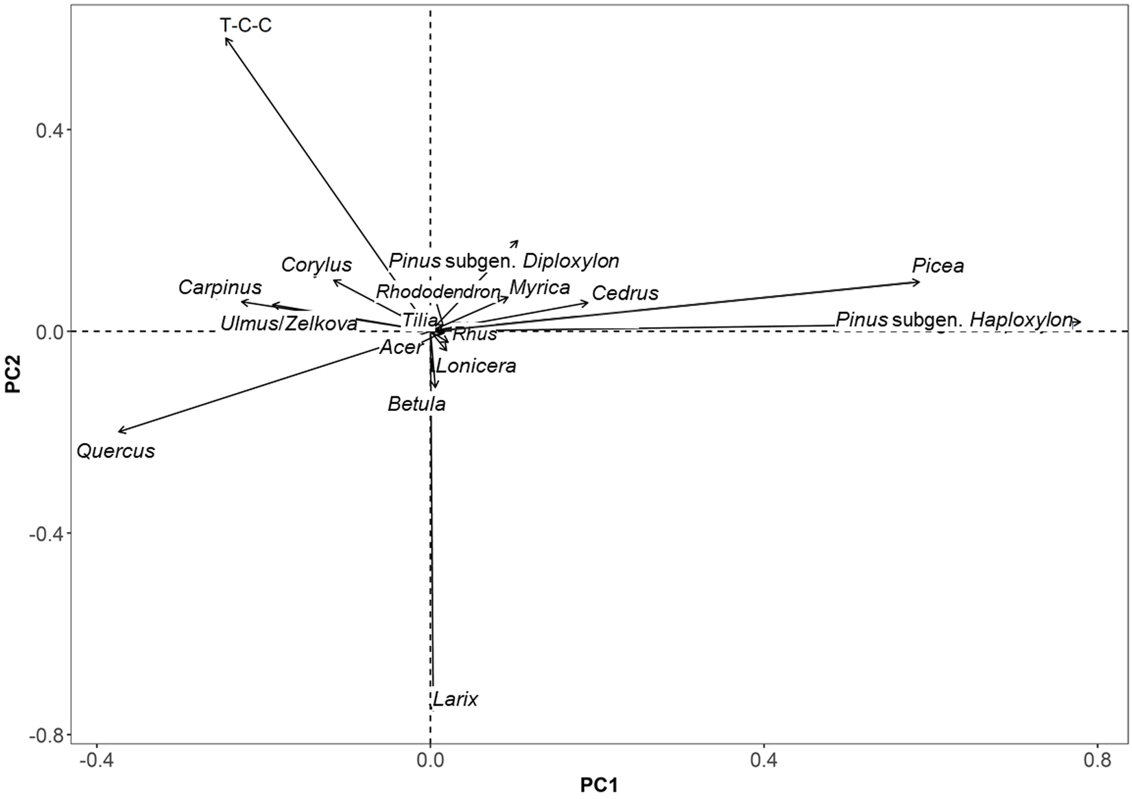
To identify the major ecological gradients and climatic patterns in the arboreal pollen data, PCA was performed on the 20GG6-1 core dataset. Before ordination, pollen percentages were Hellinger-transformed to accommodate the compositional structure of the dataset and minimize the influence of rare taxa, thereby improving ecological interpretability.
The PCA was conducted on taxa with relative abundances exceeding 1.0% in at least three samples to ensure ecological relevance and statistical robustness. The resulting ordination (Fig. 4) separated samples along two primary gradients. PC1 accounted for the largest proportion of variance and primarily reflected a temperature gradient, with thermophilous taxa (e.g., Quercus, Carpinus) positively associated and cold-adapted conifers (e.g., Abies, Picea) negatively associated. PC2 was interpreted as a humidity gradient, indicated by the distribution of mesic versus xeric taxa.
Ordination diagram generated by principal component analysis (PCA) of tree and shrub pollen (>1.0% abundance in at least three samples) from the 20GG6 core, showing relationships between taxa (arrows) and climate variables (temperature and precipitation) over time.

Statistically significant correlations supported this interpretation: PC1 was strongly positively correlated with mean annual temperature (PqTann, R 2 = 0.6241), and PC2 was moderately correlated with annual precipitation (PqPann, R 2 = 0.2357) during 17,000–10,000 cal yr BP. These results support the use of PCA-derived axes as proxies for paleotemperature and paleo-humidity.
Temporal trends in PC1 and PC2 corresponded with known climatic phases of the last deglaciation, including H1, the B-A, the YD, and the Early Holocene. PC1 minima align with the H1 and YD cooling events, while PC2 variability captures hydrological fluctuations potentially related to monsoon strength and fire activity. These axes were subsequently used with other proxy records (e.g., charcoal concentration and pollen concentration) to interpret hydroclimate–vegetation–fire dynamics in central inland Korea during the last deglaciation.
Wood identification of plant fragments
Wood cells vary in type, shape, arrangement, and intercellular spaces depending on the tree species, enabling species identification through macroscopic or microscopic observation. Microscopic features therefore allow anatomical differentiation. All three plant fragments sampled from depths of 617.5, 642.5, and 682.5 cm in core 20GG6-1 were identified as Picea spp. (Fig. 5).
Wood fragments analyzed for anatomical identification from a sample taken at 617.5 cm depth in core 20GG6-1. The specimen was identified as Picea spp.

Figure 5 Long description
A composite scientific figure with a core photograph, a sample label photo and four microscope views of a wood fragment. A vertical core strip is shown with the text 20GG6-1 core. A marked area is indicated on the core. A separate photo shows a label with the text 20GG6-1 and 617.5 cm. Four microscope images are shown with titles and arrow labels. Transverse section. Labels read Vertical intercellular canal and Tree-ring border. A scale bar reads 100 micrometer. Tangential section. Labels read Uniseriate ray and Fusiform ray. A scale bar reads 100 micrometer. Radial section I. Labels read Ray parenchyma cell and Piceoid cross-field pitting. A scale bar reads 10 micrometer. Radial section II. Labels read Radial tracheid and Piceoid pit membrane. A scale bar reads 10 micrometer. Arrows connect the marked core area to the sample label photo and to the microscope images.
The wood anatomical features of Picea spp. (Pinaceae) were as follows:
• Transverse section: Coniferous softwood; small vertical resin canals present; growth rings distinct; gradual transition between earlywood and latewood.
• Tangential section: Radial tissues with uniseriate rays and heterocellular rays containing horizontal resin canals.
• Radial section: Radial tissues comprising radial tracheids and ray parenchyma cells; bordered pits between ray parenchyma cells and axial parenchyma cells of the Piceoid type, with terminal pits present in ray parenchyma cells; bordered pits in radial tracheids relatively angular and closely spaced (Piceoid type); bordered pits in axial tracheids uniseriate.
Based on these features, coniferous softwood, small vertical resin canals, uniseriate rays, horizontal resin canals, Piceoid bordered pits, terminal pits in ray parenchyma cells, and Piceoid pit borders, the specimens were classified as Picea within the family Pinaceae.
Discussion
Local vegetation changes during the last deglaciation
The last deglaciation (∼17,000–10,000 cal yr BP) in East Asia was characterized by abrupt climatic transitions—H1, the B-A, and the YD—that triggered rapid reorganizations in regional vegetation communities. Pollen- and phytolith-based syntheses by Gao et al. (Reference Gao, Niu, Song, Wang, Meng, Yang and Liu2023) indicate a pronounced increase in the rate of vegetation change (ROC) during this interval, driven by shifts in moisture availability, fire frequency, and temperature. ROC values peaked during the deglaciation and declined in the Early Holocene, reflecting heightened ecological instability under climatic stress. Periodicities in ROC (∼1500 and ∼350 years in forests; ∼500 and ∼270 years in grasslands) suggest that solar forcing also contributed to ecosystem turnover.
Complementary palynological evidence from Xu et al. (Reference Xu, Chu, Shen, Sun, Wu, Li, Dong, Cui, Wu and Lu2023a, Reference Xu, Lu, Chu, Shen, Sun, Wu and Li2023b) shows that East Asian vegetation responded sensitively to millennial-scale anomalies, with even short-lived events such as the YD causing notable shifts in arboreal and herbaceous taxa. These observations are consistent with North Atlantic records (Williams et al., Reference Williams, Post, Cwynar, Lotter and Levesque2002; Yu, Reference Yu2003), where forest compositional changes occurred within decades to centuries. High-resolution records from Huadian Cave in northeast China (Niu et al., Reference Niu, Marquer, Sack, Quan and Wang2025) further indicate that, despite a weakened East Asian summer monsoon (EASM), conditions between ∼17,000 and 10,000 cal yr BP remained relatively warm and humid, allowing mesic vegetation to expand. Temperate deciduous trees such as Quercus and Corylus increased gradually, while steppe taxa (Artemisia, Poaceae) persisted in open landscapes. Cold-adapted conifers (Pinus, Abies) remained scarce, suggesting a limited role for boreal elements.
During the H1 period (LPAZ I–II; ∼16,500–14,800 cal yr BP), vegetation in the Gonggeomji paleolake region was dominated by boreal coniferous forests, as indicated by consistently high values of the boreal conifer (BC) pollen index (Fig. 6A) aggregating Picea, Abies, Larix, and Pinus subgen. Haploxylon. The warm-temperate deciduous broadleaved (WTDB) pollen index (Fig. 6B) remained low, indicating that thermophilous taxa such as Quercus, Carpinus, and Ulmus/Zelkova were restricted to microhabitats with localized warmth or shelter. PC1 and PC2 values were negative throughout this period (Fig. 6F and G), reflecting low temperature and reduced humidity. These conditions are consistent with the globally cold, dry climate of H1. The high frequency of Glomus spores (Fig. 6E), associated with soil disturbance, and the near absence of monolete spores (Fig. 6D), linked to moist ground cover, suggest sparsely vegetated lowlands and degraded slopes. Overall, this period was marked by boreal conifer dominance, minimal thermophilous forest expansion, and open, erosion-prone landscapes.
Changes in vegetation communities (A–C), rainfall-driven forest and lowland soil erosion intensity (D and E), and principal component analysis (PCA) axes 1 and 2 (representing temperature and humidity, respectively) from the 20GG6 cores throughout the local pollen assemblage zone (LPAZ) during the last deglaciation. BC and WTDB denote boreal conifers and warm-temperate deciduous broadleaved species, respectively.

Figure 6 Long description
Holocene (11.6 ka) YD (11.6-13.2 ka) B-A (13.2-14.8 ka) H1 (14.8-16.5 ka) Seven stacked line graphs share the x-axis label Age (cal yr BP), with tick labels 11000, 12000, 13000, 14000, 15000, 16000. Vertical divider lines mark the boundaries between the four labeled intervals. Each graph shows two overlaid lines: a jagged line and a thicker smooth curve. Each graph also includes an R superscript 2 value printed inside the plotting area. A. BC (percent). Y-axis tick labels are minus 0.1, 0.4, 0.9. R superscript 2 equals 0.6442. The smooth curve rises from near the lower tick range at about 11000 toward higher values by about 14000 to 15000, then bends downward toward 16000. The jagged line fluctuates around the smooth curve, with larger short spikes near the older end. B. WTDB (percent). Y-axis tick labels are minus 0.1, 0.1, 0.2. R superscript 2 equals 0.1189. The smooth curve stays near the middle of the axis range for much of the record, then turns upward near the oldest ages close to 16000. The jagged line shows frequent narrow spikes, including several higher spikes near the oldest ages. C. Quercus (percent). Y-axis tick labels are 0.0, 0.5, 1.0. R superscript 2 equals 0.2385. The smooth curve is low near 11000, increases gradually toward about 14000 to 15000, then rises more strongly toward 16000. The jagged line varies around the smooth curve with small peaks and dips. D. Monolete (percent). Y-axis tick labels are 0.0, 0.5, 1.0. R superscript 2 equals 0.8893. The smooth curve declines from higher values near 11000 toward lower values by about 14000 to 15000, then remains low toward 16000. The jagged line follows the same overall decline with smaller fluctuations. E. Glomus (count). Y-axis tick labels are 0, 10, 20. R superscript 2 equals 0.1386. The smooth curve stays near the lower part of the scale for most ages, with a slight rise toward older ages. The jagged line shows multiple sharp spikes, including several tall spikes near the oldest ages close to 16000. F. PC1 (temp). Y-axis tick labels are minus 0.8, minus 0.4, 0.0, 0.4, 0.8. R superscript 2 equals 0.6241. The smooth curve increases from lower values near 11000 to a broad high point around about 14000 to 15000, then decreases toward 16000. The jagged line fluctuates around the smooth curve. G. PC2 (humidity). Y-axis tick labels are minus 0.8, minus 0.3, 0.2, 0.7. R superscript 2 equals 0.2357. The smooth curve stays near the middle of the scale from about 11000 through about 14000, then trends downward toward 16000. The jagged line shows short-term variability around the smooth curve. Below the stacked graphs is a dendrogram-like diagram labeled CONISS at the left. At the right of this lower diagram, a vertical scale is labeled Total sum of squares, with tick labels 0 and 20. Along the bottom, zone labels are IV, III-c, III-b, III-a, II, I and Barren.
The subsequent B-A interstadial (LPAZ III-a to III-b; ∼14,800–13,200 cal yr BP) records abrupt climatic amelioration. WTDB pollen values (Fig. 6B) increased sharply, indicating an expansion of Quercus, Carpinus, and Ulmus/Zelkova. This was accompanied by rising PC1 (temperature) and moderately increasing PC2 (humidity) values (Fig. 6F and G). Boreal conifer representation (Fig. 6A) declined, signaling replacement by mixed coniferous–deciduous forests. Monolete spores (Fig. 6D) increased, reflecting improved ground moisture, while Glomus spores (Fig. 6E) decreased, suggesting reduced soil disturbance under denser canopy cover. These changes reflect rapid reorganization of vegetation and hydrological regimes in response to warming.
The YD (LPAZ III-c; ∼13,200–11,600 cal yr BP) brought a return to cooler conditions. BC values (Fig. 6A) increased, WTDB values (Fig. 6B) declined, and PC1 decreased (Fig. 6F). However, PC2 did not decline significantly and even increased slightly (Fig. 6G), implying that moisture availability was maintained despite cooling. Monolete spores persisted (Fig. 6D), and Glomus remained at moderate levels (Fig. 6E), suggesting continued ground moisture and modest soil disturbance. These conditions supported cold-adapted but resilient vegetation, with a mosaic of open and closed forest patches likely maintained by intensified winter monsoon activity and localized fire disturbance (see “Pollen-based Quantitative Hydroclimate Reconstruction”).
From ∼11,600 cal yr BP onward (LPAZ IV), the Gonggeomji record indicates stable, warm, and humid Early Holocene conditions. WTDB taxa increased, boreal conifers declined, and both PC1 and PC2 trend positively (Fig. 6A, B, and F, G), reflecting enhanced temperature and moisture. Low Glomus values suggest reduced soil erosion and improved slope stability, consistent with the establishment of closed-canopy warm-temperate deciduous forests. Monolete spores (moss) reach maximum abundance during this interval (Fig. 6D). They are interpreted not as direct temperature proxies but as indicators of sustained humid air conditions and high soil moisture. Experimental studies show that bryophyte spore release is regulated by atmospheric humidity thresholds (Johansson et al., Reference Johansson, Lönnell, Rannik, Sundberg and Hylander2016), and previous research demonstrates preferential transport and enrichment of fern and moss spores under humid, water-influenced conditions (Li et al., Reference Li, Zhang, Li, Zhang, Li, Liu, Fan and Li2008; Yang et al., Reference Yang, Li, Liu, Li, Wen, Ye, Yi and Chen2016; Song et al., Reference Song, Li, Lu, Mao, Saito, Yi and Lim2017). In the uppermost section, monolete spore dominance co-occurs with aquatic and wetland taxa (e.g., Typha–Sparganium, Nelumbo, Nuphar, Cyperaceae, Poaceae) and freshwater algae (Spirogyra, Pseudoschizaea), supporting the interpretation of sustained hydroclimatic humidity, high soil moisture, and a persistently wet depositional environment during the Early Holocene.
In summary, the Gonggeomji record demonstrates high sensitivity of vegetation to abrupt climatic shifts during the last deglaciation. H1 was marked by cold, dry conditions favoring boreal conifers; the B-A by rapid expansion of warm-temperate deciduous forests; and the YD by a brief cooling phase with moisture maintained. The Early Holocene brought climatic stability and mature forest development. These patterns highlight strong climate–vegetation linkages and underscore Gonggeomji’s value as a midlatitude northeast Asian hydroclimate–ecosystem archive.
Sedimentary charcoal-based wildfire events
Sedimentary charcoal serves as a valuable proxy for reconstructing past wildfire activity and its relationship to climatic shifts and vegetation dynamics. In this study, both macrocharcoal (>150 μm) and microcharcoal (<25–50 μm) were analyzed from the 20GG6 core of the Gonggeomji paleolake to infer local- and regional-scale wildfire episodes during the last deglaciation. The Ma/Mi ratio was also used to infer the relative intensity and proximity of fire events.
Four major peaks in macrocharcoal concentrations—at ca. 15.2, ca. 14.8, ca. 12.6, and ca. 10.5 ka (Fig. 6B)—corresponded to the late H1, the B-A, the terminal YD, and the Early Holocene, respectively. These intervals coincide with elevated Ma/Mi ratios (Fig. 6D), suggesting intensified fire episodes within or near the catchment. Concurrent increases in microcharcoal (Fig. 6C) indicate widespread regional fire activity. These patterns were especially pronounced during the YD, when both macro- and microcharcoal signals align with decreased monolete spore abundance (Fig. 6E), indicating reduced ground vegetation cover and greater surface exposure.
These wildfire events appear closely linked to climatic controls, particularly the East Asian winter monsoon (EAWM). During H1 and the YD, intensification of the Siberian High generated cold, dry northwesterly airflow across the Korean Peninsula, leading to arid conditions during the winter–spring fire season. Under such regimes, resin-rich boreal conifers (Pinus, Abies, Picea) would have been highly flammable. Strong winds likely facilitated ignition through branch friction and enhanced fire spread. Similar processes are observed in modern wildfires in the eastern mountainous region of Korea (Gangwon Province), where natural fuel biomass and meteorological conditions resemble those inferred for the Late Pleistocene (Korea Forest Service, 2023).
Wildfires also triggered landscape-scale feedbacks. As shown in Figure 7, periods of high macrocharcoal abundance coincide with reduced pollen concentrations, particularly of monolete spores and warm-temperate taxa, suggesting that fire-induced vegetation loss reduced pollen input to the basin. Loss of plant cover increased slope exposure, amplifying rainfall-driven soil erosion. Even under modest precipitation, sediment transport was intensified due to reduced vegetation-mediated soil protection. This is reflected in coeval peaks in sand content (Fig. 7A) and increased Glomus spore abundance (Fig. 7G), a fungal taxon associated with disturbed or eroded soils.
Grain-size analysis in relation to rainfall intensity (A), sedimentary macrocharcoal concentrations indicating local wildfires (B), microcharcoal concentrations indicating regional wildfires (C), macrocharcoal/microcharcoal (Ma/Mi) ratio (D), and rainfall-driven forest and lowland soil erosion intensity (E and F) from the 20GG6 cores during the last deglaciation in central inland South Korea.

Figure 7 Long description
The image shows six stacked line graphs representing paleoenvironmental data across different time intervals: Holocene, Younger Dryas, Bølling-Allerød and Heinrich 1. The x-axis is labeled ′Age (cal years BP)′ ranging from 10000 to 16000. The y-axes are labeled as follows: A) Sand content in percent, ranging from 0 to 100; B) Macrocharcoal count, ranging from 0 to 30; C) Microcharcoal count, ranging from 0 to 4; D) Ma slash Mi ratio, ranging from 0 to 4; E) Monolete spores in percent, ranging from 0 to 1; F) Glomus count, ranging from 0 to 20. Each graph includes raw data and a smoothed trend line with R squared values indicating fit quality. Vertical lines mark transitions between periods. Key observations include peaks in sand content around 12000 years BP, macrocharcoal peaks around 13000 years BP and notable increases in Glomus counts around 14000 years BP. The graphs illustrate relationships between variables, such as the correlation between charcoal counts and sand content, indicating environmental changes during the last deglaciation in central inland South Korea.
These interactions are conceptually illustrated in Figure 7. Intensification of the EAWM likely triggered wildfire ignition and rapid spread, leading to canopy destruction and significant vegetation loss. Reduced surface stability enhanced rainfall-induced soil erosion, facilitating the transport of charcoal particles and coarse-grained sediments into the basin. The Gonggeomji record thus captures a tightly coupled disturbance–response–feedback system characteristic of temperate mountain catchments under cold, arid climatic conditions.
The Gonggeomji fire record aligns with other regional studies showing increased fire activity during the last deglaciation in northeast Asia (Inoue et al., Reference Inoue, Okunaka and Kawano2016; Hao et al., Reference Hao, Han, Shu, Zhao, Zhang and An2023). On a broader scale, charcoal synthesis studies across the Northern Hemisphere also report heightened fire frequency during glacial-to-interglacial transitions, often driven by shifts in biomass availability, monsoon dynamics, and temperature seasonality (Power et al., Reference Power, Marlon, Ortiz, Bartlein, Harrison, Mayle and Ballouche2008; Vachula and Rehn, Reference Vachula and Rehn2023; Vachula et al., Reference Vachula, Cullen, Galinger, Welch, Battaglia, Smith and Waters2024).
Pollen-based quantitative hydroclimate reconstruction
Pollen-based quantitative reconstructions of mean annual temperature (PqTann) and mean annual precipitation (PqPann) from the Gonggeomji paleolake provide a high-resolution hydroclimatic record from ca. 16,500 to 10,000 cal yr BP (Fig. 8A–D). These reconstructions were generated using the CREST method, which integrates subfossil arboreal pollen data with a regionally calibrated plant–climate database. The results reveal distinct multi-millennial trends and abrupt shifts corresponding to major climatic events, including H1, B-A, and YD.
Comparison of hydroclimatic changes with potential forcing mechanisms during the last deglaciation. (A–D) Pollen-based quantitative hydroclimate reconstruction at 50 year resolution using the Butterworth filter method from core 20GG6-1 (this study). (E) Two records of East Asian hydroclimate from key El Niño–Southern Oscillation (ENSO)-sensitive regions: Rh/Sr ratios in lake core LC1 from Dajiuhu Basin, central China (Zhang et al., Reference Zhang, Dodson, Chang and Li2021) and composite speleothem δ18O from Borneo (Partin et al., Reference Partin, Cobb, Adkins, Clark and Fernandez2007). (F) Composite speleothem δ18O from Chinese caves (Cheng et al., Reference Cheng, Spötl, Breitenbach, Sinha, Wassenburg, Jochum and Scholz2016). (G) Composite speleothem δ18O from Santiago Cave in Ecuador (Mosblech et al., Reference Mosblech, Bush, Gosling, Hodell, Thomas, van Calsteren, Correa-Metrio, Valencia, Curtis and van Woesik2012). (H) ex231Pa/ex230Th ratios from core SU81-18, NW Iberian margin, as a proxy for Atlantic Meridional Overturning Circulation (AMOC) intensity (Gherardi et al., Reference Gherardi, Labeyrie, McManus, Francois, Skinner and Cortijo2005). (I) Zonal sea surface temperature (SST) gradients across the tropical Pacific (Sadekov et al., Reference Sadekov, Ganeshram, Pichevin, Berdin, McClymont, Elderfield and Tudhope2013). PqTann and PqPann denote mean annual temperature and annual precipitation, respectively.

Figure 8 Long description
The plot compares hydroclimatic changes with potential forcing mechanisms during the last deglaciation. The x-axis is labeled ′Age (kyr BP)′ ranging from 10,000 to 16,500. The plot consists of multiple panels: A) The first panel shows mean annual temperature (PqTann) in degrees Celsius, with a modern value of 12.7 degrees Celsius. The curve shows fluctuations with a notable decrease during the Younger Dryas. B) The second panel displays Z scores for temperature, indicating variability over time. C) The third panel represents mean annual precipitation (PqPann) in millimeters, with a modern value of 1155.2 millimeters. The curve shows variations, with peaks during the Bølling–Allerød. D) The fourth panel shows Z scores for precipitation, highlighting changes in precipitation patterns. E) The fifth panel illustrates speleothem delta O values from East Asian rainfall proxies, showing wet and dry periods. F) The sixth panel displays speleothem delta O values from East Asian monsoon variability, indicating strong and weak phases. G) The seventh panel shows relative Intertropical Convergence Zone position, with shifts north and south. H) The eighth panel represents Atlantic Meridional Overturning Circulation strength, with strong and weak phases. I) The ninth panel shows zonal sea surface temperature gradients across the tropical Pacific, indicating La Niña-like and El Niño-like conditions. Overall, the plot highlights significant hydroclimatic shifts across major climate intervals, with distinct trends and transitions visible in each proxy record.
During H1 (ca. 16.5–14.8 ka), PqTann and PqPann remained well below modern values (12.7°C and 1155.2 mm, respectively), reflecting a cold, relatively arid climate in central inland Korea (Fig. 8A–D). This regime coincided with intensified EAWM conditions, inferred from strengthened northerly winds and decreased regional humidity (Cheng et al., Reference Cheng, Sinha, Wang, Cruz and Edwards2012; Liu et al., Reference Liu, Gu, Yu, Zhang and Tang2022). The Gonggeomji record shows low pollen concentrations, a sharp decline in monolete spores (indicating reduced bryophyte and understory cover), and elevated macrocharcoal influx linked to frequent wildfire disturbances (Fig. 7; see “Sedimentary Charcoal-based Wildfire Events”). Vegetation degradation likely reduced canopy interception and evapotranspiration, enhancing surface runoff and promoting soil erosion (Swanson, Reference Swanson, Mooney, Christensen, Lotan and Reiners1981; Neary et al., Reference Neary, Klopatek, DeBano and Ffolliott1999; Bendix and Cowell, Reference Bendix and Cowell2010). Spikes in fern spores and opaque phytoclasts further suggest disturbance-driven ecosystem degradation, as ferns thrive in shaded, moist environments and their spores are mobilized by overland flow rather than wind dispersal (Dai and Weng, Reference Dai and Weng2011). Regionally, these terrestrial signals align with synchronous declines in speleothem δ1⁸O from the Dajiuhu Basin (Zhang et al., Reference Zhang, Dodson, Chang and Li2021) and Borneo (Partin et al., Reference Partin, Cobb, Adkins, Clark and Fernandez2007), indicating broader EAM weakening during H1 (Fig. 8E). These changes also correspond with reduced AMOC strength (Gherardi et al., Reference Gherardi, Labeyrie, McManus, Francois, Skinner and Cortijo2005) and an El Niño–like zonal sea-surface temperature (SST) gradient across the tropical Pacific (Sadekov et al., Reference Sadekov, Ganeshram, Pichevin, Berdin, McClymont, Elderfield and Tudhope2013), underscoring hemispheric and oceanic teleconnections driving hydroclimatic change (Fig. 8H and I).
The onset of the B-A interstadial (14.8–13.2 ka) marked rapid climatic amelioration, reflected in a steep rise in PqTann and a moderate increase in PqPann. These changes likely resulted from a northward ITCZ shift and strengthened AMOC (Mosblech et al., Reference Mosblech, Bush, Gosling, Hodell, Thomas, van Calsteren, Correa-Metrio, Valencia, Curtis and van Woesik2012), enhancing Atlantic moisture advection and monsoonal precipitation in East Asia (Cheng et al., Reference Cheng, Sinha, Wang, Cruz and Edwards2012, Reference Cheng, Zhang, Spötl, Baker, Sinha, Li and Bartolomé2020; Zhang et al., Reference Zhang, Dodson, Chang and Li2021). Vegetation responded quickly, with expansion of warm-temperate deciduous broadleaved trees (see “Local Vegetation Changes during the Last Deglaciation”), reduced fire activity, and improved soil moisture, evidenced by increased fern (monolete) spores and decreased Glomus spore counts (Fig. 6D and F).
The YD (13.2–11.6 ka) brought a return to cooler conditions, with a marked decline in PqTann (Fig. 8A) consistent with reduced AMOC strength and altered SST gradients (Fig. 8H and I). However, PqPann remained relatively stable (Fig. 8C), suggesting that precipitation was not severely reduced despite the cooling. This is consistent with hydrological reconstructions from central China (Li et al., Reference Li, Zhang and Feng2023; Yang et al., Reference Yang, Zhang, Zhang and Huang2023) and supports a decoupling between temperature and moisture during the YD. Strong winter monsoon conditions likely persisted, maintaining wildfire susceptibility and slope erosion in the Gonggeomji catchment (Fig. 7).
In the Early Holocene (11.6–10.0 ka), both PqTann and PqPann increased significantly, approaching modern values. This warming and wetting trend marked the onset of Holocene climatic stability and correlated with EASM intensification, EASM weakening, and a poleward ITCZ migration (Cheng et al., Reference Cheng, Sinha, Wang, Cruz and Edwards2012; Zhang et al., Reference Zhang, Dodson, Chang and Li2021). These conditions supported the establishment of stable warm temperate deciduous forests, reduced wildfire frequency, and enhanced ecological resilience.
In summary, the pollen-based quantitative paleoclimate data from Gonggeomji complement regional and hemispheric-scale climate proxies, demonstrating the pivotal role of orbital and oceanic forcings in shaping terrestrial hydroclimatic conditions in inland East Asia during the last deglaciation.
Postfire vegetation recovery and ecological resilience
The sedimentary record from the Gonggeomji paleolake provided detailed insights into postfire vegetation recovery and ecological resilience in response to fire disturbances during the last deglaciation (ca. 17,000–11,000 cal yr BP). Peaks in macrocharcoal particles (≥150 μm) from three distinct intervals—ca. 17.0–16.0 ka, 14.5–13.0 ka, and 11.0–10.9 ka—coincide with periods of intensified EAWM activity and declining PqTann and PqPann values (Fig. 9A and B), indicating that wildfire outbreaks were more frequent during cold–dry episodes. These climatic conditions, characterized by strong northwesterly winds from the Siberian High, likely facilitated the ignition and spread of wildfires through conifer-dominated forests containing resin-rich taxa such as Abies, Picea, and Pinus subgen. Haploxylon, especially on wind-exposed mountain slopes.
Pollen-based reconstruction of postfire vegetation recovery and ecological resilience at the Gonggeomji paleolake during the last deglaciation (ca. 16.5–10.0 cal ka BP). Sequential increases in pteridophytic (trilete) and bryophytic (monolete) spores, followed by herbaceous taxa (Poaceae, Artemisia) and arboreal pollen (conifers and broadleaved trees), illustrate a classic successional trajectory from pioneer colonization to forest reestablishment. (A) Pollen-based mean annual temperature (PqTann), (B) pollen-based annual precipitation (PqPann), (C) macrocharcoal abundance, (D) microcharcoal abundance, (E) abundance of pteridophytic fern spores, (F) abundance of grass–herb pollen, (G) abundance of conifer pollen, and (H) abundance of deciduous broadleaved tree pollen. Light blue vertical bars denote cold climatic intervals.

Figure 9 Long description
Eight stacked line graphs labeled A through H share the same x-axis labeled Age (cal yr BP), with tick labels at 10000, 11000, 12000, 13000, 14000, 15000 and 16000. A: The y-axis label is PqTann (degrees Celsius). The y-axis tick labels are 2, 6, 10 and 14. A dashed reference line is labeled Modern 12.7 degrees Celsius. The plotted line varies around 10 to 14, with a pronounced drop between about 15000 and 16000. B: The y-axis label is PqPann (millimeter). A dashed reference line is labeled Modern 1155.2 millimeter. The right-side y-axis tick labels are 600, 1000 and 1400. The plotted line shows repeated oscillations across the full age range, with a sharp rise near about 15000. C: The y-axis label is Macrocharcoal (percent). The y-axis tick labels are 0, 10, 20 and 30. Two lines are shown: a thinner jagged line and a thicker smooth line. The jagged line rises to values above 20 around the mid part of the record and shows a tall spike near about 15000. The smooth line forms a broad hump peaking around the middle of the age range. D: The y-axis label is Microcharcoal (percent). The right-side y-axis tick labels are 0, 40 and 80. Two lines are shown: a thinner jagged line and a thicker smooth line. The jagged line has multiple peaks, including a prominent peak near about 15000. The smooth line rises toward the middle of the record and then declines. E: The y-axis label is Spores (percent). The y-axis tick labels are 0.0, 0.4, 0.8 and 1.2. Two lines are shown: a thinner jagged line and a thicker smooth line. The smooth line declines from near 1.0 at about 10000 toward about 0.4 by about 14000, then stays near 0.4 to 16000. F: The y-axis label is Herb (percent). The right-side y-axis tick labels are 0.0, 0.4, 0.8 and 1.2. Two lines are shown: a thinner jagged line and a thicker smooth line. The smooth line rises from near 0.0 at about 10000 to a peak near 0.8 around the middle of the record, then declines toward about 0.4 by 16000. The jagged line includes several narrow spikes near the older end of the record. G: The y-axis label is Conifer (percent). The y-axis tick labels are 0.0, 0.5 and 1.0. Two lines are shown: a thinner jagged line and a thicker smooth line. The smooth line increases from near 0.0 at about 10000 to around 0.6 by about 15000, then decreases slightly toward 16000. H: The y-axis label is DBT (percent). The right-side y-axis tick labels are 0.0 and 0.2. The plotted line stays near 0.0 for most of the record, with several sharp spikes near the older end around 15000 to 16000. Across the top of the figure, interval labels read E. Holocene, YD, B-A and H1.
Vegetation recovery following fire disturbances followed a consistent successional trajectory, as revealed by the palynological record. Initial dominance of pteridophyte (trilete) and bryophyte (monolete) spores indicates rapid colonization of fire-cleared terrain by spore-producing plants adapted to moist understory conditions (Figs. 3 and 9D). Their presence suggests postfire runoff and soil exposure, which facilitated early colonization. This phase was followed by increases in herbaceous taxa such as Poaceae and Artemisia, indicative of open landscapes and intermediate successional stages. Ultimately, the reappearance of arboreal pollen, including Quercus, Carpinus, Larix, and Pinus subgen. Diploxylon, marked the reestablishment of closed-canopy forest communities under favorable climatic regimes.
The speed and consistency of this recovery pattern, particularly during the B-A warm and humid phase, highlighted the resilience of local ecosystems to disturbance under optimal hydrothermal conditions. Enhanced temperature and precipitation during this period (Fig. 9A and B), coupled with reduced charcoal influx (Fig. 9C and D), supported rapid forest regrowth within centennial timescales, reflecting a robust regenerative capacity. This recovery trajectory mirrored outcomes observed in ecological modeling and experimental studies (Glückler et al., Reference Glückler, Gloy, Dietze, Herzschuh and Kruse2024; Yang et al., Reference Yang, Ljung, Ning, Filipsson and Nielsen2024), which emphasize the role of fire severity and climate context in shaping successional pathways. Moderate-intensity fires, when followed by moist, thermally favorable periods, tend to promote the dominance of fire-resilient taxa such as Larix, whereas high-severity or frequent fires under arid conditions may result in long-term ecosystem degradation or shifts to non-forest states.
In summary, the Gonggeomji record demonstrates that vegetation in the central Korean Peninsula exhibited strong postfire resilience during the last deglaciation, particularly when climatic conditions allowed rapid regeneration. This finding underscores the dynamic interplay between climate, disturbance regimes, and ecosystem recovery, offering critical paleoecological analogs for anticipating future vegetation responses under increasing fire pressure and climate variability.
Multi-centennial time scale hydroclimate variability
Hydroclimate conditions in East Asia during the last deglaciation (∼17–10 ka) were governed by the interplay of high-latitude feedbacks and low-latitude ocean–atmosphere interactions, expressed through changes in the strength and trajectory of both the EASM and EAWM. These climate systems were dynamically influenced by external forcings, including freshwater influx into the North Atlantic, shifts in tropical Pacific SST gradients, and changes in the thermal contrast between continents and oceans.
The pollen-based quantitative reconstructions from the Gonggeomji paleolake provide high-resolution insights into multi-centennial hydroclimate variability across this transitional period. The marked decline in mean annual temperature (PqTann) and annual precipitation (PqPann) during the H1 interval (ca. 16.5–14.8 ka), as shown in Figure 7A–C, reflects a weakened EASM and intensified EAWM. These trends corresponded closely with weakened AMOC (Gherardi et al., Reference Gherardi, Labeyrie, McManus, Francois, Skinner and Cortijo2005), southward displacement of the ITCZ (Mosblech et al., Reference Mosblech, Bush, Gosling, Hodell, Thomas, van Calsteren, Correa-Metrio, Valencia, Curtis and van Woesik2012), and El Niño–like SST gradients (Sadekov et al., Reference Sadekov, Ganeshram, Pichevin, Berdin, McClymont, Elderfield and Tudhope2013), collectively indicating strong teleconnections between high-latitude freshwater forcing and East Asian hydroclimate (Fig. 8E–I).
In contrast, the subsequent B-A warm interval (ca. 14.8–13.2 ka) was marked by synchronous increases in PqTann and PqPann at the Gonggeomji paleolake, reflecting renewed northward migration of the ITCZ, recovery of AMOC, and an overall strengthening of the EASM. However, this trend was abruptly disrupted during the YD (ca. 13.2–11.6 ka), when temperature (PqTann) declined markedly while precipitation (PqPann) remained relatively stable or increased slightly (Fig. 8A–C). This divergence between thermal and moisture regimes suggests a decoupling of EASM and EAWM components, whereby enhanced winter monsoon activity and local topographic influences may have maintained winter-season precipitation despite broader cooling trends.
Regional physiographic features are critical in interpreting these patterns. As shown in recent model experiments (Xiaojian Zhang et al., Reference Zhang, Chen, Gan, Chen and Zhao2023), the high elevation of the Tibetan Plateau amplified the East Asian winter monsoon by intensifying the subtropical westerly jet, thereby enhancing the Siberian High and increasing cold-season northerly flow. In this context, the Gonggeomji basin, situated within a closed mountainous catchment, would have been particularly sensitive to shifts in winter monsoon intensity and snow-bearing airflow, which in turn influenced local water balance and sedimentation patterns.
Taken together, the multiproxy evidence from the Gonggeomji paleolake highlights the complexity of East Asian hydroclimate variability during the last deglaciation. While global-scale forcings such as AMOC shifts and ENSO variability imposed broad climatic constraints, local responses were further modulated by orographic setting, vegetation feedbacks, and seasonal monsoon asymmetries. These results emphasize the value of site-specific, high-resolution records in reconstructing regional hydroclimate evolution and improving understanding of climate system responses to rapid forcing.
Conclusions
The high-resolution multiproxy record from the Gonggeomji paleolake in central South Korea provides a detailed reconstruction of terrestrial hydroclimatic variability, wildfire regimes, and vegetation dynamics during the last deglaciation (∼17,800–10,000 cal yr BP). Pollen-based quantitative reconstructions of temperature (PqTann) and precipitation (PqPann), combined with palynomorph assemblages, sedimentary charcoal, and lithological data, reveal strong linkages between regional vegetation patterns, disturbance regimes, and abrupt climate events.
During H1, boreal coniferous forests dominated under cold, dry conditions associated with weakened AMOC and intensified EAWM. These conditions promoted vegetation degradation, frequent wildfires, and elevated soil erosion, as reflected by increased macrocharcoal concentrations and coarse sediment input. The B-A marked rapid climatic amelioration, fostering the expansion of warm-temperate broadleaved trees, reduced fire activity, and enhanced ecological resilience. This trajectory was interrupted by the YD, a return to cooler conditions that led to partial reexpansion of boreal elements and renewed wildfire occurrence. Despite climatic stress, ecological recovery remained active, as indicated by successional increases in ferns, herbs, and arboreal pollen.
Postfire vegetation recovery followed a classical successional sequence, with spore-producing cryptogams and pioneer herbs preceding the reestablishment of mixed forests. This resilience was facilitated by favorable hydroclimatic conditions during warm and humid phases, particularly during the B-A. The sedimentary record also indicates that multi-centennial hydroclimate variability was driven by a combination of high-latitude processes (e.g., AMOC modulation) and tropical ocean–atmosphere dynamics (e.g., ENSO, ITCZ shifts), with additional modulation by regional physiography and monsoonal factors.
Overall, the Gonggeomji record documents a complex cascade of climate–disturbance–vegetation feedbacks that shaped the terrestrial environment during the last deglaciation. These findings provide important insights into East Asian monsoon dynamics, ecological resilience under abrupt climate forcing, and the potential trajectory of future terrestrial ecosystems under ongoing climate change.
Supplementary material
The supplementary material for this article can be found at https://doi.org/10.1017/qua.2026.10099.
Acknowledgments
This research was supported by a Basic Research Project (grant nos.: NP2023-032 [26-3111-3]) of the Korea Institute of Geoscience and Mineral Resources funded by the Ministry of Science and ICT, Korea. We thank the two anonymous reviewers for their constructive comments.
Data availability statement
Data will be made available upon request.
Competing interest
The authors declare no known competing financial interests or personal relationships that could have influenced the work reported in this paper.