

Introduction
The late Paleocene–early Eocene was a time of warm global climate, without substantial polar ice sheets (e.g., Zachos et al. Reference Zachos, Pagani, Sloan, Thomas and Billups2001, Reference Zachos, Dickens and Zeebe2008; Foster et al. Reference Foster, Hull, Lunt and Zachos2018). This period was punctuated by superimposed episodes of rapid global warming (hyperthermals), the most pronounced of which was the Paleocene–Eocene thermal maximum (PETM; see reviews by Sluijs et al. Reference Sluijs, Bowen, Brinkhuis, Lourens, Thomas, Williams, Haywood, Gregory and Schmid2007; McInerney and Wing Reference McInerney and Wing2011; Westerhold et al. Reference Westerhold, Röhl, Donner and Zachos2018). The PETM began about 55.5 Ma (Westerhold et al. Reference Westerhold, Röhl, Raffi, Fornaciari, Monechi, Reale, Bowles and Evans2008, Reference Westerhold, Röhl and Laskar2012, Reference Westerhold, Röhl, Frederichs, Agnini, Raffi, Zachos and Wilkens2017, Reference Westerhold, Röhl, Donner and Zachos2018), and has been cited as the preeminent ancient analogue of modern global warming (e.g., Zachos et al. Reference Zachos, Röhl, Schellenberg, Sluijs, Hodell, Kelly and Thomas2005; Hönisch et al. Reference Hönisch, Ridgwell, Schmidt, Thomas, Gibbs, Sluijs and Zeebe2012; Zeebe and Zachos Reference Zeebe and Zachos2013). Global warming during the PETM is indicated by changes in several independent paleo-temperature proxies (Dunkley-Jones et al. Reference Dunkley-Jones, Lunt, Schmidt, Ridgwell, Sluijs, Valdes and Maslin2013) and may have led to increased ocean stratification, hence widespread decline in primary productivity in open oceans (Winguth et al. Reference Winguth, Thomas and Winguth2012).
The episodes of warming were driven by emission of isotopically light carbon (−δC13) compounds from the lithosphere into the ocean–atmosphere system, as documented by changes in the isotopic composition of carbon compounds in the exosphere, observed in a ubiquitous carbon isotope excursion (CIE; e.g., Kennett and Stott Reference Kennett and Stott1991; Dickens et al. Reference Dickens, O'Neil, Rea and Owen1995; Thomas and Shackleton Reference Thomas and Shackleton1996; Westerhold et al. Reference Westerhold, Röhl, Donner and Zachos2018), a pattern similar to that imposed by fossil burning (e.g., see Sluijs et al. Reference Sluijs, Bowen, Brinkhuis, Lourens, Thomas, Williams, Haywood, Gregory and Schmid2007; McInerney and Wing Reference McInerney and Wing2011, Foster et al. Reference Foster, Hull, Lunt and Zachos2018). The CO2 release caused ocean acidification leading to carbonate dissolution on the seafloor (Zachos et al. Reference Zachos, Röhl, Schellenberg, Sluijs, Hodell, Kelly and Thomas2005) and lowered pH in surface waters (Penman et al. Reference Penman, Hönisch, Zeebe, Thomas and Zachos2014; Gutjahr et al. Reference Gutjahr, Ridgwell, Sexton, Anagnostou, Pearson, Pälike and Norris2017).
Warming led to falling levels of oxygen, at least in some parts of the oceans (Chun et al. Reference Chun, Delaney and Zachos2010; Dickson et al. Reference Dickson, Cohen and Coe2012; Pälike et al. Reference Pälike, Delaney and Zachos2014; Zhou et al. Reference Zhou, Thomas, Rickaby, Winguth and Lu2014, Reference Zhou, Thomas, Winguth, Ridgwell, Scher, Hoogakker, Rickaby and Lu2016; Yao et al. Reference Yao, Paytan and Wortmann2018). Close to the continents, productivity increased due to increased runoff and nutrient levels (e.g., Giusberti et al. Reference Giusberti, Galazzo and Thomas2016), and bottom waters became hypoxic or anoxic (e.g., Gibbs et al. Reference Gibbs, Bown, Sessa, Bralower and Wilson2006; Paytan et al. Reference Paytan, Averyt, Faul, Gray and Thomas2007; John et al. Reference John, Bohaty, Zachos, Sluijs, Gibbs, Brinkhuis and Bralower2008; McInerney and Wing Reference McInerney and Wing2011; Stassen et al. Reference Stassen, Thomas and Speijer2012, Reference Stassen, Thomas and Speijer2015; Winguth et al. Reference Winguth, Thomas and Winguth2012).
There is presently no agreement on the source, rate, and process of release of isotopically light carbon (Dickens Reference Dickens2011; Alexander et al. Reference Alexander, Meissner and Bralower2015; Gutjahr et al. Reference Gutjahr, Ridgwell, Sexton, Anagnostou, Pearson, Pälike and Norris2017), but the initiation of the PETM most probably was geologically rapid, that is, it took place over a few thousand years at most (Zeebe and Zachos Reference Zeebe and Zachos2013; Zeebe et al. Reference Zeebe, Dickens, Ridgwell, Sluijs and Thomas2014; Kirtland-Turner et al. Reference Kirtland-Turner, Hull and Ridgwell2017). The Paleocene–Eocene boundary was defined at the base of the PETM and at the beginning of the CIE (Aubry et al. Reference Aubry, Ouda, Dupuis, Berggren and Van Couvering2007). The base of the CIE (Fig. 1) was coeval with a substantial extinction event for deep-sea benthic foraminifera recognized as a steep decline in species richness (e.g., Thomas Reference Thomas1989, Reference Thomas1990a,Reference Thomasb, Reference Thomas, Aubry, Lucas and Berggren1998, Reference Thomas, Wing, Gingerich, Schmitz and Thomas2003, Reference Thomas2007; Thomas and Shackleton Reference Thomas and Shackleton1996; Takeda and Kaiho Reference Takeda and Kaiho2007; Alegret et al. Reference Alegret, Ortiz, Arenillas and Molina2010; Arreguín-Rodriguez et al. Reference Arreguín-Rodríguez, Alegret and Thomas2016, Reference Arreguín-Rodriguez, Thomas, d'Haenens, Speijer and Alegret2018), though not of benthic metazoans, as evidenced in ostracod records (e.g., Steineck and Thomas Reference Steineck and Thomas1996; Webb et al. Reference Webb, Leighton, Schellenberg, Landau and Thomas2009; Yamaguchi et al. Reference Yamaguchi, Norris and Bornemann2012; Yamaguchi and Norris Reference Yamaguchi and Norris2015). Cosmopolitan, long-lived, deep-sea benthic foraminiferal species (excluding some groups of rare species; e.g., Hayward et al. Reference Hayward, Kawagata, Sabaa, Grenfell, van Kerckhoven, Johnson and Thomas2012) were severely affected, but shallow-water benthic foraminifera considerably less so (e.g., Buzas and Culver Reference Buzas and Culver1998; Speijer et al. Reference Speijer, Scheibner, Stassen and Morsi2012; Stassen et al. Reference Stassen, Thomas and Speijer2015). Despite the large literature on the PETM and its biotic events (e.g., reviews in Sluijs et al. [2007] and McInerney and Wing [2011]), there has been no holistic examination of effects of the PETM and other hyperthermal events upon the structure and composition of the benthic foraminiferal community.
Core section 690B-19H-3 (mbsf, meters below the seafloor) versus carbon isotope excursion (δ13C) (after Thomas [2003] and Bains et al. [1999]).

The concepts of extinction, stasis, evolution, and community, which are at the core of paleoecology, are generally discussed only in qualitative terms. There has been no quantitative study, either holistically or mathematically, and no quantitative methodology has been derived specifically to delineate and investigate these concepts for any time period or for any event's effect on the faunal assemblages (Bennington and Bambach Reference Bennington and Bambach1996; DiMichele et al. Reference DiMichele, Behrensmeyer, Olszewski, Labandeira, Pandolfi, Wing and Bobe2004), although Buzas et al. (Reference Buzas, Hayek, Buzas-Stephens and Simms2017) developed a quantitative null model for stasis. Herein we provide a methodology for distinguishing stasis and disruptions relative to background noise as defined in DiMichele et al. (Reference DiMichele, Behrensmeyer, Olszewski, Labandeira, Pandolfi, Wing and Bobe2004).
These authors provide the truism that persistence of taxa is not the same as absolute lack of change or the absence of variation from one occurrence of an assemblage to the next in geological time, and they state that the concept of persistence or stasis implies that assemblage composition is bounded, with variation within those bounds. These concepts have not been considered to be quantitative or statistical entities to be analyzed. Our perturbation detection analysis (PDA) is a composite approach that considers an assemblage as a dynamic system in keeping with these statements and enables us to define the status of the total assemblage under disruptions or perturbations.
Methods
Data and Site Description
Here we focus on communities of deep-sea foraminifera at the beginning of the PETM at the well-studied Ocean Drilling Program (ODP) Site 690 (Barker et al. Reference Barker, Kennett, O'Connell, Berkowitz, Bryant, Burckle and Egeberg1988), where the PETM was first recognized (Thomas Reference Thomas1989, Reference Thomas1990a,b; Kennett and Stott Reference Kennett and Stott1991). Site 690 was drilled on the southwestern flank of Maud Rise, an aseismic ridge at the eastern entrance of the Weddell Sea, Atlantic Southern Ocean (65°9.629′S,1°12.296′E) (Barker et al. Reference Barker, Kennett, O'Connell, Berkowitz, Bryant, Burckle and Egeberg1988). The present water depth is 2914 m; the paleodepth during the Paleocene–Eocene was ~1900–2000 m (Thomas Reference Thomas1989, Reference Thomas1990a).
We use 29 high-resolution (1 to 2 cm spaced) benthic foraminiferal proportional abundance sample data (Thomas et al. Reference Thomas, Zachos, Bralower, Thomas and Bohaty2002) from Hole 690B, from 170.415–170.745 m below the seafloor (mbsf), which includes the base of the CIE and thus the transition into the PETM. The faunal data were reported in Thomas (Reference Thomas, Wing, Gingerich, Schmitz and Thomas2003), which incorporated counts from Thomas (Reference Thomas1990b) and Thomas and Shackleton (Reference Thomas and Shackleton1996), with counts transformed to relative abundances. For laboratory methods, see Thomas et al. (Reference Thomas, Zachos, Bralower, Thomas and Bohaty2002, 2003). Numerical ages are given in thousands of years (kyr) before or after the base of the CIE, following Röhl et al. (Reference Röhl, Westerhold, Bralower and Zachos2007).
The PDA: Detection and Testing of Ecological Disruptions and Perturbations
In (paleo)ecological studies, samples are taken within a time frame of interest, and data most commonly are used either as single samples over time or summarized into a single sample. However, a single sample may not contain sufficient individuals to provide an unbiased picture of assemblages (e.g., Yamaguchi and Norris Reference Yamaguchi and Norris2015). An analytical advantage of accumulating sample information over time rather than enlarging the sample size (which for core samples may not be possible and/or decreases the temporal resolution) is the facilitation of statistical estimation (Hayek and Buzas Reference Hayek and Buzas2010). Therefore, for comparison, we use the raw data as individual observed frequencies, then we use the relative abundances obtained as stepwise-accumulated data.
We examine the commonly used individual single-sample (frequency function) approach (SSA) and identify its deficiencies for identifying change states. The cumulative frequency function or distribution function (CFF) accumulates the sample information such that each successive time-ordered sample adds in the species and individuals not included in prior samples. By considering the samples as replicates over time, we increase overall sample size and facilitate recognition of periodic or potentially limiting patterns in the data. Community-level patterns can be discerned; thus, we obtain an in-depth, yet simple evaluation of time-ordered samples (e.g., over any stratigraphic sequence) and a comprehensive evaluation of the faunal contents. Once this reordered set of samples is obtained, at each step, or for each new additional sample, we calculate the diversity index H. The regression on these data of H against lnN provides a clear picture of perturbation to the assemblage. Coupled with this documentation of perturbations in total communities is an identifier of the individual species components (Hayek and Adey Reference Hayek, Adey and Dar2012) that contributes to the change in communities across boundaries and a quantitative assemblage total turnover or total boundary change evaluator (Hayek and Wilson Reference Hayek and Wilson2013).
Our PDA involves five steps (see Appendix for details).
1. We examine or analyze the data to define biofacies or communities.
2. For each community or biofacies, we use the CFF approach, that is, the obtained samples are considered as replicates over time. Then, for each replicate, sample by sample, we calculate the common diversity index H and lnN.
3. A regression equation is then fit to the time-ordered values of H against lnN.
4. We observe the slopes. A positive slope indicates growth or acceptable conditions, whereas a negative slope indicates decline and stress to the community, potentially leading to its termination or extinction.
5. Using these same data (see Appendix), a separate total community change or turnover index (ATI) is calculated, and we also identify those influential species between the communities over the perturbation (CoBBI, conditioned-on-biofacies boundary index). In addition, the length of time that any community is disrupted can be determined (see Appendix).
When we applied PDA to our foraminiferal data, the five steps were as follows. First, we examined each data set for existence of communities using both Cluster analysis with squared Euclidean distances and SHE analysis (Hayek and Buzas Reference Hayek and Buzas2010). Clustering was both hierarchical, paired-group clustering and a version of constrained clustering (Grimm Reference Grimm1987), in which samples are constrained by stratigraphic order to minimize the total within-cluster dispersion for each community or biofacies about its centroids. The incremental sum-of-squares method used is designed to approximate the optimal number of groups. Both clustering and SHE analysis provided the same biofacies. Clustering does not provide statistical evidence; we therefore subjected the foraminiferal clustered data to Discriminant analysis for probability of separation estimates and verification of final boundaries.
Second, we used the CFF (Appendix), which allowed us to treat the data as replicates over time, and entered these data into a matrix/spreadsheet. We computed the most commonly used estimate of diversity (Shannon's information function, H), at each step in our accumulated CFF samples (Appendix). We defined dominance with max(p i), the Berger-Parker (B-P) index, within each data set, as recommended by Hayek and Buzas (Reference Hayek and Buzas2013). At each step, the values for new species detected in that sample, diversity H and lnN, were calculated. For comparative purposes, and to illustrate the strength of the PDA, we also calculated a complete set of the related diversity indices (H, E, S, max(p i)) for each individual sample collected (Hayek and Buzas Reference Hayek and Buzas2013).
In the final three steps for the PDA, we used the CFF data to develop a linear least-squares regression fit to the values of H against lnN separately for each of these identified biofacies (Appendix). We then examined the slopes of these equations as our measure of perturbation.
Finally, for each biofacies, we calculated the assemblage turnover measure (ATI) between the two biofacies and the CoBBI indices for each species at this separation (Appendix). We also calculated an estimate of the duration of the communities and their status.
Results
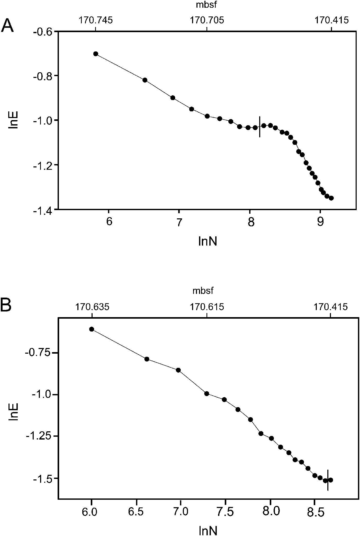
Using the Thomas (Reference Thomas, Wing, Gingerich, Schmitz and Thomas2003) high-resolution data as both single samples (SSA) and replicates over time (CFF), from oldest to youngest, biofacies or communities were defined by clustering as well as examination of a cumulative logarithmic plot of evenness versus number of individuals (Hayek and Buzas Reference Hayek and Buzas2010). We identified the same two foraminiferal communities with both techniques (Fig. 1). We subjected the clusters to Discriminant analysis, and they proved to be two significantly different groupings (Fig. 1).
Standardized canonical coefficients were computed to quantify this separation of the two communities, FCOM1 and FCOM2. Positive maximal value was descriptive of Bulimina simplex, whereas the negative weighted maximum coefficient was for Spiroplectammina spectabilis (−21.319). The unstandardized function evaluated for the group means yielded centroids of 113.06 for FCOM1 and −66.51 for FCOM2, providing for 100% correct, though biased, post hoc and resampled classification.
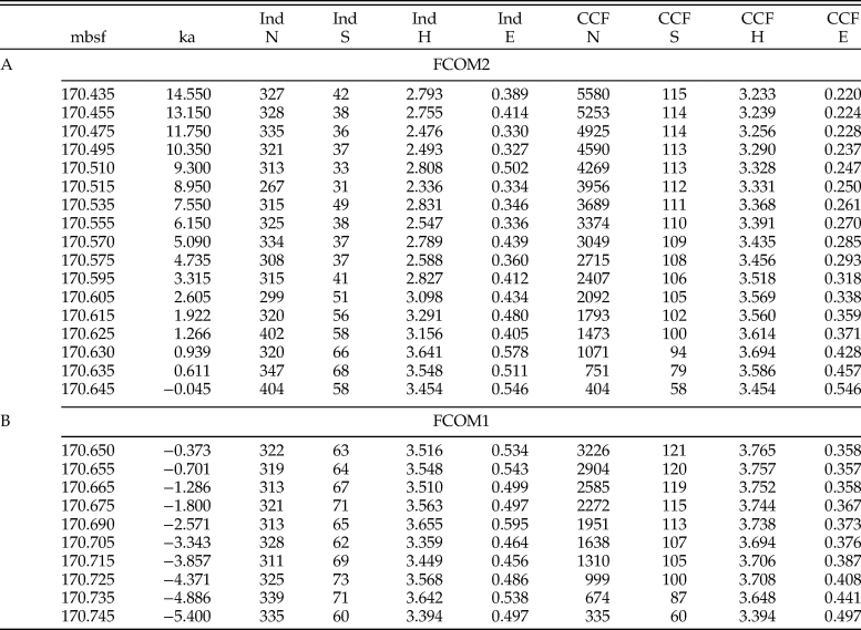
The first foraminiferal community, FCOM1, extends from 170.745 to 170.650 mbsf, (Table 1, Fig. 2), with the boundary between FCOM1 and FCOM2 at 170.650 mbsf, where Thomas (Reference Thomas, Wing, Gingerich, Schmitz and Thomas2003) indicated a marked increase in number of species. At 170.605 mbsf, Thomas (Reference Thomas, Wing, Gingerich, Schmitz and Thomas2003) recognized the strongest decline in species richness. The largest decrease in bulk sediment δ13C (Bains et al. Reference Bains, Corfield and Norris1999; Kirtland-Turner et al. Reference Kirtland-Turner, Hull and Ridgwell2017) is at 170.635 mbsf, within 2 cm of the boundary proposed here (Fig. 1).
A, Discrimination of FCOM1 by plot of lnE versus lnN. B, Discrimination of FCOM 2 by plot of lnE versus lnN. mbsf, meters below the seafloor.

Summary of both individual single-sample approach (SSA) samples and cumulative frequency function (CCF) values for FCOM1 and FCOM2. N = number of individuals; S = number of species; H = information function; and E = evenness for individual (Ind) and accumulated (CCF) samples in (B) FCOM1 and (A) FCOM2. mbsf, meters below sea floor; ka, in kyr before and after the carbon isotope excursion after Röhl et al. (Reference Röhl, Westerhold, Bralower and Zachos2007).

Figure 2 plots the 10 samples that compose FCOM1, the community that existed up to the disruptive event, using only the sample indices based upon individual samples. The independent variable is sample number or time, because the number of specimens (number counted) in each individual sample, N, is nearly constant (Table 1). Neither pictorially nor with regression analysis on these individual single samples is any trend apparent over the interval 170.745 to 170.650 mbsf (−5.40 to −0.373 kyr), and none of the regression coefficients are significantly different from zero. Examination of the values for the indices (Table 1, FCOM1) also shows no discernible trend. We conclude that the SSA, using individual samples, in FCOM1 indicate no perturbation.
Using the CFF method (Appendix) with samples over time and recalculating the indices at each stage provides a comprehensive picture of the species composition and their distribution within any community. The natural logarithms (ln) of these CFF values are plotted in Figure 3, while the numerical value of species (S) and distributional evenness (E) are shown in Table 1. For the data of FCOM1, the value of the diversity regression slope is 0.138 (Fig. 3), significantly different from 0 and positive.
Individual sample observations for lnS, H, and lnE versus sample number for foraminifera in FCOM1. Regression equations are:
 $${\rm lnS } = 4.215 - 0.00\,\;{\rm sample};{\rm AR}2 = 0.000;p = 0.654\;\quad$$
 $${\rm H } = 3.509 + 0.005\,\;{\rm sample};{\rm AR}2 = 0.000;p = 0.587\;\quad$$
 $${\rm lnE } = -0.720 + 0.008\,\;{\rm sample};{\rm AR2 } = 0.000;p = 0.387$$

Additionally, to compare and characterize this increasing slope as a departure from stasis for added interpretation of the perturbation, the logarithmic zero-slope distribution, that is, the theoretical model for stasis (Log series), was also plotted (Fig. 4). In the observed data, the first data point has an N = 335 and S = 60, whereas the last, or 10th observation in this FCOM1, has N = 3226 and S = 121 (Table 1). The last predicted S for the null model is 107. We have observed, therefore, 14 more species than expected from a baseline model of stasis. Figure 4 shows that the observed slope for lnE versus lnN is smaller than expected from the stasis model. FCOM1, the period up to the break between communities, thus represents a condition of low stress.
Observed accumulated data for lnS, H, and lnE versus lnN for foraminifera in FCOM1. Regression equations are:
Observations:
 $${\rm lnS } = 2.538 + 0.287{\rm lnN};{\rm AR}2 = 0.912;p = 0.000$$
 $$\;\;{\rm H } = 2.685 + 0.138{\rm lnN};{\rm AR}2 = 0.782;p = 0.000\;\;\;\;$$
 $${\rm lnE } = 0.147 - 0.149{\rm lnN};{\rm AR}2 = 0.971;p = 0.000$$
Stasis model:
 $${\rm lnS } = 2.608 + 0.256{\rm lnN}\qquad\qquad\qquad\qquad\qquad\;\;$$
 $$\;\;{\rm H } = 3.636 + 0.000{\rm lnN}\qquad\qquad\qquad\qquad\qquad\;\;\quad$$
 $${\rm lnE } = 1.028 - 0.256{\rm lnN}\qquad\qquad\qquad\qquad\qquad\;\;$$

We would not have detected this increasing diversity of the assemblage if we had examined the data with the usual SSA. Positive or increasing diversity of the dynamic community over the interval of FCOM1 thus can be recognized only by the CFF accumulation of samples over time and the inclusion of information on species composition and structure.
Seventeen of the remaining 19 samples in the Thomas (Reference Thomas, Wing, Gingerich, Schmitz and Thomas2003) data set (i.e., excluding these in FCOM1) constitute FCOM2, in the interval from 170.645 to 170.435 mbsf. The beginning of FCOM2 coincides with the initiation of the CIE (Fig. 1, Table 1). These 17 samples compose FCOM2, with the uppermost two samples of the 19 establishing the beginning of another new community of unknown duration. Table 1 allows an estimate of the duration of FCOM2, according to the age model in Röhl et al. (Reference Röhl, Westerhold, Bralower and Zachos2007). This community existed in a disrupted state for 14.595 kyr (i.e., from −0.373 to 14.55 kyr). Thus, the abrupt start of the CIE and the presumably related increase in temperature and other changing environmental conditions appear to have severely disrupted the foraminiferal community for approximately 15 kyr.
Figure 5 shows the SSA over the FCOM2 interval. Unlike in FCOM1, the regressions with sample number or time are each significant and negative. The individual values of S, H, and E decrease throughout the interval, as expected from the regression equations (Table 1). Figure 6 plots the natural logs of the indices using the CFF values for lnN, with the null model for stasis included for comparison. For FCOM2, the values of diversity, as described by H, decrease as sample size increases. Such a decrease can occur in a dynamically changing system, but in FCOM2 the values of evenness decrease at a fast rate, and the diversity slope is significantly negative, portraying a pattern of decreasing diversity coupled with increasing dominance. We interpret this perturbation as a period of ecological stress.
Individual sample observations for lnS, H, and lnE versus sample number for foraminifera in FCOM2. Regression equations are:
 $${\rm lnS } = 4.525 - 0.039\;\;{\rm sample};{\rm AR}2 = 0.594;p = 0.000$$
 $$\;\;{\rm H } = 4.090 - 0.062\;\;{\rm sample};{\rm AR}2 = 0.613;p = 0.000\;\;\;\;$$
 $${\rm lnE } = 0.434 - 0.024\;\;{\rm sample};{\rm AR}2 = 0.376;p = 0.005$$

Observed accumulated data for lnS, H, and lnE versus lnN for foraminifera in FCOM2.
Regression equations are:
Observations:
 $${\rm lnS } = {\rm }2.928{\rm } + {\rm }0.218{\rm lnN};{\rm AR}2{\rm } = {\rm }0.846;p = {\rm }0.000$$
 $$\;\;{\rm H } = {\rm }4.574{\rm }-{\rm }0.146{\rm lnN};{\rm AR}2{\rm } = {\rm }0.524;p = {\rm }0.000\quad\;$$
 $${\rm lnE } = {\rm }1.646{\rm }-{\rm }0.364{\rm lnN};{\rm AR}2{\rm } = {\rm }0.984;p = {\rm }0.000$$
Stasis model:
 $${\rm lnS } = {\rm }2.682{\rm } + {\rm }0.230{\rm lnN}\qquad\qquad\qquad\qquad\qquad$$
 $$\;\;\;\;{\rm H } = {\rm }3.498{\rm } + {\rm }0.000{\rm lnN}\qquad\qquad\qquad\qquad\qquad\;\;\quad$$
 $${\rm lnE } = {\rm }0.816{\rm }\ndash {\rm }0.230{\rm lnN}\qquad\qquad\qquad\qquad\qquad$$

The evenness is much lower in FCOM2 than in FCOM1 at similar values of N. For example, in FCOM1 at N = 3226, evenness is 0.358, while in FCOM2 at N = 3049, evenness is 0.285, a 20% decrease (Table 1). In FCOM2, the slope for the evenness regression is significantly different from 0, and the magnitude larger than that for the richness regression, resulting in a value of −0.146 for the slope of H, our diversity measure. The significant negative slope of the diversity equation might suggest that richness has reached an asymptote, that is, that no more new species can be observed, but this is not the case. Richness continues to increase throughout the entirety of FCOM2, from 58 to 115 (Table 1). The first sample in FCOM2 with N = 404 has S = 58 whereas the last has N = 5580 with S = 115. For N = 404 and S = 58, the diversity index α = 18.558, and at N = 5580 for this same value of N, we would expect S = 106 if the state of stasis existed. The observed S is about 9% greater than expected.
Comparison of Figures 3 and 5 shows that richness decreased with time when using only the SSA, but the total number of species obtained increases throughout the entire sampling time (Fig. 6). In other words, examination of each sample as part of the entire community, taking into account not only the number of species but also species composition, indicates that new species are encountered throughout the interval, as conditions became more variable, even while the total number of species in each sample is decreasing.
The total number of species in these foraminiferal samples was 134. In FCOM1 there are 121 species, so the number of species in FCOM2 that are not in FCOM1 is 13 (134 − 121). In a similar fashion, 115 total species are in FCOM2, so that 19 (134 − 115) species in FCOM1 are not in FCOM2. The number of species from FCOM1 not surviving into the FCOM2 period is then 19/121 = 16%. If the boundary is moved to 170.605, where Thomas (Reference Thomas, Wing, Gingerich, Schmitz and Thomas2003) placed it, then 35 species did not survive, and there was a decrease of 35/121 = 29%.
We summarize the results using whole number equivalents instead of natural logs, and include the B-P index, the percentage of the most abundant species (Table 2). The results show a decrease in diversity and increase in dominance, or equivalently, lower evenness, between the two communities. Not only does the percentage of the most dominant species increase between communities, but the dominant species themselves also change. In FCOM1 the most abundant species is Bulimina thanetensis, whereas in FCOM2 the most abundant species is Siphogenerinoides cf. brevispinosa.
Summary of measures for communities FCOM1 and FCOM2. n = number of samples; N = number of individuals; S = number of species; eH = e to H power; E = evenness; β1H = regression coefficient for H versus lnN; max% = % of most abundant species; S+ = number of species added; S− = number of species lost; Stotal = total species in both communities.

Total Foraminiferal Assemblage Turnover
Based upon the SSA, the average number of species in the FCOM1 samples is 66.5, for FCOM2 it is 44.8, so that the percentage decrease of species richness per sample from FCOM1 to FCOM2 is −33%. The mean assemblage turnover ATI between FCOM1 and FCOM2 for benthic foraminifera is 0.626, or about 63% change in the foraminiferal assemblage over the initiation of the PETM. The ATI calculated between FCOM1 and the first sample from FCOM2 showed 0.764 or approximately 76% change, while the comparison between the entirety of FCOM1 and FCOM2 resulted in ATI = −0.951, or about a 95% change or difference.
Siphogenerinoides cf. brevispinosa provided approximately 17% of this total change pre and post the start of the PETM period as shown by CoBBI, changing from a relative abundance of approximately 5.5% pre-PETM to 21.3% after. Abyssamina quadrata comprised 5.1%, Bolivinoides cf. decoratus, 6.8%, Bulimina kugleri, 5.8%, Bulimina thanetensis, 7.4%, Nuttallides truempyi, 5.1%, and Tappanina selmensis, 5.8%.
Discussion
We present a stand-alone method, perturbation detection analysis, or PDA, for detecting perturbations to an overall faunal assemblage. The PDA is the quantitative analogue of the qualitative basis in DiMichele et al. (Reference DiMichele, Behrensmeyer, Olszewski, Labandeira, Pandolfi, Wing and Bobe2004).
The PDA relies on the use of paleontological samples in a CFF form as replicates over time. This accumulation of samples is available in a variety of packages such as Past, Primer, or Pisces and is easily programmed into Excel. The SSA to community analysis, while widely used in the literature, cannot detect disruptions to assemblage patterns such as those resulting from increasing or decreasing diversity over time.
With the methodological approach of PDA, we show that each of the two biofacies (FCOM1 and FCOM2) can be examined with precise criteria for patterns of change or disruption. We could determine when total communities changed relative to the CIE at the start of the PETM. Late Paleocene FCOM1, with a positive diversity regression slope of + 0.138, was in a state of growth, which was not recognizable using the traditional SSA plot, and thus there were no indications of decline in richness before the sudden disruption. We can assume, then, that the initial environmental changes in the latest Paleocene provided for a positive community response, that is, increased diversity.
At −0.373 kyr, the environment changed sufficiently so that a new foraminiferal community, FCOM2, was established (Fig. 2B). The CFF of this second foraminiferal community (FCOM2) presents a striking contrast to that of community FCOM1, with approximately 76% turnover between the two communities. For FCOM2 the diversity slope is −0.146 (Table 1), indicating a significant disruption to the community right after the initial spike in the CIE. We were able to identify which species were at the forefront of that change, showing that the dominant species changed over the boundary of the perturbation event, from B. thanetensis to S. cf brevispinosa, with the percentage of the most dominant species increasing as another indicator of community stress. We also determined how long this state of disruptive community deterioration maintained, that is, ~15 kyr.
CoBBI showed that the relative abundance of S. cf. brevispinosa increased from 5.5% of the community to 21.3%. The number of species per sample decreases by 32% (Fig. 4) from a mean number of species of 66 in FCOM1 to 45 in FCOM2. The total number of species in FCOM1 = 121 and in FCOM2 = 115, a decrease of 5%, and species in the time period of FCOM2 are physically smaller (Thomas Reference Thomas, Aubry, Lucas and Berggren1998, Reference Thomas, Wing, Gingerich, Schmitz and Thomas2003; Foster et al. Reference Foster, Schmidt, Thomas, Arndt and Ridgwell2013; Schmidt et al. Reference Schmidt, Thomas, Authier, Saunders and Ridgwell2018). Species represented by double digits in FCOM1 became rarer and occurred only in single digits in some samples in FCOM2. Although present in the community, species do not appear in every sample, so the number of species is lower per sample in FCOM2.
Our results can be used alone or in combination with the null model of stasis (Buzas et al. Reference Buzas, Hayek, Buzas-Stephens and Simms2017) for a further interpretation and a quantitative examination of any dynamic faunal system and its changing patterns. By so doing, we can gain added information, broader interpretation, and stronger conclusions. The PDA is built upon the diversity component H and its regression, and the exact relationship between H, species richness, and evenness (Hayek and Buzas Reference Hayek and Buzas2010), has been established. A log-linear relationship between diversity components and the number of individuals defines community status: when a community is in stasis, the expected number of species for a given number of individuals is constant. However, the species composition of each sample will change slightly, because rare, and even some common, species will not appear in all samples (observed data are then probabilistically constant). A Log series distribution serves as a null model describing this situation (Hayek and Buzas Reference Hayek and Buzas2010), because its regression coefficient is 0 for diversity H versus lnN. This, in turn, requires the regression coefficients for lnS and lnE to be equal but of opposite sign (Hayek and Buzas Reference Hayek and Buzas2010). When the slope of H versus lnN is 0, there is an ecological balance between richness and evenness. We can therefore, with confidence, define stasis, or the ecological balance of nature, as equilibrium between species richness (S) and evenness (E), such that diversity (H) remains constant with space and/or time (Buzas et al. Reference Buzas, Hayek, Buzas-Stephens and Simms2017).
PDA thus can be used to detect perturbations or disruptions to the structure, composition, and diversity of any community and provides a mechanism to examine this disruption as deviation from the steady state of stasis and an in-depth interpretation in terms of the richness and evenness. Three types of disruption are recognizable by using PDA: (1) formation of a new community; (2) within-community growth; and (3) within-community decline. PDA allows us to see a new community as defined in terms of species composition and/or relative abundance. When community growth occurs, the regression coefficient for lnS versus lnN is greater than that for lnE versus lnN, so that the regression coefficient for H versus lnN will be positive. When there is serious community decline, the regression coefficient for lnE versus lnN is greater than that for lnS versus lnN and the regression coefficient for H versus lnN will be negative. On a log scale, neither growth nor decline is possible for extended periods. Continued community growth leads to an impossible increase in the number of species, whereas community decline can lead to the extinction of the community. We regard both disruptive states as temporary, potentially limiting perturbations leading back to eventual stasis.
In the deep sea (>1500 m depth), living benthic foraminifera exhibit stasis on a global basis, while stations close to the area of this study, in the Weddell Sea (Mackensen et al. Reference Mackensen, Grobe, Kuhn and Fütterer1990; Buzas et al. Reference Buzas, Hayek, Culver, Hayward and Osterman2014; Fig. 2), also exhibit stasis. Our expectation or hypothesis, then, is that we will see stasis at Site 690 in past communities. The Log series distribution is a simple one-parameter distribution, and a community exhibiting such a simple distribution most likely was limited by few environmental variables (May Reference May, Cody and Diamond1975). This is in agreement with the suggestion that either food and/or oxygen are the limiting variables in the deep sea (e.g., Bernhard Reference Bernhard1986, Reference Bernhard1992; Gooday Reference Gooday1988; Corliss and Emerson Reference Corliss and Emerson1990; Mackensen et al. Reference Mackensen, Grobe, Kuhn and Fütterer1990; Murray Reference Murray2001; Loubere Reference Loubere1994; Jorissen et al. Reference Jorissen, de Stigter and Widmark1995, Reference Jorissen, Fontanier, Thomas, Hillaire-Marcel and de Vernal2007; Schmiedl Reference Schmiedl1995).
A sample-by-sample SSA plot of the FCOM1 before the CIE indicates no difference in diversity H, S, or E with time, as expected with stasis (Fig. 2A), whereas the CFF plot shows clearly that there is no stasis (Figs. 3 and 4): lnS and H increased at a higher rate and lnE at a lower rate than expected from the null model for stasis. FCOM1 has a positive regression coefficient for diversity (Table 1), and thus was in a growth stage; FCOM2 shows a large decrease in evenness and a large increase in dominance relative to FCOM1 (Table 2). This steady decline and departure from stasis suggests that considerable variation occurred in the environment, such that community adaptation to a position of stasis was impossible.
Consequently, it does not seem likely that a simple change in food availability or oxygen levels alone could have been responsible for the continual decline in FCOM2. Suggestions and speculations of a decoupling between surface water productivity and food arrival at the bottom, changes in oxygen availability, abundance and types of food supply (including chemo-autotrophic primary producers), increasing corrosivity of deep water, and perhaps other factors may all have exerted influence (Thomas Reference Thomas, Wing, Gingerich, Schmitz and Thomas2003; Alegret et al. Reference Alegret, Ortiz, Arenillas and Molina2010; Schmidt et al. Reference Schmidt, Thomas, Authier, Saunders and Ridgwell2018). Our analysis suggests that continual environmental variability prevented the foraminiferal community of FCOM2 from achieving stasis for about 15 kyr and yet was not large enough to terminate FCOM2 and necessitate the establishment a new community. This only occurred with the last two samples, when a new community of indeterminate duration formed.
The use of high-resolution data is not a requirement for PDA. What is the vital issue in the PDA methodology is that the data be representative of the problem or time period of interest. With samples collected at, for example, 20 m intervals, we well might not have seen the crucial events of interest of our study period. Key events for investigation of community status with PDA across other time periods could include, for example, transgression–regression changes, extinction events of either fast or slow duration, or climate-related changes in present-day data. Predictive use of this methodology is possible with appropriate data: investigation of community status as conditions change through time either with paleobiological data or recent data on threatened species, including human populations, with current climate change events.
Conclusions
We present a novel stand-alone approach, perturbation detection analysis, or PDA, which can be used to dissect and analyze holistic community disruption as growth or decline over time, allowing identification of perturbation of entire communities and recognition of both positive increase and negative deterioration of the community.
We show that single samples for analytical purposes, SSA, are inadequate to address questions of disruptive event identification and disruptions from stasis.
We used data on benthic foraminifera in a high-resolution set of samples across the initiation of the PETM at Site 690 (Weddell Sea), a time of documented benthic foraminiferal extinction. We show that there were two perturbated communities of interest. The community before the PETM was in a growth stage, then terminated. The community that formed in the earliest PETM was in serious decline for ~15 kyr. We identified individual species changes over this boundary and within and between both communities, and this information on foraminiferal communities had not been seen before our use of PDA, a holistic approach to detecting perturbation.
Acknowledgments
We wish to thank J. Jett for all the work she has done and invaluable assistance she has provided to prepare plots, save us from computer glitches, and submit the article. We also wish to acknowledge the anonymous reviewers and L. Collins, the associate editor, for invaluable suggestions in improving the presentation of this work. E.T. recognizes funding through National Science Foundation award OCE 1536611.
Appendix
I. The Single-Sample Approach (SSA)
This is the traditional, commonly applied method used for data analysis of paleontological samples. The raw data, or counts for N and S per sample, are collected and inserted into a spreadsheet with species as column headings and rows as sample observed values. Then, relative abundances are calculated from these counts over samples by dividing by totals. This matrix or spreadsheet of relative abundances becomes the basis for all calculations when using single samples. This matrix of values also constitutes the statistical frequency data or statistical frequency function, f(x).
Used as single samples, even though inserted into an Excel spreadsheet or matrix, the individual samples give no indication of the structure, changes, or interactions of the assemblage, only of its composition, that is, which species are there and how many of each there are.
II. Distribution Function versus Frequency Function
Herein we shall use the statistical distribution function (also called the cumulative distribution function or cumulative frequency function) form of the sample data. This method of summing the samples (or integration) will be called CFF. The CFF is defined as
 $${\rm F}\lpar x \rpar = \int _0^x ^{}f\lpar s \rpar ds$$
where s is a dummy variable to show that the integration of the frequency function, f(s), is over all species, 0 to the largest number. F(x) is then the area under the curve up to the count x. The total area is 1 if the observations used are relative frequencies when integrated −∞ to +∞, or, over the entire population. F(x) describes the range of possible values that can be attained under accumulation and the probability that the value of the random variable is within some range of values. Use of the CFF makes sense for either continuous or discrete random variables, because it completely determines the distribution of random variable X. If we use discrete data such as our sample counts for a select number of species we can write:
 $$\; \; {\rm F}\lpar x \rpar = \sum ^0_x f\lpar s \rpar$$
The x-axis is the range of allowable values (or domain) for the function. If y is a count, it can range through the positive integers, while if y is a probability, it must fall between 0 and 1.
Consider the cumulative curve, where y = 0% to 100%, or the additive counts of new species accumulated over samples in the assemblage, and x = 0% to 100%, or the numbers of new individuals obtained in each step up to the total N. Each point on this curve then can be read as the number of individuals x that account for y percent or y number of the total. The steeper the slope of any given segment, the greater the degree of concentration in the total assemblage, all else being equal. The sum of the squared proportions can be derived as the weighted average slope of the cumulative curve.
Thus, to use this CFF method, we merely use the number of species observed in the first sample of the raw data as the starting point, then the next x value becomes the added number of new species observed, and so on.
III. The PDA for Detecting Patterns of Community Disruption
Instead of the SSA, which relies upon the frequency function form of data, and the individual samples, we use here a PDA, which method relies upon the CFF form for assemblage data, for detection of perturbations/disturbances to any community over any geological time period. In this study of the PETM, we used high-resolution data (1–2 cm). However, this is not a requirement. The requirement on samples is neither mathematical nor statistical. The requirement is that the samples must be geological or paleontologically representative of fossils or individuals within the time period or area sampled. If, for example, the samples were collected 100,000 kyr apart, then the chance of detecting either cohesive communities or perturbations would be greatly reduced, and most probablybe nonexistent.
The Five Steps for the PDA
Step 1. Determine the biofacies based upon the relative abundances formed from the collected or observed data samples. Any method can be used. However, because clustering and Principal Component analyses are not probabilistic statistical test methods, it is wise to use the resulting groups from these methods as input to a Discriminant analysis to be assured of their significance.
Step 2. Using the relative abundance matrix for each separate biofacies, employ the CFF method to accumulate the samples. That is, after the first time-ordered sample yields its N and S, each new step in the process is obtained by accumulating sample by sample all newly observed or sampled species and individuals.
Step 3. Calculate the diversity index, that is, Shannon's H, at each step or row in the new matrices.
Step 4. Fit a linear regression model to the diversity data over each sample in each biofacies separately, using H versus lnN, and note the sign of the significant slope coefficient. Positive slope is positive change or increase. Negative slope indicates a community under stress and decreasing, possibly toward extinction.
Step 5. The ATI and CoBBI can be calculated to determine the species and their contributions to the boundary or break between communities as well as the composition of each community. The length of time of any disruptive event can also be calculated.
ATI and CoBBI Measures
To complete the total foraminiferal community evaluations for disruption, in our case near and across the PETM boundary, we used two measures. First we used the Hayek and Wilson (Reference Hayek and Wilson2013) total ATI , which is applicable to the entire species assemblage (ATI) over each biofacies. The ATI procedure, though coupled with a quality control process approach, was applied to the benthic foraminifera from the Pleistocene on Blake Ridge (ODP Hole 994C) and Demerara Rise (ODP Hole 1261A) (Wilson and Hayek Reference Wilson and Hayek2015). These authors designated all assemblage change above a control limit as meaningfully elevated taxonomic assemblage change against background noise. For any set of stratigraphic samples, the ATI between each pair of adjacent samples is calculated as: ATIs = ∑ │p i 2 − p i 1│, which is the between-sample assemblage turnover, where the p ij, j = 1, 2 are the proportional abundances of the ith species in the jth ordered sample. The absolute value is used in this formula to quantify total amount of change. Without this absolute value, these differences, being both positive and negative, will always sum to zero. Calculations for ATI and the associated individual species contributions can be done on a total basis, a sample-by-sample basis, a biofacies basis, or a boundary sample to biofacies basis up a section. Hayek and Adey (Reference Hayek, Adey and Dar2012) developed a separate but related index, CoBBI, to identify those species in the assemblage that provided any proportional contribution to the total community change that occurred across biofacies boundaries, which we employ here. These are not the relative proportions from the observed sample but are determined uniquely for each boundary. This index is defined to be: CoBBI = │p i2 − p i1│/ATI, where the p ij are defined as above. We use the ATI in this calculation to examine the change at the community boundaries only. Use of these measures provides a systematic way to examine individual taxa within assemblages/biofacies/communities, as well as entire communities simultaneously.
IV. PDA, Evenness, and Richness: Disruptions from a Steady-State System
The PDA is a stand-alone method. However, it can also be used or shown as integrated into the approach of Buzas et al. (Reference Buzas, Hayek, Buzas-Stephens and Simms2017) with the five steps here for additional interpretation and inference.
The basis of these authors’ quantitative definition of stasis is the recognizable balance that can exist between evenness and richness when we consider the diversity of any assemblage either in space or in time. This balance is defined functionally with the well-known diversity decomposition equation (Hayek and Buzas Reference Hayek and Buzas2010). That is, H = lnS + lnE, where H is the Shannon index of diversity, S is species richness, and E is distributional evenness. Because these quantities on either side of the equals sign are equivalent, we can regress each component.
The value of the slope of diversity H against lnN used in our PDA can also be determined from the coefficients of the regressions of lnS versus lnN and lnE versus lnN. When the regression coefficient for S is greater than the regression coefficient for E, then the diversity regression coefficient (for H vs. lnN) will be positive. When the regression coefficient for S is smaller than that for E, the diversity regression slope will be negative.
Therefore, the diversity regression equation can be written as: β0H + β1H lnN and interpreted as a measure of the ecological balance of the community. In Buzas et al. (Reference Buzas, Hayek, Buzas-Stephens and Simms2017), we called the coefficient β1H the “relative abundance distribution index,” or RADI. However, we do not use that term here, because the elements of the matrix are calculated with the CFF procedure. This diversity regression represents a probabilistic constant state, or steady-state system, in which diversity is constant but requires a series of small inputs and outputs or changes in both richness and evenness to maintain. Therefore, this ecological system is dynamic and, when in balance, is in stasis. The Log series is used as a benchmark null model to describe this ecological balance between richness and evenness in nature, exhibited as community stasis, temporal or spatial stability (Hubbell Reference Hubbell2001; Hayek and Buzas Reference Hayek and Buzas2010). This distribution functions is the null model for stasis or balance, because in practice it will show a nonsignificant diversity slope of probabilistic 0 (under test, the slope cannot be distinguished from 0). Statistically, this nonsignificant slope value corresponds to the balance of evenness and richness in the community.
Then, we compare the actual numerical value of the diversity slope from the PDA. However, in this case, the diversity slope also equals the sum of the slopes for richness and evenness. Just as above, our PDA still detects perturbations or disruptions from this comparison resulting from stress to the community/assemblage and subsequently will result in a significantly negative slope. The alternative, when a community is increasing in species richness and diversity, or thriving, will result in an imbalance evidenced by a significantly positive slope. Using this as a complete system of stasis and disruptions to this steady state or balance provides for additional interpretation and community description. Once the states of stasis or disruption are determined, the length of time that such states were in existence can easily be calculated.