1 Introduction
The need for simplified models of subsonic turbulent jets and the sound they produce was in the past driven primarily by the need for low cost prediction and design guidance tools. In such a context, statistical, frequency-domain models are sufficient. More recent interest in closed-loop flow control motivates the search for time-domain models. In either case, the crux of the problem is to understand the underlying mechanisms such that the Navier–Stokes equations can be distilled down to some simplified form that captures these with accuracy sufficient for the job at hand.
One of the principal difficulties in applying linear control theory to fluidic systems relates to the high dimensionality of most flows and their nonlinear behaviour, in particular for turbulent cases, for which a high discretisation may be required to resolve the system accurately (Kim & Bewley Reference Kim and Bewley2007), the flow variables at each grid point being regarded as a state variable.
A possible strategy for coping with such difficulties involves constructing a reduced-order model of the system, for which linear control laws can be derived and tested a posteriori on a nonlinear simulation (i.e. direct numerical simulation or large-eddy simulation) or on an experiment (Belson et al. Reference Belson, Semeraro, Rowley and Henningson2013; Semeraro et al. Reference Semeraro, Bagheri, Brandt and Henningson2013; Fabbiane et al. Reference Fabbiane, Simon, Fischer, Grundmann, Bagheri and Henningson2015). The challenge is to obtain a reduced-order model that is both, computationally inexpensive and accurate in capturing the relationship between inputs and outputs of the system.
A promising paradigm for obtaining simplified description of the most acoustically relevant dynamics of turbulent jets involves linearisation of the Navier–Stokes equations about a time-averaged base flow. Solutions of such linearised equations for turbulent jets have been shown to provide a good description of coherent structures observed in data, and which are referred to as wavepackets (Suzuki & Colonius Reference Suzuki and Colonius2006; Gudmundsson & Colonius Reference Gudmundsson and Colonius2011; Cavalieri et al.
Reference Cavalieri, Rodríguez, Jordan, Colonius and Gervais2013; Jordan & Colonius Reference Jordan and Colonius2013), such a linearised system neglects explicit nonlinear interactions between the wavepackets and turbulence, which may occur via Reynolds stresses associated with the energy containing turbulent eddies (Crighton & Gaster Reference Crighton and Gaster1976). This simplified model has been shown to describe with reasonable accuracy the amplitudes and phases of wavepackets (linear hydrodynamic instabilities) (Cavalieri et al.
Reference Cavalieri, Rodríguez, Jordan, Colonius and Gervais2013; Jordan & Colonius Reference Jordan and Colonius2013): for the Strouhal number range
 $0.3<St<0.9$
and azimuthal modes
 $m=0$
and
 $m=1$
(which dominate the radiated sound field at low emission angles as observed by Cavalieri et al. (Reference Cavalieri, Jordan, Colonius and Gervais2012)), the averaged amplitudes and phases of harmonic wavepackets can be reproduced with good fidelity. More recently, predictions obtained from wavepacket models have been extended to
 $St$
up to 4.0 and azimuthal wavenumbers ranging from 0 to 4, via comparisons of results of the parabolised stability equations (PSE) and a large-eddy simulation of a Mach 0.9 turbulent jet (Cavalieri et al.
Reference Cavalieri, Sasaki, Schmidt, Colonius, Jordan and Bres2016).
In addition to round subsonic jets, linear wavepacket models have been used in the study of coaxial (Léon & Brazier Reference Léon and Brazier2011; Gloor, Obrist & Kleiser Reference Gloor, Obrist and Kleiser2013) and supersonic jets (Malik & Chang Reference Malik and Chang2000; Ray & Lele Reference Ray and Lele2007; Nichols & Lele Reference Nichols and Lele2011; Sinha et al. Reference Sinha, Rodríguez, Brès and Colonius2014). For the latter, wavepacket models may be readily extended to predict the acoustic field and lead to Mach wave radiation. Sinha et al. (Reference Sinha, Rodríguez, Brès and Colonius2014) compared wavepacket model predictions against results of large-eddy simulations and presented encouraging results for the peak far-field radiation.
For the subsonic case, however, sound radiation is more subtle, depending on characteristics of the amplitude envelope (Crighton & Huerre Reference Crighton and Huerre1990) and on the two-point coherence (Cavalieri & Agarwal Reference Cavalieri and Agarwal2014). Nevertheless, it is known that a correlation holds between the wavepackets in the hydrodynamic field and the resulting acoustic far-field emanating from a turbulent jet (Cavalieri et al. Reference Cavalieri, Rodríguez, Jordan, Colonius and Gervais2013). The two-point coherence plays an essential role where the acoustic efficiency of wavepackets is concerned, as shown by the coherence-matched linear source models studied by Reba, Narayanan & Colonius (Reference Reba, Narayanan and Colonius2010), Baqui et al. (Reference Baqui, Agarwal, Cavalieri and Sinayoko2013, Reference Baqui, Agarwal, Cavalieri and Sinayoko2015).
The works cited above focus primarily on the frequency-domain characteristics of wavepackets and their ability to reproduce statistical quantities of the flow variables, such as their power spectral densities (PSDs). In the context of closed-loop control however, such frequency-domain characteristics do not suffice, and we need a model capable of predicting, based on some measurement of the flow, the future evolution of wavepackets. To the best of the authors’ knowledge, prior to this work, such a model has never been obtained from linear (PSE), and it is unclear a priori whether such a model would be accurate for a high Reynolds jet, as the wavepackets are not harmonic, and are driven by the flow inside the nozzle, where the boundary layer is already turbulent.
The challenge, therefore, is to use unsteady data from sensors situated somewhere near the nozzle exit to predict the downstream evolution of wavepackets. Equipped with knowledge of how the flow will evolve, suitably positioned actuators can then be used to introduce perturbations, according to a control law, that would modify the wavepacket evolution in some desired way. The fast characteristic time scales of high-speed turbulent jets impose a considerable constraint in terms of the allowable computational cost of the predictive model, and the work described here addresses this issue: we are interested in developing fast-but-accurate prediction capabilities such that an estimation of the future state of the flow be feasible in real time in an experimental setting.
In the present work we propose a theoretical approach to construct a time-domain model for wavepackets in turbulent jets. This is motivated by, and indeed derived from, the frequency-domain model evoked above; the linear parabolised stability equations are used on account of their low computational cost. The modelling involves two steps. First a frequency-domain transfer function, between a single upstream station and many downstream stations, is derived from the PSE. This is then inverse Fourier transformed in order to recover its time-domain counterpart. Near-field pressure measurements in the vicinity of the exit plane convolved with the transfer function allows estimation of the entire downstream evolution of the flow: all dependent variables can be predicted with the model, in real time and over an extensive spatial grid. In this sense the model is single-input–multiple-output (SIMO).
Two other possibilities are also studied here, providing single-input–single-output (SISO), models based on the near-field pressure measurements of Breakey et al. (Reference Breakey, Jordan, Cavalieri, Léon, Zhang, Lehnasch, Colonius and Rodriguez2013). The first involves an autoregressive moving-average exogenous (ARMAX) system identification to provide a transfer function between upstream and downstream measurements. The second approach involves direct measurement of empirical transfer functions from the same measurements, using the cross-spectral density between an upstream sensor and a downstream position where a flow variable is estimated. The two methods require measurement of fluctuating flow quantities.
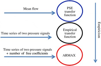
The performance of the theoretical time-domain model is compared with those of the ARMAX model and the empirical transfer function. The three techniques form a hierarchy of methods (figure 1) for real-time, sensor-based, estimation of the evolution of wavepackets in turbulent jets, ranging from the most empirical (ARMAX) which is built from unsteady data, to the first-principles PSE model, which depends only on the turbulent mean and the linearised equations of motion.
The paper is organised as follows. In the next section the experiment is briefly described. This is followed, in § 3, by a presentation of the modelling methodologies. Section 4 goes on to present an evaluation of the performance of these. Some concluding remarks are provided in § 6.
Hierarchy of methods for real-time estimation, from first principles to the most empirical, with respective inputs.

2 Experimental set-up
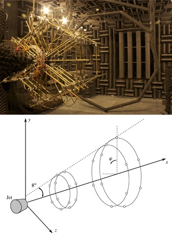
The experiments were carried out at the ‘Bruit and Vent’ (figure 2) anechoic jet-noise facility of the Institut Pprime, Poitiers, France. An unforced, Mach
 $M=0.6$
jet, issuing from a 50 mm diameter nozzle, previously used in a number of other studies (Breakey et al.
Reference Breakey, Jordan, Cavalieri, Léon, Zhang, Lehnasch, Colonius and Rodriguez2013; Cavalieri et al.
Reference Cavalieri, Rodríguez, Jordan, Colonius and Gervais2013), was considered. The corresponding Reynolds number, based on the nozzle diameter, and the air density, viscosity and velocity at the nozzle exit, was
 $5.7\times 10^{5}$
. A carburundum trip placed
 $2.7$
diameters upstream of the nozzle lip was used to ensure that the boundary layer be turbulent at the jet exit. The length of the potential core of this jet is between 5 and 5.5 diameters.
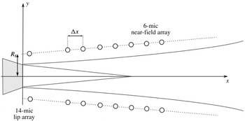
Pressure measurements were made in the jet near field (see figure 3) using a 42-microphone cage array comprising seven six-microphone rings that partially cover a conical surface of inclination angle
 $8^{\circ }$
following the jet divergence. This conical surface intersects the jet nozzle plane at a radial distance of
 $R_{s}=0.6$
or
 $0.8$
, depending on the configuration. Figure 2 shows schematically the positioning of the conical surface. The spacing between successive rings was
 $0.75D$
where
 $D$
is the diameter of the nozzle. This measurement configuration permits azimuthal Fourier series decomposition of the pressure field, providing real-time sensing of the space–time behaviour of azimuthal modes
 $m=0$
,
 $m=\pm 1$
and
 $m=\pm 2$
(as per (2.1)) over an extended axial region. The present work focus on azimuthal number
 $m=0$
, due to its importance for sound radiation in turbulent jets (Cavalieri et al.
Reference Cavalieri, Rodríguez, Jordan, Colonius and Gervais2013), but results for
 $m=1$
are also presented in the Appendix. Near the nozzle lip an additional ring array of 14 microphones was installed in order to investigate the relationship between the near-lip fluctuations of the flow and the downstream evolution.
A second campaign obtained data over a wider range of axial positions, ranging from
 $0.5D$
to
 $8.9D$
, with a finer resolution of
 $0.4D$
. An array of four six-microphone rings, each independently displaceable in the axial direction, was used. While the first campaign provided simultaneous measurement of the near-field pressure field, this experiment was designed to obtain fine-resolution measurement of the statistical properties of the jet fluctuations via a two-point correlation analysis. The two-point cross-spectral matrix (CSM) can be built and used in the application of proper orthogonal decomposition. All measurements were ensured to be on the same conical surface, with
 $R_{s}=0.8D$
, the radial positions of the microphones being adjusted each time a ring was moved axially. Each azimuthal mode is obtained via a standard Fourier series in azimuth, where
 $p$
is the pressure fluctuation,
 $x$
the streamwise position,
 $t$
time and
 $phi$
the azimuthal angle.
 $$\begin{eqnarray}\tilde{p}_{m}(x,t)=\tilde{p}(x,m,t)=\int _{0}^{2\unicode[STIX]{x03C0}}p^{\prime }(x,\unicode[STIX]{x1D719},t)\text{e}^{-\text{i}m\unicode[STIX]{x1D719}}\,\text{d}\unicode[STIX]{x1D719}.\end{eqnarray}$$
Wind tunnel facility ‘Bruit and Vent’ and scheme of the conical surface for positioning of the near-field microphones.

Experimental set-up: near-field microphone cage array in the seven-ring configuration.

3 Modelling methodologies
The hierarchy of approaches used to obtain real-time models are described in what follows.
3.1 Parabolised stability equations
The PSE represents an extension of the parallel flow linear stability problem to base flows with mild streamwise variation. The total flow field
 $\boldsymbol{q}$
is decomposed into a mean, time-averaged axisymmetric component
 $\overline{\boldsymbol{q}}(\boldsymbol{x})$
and a time-dependent fluctuation
 $\boldsymbol{q}^{\prime }(\boldsymbol{x},t)$
, where
 $\boldsymbol{q}=[u_{x},u_{r},u_{\unicode[STIX]{x1D703}},\unicode[STIX]{x1D70C},T]^{\text{T}}$
represents the flow variables (axial, radial and azimuthal components of velocity, density and temperature, respectively) and cylindrical coordinates
 $\boldsymbol{x}=[x,r,\unicode[STIX]{x1D703}]$
are being used.
Since the mean flow is homogeneous in the azimuthal direction and in time, the fluctuation may be expressed in terms of normal modes in these directions,
 $$\begin{eqnarray}\boldsymbol{q}^{\prime }(\boldsymbol{x},t)=\mathop{\sum }_{\unicode[STIX]{x1D714}}\mathop{\sum }_{m}\tilde{\boldsymbol{q}}(x,r)\text{e}^{\text{i}m\unicode[STIX]{x1D703}}\text{e}^{-\text{i}\unicode[STIX]{x1D714}t},\end{eqnarray}$$
where
 $\tilde{\boldsymbol{q}}$
is the complex-valued amplitude for frequency
 $\unicode[STIX]{x1D714}$
and azimuthal wavenumber
 $m$
.
One may further simplify the solution by decomposing
 $\tilde{\boldsymbol{q}}(x,r)$
into two separate contributions, a slowly varying function representing the amplitude envelope of the solution and a fast, oscillatory function that captures the wave-like axial structure. This solution corresponds to the wavepacket ansatz for slowly diverging jets (Crighton & Gaster Reference Crighton and Gaster1976) and allows parabolisation of the linearised equations,
 $$\begin{eqnarray}\boldsymbol{q}^{\prime }(\boldsymbol{x},t)=\hat{\boldsymbol{q}}(x,r)\exp \left(\text{i}\int ^{x}\unicode[STIX]{x1D6FC}(x^{\prime })\,\text{d}x^{\prime }\right)\text{e}^{\text{i}m\unicode[STIX]{x1D703}}\text{e}^{-\text{i}\unicode[STIX]{x1D714}t},\end{eqnarray}$$
where
 $\unicode[STIX]{x1D6FC}=\unicode[STIX]{x1D6FC}_{r}+\text{i}\unicode[STIX]{x1D6FC}_{i}$
is the complex-valued axial wavenumber, whose imaginary part is related to exponential growth or decay of disturbances in
 $x$
. Slow variations in
 $x$
are assumed for both
 $\hat{\boldsymbol{q}}$
and
 $\unicode[STIX]{x1D6FC}$
. The decomposition in (3.2) is based on a distinction between the slowly varying amplitude functions
 $\hat{\boldsymbol{q}}(x,r)$
and the fast changes associated with the
 $\unicode[STIX]{x1D6FC}$
integral.
On substitution of (3.2) into the linearised, compressible Euler, energy and continuity equations, a matrix system is obtained,
 $$\begin{eqnarray}(\unicode[STIX]{x1D63C}(\overline{\boldsymbol{q}})+\unicode[STIX]{x1D63D}(\overline{\boldsymbol{q}},\unicode[STIX]{x1D6FC},\unicode[STIX]{x1D714}))\hat{\boldsymbol{q}}+\unicode[STIX]{x1D63E}(\overline{\boldsymbol{q}})\frac{\unicode[STIX]{x2202}\hat{\boldsymbol{q}}}{\unicode[STIX]{x2202}x}+\unicode[STIX]{x1D63F}(\overline{\boldsymbol{q}})\frac{\unicode[STIX]{x2202}\hat{\boldsymbol{q}}}{\unicode[STIX]{x2202}r}=0,\end{eqnarray}$$
where the high Reynolds number of the flows considered justifies neglect of the viscous terms. Matrices
 $\unicode[STIX]{x1D63C}$
,
 $\unicode[STIX]{x1D63D}$
,
 $\unicode[STIX]{x1D63E}$
and
 $\unicode[STIX]{x1D63F}$
are linear operators, dependent on the base flow, wave number and frequency considered; their exact form may be found, for example, in Gudmundsson (Reference Gudmundsson2010). Details of the derivation may be found elsewhere (Herbert Reference Herbert1997; Gudmundsson & Colonius Reference Gudmundsson and Colonius2011; Sasaki Reference Sasaki2014). The linearity of the above system allows independent calculation of each
 $\unicode[STIX]{x1D714}-m$
combination, an ensemble of which is then used to construct a frequency-domain model, from which a transfer function between any two given positions in the jet can be derived.
The PSE system (3.3) requires a further condition, necessary to eliminate the ambiguity between
 $\hat{\boldsymbol{q}}$
and
 $\unicode[STIX]{x1D6FC}$
, since the spatial growth in the axial direction may be absorbed into either the shape function
 $\hat{\boldsymbol{q}}$
or the complex amplitude
 $\text{e}^{\text{i}\int \unicode[STIX]{x1D6FC}(x^{\prime })\,\text{d}x^{\prime }}$
. We follow the normalisation proposed in Herbert (Reference Herbert1997), which removes the exponential axial dependence of the shape functions by imposing,
 $$\begin{eqnarray}\int _{0}^{\infty }\hat{\boldsymbol{q}}\frac{\unicode[STIX]{x2202}\hat{\boldsymbol{q}}\ast }{\unicode[STIX]{x2202}x}r\,\text{d}r=0.\end{eqnarray}$$
Discretising (3.3) and (3.4) one obtains, via an iterative algorithm (Gudmundsson & Colonius Reference Gudmundsson and Colonius2011), a numerical solution for
 $\hat{\boldsymbol{q}}$
and
 $\unicode[STIX]{x1D6FC}$
. Further discussion on this procedure and on the PSE method in general can be found in the literature (Herbert Reference Herbert1997; Gudmundsson & Colonius Reference Gudmundsson and Colonius2011; Cavalieri et al.
Reference Cavalieri, Rodríguez, Jordan, Colonius and Gervais2013; Rodríguez et al.
Reference Rodríguez, Cavalieri, Colonius and Jordan2014; Sasaki Reference Sasaki2014).
3.1.1 Numerical methods
A pseudo-spectral method is used to discretise the functions in the radial direction by means of Chebyshev polynomials, whose spectral accuracy is desirable for solutions at high Strouhal number, which are necessary for construction of the transfer function. The axial derivatives are calculated using finite differences, and the spatial marching is performed using an implicit Euler method. A mapping function is used to transform the
 $[-1~1]$
Chebyshev domain to an infinite one. Dirichlet boundary conditions are imposed on the flow variables at
 $r\rightarrow \infty$
and the centreline conditions are dealt with using the procedure described by Mohseni & Colonius (Reference Mohseni and Colonius2000).
After spatial discretisation of the radial and axial directions and imposition of the boundary conditions, the system in (3.3) takes the form of the following initial value problem:
 $$\begin{eqnarray}(\unicode[STIX]{x0394}x(\unicode[STIX]{x1D63C}+\unicode[STIX]{x1D63D}+\unicode[STIX]{x1D63F}{\mathcal{D}}_{r})+\unicode[STIX]{x1D63E})^{j+1}\hat{\boldsymbol{q}}^{\,j+1}=\unicode[STIX]{x1D63E}^{j+1}\hat{\boldsymbol{q}}^{\,j},\end{eqnarray}$$
where
 ${\mathcal{D}}_{r}$
denotes the discrete radial derivative,
 $\unicode[STIX]{x0394}x$
is the streamwise spacing and spatial marching is realised to evolve the solution from
 $\unicode[STIX]{x0394}x_{j}$
to
 $\unicode[STIX]{x0394}x_{j+1}$
.
The solution of this problem requires initial conditions for the shape functions
 $\hat{\boldsymbol{q}}$
. These conditions are taken close to the nozzle exit, and are calculated by considering the parallel flow approximation
 $(\unicode[STIX]{x2202}\hat{\boldsymbol{q}}/\unicode[STIX]{x2202}x)=0$
, which allows for the definition of a spatial stability eigenvalue problem,
 $$\begin{eqnarray}\left(\unicode[STIX]{x1D63C}+\unicode[STIX]{x1D609}_{1}+\unicode[STIX]{x1D63F}\frac{\unicode[STIX]{x2202}}{\unicode[STIX]{x2202}r}\right)\hat{\boldsymbol{q}}=\unicode[STIX]{x1D6FC}(-\unicode[STIX]{x1D609}_{2})\hat{\boldsymbol{q}},\end{eqnarray}$$
where the
 $\unicode[STIX]{x1D63D}$
matrix is decomposed into
 $\unicode[STIX]{x1D609}_{1}+\unicode[STIX]{x1D6FC}\unicode[STIX]{x1D609}_{2}$
.
Since PSE is a linear method, the amplitude of the solution is undefined and it may be multiplied by a constant in order to fit the experimental data. As will be shown later for the transfer function approach, we work with the division of the output solution by the input which eliminates the need to determine the free constant.
Finally, the experimental data used to define the mean flow were fitted with a Gaussian profile as in Tam & Burton (Reference Tam and Burton1984), in order to avoid non-smoothness problems,
 $$\begin{eqnarray}\overline{u}=\left\{\begin{array}{@{}ll@{}}1\quad & \text{if}~r<R(x),\\ \displaystyle u_{c}(x)\exp \left[\frac{-(r-R(x))^{2}}{\unicode[STIX]{x1D6FF}^{2}(x)}\right],\quad & \text{otherwise},\end{array}\right.\end{eqnarray}$$
where the parameters
 $R(x)$
,
 $u_{c}(x)$
and
 $\unicode[STIX]{x1D6FF}(x)$
are determined from a least squares fit to the experimental data. The PSE code is the same used in Koenig et al. (Reference Koenig, Sasaki, Cavalieri, Jordan and Gervais2016), where the validation results obtained using the same flow studied in this work can be found.
3.1.2 SISO modelling using PSE
In this section, the linearity of PSE is exploited to obtain a SISO model between any two axially separated positions in a turbulent jet. Although the procedure is derived and validated using near-field pressure measurements – which is an easily available experimental quantity – it can be applied to any other dependent variable; indeed the input and output are not required to be the same variable.
In what follows
 $R(\unicode[STIX]{x1D714})$
denotes a quantity in the frequency domain, and
 $r(t)$
is the same quantity in the time domain; the two are related by the direct and inverse Fourier transform pair. Defining
 $R(\unicode[STIX]{x1D714})$
and
 $Y(\unicode[STIX]{x1D714})$
as the complex pressures at two axially and radially separated positions along the jet and assuming a linear relation between these, a frequency-domain transfer function can be obtained as,
 $$\begin{eqnarray}G(\unicode[STIX]{x1D714})=\frac{Y(\unicode[STIX]{x1D714})}{R(\unicode[STIX]{x1D714})}.\end{eqnarray}$$
A time-domain transfer function,
 $g(t)$
, is then available following an inverse Fourier transform,
 $$\begin{eqnarray}g(t)=\frac{1}{2\unicode[STIX]{x03C0}}\int _{-\infty }^{\infty }G(\unicode[STIX]{x1D714})\text{e}^{-\text{i}\unicode[STIX]{x1D714}t}\,\text{d}\unicode[STIX]{x1D714}.\end{eqnarray}$$
Once
 $g(t)$
is obtained, the output
 $y(t)$
of the system can be predicted by convolution with the input
 $r(t)$
and a SISO system is defined as:
 $$\begin{eqnarray}y(t)=\int _{0}^{\infty }g(\unicode[STIX]{x1D70F})r(t-\unicode[STIX]{x1D70F})\,\text{d}\unicode[STIX]{x1D70F}\end{eqnarray}$$
where
 $\unicode[STIX]{x1D70F}$
is an auxiliary variable, introduced only for performing the convolution integral. However, only the behaviour associated with linear PSE (i.e. linear wavepackets) is being predicted; as shown in earlier works (Cavalieri et al.
Reference Cavalieri, Rodríguez, Jordan, Colonius and Gervais2013), downstream of the potential core, the PSE model presents an early saturation when compared with actual experimental data and thus a deterioration of the prediction is expected in that region.
Implicit in this procedure is that a single mode dominates the dynamics between the positions of input and output, such that a single upstream sensor allows an estimation of the amplitudes and phases of this mode. The PSE transfer function can be seen as a propagator of this mode between the two positions. For the turbulent jets considered here, the dynamics at the near-nozzle region is dominated by the exponential growth of the Kelvin–Helmholtz mode, allowing thus the use of (3.10) to estimate an output from a single input in this region.
The convolution in (3.10) is an operation with low computational cost. Considering that
 $g(t)$
is previously determined, the convolution in (3.10) involves
 $n_{t}$
multiplications and sums, where
 $n_{t}$
is the number of time steps used to discretise (3.10). This reduced number of operations makes such an approach a candidate for implementation in experimental settings.
Equation (3.10) is only useful for real-time prediction of the flow behaviour when there is a causal relationship between input and output signals, which implies
 $g(t<0)=0$
. This is the case for convection-dominated flows, such as the cold jets studied in this work, if the output
 $y(t)$
is downstream of the input
 $r(t)$
. Indeed, the Kelvin–Helmholtz mode considered here has a positive generalised group velocity (Davis et al.
Reference Davis, Couder, Pedley, Huerre, Jimenez, Moffatt, Worster, Huppert, Garrett and Mcintyre2000), which should lead to causal transfer functions if one attempts to estimate the downstream behaviour from an upstream input.
PSE was thus used to calculate pressure fluctuations for the axisymmetric mode. The computation is repeated for many Strouhal numbers (the low computational cost of PSE makes this feasible), and a change of variables is necessary in order to perform the inverse Fourier transform:
 $$\begin{eqnarray}\text{d}\unicode[STIX]{x1D714}=2\unicode[STIX]{x03C0}\frac{U_{jet}}{D}\,\text{d}St,\end{eqnarray}$$
where
 $U_{jet}$
is the jet velocity and
 $St$
is the Strouhal number, defined as
 $St=f\ast D/U_{jet}$
. Using this definition the inverse transform is,
 $$\begin{eqnarray}g(t)=2\unicode[STIX]{x03C0}\frac{1}{2\unicode[STIX]{x03C0}}\frac{U_{jet}}{D}\int _{-\infty }^{\infty }G\left(\frac{U_{jet}}{D}St\right)\exp \left(-\text{i}\frac{U_{jet}}{D}St\cdot t\right)\,\text{d}St.\end{eqnarray}$$
Or, by defining
 $F^{-1}[G(\unicode[STIX]{x1D714})]$
as the inverse Fourier transform of
 $G(\unicode[STIX]{x1D714})$
:
 $$\begin{eqnarray}g(t)=2\unicode[STIX]{x03C0}\frac{U_{jet}}{D}F^{-1}\left[G\left(\frac{U_{jet}}{D}St\right)\right].\end{eqnarray}$$
Use of the scaling property of the Fourier transform gives,
 $$\begin{eqnarray}g\left(t\frac{U_{jet}}{D}2\unicode[STIX]{x03C0}\right)=F^{-1}[G(St)].\end{eqnarray}$$
Defining the non-dimensional time,
 $t^{\ast }=t(U_{jet}/D)$
, we have,
 $$\begin{eqnarray}g(2\unicode[STIX]{x03C0}t^{\ast })=F^{-1}[G(St)].\end{eqnarray}$$
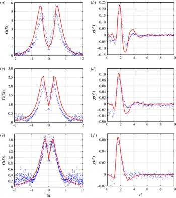
Frequency and time-domain transfer functions between three input–output combinations ((a,b:
 $x_{i}/D,x_{o}/D)=(0.05,1.7)$
; c,d:
 $(1.3,2.5)$
; e,f:
 $(2.1,3.3)$
) for pressure fluctuations on the
 $8^{\circ }$
conical surface. Blue dots: experimental data; solid red lines: PSE.

The frequency-domain transfer function
 $G(St)$
is obtained for each Strouhal number separately and is performed up to
 $St\approx 2.0$
, in intervals of 0.02. To ensure an appropriate time range, these frequency results are projected onto a finer grid of frequencies. This is realised by interpolating the amplitudes and phases of the PSE solution separately.
The PSE system has the property that the minimum marching step size (
 $\unicode[STIX]{x1D6FF}x$
) for convergence depends on the Strouhal number considered (Herbert Reference Herbert1997). The lower the frequency, the greater the value of
 $\unicode[STIX]{x1D6FF}x$
for convergence. This property may lead to difficulties for the low frequencies (
 $St\leqslant 0.2$
) and also to a mismatch between the axial grids used for each Strouhal calculation. These difficulties are dealt with by solving each frequency with its appropriate axial step and interpolating them to a finer axial grid. Such interpolation is also made by considering the amplitude and phase of the solution separately.
Figure 4 presents frequency and time-domain comparisons of the transfer functions obtained by PSE with those obtained experimentally (see the following subsection for a description of how the experimental transfer functions are computed). Three input–ouput combinations are shown for radial positions on the
 $8^{\circ }$
conical surface (cf. figure 3). The frequency-domain transfer functions present a peak around
 $St=0.3$
, where the comparison with experiment is most convincing (Cavalieri et al.
Reference Cavalieri, Rodríguez, Jordan, Colonius and Gervais2013). As the input is moved further downstream, the predicted output is underestimated. The time-domain model presents causal behaviour, as expected, for the input and output positions considered. Further evaluation of the performance of this method is presented in § 4 where it is compared with two other data-based techniques.
3.2 Empirical transfer function
The objective here is to realise a linear system identification, via the available unsteady measurements. An analogous procedure has been used by Dahan, Morgans & Lardeau (Reference Dahan, Morgans and Lardeau2012) to characterise the response of a flow to an actuation and to obtain a control law.
Based on the measured pressure data, with the hypothesis that a linear relation holds between the pressure field at two different axial locations along the jet, the optimal frequency response, in the least squares sense, may be defined from the auto- and cross-spectra of the input and output signals (Bendat & Piersol Reference Bendat and Piersol2011) as
 $$\begin{eqnarray}G(\unicode[STIX]{x1D714})=\frac{S_{ry}(\unicode[STIX]{x1D714})}{S_{rr}(\unicode[STIX]{x1D714})},\end{eqnarray}$$
where
 $S_{rr}$
and
 $S_{ry}$
are, respectively, the auto- and cross-spectra of the input and output signals. Inverse Fourier transform (3.9) of (3.16) provides an empirical, time-domain transfer function that can be used to estimate downstream evolution of the pressure field based on upstream measurements (3.10). To obtain the empirical transfer function, one should have the cross-spectral density between input and output, which in turn requires simultaneous measurements of the two quantities.
This approach can be considered a compromise between ARMAX system identification (which is described next) and the first-principles PSE transfer function in so far as it comprises an identification using unsteady data, but with a formulation consistent with the theoretical framework of linear PSE. The empirical transfer function is shown in figure 4 where it is compared with its PSE counterpart for three input–ouput pairs.
3.3 ARMAX system identification
The third approach, which also involves system identification, has been shown by Hervé et al. (Reference Hervé, Sipp, Schmid and Samuelides2012), using a numerical simulation of flow over backward-facing step, to be promising for amplifier-type flows.
The objective is again to build a SISO model. The identification is performed using an ARMAX, (the Matlab routine armax was used to perform the calculations), whose ansatz takes the form:
 $$\begin{eqnarray}\displaystyle & \displaystyle y(t)+\mathop{\sum }_{k=1}^{n_{a}}a_{k}y(t-k)=\mathop{\sum }_{k=n_{d}}^{n_{b}+n_{d}}b_{k}r(t-k)+E(t) & \displaystyle\end{eqnarray}$$
 $$\begin{eqnarray}\displaystyle & \displaystyle E(t)=\mathop{\sum }_{k=1}^{n_{c}}c_{k}e(t-k)+e(t), & \displaystyle\end{eqnarray}$$
where
 $y(t)$
is the simulated output value at time
 $t$
, given by an expression that includes an autoregressive part,
 $y(t-k)$
, an exogenous part represented by
 $r(t-k)$
, with
 $s$
the measured input to the system (sensor), and
 $a_{k}$
,
 $b_{k}$
and
 $c_{k}$
are linear coefficients. A moving-average term,
 $E(t)$
, accounts for phenomena that impact the measurement,
 $y$
, but are not observed by the sensor.
The identification works by means of a regression that seeks the coefficients
 $a_{k}$
,
 $b_{k}$
and
 $c_{k}$
that lead to a minimal-variance noise
 $e(t)$
. The model requires the parameters
 $n_{a}$
,
 $n_{d}$
,
 $n_{b}$
,
 $n_{c}$
, to be set and these can be related to certain properties of the flow, such as, the convection velocity of wavepackets and their characteristic length and time scales (Piantanida, Le Rallic & Jordan Reference Piantanida, Le Rallic and Jordan2014).
The coefficient
 $n_{a}$
represents the number of previous output data on which the current output depends. It is set by computing the autocorrelation function of the output signal. The parameter has been set as the temporal shift approximately corresponding to half of the first oscillation period of the correlation function.
The
 $n_{d}$
parameter indicates the temporal delay between the input and output signal; when different from
 $0$
, it implies that the effect of the input on the output is not instantaneous.
 $n_{b}$
represents the number of past input samples on which the current output depends. These two parameters may be obtained by considering the cross-correlation between
 $s$
and
 $y$
.
For the precise values of the parameters
 $n_{a}$
,
 $n_{d}$
,
 $n_{b}$
,
 $n_{c}$
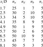
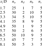
a sensitivity evaluation of the predicted output was assessed and will not be presented here for the sake of brevity. In what follows, the ARMAX results correspond to that of optimised values of these, as presented on table 1 for the considered output positions.
Optimised values of ARMAX parameters.
4 Results and discussion
4.1 Estimation from unfiltered near-field pressure
Transfer functions obtained using the three approaches described in the previous section were used to estimate the downstream evolution of wavepackets in the turbulent jet presented in § 2. Time series of the
 $m=0$
pressure signature at three upstream stations,
 $x/D=0.5$
,
 $1.3$
and
 $2.1$
, were convolved with the transfer functions to estimate the pressure field at a range of downstream positions.
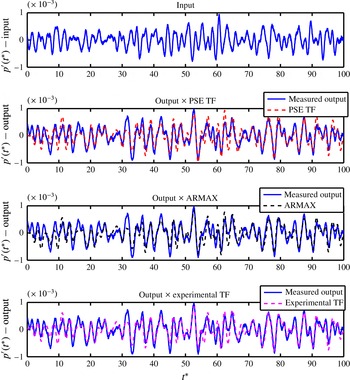
Comparison between measured non-dimensional pressure fluctuations, PSE transfer function, empirical transfer function and ARMAX predictions, with
 $x/D=2.1$
and
 $3.3$
as the input and output positions, respectively.

Figure 5, which presents some sample comparisons between estimation and measurement for
 $(x_{i}/D,x_{o}/D)=(2.1,3.3)$
, gives a sense of how well all three approaches can perform. The quantity shown is the non-dimensional pressure fluctuation,
 $p^{\prime }=(p/\unicode[STIX]{x1D70C}_{o}c_{0}^{2})$
(with
 $\unicode[STIX]{x1D70C}_{0}$
and
 $c_{0}$
the ambient density and sound velocity), plotted as a function of non-dimensional time.
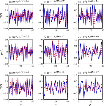
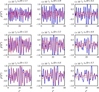
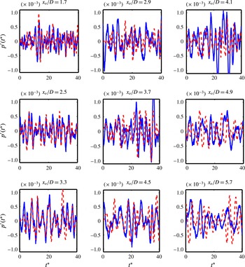
Figure 6 shows how estimation using the PSE transfer function performs as the output station is moved downstream. The precision gradually deteriorates, that of the amplitude more than that of the phases and characteristic frequencies. Similar trends are observed when the empirical transfer function and ARMAX model are used as estimation techniques. Given that we are considering a high Reynolds number turbulent jet issuing from a nozzle with a turbulent boundary layer, the performance of all three techniques is encouraging. The performance of the PSE model is, however, particularly promising, given that the only information necessary for its construction is the mean flow and the linearised equations of motion. This result constitutes a convincing demonstration of the reality of linear wavepackets in turbulent jets as real-time – as well as statistical, harmonic – entities.
Comparison between measured non-dimensional pressure fluctuations (solid line) and PSE transfer function prediction (dashed line) for
 $x/D=0.5$
,
 $1.3$
and
 $2.1$
, in the first, second and third lines, respectively.

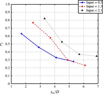
As a performance metric we use the normalised peak correlation coefficient between the estimation
 $y(t)$
and measurement
 $f(t)$
,
 $C=\max (C_{fy}(\unicode[STIX]{x1D70F}))$
, where
 $C_{fy}(\unicode[STIX]{x1D70F})$
is defined as
 $$\begin{eqnarray}C_{fy}(\unicode[STIX]{x1D70F})=\frac{\displaystyle \int _{-\infty }^{\infty }f(t)y(t+\unicode[STIX]{x1D70F})\,\text{d}t}{\sqrt{\displaystyle \int _{-\infty }^{\infty }f^{2}(t)\,\text{d}t}\sqrt{\displaystyle \int _{-\infty }^{\infty }y^{2}(t)\,\text{d}t}}\end{eqnarray}$$
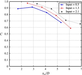
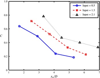
at the downstream position, shown in figure 7 for PSE. Correlations of up to 0.8 are observed for small axial separations between input and output. The correlation decreases as the output station is moved downstream away from the potential core of the jet, a consequence of the limitations of the linear model.
Peak correlation between PSE predicted signal and the measured data.

Another interesting characteristic is the fact that the correlation increases when the input is moved from
 $0.5D$
to
 $2.1D$
. This is consistent with the observations of Cavalieri et al. (Reference Cavalieri, Rodríguez, Jordan, Colonius and Gervais2013) that PSE predictions differ from experimental data in the first axial region, up to
 $x/D=2$
, due to a transition of the fluctuations from the boundary layer exiting nozzle to the Kelvin–Helmholtz mode.
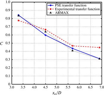
The trend is similar for the empirical transfer function and ARMAX estimations, as shown in figure 8 with a comparison of the peak correlation values, for the three methods for input position
 $x/D=2.1$
.
Peak correlation between the predicted signal with the different methods and the measured data considering the input at
 $x_{o}/D=2.1$
.

The results of this section show that real-time, low cost modelling of wavepackets in high Reynolds number turbulent jets is possible and constitutes a promising candidate for use in closed-loop control. The PSE model presents a number of additional advantages compared to the other two: (i) it does not require unsteady experimental data (a Reynolds-averaged Navier–Stokes computation could suffice to obtain the mean flow upon which linearisation is performed); (ii) large numbers of input–output pairs can be considered, which allows for the construction of a multiple-output model; (iii) different flow variables can easily be calculated. Points (ii) and (iii) will be presented further in § 5.
So far, the predictions considered only the axisymmetric mode,
 $m=0$
, which is the most efficient in what concerns acoustic radiations in the shallow angles to the jet. The PSE transfer function prediction was also tested at the azimuthal number
 $m=1$
, presenting a similar performance; these results are briefly shown in the Appendix. Combinations of frequency and azimuthal wavenumber where wavepacket models are known to be effective show compelling correlations between prediction and measurements in the time domain. The determination of the limits of the PSE prediction, in terms of frequency and azimuthal number, is a topic of current study by this group and preliminary results may be found in Cavalieri et al. (Reference Cavalieri, Sasaki, Schmidt, Colonius, Jordan and Bres2016).
4.2 Proper orthogonal decomposition filtered results
All of the analyses so far considered the axisymmetric mode of the near-field pressure without any filtering. It has previously been shown however that filtering using proper orthogonal decomposition (POD) can constitute an efficient means by which to remove fluctuations not associated with the linear waves (Suzuki & Colonius Reference Suzuki and Colonius2006; Gudmundsson & Colonius Reference Gudmundsson and Colonius2011; Breakey et al. Reference Breakey, Jordan, Cavalieri, Léon, Zhang, Lehnasch, Colonius and Rodriguez2013). The performance of the three models is now reconsidered using data filtered in this way. We follow the POD filtering strategy proposed by Breakey et al. (Reference Breakey, Jordan, Cavalieri, Léon, Zhang, Lehnasch, Colonius and Rodriguez2013), Sinha et al. (Reference Sinha, Rodríguez, Brès and Colonius2014).
The pressure signals from the finer-resolution campaign may be decomposed into frequency components (equation (4.2)),
 $$\begin{eqnarray}P_{m,\unicode[STIX]{x1D714}}(x)=P(x,m,\unicode[STIX]{x1D714})=\int \tilde{p}_{m}(x,t)\text{e}^{\text{i}\unicode[STIX]{x1D714}t}\,\text{d}t.\end{eqnarray}$$
Following Breakey et al. (Reference Breakey, Jordan, Cavalieri, Léon, Zhang, Lehnasch, Colonius and Rodriguez2013), for each frequency, the two-point cross-spectral matrix is computed as,
 $$\begin{eqnarray}\unicode[STIX]{x1D619}_{m,\unicode[STIX]{x1D714}}(x,x^{\prime })=\langle P_{m,\unicode[STIX]{x1D714}}(x)P_{m,\unicode[STIX]{x1D714}}^{\ast }(x^{\prime })\rangle ,\end{eqnarray}$$
where
 $\langle -\rangle$
is an ensemble average and the symbol
 $\ast$
indicates the complex conjugate, so that the POD problem reduces to the Fredholm integral equation,
 $$\begin{eqnarray}\int \unicode[STIX]{x1D619}_{m,\unicode[STIX]{x1D714}}(x,x^{\prime },r,r^{\prime })\unicode[STIX]{x1D6F7}_{m,\unicode[STIX]{x1D714}}(x^{\prime },r^{\prime })r^{\prime }\,\text{d}x^{\prime }=\unicode[STIX]{x1D706}_{m,\unicode[STIX]{x1D714}}\unicode[STIX]{x1D6F7}_{m,\unicode[STIX]{x1D714}}(x,r),\end{eqnarray}$$
with
 $r=(x-X_{0})\tan \unicode[STIX]{x1D6FC}$
, where
 $X_{0}$
is the virtual origin of the antenna array,
 $\unicode[STIX]{x1D6FC}$
the cone half-angle
 $\unicode[STIX]{x1D706}_{m,\unicode[STIX]{x1D714}}^{(i)}$
and
 $\unicode[STIX]{x1D6F7}_{m,\unicode[STIX]{x1D714}}^{(i)}(x)$
are the eigenvalues and eigenvectors of the matrix
 $\unicode[STIX]{x1D619}_{m,\unicode[STIX]{x1D714}}(x,x^{\prime })$
. The kernel
 $r^{\prime }\unicode[STIX]{x1D619}_{m,\unicode[STIX]{x1D714}}(x,x^{\prime },r,r^{\prime })$
is made Hermitian by multiplying equation (4.4) by
 $\sqrt{r}$
(further details are found on Breakey et al.
Reference Breakey, Jordan, Cavalieri, Léon, Zhang, Lehnasch, Colonius and Rodriguez2013), so that the eigenvalues are real and greater than or equal to zero. The eigenvalues are then ordered such that
 $\unicode[STIX]{x1D706}_{m,\unicode[STIX]{x1D714}^{(1)}}>\unicode[STIX]{x1D706}_{m,\unicode[STIX]{x1D714}^{(2)}}>\unicode[STIX]{x1D706}_{m,\unicode[STIX]{x1D714}^{(3)}}>\cdots >0$
while the eigenvectors
 $\unicode[STIX]{x1D731}_{m,\unicode[STIX]{x1D714}}^{(i)}$
are normalised such that
 $\Vert \unicode[STIX]{x1D6F7}_{m,\unicode[STIX]{x1D714}}^{(i)}\Vert =1$
. In the discrete case, the matrix has dimensions
 $N\times N$
where
 $N$
is the number of axial observation locations.
By construction, each set,
 $[\unicode[STIX]{x1D6F7}_{m,\unicode[STIX]{x1D714}}^{(i)},i=1\cdots N]$
, forms an orthonormal basis. Complex-valued coefficients of each POD mode
 $b_{m,\unicode[STIX]{x1D714}}^{(i)}$
, can be determined by projecting the Fourier transformed time signals of the azimuthal coefficients,
 $P_{m,\unicode[STIX]{x1D714}}(x)$
, onto this basis,
 $$\begin{eqnarray}b_{m,\unicode[STIX]{x1D714}}^{(i)}=(P_{m,\unicode[STIX]{x1D714}}(x),\unicode[STIX]{x1D6F7}_{m,\unicode[STIX]{x1D714}}^{(i)}(x))=\int P_{m,\unicode[STIX]{x1D714}}(x)\unicode[STIX]{x1D6F7}_{m,\unicode[STIX]{x1D714}}^{\ast (i)}(x)\,\text{d}x.\end{eqnarray}$$
Each realisation,
 $P_{m,\unicode[STIX]{x1D714}}(x)$
, is expanded in terms of
 $N_{rec}$
orthogonal basis functions with the coefficients
 $b_{m,\unicode[STIX]{x1D714}}^{(i)}$
:
 $$\begin{eqnarray}P_{m,\unicode[STIX]{x1D714}}(x)\sim \mathop{\sum }_{i=1}^{N_{rec}}b_{m,\unicode[STIX]{x1D714}}^{(i)}(x),\end{eqnarray}$$
and a low-order estimate of the time-domain signal for an azimuthal mode
 $m$
can then be formed by an inverse Fourier transform. In what follows, this low-order estimate considers the first POD mode only (i.e.
 $N_{rec}=1$
), as in prior studies. Further details may be found in Breakey et al. (Reference Breakey, Jordan, Cavalieri, Léon, Zhang, Lehnasch, Colonius and Rodriguez2013).
Figure 9 presents the comparison of the PSE time-domain transfer function convolved with POD filtered experimental data and its comparison to the actual POD filtered measured data, for the same input–output pairs of figure 6. The peak correlation values are shown in figure 10. Although not presented, a similar trend is observed when ARMAX or the experimental transfer function are used to perform the estimation.
Comparison between measured non-dimensional pressure fluctuations POD filtered (in blue) and PSE transfer function prediction (in red) for
 $x_{i}/D=0.5$
,
 $1.3$
and
 $2.1$
, on the first, second and third lines, respectively.

The performance of the three methods is considerably improved when the POD filtering is applied to the original input–output near-field data. This supports the idea that the POD filtering retains the salient correlated wavepacket dynamics, which is well predicted by the transfer function. A deterioration nonetheless persists as the output position is moved downstream, away from the potential core of the jet. However, the correlation between prediction and POD-filtered pressure is at least 0.6 for the cases studied here.
5 Single-input–multiple-output systems using PSE
There are three main advantages of the PSE transfer function. The first is that it allows for easy construction of a multiple output system. The second is that it does not require unsteady data at the output position, neither to build the transfer function nor to perform the prediction. The third is that the computational cost involved in the prediction is low, as once the reduced-order model has been built, only a convolution (which is inexpensive in computational terms) is required to the obtain the fluctuations at the output positions.
The transfer function (equation (3.8)) can therefore be obtained between any combination of the dependent variables and for any number of input–output pairs. This means that, using measurements of a single quantity (pressure for instance) at a single location in the flow, the entire flow field (all dependent variables) can be estimated. As discussed in § 3 only fluctuations associated with linear wavepackets can be obtained.
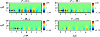
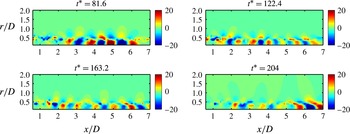
Figures 11 and 12 provide illustrations of this. Full-field pressure and velocity fluctuations are estimated using the experimental pressure data measured at
 $x/D=0.5$
(as given in figure 5). As the time series convolved with the PSE transfer function was positioned at
 $(x/D,r/D)=(0.5,0.57)$
, the fluctuation is seen to propagate from that position.
Peak correlation values between the PSE transfer function prediction and measured data, considering POD filtered values.

PSE transfer function pressure field prediction for several time slices obtained from measurements along the
 $x/D=0.5$
ring.

PSE transfer function axial velocity field prediction for several time slices, obtained from measurements along the
 $x/D=0.5$
ring.

6 Conclusions
Three strategies were used to construct time-domain, reduced-order models for axisymmetric wavepackets in a high Reynolds, turbulent jet. All three are based on the construction of a transfer function between axially and radially separated points in the flow. Using unsteady pressure measurements in the near-nozzle region, the models were used to estimate the downstream evolution of the hydrodynamic pressure field, and evaluated by comparing the estimates with measurements.
The three techniques that were evaluated differed considerably in terms of the necessary level of empiricism for their construction; while the PSE-based transfer functions, founded on the linearised governing equations, required only the mean field, ARMAX and the empirical transfer function to be fed with the full nonlinear unsteady data, in order to craft the model. In spite of such a fact, their behaviours were comparable, with the most compelling comparisons over the axial range spanned by the potential core, and the highest correlation values in regions where the wavepacket models agree best with experimental data, deteriorating further downstream.
Such deterioration indicates that closed-loop control based on PSE transfer functions may only be possible in the upstream portion of the jet, where the Kelvin–Helmholtz wavepackets experience exponential growth and dominate the dynamics. Acting in this region, however, leads to significant alterations of the far acoustic field, as shown in the works of Koenig et al. (Reference Koenig, Sasaki, Cavalieri, Jordan and Gervais2016), Le Rallic, Jordan & Gervais (Reference Le Rallic, Jordan and Gervais2016), which use an open-loop actuator in the centreline of the jet, within its potential core. Although we expect differences between open- and closed-loop control applications, the open-loop results in the cited works highlight that modifications of the upstream jet dynamics may lead to significant reductions of radiated sound. Hence, the techniques applied in this work appear promising for noise reduction closed-loop control in jets.
Furthermore, the comparable performance of a first-principles model in comparison to identification methods provides further evidence of the relevance of the wavepacket structure, not only as a statistical quantity, but as an entity allowing for a time-domain description of the flow, which is what we hypothesise the two more empirically dependent strategies are identifying. This is further evidenced by the fact that all three methods seem to miss the same portions of the signal, indicating that similar trends are being captured by them.
The most interesting and versatile of the three approaches appears to be that based on linear PSE: it presents a low computational cost both for the construction of the model and the realisation of the real-time prediction. It also allows obtaining a SIMO model to predict the behaviour of the flow variables along the field without the need for unsteady data of the solution. Such characteristics make it an attractive option for use in real-time estimation and control of wavepackets, which are known to play an important role for the radiated sound.
Comparison between the real parts of measured non-dimensional pressure fluctuations (solid line) and PSE transfer function prediction (dashed line) for
 $m=1$
and
 $x/D=0.5$
, 1.3 and 2.1 as the considered input, in the first, second and third lines, respectively.

Peak correlation between PSE predicted signal and the measured data, for the first helical mode.

There is currently an effort by this group to control wavepackets of a high Reynolds turbulent jet, using the PSE and empirical transfer functions as the basis of reduced-order time-domain models. The application of such methods for closed-loop control has already been explored for a simpler system, a two-dimensional shear layer, for which a nonlinear simulation was available, allowing for testing of the derived control laws. Preliminary results (Sasaki et al. Reference Sasaki, Tissot, Cavalieri, Silvestre, Jordan and Biau2016) show that the correlations between prediction and the nonlinear direct numerical simulation are sufficient to derive an effective feed forward control strategy for attenuation of the velocity fluctuations, delaying vortex roll up and pairing, the main sound generation mechanism in these flows (Colonius, Lele & Moin Reference Colonius, Lele and Moin1997; Wei & Freund Reference Wei and Freund2006). In this study, closed-loop control led to reductions of turbulent kinetic energy of up to 50 %.
Aside from the utility of the approach for closed-loop control of jets, the results of the PSE transfer function show that linear wavepacket models can not only predict statistical quantities, such as power spectral densities, but also the instantaneous fluctuations of flow variables of turbulent jets. This is a further demonstration of the pertinence of wavepacket modes for large-scale structures in turbulent jets.
Acknowledgements
The authors thank D. Breakey for his careful measurements of near-field pressure, which made possible the developments of the techniques described in this work. The work described was partially supported by the French National Research Agency (ANR) via COOL-JAZZ, by the European-Union program JERONIMO, by the Science Without Borders program (project no. A073/2013) and by CNPq (grant 444796/2014-2). A.V.G.C. acknowledges support via a CNPq research scholarship. K.S. acknowledges the Specialization Program in Engineering, a program by Embraer via Casemiro Montenegro Foundation.
Appendix
The axisymmetric and first helical modes are known to dominate the acoustic radiation at shallow polar angles. In this appendix we extend the PSE transfer function prediction and its comparison against experimental data, for the first helical mode (
 $m=1$
). The procedure to calculate the transfer function and convolution with the input is the same as that outlined in § 3.1.2.
Figure 13 presents the time-domain comparison between the PSE transfer function prediction and actual measurements. Similar trends as those corresponding to the axisymmetric case are seen here; a good agreement when input and output positions are close and within the potential core of the jet, and a deterioration as they are moved apart, of the amplitude more so than that of the phase and characteristic frequencies. Figure 14 presents the peak correlations between prediction and measurement, confirming this idea.
The similar performances observed for the PSE transfer function prediction between
 $m=0$
and
 $m=1$
make it probable that the effectiveness of the derived time-domain models will remain at higher azimuthal numbers, for combinations of frequency, azimuthal wavenumber and axial position where the frequency-domain characteristics are well captured by the PSE. The validity of the PSE prediction, in the frequency domain has been recently extended to Strouhal numbers as high as
 $St=4.0$
, in another study by this group (Cavalieri et al.
Reference Cavalieri, Sasaki, Schmidt, Colonius, Jordan and Bres2016).