

Many handbooks and courses in research methods and statistics seem to imply that groups have to be compared in order to conduct proper scientific research in the health sciences (see e.g., Jacobson, Reference Jacobson2017; Moore, McCabe, & Craig, Reference Moore, McCabe and Craig2017; Peat, Reference Peat2002). In those handbooks and courses, treatment effects are inferred by applying treatments to one or more experimental groups and by comparing their results to one or more control groups. The mantra is: ‘Take a random sample of patients and randomly assign these patients to treatment and control’. In medicine, this mantra is consolidated in the randomised controlled trial being the gold standard (Kaptchuk, Reference Kaptchuk2001; Sackett, Rosenberg, Gray, Haynes, & Richardson, 1996; Turner et al., Reference Turner, Shamseer, Altman, Weeks, Peters, Kober and Moher2012).
The practical disadvantages and ethical concerns of this group-comparison approach are well documented (Carey & Stiles, Reference Carey and Stiles2016), but more importantly, questions regarding the epistemological status of the results, and therefore also the clinical relevance, can be raised (Molenaar, Reference Molenaar2004; Onghena, Reference Onghena and Berger2007; Onghena & Edgington, Reference Onghena and Edgington2005). Intra-patient variability differs fundamentally from inter-patient variability, and consequently there is a fundamental difference between the meaning of a treatment effect in group-comparison studies and the meaning of a treatment effect for an individual patient (Molenaar & Campbell, Reference Molenaar and Campbell2009; Velicer & Molenaar, Reference Velicer, Molenaar, Schinka and Velicer2013). The reckless generalisation of group-comparison treatment effects to individual-patient treatment effects can be considered as a prime example of the well-known ecological fallacy (Harrington & Velicer, Reference Harrington and Velicer2015; Onghena, Reference Onghena and Berger2016). Group-comparison treatment effects are not necessarily representative of individual-patient treatment effects; it might well be that the average pattern of group differences does not apply to any single patient involved in the study (Barlow, Nock, & Hersen, Reference Barlow, Nock and Hersen2009; Gast & Ledford, Reference Gast and Ledford2014; Kazdin, Reference Kazdin2011). As Sidman (1952) already observed: ‘It appears, then, that when different groups of subjects are used to obtain the points determining a functional relation, the mean curve does not provide the information necessary to make statements concerning the function for the individual’ (p. 268).
The alternative approach that we discuss in this paper turns the group-comparison model upside down. Instead of focusing on group-comparison treatment effects, leaving us with the impossibility to generalise to individual-patient treatment effects, we start by testing the treatment effect in an individual patient and by investigating the replicability in other patients afterwards. As Shapiro (Reference Shapiro1966) put it:
It seems, therefore, that when one investigates change one cannot combine data from a number of individuals unless he knows that the differences among the curves obtained from the individuals are due to experimental error. The first step in the investigation of processes must logically consist of investigation in a number of individual cases. (p. 5)
This approach has a closer resemblance to clinical practice than the group-comparison approach: Patients enter a hospital or clinical trial one by one, and clinical care is aimed at individual patients. This closer resemblance of the individualised approach to actual clinical practice may also foster the generalisation of the results to this practical setting (i.e., increase the ecological validity of the study results) (Onghena & Edgington, Reference Onghena and Edgington2005; Tate, Aird, & Taylor, Reference Tate, Aird and Taylor2013).
Statistical models for the group-comparison approach and for the analysis of RCTs are well-established (see e.g., Jacobson, Reference Jacobson2017; Peat, Reference Peat2002). In the present paper, we want to propose a generic model for the analysis of data from replicated experiments with individual patients or, more generally, from replicated ‘single-case experiments’ (SCEs) as they are called in the methodological literature. We will try to reach this aim by
-
• Examining the specific features of SCEs that preclude the mere adoption of the common statistical techniques known from the group-comparison approach;
-
• Looking for a statistical model that takes these features into account;
-
• Proposing the use of meta-analytical procedures for the aggregation of replicated SCEs.
We will demonstrate our proposal with real-life data and apply some alternative and complementary approaches on the same data.
Definition of Single-Case Experiment
If we want a generic model for the analysis and meta-analysis of SCEs, then it is crucial to be crystal clear about the kind of data we are dealing with. We need to know exactly what the experimental units are, which units are considered in the statistical analysis, and which units are considered in the meta-analysis. In this first section, we reflect on the SCE definition and comment on the essential ingredients and their implications.
SCEs are defined as ‘experiments in which one entity is observed repeatedly during a certain period of time, under different levels (‘treatments’) of at least one independent variable’ (Onghena, Reference Onghena, Everitt and Howell2005, p. 1850). There are two essential features in this definition. First, only one entity is involved (it is a single case), and second, there is a manipulation of the independent variable(s) (it is an experiment). Two other features are consequences of this set-up: the entity is exposed to all levels of the independent variable (like in a within-subject design) and there are repeated observations or measurements (like in a longitudinal or time series design).
For the purpose of this paper it is important to reflect on the main terms and implications of this definition. We summarise our reflection in seven comments:
-
1. The definition refers to the generic term ‘entity’ to emphasise that any experimental unit at any level of aggregation may be involved. In the health sciences, the entity usually is a patient but the entity can also be a group of patients in a hospital ward, a part of a patient (e.g., a brain region), or a more abstract unit, such as a rehabilitation centre as an organisation (Barlow, Nock, & Hersen, Reference Barlow, Nock and Hersen2009; Kazdin, Reference Kazdin2011; Onghena, Reference Onghena, Everitt and Howell2005).
-
2. The definition and the following discussion of statistical techniques are restricted to ‘experiments’. By referring to one or more manipulated variables, SCEs are distinct from qualitative and descriptive case studies and from observational time series studies (Onghena & Edgington, Reference Onghena and Edgington2005; Onghena & Struyve, Reference Onghena, Struyve, Balakrishnan, Brandimarte, Everitt, Molenberghs, Piegorsch and Ruggeri2015).
-
3. Notice that the ‘observed repeatedly’ in the definition does not need to refer to measurements of quantitative attributes. Also qualitative and naturalistic observations are possible without losing the experimental nature of the SCE. However, if the data have to be analysed statistically, all observations have to be quantitatively coded in one or more outcome variables. In the remainder of this article, we assume that measurement of a quantitative attribute is at the basis of at least one outcome variable. This is the most characteristic way that SCEs are presented, and is most feasible with the rising popularity of health care wearables and ecological momentary assessment (McDonald & Davidson, Reference McDonald and Davidson2016; Piwek, Ellis, Andrews, & Joinson, Reference Piwek, Ellis, Andrews and Joinson2016).
-
4. The internal and statistical-conclusion validity of an SCE can be strengthened by including randomisation in the design (Dugard, File, & Todman, Reference Dugard, File and Todman2011; Edgington, Reference Edgington1996; Heyvaert, Wendt, Van den Noortgate, & Onghena, Reference Heyvaert, Wendt, Van den Noortgate and Onghena2015; Kratochwill & Levin, Reference Kratochwill and Levin2010), but randomisation is not a necessary feature in the SCE definition. Randomisation can be performed with respect to the treatment order or the moments of phase change or a combination of both (Levin, Ferron, & Gafurov, Reference Levin, Ferron and Gafurov2014; Onghena, Vlaeyen, & de Jong, Reference Onghena, Vlaeyen, de Jong and Sawilowsky2007).
-
5. External validity and generalisability to other patients is not always the first aim of an SCE (Barlow et al., Reference Barlow, Nock and Hersen2009; Gast & Ledford, Reference Gast and Ledford2014; Kazdin, Reference Kazdin2011). In a purely idiographic approach, the clinician might just be interested to understand and help the single patient under investigation, and may use a customised treatment and a customised symptoms checklist. However if generalisability is an aim, it can be accomplished by replications using identical (or similar) treatments and outcome measures. Replicated demonstrations of a similar treatment effect in consecutive patients provide evidence for an identical underlying process or a general law.
-
6. Many experimental design schedules are possible for SCEs. A useful classification has been proposed by Shamseer et al. (Reference Shamseer, Sampson, Bukutu, Schmid, Nikles and Tate2015), Tate et al. (Reference Tate, Perdices, Rosenkoetter, McDonald, Togher, Shadish and Vohra2016a, Reference Tate, Perdices, Rosenkoetter, Shadish, Vohra, Barlow and Wilson2016b), and Vohra et al. (Reference Vohra, Shamseer, Sampson, Bukutu, Schmid and Tate2015). They distinguish:
-
• Withdrawal or reversal designs (such as ABA, ABAB, ABACAD with each letter representing a phase of repeated measurements for the same level of the manipulated variable),
-
• Alternating treatments designs
-
• Multiple baseline designs, and
-
• Changing criterion designs.
A two-phase AB design is not included in this classification, although the use of this design in an experimental context would match the definition of an SCE. Our proposal would be to consider studies using an AB design as SCEs, but to acknowledge that this design is the poorest design in terms of methodological quality. Two-phase AB designs suffer from the fact that there is only one demonstration of the treatment effect and that effect might be due to an external event accidentally coinciding with the moment of phase change (Kratochwill et al., Reference Kratochwill, Hitchcock, Horner, Levin, Odom, Rindskopf and Shadish2010, Reference Kratochwill, Hitchcock, Horner, Levin, Odom, Rindskopf and Shadish2013; Tate et al., Reference Tate, Aird and Taylor2013). This should not mean that applied studies using an AB design are, by definition, poorest in terms of methodological quality. SCEs using an AB design may involve methodological add-ons to be able to provide solid evidence, such as a randomly timed intervention, a large number of reliable observations, and replications across patients to obtain sufficient statistical power (Barlow et al., Reference Barlow, Nock and Hersen2009; Heyvaert et al., Reference Heyvaert, Hannes and Onghena2017; Heyvaert, Wendt, Van den Noortgate, & Onghena, Reference Heyvaert, Wendt, Van den Noortgate and Onghena2015).
-
-
7. In the medical literature, the term ‘N-of-1 trial’ has been adopted to refer to a prospectively planned, multiple crossover trial in a single patient to determine the effect of an intervention (Guyatt, Jaeschke, & McGinn, Reference Guyatt, Jaeschke, McGinn, Guyatt, Rennie, Meade and Cook2002; Schork, Reference Schork2015; Shamseer et al., Reference Shamseer, Sampson, Bukutu, Schmid, Nikles and Tate2015; Vohra et al., Reference Vohra, Shamseer, Sampson, Bukutu, Schmid and Tate2015). N-of-1 trials are ‘biomedical’ SCEs, usually using a withdrawal or reversal design. Furthermore, N-of-1 trials often evaluate pharmacological treatments and include placebo control, randomisation, and blinding (Onghena, Reference Onghena and Berger2007, Reference Onghena and Berger2016). Consequently N-of-1 trials can be considered a subset of SCEs (Tate et al., Reference Tate, Perdices, Rosenkoetter, McDonald, Togher, Shadish and Vohra2016a, Reference Tate, Perdices, Rosenkoetter, Shadish, Vohra, Barlow and Wilson2016b).
An Example
An example of a replicated SCE with two patients was published in this journal by Douglas, Knox, De Maio, and Bridge (Reference Douglas, Knox, De Maio and Bridge2015). They used an AB design with follow-up to evaluate the effectiveness of a new treatment, Communication-specific Coping Intervention (CommCope-I), which targets coping in the context of communication breakdown after traumatic brain injury. The study was carried out with two patients: Samantha,Footnote 1 a 30-year-old woman, and Thomas, a 34-year-old man, who both had sustained severe traumatic brain injury several years before, and still experienced substantial communication problems. The primary outcome variable in this study was the Discourse Coping Scale – Clinician Rating, which uses a 10-cm visual analogue scale to measure the appropriate use of communication-specific coping strategies.
The raw data of the first A phase and the B phase are shown in Tables 1 and 2 for Samantha and Thomas respectively. As can be seen in the tables all scores in the B phase are larger than the scores in the A phase and the authors conclude that: ‘This study provides sound phase-1 evidence for the effectiveness of CommCope-I’. (p. 190).
Weekly Scores on the Discourse Coping Scale – Clinician Rating for Samantha During a 9-Week SCE with a 3-Week Baseline (A phase) and a 6-Week Communication-Specific Coping Intervention (B phase)

Note. There was one missing week and data point in the A phase.
Weekly Scores on the Discourse Coping Scale – Clinician Rating for Thomas During a 9-Week SCE with a 4-Week Baseline (A phase) and a 6-Week Communication-Specific Coping Intervention (B phase)

In the remainder of this article we will use the data in Tables 1 and 2 for a simple numerical demonstration of the statistical analysis and meta-analysis of SCE data. In most applications, the data are more numerous, complicated, diverse or fragmented and we will reflect on a few of these complicating issues (and their solutions) in the Discussion section. Furthermore, Table 1 and Table 2 contain two simplifications compared to the original data in Douglas et al. (Reference Douglas, Knox, De Maio and Bridge2015):
-
1. We ignored the missing data point in the A phase of Samantha because dealing with missing data is a separate and complicated issue that would distract from the main ideas in the demonstration.
-
2. Douglas et al. (Reference Douglas, Knox, De Maio and Bridge2015) referred to their design as ‘an ABA design’ (p. 194), but as the authors acknowledged: ‘The withdrawal design is somewhat limited in the case of skill-based interventions like CommCope-I which are designed to facilitate lasting change in behaviour and are thus not strictly amenable to evaluation using return to baseline single-case designs’. (p. 199) If the data in the follow-up phase were modelled as ‘a return to baseline phase’ then the results would be opposite to what is expected. Consequently, for both Samantha and Thomas, we did not include the follow-up data to avoid this interpretational pitfall.
We will also return to the implications of these simplifications and refer to some statistical options to deal with missing data and withdrawal designs in the Discussion section. The Appendix presents R code for all computations that are used in this manuscript.
A Simple Statistical Model for the AB Design: Model 1
Taking into account the essential and implied features of the SCE definition, a simple statistical model for data from a single patient considers the patient as the population and the repeated measurements as a random sample (i.e., realisations of a random outcome variable). In an AB design, the manipulated variable takes two values: one value for the baseline phase and one value for the treatment phase.
Given these features, some authors have been analysing data from SCEs using the following simple statistical model (Gentile, Roden, & Klein, Reference Gentile, Roden and Klein1972; Shine & Bower, Reference Shine and Bower1971):
 $$\begin{equation}
{\rm{Scor}}{{\rm{e}}_t} = {\beta _0} + {\beta _1}{\left( {{\rm{Treat}}} \right)_t} + {\varepsilon _t}
\end{equation}$$
with
-
Score t referring to the value of the outcome variable at time t; the outcome variable Score indicates the repeated measurements, with the index t going from 1 to N (for N repeated measurements available from the SCE),
-
(Treat) t , referring to the manipulated variable, taking a value of 0 for each measurement occasion in the baseline phase and a value of 1 for each measurement occasion in the treatment phase,
-
β0 referring to the baseline mean (i.e., the value of Score t when (Treat) t and ε t equal 0),
-
β1 referring to the difference between the treatment mean and the baseline mean (i.e., the treatment effect),
-
ε t referring to the residual at time t, which is the deviation of Score t from the average value of the outcome variable in the corresponding phase, ε t = Score t − [β0 + β1(Treat) t ].
The values for Score t are observed by conducting the study and the values of (Treat) t are determined by the chosen design; the values for β0 and β1 have to be derived following a particular optimisation criterion. The classical optimisation criterion is the minimisation of the squared residuals ε2 t , resulting in a so-called ‘Ordinary Least Squares’ (OLS) regression (or a common Analysis of Variance, using slightly different notation).
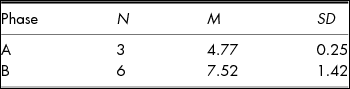
For the data of Samantha in Table 1, we have N equal to 9, and the means and standard deviations as shown in Table 3.
Summary Statistics for the Samantha Data in Table 1

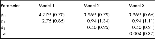
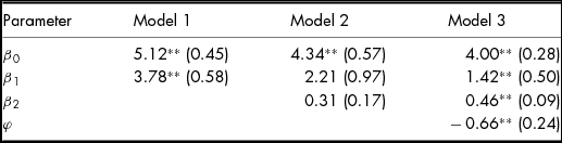
For Model 1 we obtain β0 = 4.77 and β1 = 2.75 (see the first two columns of Table 4), so there is an average addition of 2.75 points for the scores in the B phase as compared to the A phase, which can also be verified in Table 3 (4.77 + 2.75 = 7.52). Notice that no distributional assumptions are needed for the derivation of the OLS estimates.
Parameter Estimates (and Standard Errors) of the Models Specified in Equations 1–3 for the Samantha Data in Table 1

Note. *p < .05. **p < .01.
A distributional model is usually invoked if questions like: ‘Is this value of β1 = 2.75 statistically significantly different from zero?’ or ‘What is the 95% confidence interval for this treatment effect estimate?’ need an answer. The most common model arises if the ε t values are assumed to be independent and identically distributed Gaussian deviates with a mean of 0 and an unknown variance σ2 ε (ε t ~ N(0, σ2 ε)). Under this assumption, the treatment effect for the Samantha data is considered statistically significant, β1 = 2.75, t(7) = 3.22, p = .0146, with [0.73; 4.77] being the 95% confidence interval.Footnote 2 Notice that the same t- and p-values would be obtained if a classical two-sample Student t test was performed or an equivalent F (= t²) and identical p-value for an Analysis of Variance with two independent groups.Footnote 3 Notice also that the statistical test for the β0 parameter is usually not relevant because it is testing a hypothesis that is irrelevant for most applications, namely the null hypothesis that the baseline mean is zero, H0: β0 = 0.
The assumption with regard to the residuals can be relaxed by only assuming that the residuals are exchangeable, so without specifying any population distributional shape. In that case an exact regression permutation test can be performed (Ottoboni, Lewis, & Salmaso, Reference Ottoboni, Lewis and Salmaso2017; Pesarin & Salmaso, Reference Pesarin and Salmaso2010; Wheeler & Torchiano, Reference Wheeler and Torchiano2016), with a result that is very similar to the Gaussian theory test, perm t(7) = 4.037, p = .0238. This value can easily be verified because there is no overlap between the scores in the two phases. In that case, the observed test statistic provides the most extreme value and the exact one-sided permutation test p-value can be obtained by inverting the binomial coefficient
 ${( \scriptsize{\begin{array}{@{}*{1}{c}@{}} N\\ n \end{array} )^{ - 1}}}$
. The exact two-sided permutation test p-value can be obtained by doubling this value. For the Samantha data 2/
 $(\scriptsize{\begin{array}{@{}*{1}{c}@{}} 9\\ 3 \end{array}} )$
= .0238. This procedure is equivalent to the procedure in a two-sample permutation test (Edgington & Onghena, Reference Edgington and Onghena2007; Fay, Reference Fay2010), so also for this test the same p-value of .0238 would be obtained.
Modelling Trend: Model 2
Equation (1) is overly simplistic because it only models a difference between the A phase average and the B phase average. By contrast, an SCE always involves a time component and usually there is an evolution in time within the phases, a so-called ‘trend’ (Shadish & Sullivan, Reference Shadish and Sullivan2011; Solomon, Reference Solomon2014). Therefore, a more appropriate statistical model for time series data includes a parameter β2 to capture this trend:
 $$\begin{equation}
\hspace*{-8pt}{\rm{Scor}}{{\rm{e}}_t} = {\beta _0} + {\beta _1}{\left( {{\rm{Treat}}} \right)_t} + {\beta _2}{\left( {{\rm{Time}}} \right)_t} + {\varepsilon _t}
\end{equation}$$
with
-
Score t and (Treat) t identical as in Equation 1,
-
(Time) t referring to the value of the time variable at time t; for the models in this manuscript the time variable takes the same values as the index t (viz, from 1 to N for Week 1 to Week N), but for more sophisticated models other values can be used,Footnote 4
-
β0 referring to the intercept, that is the expected value of the outcome variable Score when (Treat) t and (Time) t are zero,
-
β1 referring to the change in the expected value of the outcome variable Score when going from the baseline phase to the treatment phase (i.e., the additive treatment effect),
-
β2 referring to the change in the expected value of the outcome variable for each unit change in (Time) t (i.e., the trend), and
-
ε t referring to the residual at time t, which is the deviation of Score t from the best fitting equation at time t, ε t = Score t − [β0 + β1(Treat) t + β2(Time) t ].
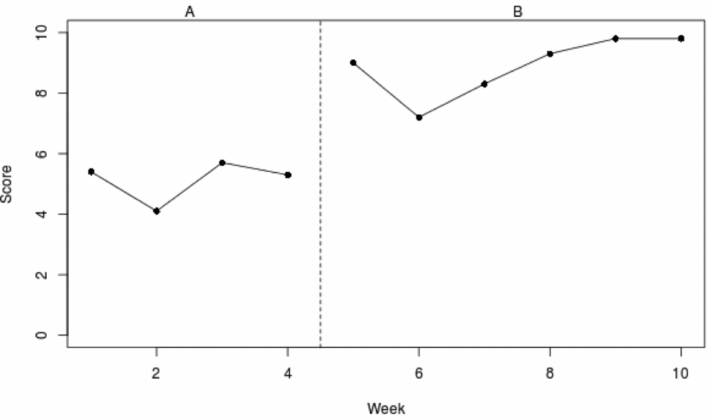
A trend can most conveniently be spotted by making a time series plot of the data. Figure 1 shows the time series plot of the Samantha data. There seems to be a steady increase in Samantha's communication from Week 1 to Week 9, but it is not clear whether that increase is statistically significant. The parameter estimates and their standard errors for this Equation (2) can be found in Table 4, in the column with ‘Model 2’ as the header.
Weekly scores on the Discourse Coping Scale – Clinician Rating for Samantha during a nine-week SCE with a three-week baseline (A phase) and a 6-week Communication-specific Coping Intervention (B phase).

If we assume that ε t ~ N(0, σ2 ε) then the additive treatment effect for the Samantha data is not considered statistically significant anymore, β1 = 0.94, t(6) = 0.70, p = .5109, with [−2.35; 4.22] being the 95% confidence interval after taking the linear trend into account. Also the trend itself is not statistically significant, β2 = 0.40, t(6) = 1.64, p = .1518, with [−0.20; 1.00] being the 95% confidence interval. The permutation test p-values are .5050 and .1550 (see Wheeler & Torchiano, Reference Wheeler and Torchiano2016, and the Appendix for the calculation of the permutation test p-values).
Notice that the β1 estimate in Equation (2), 0.94, is smaller than the β1 estimate in Equation (1), 2.75. The reason for this difference is that Equation (2) also includes a trend parameter β2 and that in the estimation all components of the equation are taken into account. The linear trend estimate in this example indicates that there is a score increase of β2 = 0.40 for each unit of change in the time variable, even if there is no additive treatment effect. For the A phase, (Treat) t = 0, this means that the expected scores are: 3.96 + (1)(0.40) = 4.36, 3.96 + (2)(0.40) = 4.76, and 3.96 + (3)(0.40) = 5.16. The average of these three numbers is 4.76, which is the A phase average (within rounding error) that can be found in Table 3. For the B phase, (Treat) t = 1, the expected scores from Equation (2) become: 3.96 + 0.94 + (4)(0.40) = 6.5, 3.96 + 0.94 + (5)(0.40) = 6.9, 3.96 + 0.94 + (6)(0.40) = 7.3, 3.96 + 0.94 + (7)(0.40) = 7.7, 3.96 + 0.94 + (8)(0.40) = 8.1, and 3.96 + 0.94 + (9)(0.40) = 8.5. The average of these six numbers is 7.5, which is the B phase average (within rounding error) that can be found in Table 3. This demonstrates that the phase averages following Equation (2) are constructed by adding three components: an intercept, a time trend, and an additive treatment effect. Consequently, the β1 estimate in Equation (2) should be interpreted differently than the β1 estimate in Equation (1). In Equation (2) the β1 estimate does not represent the raw difference between the phase averages but rather represents the score that is added in the B phase after taking the linear trend into account.
Another important difference between the results using Equation (2) as opposed to the results using Equation (1) is that the treatment effect has become statistically non-significant. This means that the treatment effect cannot be distinguished from the mere increment of the scores as a function of time. Although Figure 1 may give the impression that there is an additive treatment effect in addition to a small trend, none of these effects is large enough to be statistically significant. The observed data using this design and this (small) number of repeated measures are not convincing enough to attribute the larger average in the B phase to either an additive treatment effect or to a trend.
Modelling Serial Dependency: Model 3
A simplifying assumption that we made in the previous analyses is that the residuals are independent or exchangeable, given that all relevant parameters are included in the model. This assumption is not obvious for time series data (Harrington & Velicer, Reference Harrington and Velicer2015; Jones, Weinrot, & Vaught, Reference Jones, Weinrot and Vaught1978) and therefore Equation (2) is sometimes extended using an autoregressive parameter for the residuals:
 $$\begin{eqnarray}
&&{\rm{Scor}}{{\rm{e}}_t} = {\beta _0} + {\beta _1}{\left( {{\rm{Treat}}} \right)_t} + {\beta _2}{\left( {{\rm{Time}}} \right)_t} + {\varepsilon _t},\nonumber\\[-4pt]
&& {\rm{with}}\;{\rm{the}}\;{\rm{residuals}} \ {\varepsilon _t} = \ \varphi {\varepsilon _{t - 1}} + \ {\omega _t}{\rm{\ }}\;{\rm{and}}\nonumber\\[-4pt]
&&\quad {\omega _t} \sim N\left( {0,\sigma _\omega ^2} \right),
\end{eqnarray}$$
and with all the other parameters as defined in Equation (2).
The results are shown in Table 4, in the column with ‘Model 3’ as the header. The autoregressive parameter appears to be very small, and the results for Model 3 are essentially identical to the results for Model 2.
More Complex Statistical Models for the AB Design
It is possible to extend Equations (2) and (3) in several ways. An elaboration of these extensions is beyond the scope of the present article, but we give some references for the reader who is interested to explore these extensions.
A first possible extension is the inclusion of an interaction term (Treat) t × (Time) t to assess whether the trend changes from the baseline to the treatment phase. Issues regarding specification of the linear model, coding of the variables and interpretation are presented in a very accessible way by Huitema and McKean (Reference Huitema and McKean2000).
A second possible extension is the inclusion of non-linear terms with respect to time, such as (Time2) t to model quadratic trends. The interested reader is referred to Aiken, West, and Pitts (Reference Aiken, West, Pitts, Schinka and Velicer2003).
A third possible extension is the inclusion of additional terms to model the serial dependency. A very general methodology to accomplish this involves the use of so-called ‘Autoregressive Integrated Moving Average’ models (see Box, Jenkins, Reinsel, & Ljung, Reference Box, Jenkins, Reinsel and Ljung2016, for a modern presentation of this methodology). Those models make provision for higher-order autoregressive parameters and moving average parameters, based on repeated cycles of model identification, parameter estimation, and diagnostic checking. Furthermore, lagged predictor variables can be added to examine the relationship between the outcome variable and other manipulated or non-manipulated predictor variables with possible time delays. For example, if data about weekly mood were collected, a third predictor variable (Mood) t − 1, with the corresponding parameter β3, could be added to Equation (3) to examine the relationship between communication at week t and Mood the week before (t – 1).
For some applications, those extensions may be relevant, but essentially any modelling attempt will boil down to the three basics: modelling the treatment effect, modelling the trend and modelling the serial dependency, as demonstrated in the previous sections. Finally, notice that an important restriction in Equations (1), (2) and (3) is that a numerical outcome variable is considered. If the outcome variable is categorical, or even dichotomous, generalised models are needed (McCullagh & Nelder, Reference McCullagh and Nelder1989).
Meta-Analysis: Modelling the Nested Structure for Replicated AB Designs in Models 4, 5 and 6
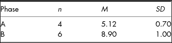
The same analyses can be performed on Thomas's data and the results can be found in Figure 2, Tables 5 and 6. For Thomas, Model 3 indicates a statistically significant treatment effect, a statistically significant linear trend, and a statistically significant negative autoregressive parameter.
Weekly scores on the Discourse Coping Scale – Clinician Rating for Thomas during a 10-week SCE with a 4-week baseline (A phase) and a 6-week Communication-specific Coping Intervention (B phase).

Summary Statistics for the Thomas Data in Table 2

Parameter Estimates (and Standard Errors) of the Models Specified in Equations 1–3 for the Thomas Data in Table 2

Note. *p < .05. **p< .01.
In this example, there are two patients, but in general, there might be J patients and for each patient j (j = 1, . . ., J) such a separate analysis can be performed. Moreover, if J is large enough and the SCEs are similar enough in design and research focus, then it might also be interesting to combine and compare the results of these multiple patients. Such a pooled analysis is called a ‘meta-analysis’ because it is an analysis at a higher level. Notice that the SCEs can be conducted simultaneously (as in multiple baseline designs across participants), at different points in time (as in replicated AB designs), at different research institutes, and the data may be extracted from different publications.
For the meta-analysis of these SCEs we will present the multilevel approach proposed by Van den Noortgate and Onghena (Reference Van den Noortgate and Onghena2003a, Reference Van den Noortgate and Onghena2003c). For illustration purposes, we will use the data from Samantha and Thomas, but judicious application of this methodology should involve samples much larger than two (see Discussion section for the factors involved in determining the appropriate number of patients). In addition, we will assume that all raw data are available; an assumption that is not unrealistic for SCEs because in the SCE literature it is good practice to have the raw data published in a table or a graph.Footnote 5 Alternatively researchers can be asked to share the raw data upon request. If the raw data are not available and the meta-analysis has to be performed on summary statistics then the effect size model proposed by Van den Noortgate and Onghena (Reference Van den Noortgate and Onghena2003b) can be used.
For the meta-analysis, we have to adjust our notation. In order to make a distinction between the models for Samantha and the models for Thomas, an additional index has to be used to specify the particular patient that is involved. So for Samantha, Equation (1) becomes Score t1 = β01 + β11(Treat) t1 + ε t1 and for Thomas Score t2 = β02 + β12(Treat) t2 + ε t2. In general, for J patients, Equation (1) becomes
 $$\begin{equation}
{\rm{Scor}}{{\rm{e}}_{tj}} = {\beta _{0j}} + {\beta _{1j}}{\left( {{\rm{Treat}}} \right)_{tj}} + {\varepsilon _{tj}}
\end{equation}$$
Furthermore, if we want to include the data of all patients in one overall meta-analysis, we have to take the nested data structure into account: there are J patients and the repeated measures are nested within the patient. So for a meta-analysis, we are considering a sample from a population of patients and in each patient a random sample of repeated measurements. The additional index j is used to indicate that all values can differ between patients, so also the parameters can vary. The variation of the parameters can be modelled with a set of regression equations at the second level:
 $$\begin{equation}
\begin{array}{@{}l@{}} {\beta _{0j}} = {\gamma _0} + {u_{0j}}\\ {\beta _{1j}} = {\gamma _1} + {u_{1j}} \end{array}
\end{equation}$$
Together Equations (4a) and (4b) constitute a simple meta-analytical model for SCEs. In this model γ0 indicates the population average score for the baseline and γ1 the difference between the population treatment average and the population baseline average. The residuals u 0j and u 1j indicate the deviations between the parameter values for each patient j and the value of the population parameter. By assuming that these residuals follow a multivariate normal distribution with zero means, variances σ2 0 and σ2 1, and covariance σ01, in symbols this is:
 $$\begin{equation}
\left( {\begin{array}{@{}*{1}{c}@{}} {\ {u_{0j}}}\\ {\ {u_{1j}}} \end{array}} \right)\ \sim\ N\left( {\begin{array}{@{}*{1}{c}@{}} 0\\ 0 \end{array}\ ,{\rm{\ }}\ \begin{array}{@{}*{1}{c}@{}} {\sigma _0^2}\\ {{\sigma _{10}}} \end{array}\begin{array}{@{}*{1}{c}@{}} {{\sigma _{01}}}\\ {\sigma _1^2} \end{array}} \right)
\end{equation}$$
we can perform statistical tests and construct confidence intervals.
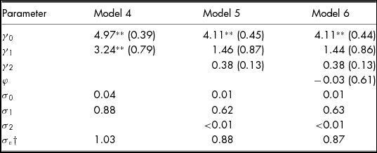
The parameter estimates and standard errors for this Model 4 can be found in Table 7 Footnote 6 . In this meta-analytical model, the average treatment effect is considered statistically significant, γ1= 3.24, t(16) = 4.09, p = .0009, with [1.56; 4.92] being the approximate 95% confidence interval. The estimated standard deviations of the random effects indicate that there is little difference between the patients with respect to their average (σ0 = 0.04), and that there are larger differences between the patients with respect to the treatment effect (σ1 = 0.88) and between the repeated measurements after taking the treatment effect into account (σε = 1.03).
Model Estimates (and Standard Errors) for the Multilevel Meta-Analysis Containing both the Samantha and Thomas Data in Tables 1 and 2

Note 1. *p < .05. **p < .01.
Note 2. Standard errors for the standard deviations of the random effects are not reported because the sampling distribution of these standard deviations is strongly asymmetrical (Pinheiro & Bates, Reference Pinheiro and Bates2000). Certainly for only two patients this standard error would be a very misleading measure of uncertainty. See Bates (Reference Bates2010) for an alternative approach.
†σω for Model 6.
Similarly, in a meta-analytical context, Equation (2) is extended to a model with three equations at the second level (one additional equation for the differences in time trend between the patients):
 $$\begin{equation}
\begin{array}{@{}l@{}} {\rm{Scor}}{{\rm{e}}_{tj}} = {\beta _{0j}} + {\beta _{1j}}{\left( {{\rm{Treat}}} \right)_{tj}} + {\beta _{2j}}{\left( {{\rm{Time}}} \right)_{tj}}\\
\quad + {\varepsilon _{tj}},\;{\rm{with}}\\ {\beta _{0j}} = {\gamma _0} + {u_{0j}},\\ {\beta _{1j}} = {\gamma _1} + {u_{1j}},\\ {\beta _{2j}} = {\gamma _2} + {u_{2j}},\\ {\rm{and}}\;\left( {\begin{array}{@{}*{1}{c}@{}} {\ {u_{0j}}}\\ {\ {u_{1j}}}\\ {\ {u_{2j}}} \end{array}} \right)\ \sim \ N\left( {\begin{array}{@{}*{1}{c}@{}} 0\\ 0\\ 0 \end{array}\ \ ,\ {\rm{\ \ }}\begin{array}{@{}*{3}{c}@{}} {\sigma _0^2}&\quad {{\sigma _{01}}}&\quad {{\sigma _{02}}}\\ {{\sigma _{10}}}&\quad {\sigma _1^2}&\quad {{\sigma _{12}}}\\ {{\sigma _{20}}}&\quad {{\sigma _{21}}}&\quad {\sigma _2^2} \end{array}} \right), \end{array}
\end{equation}$$
and Equation (3) becomes
 $$\begin{equation}
\begin{array}{@{}l@{}} {\rm{Scor}}{{\rm{e}}_{tj}} = {\beta _{0j}} + {\beta _{1j}}{\left( {{\rm{Treat}}} \right)_{tj}} + {\beta _{2j}}{\left( {{\rm{Time}}} \right)_{tj}}\\
\quad + {\varepsilon _{tj}},\;{\rm{with}}\\ {\varepsilon _t} = \ \varphi {\varepsilon _{t - 1}} + \ {\omega _t}{\rm{\ }}\quad {\rm{and}}\quad \ {\omega _t}\sim N\left( {0,\sigma _\omega ^2} \right),\\ {\beta _{0j}} = {\gamma _0} + {u_{0j}},\\ {\beta _{1j}} = {\gamma _1} + {u_{1j}},\\ {\beta _{2j}} = {\gamma _2} + {u_{2j}},\\ {\rm{and}}\;\left( {\begin{array}{@{}*{1}{c}@{}} {\ {u_{0j}}}\\ {\ {u_{1j}}}\\ {\ {u_{2j}}} \end{array}} \right)\ \sim \ N\left( {\begin{array}{@{}*{1}{c}@{}} 0\\ 0\\ 0 \end{array}\ \ ,\ {\rm{\ \ }}\begin{array}{@{}*{3}{c}@{}} {\sigma _0^2}&\quad {{\sigma _{01}}}&\quad {{\sigma _{02}}}\\ {{\sigma _{10}}}&\quad {\sigma _1^2}&\quad {{\sigma _{12}}}\\ {{\sigma _{20}}}&\quad {{\sigma _{21}}}&\quad {\sigma _2^2} \end{array}} \right). \end{array}
\end{equation}$$
The results for Model 5 show that the treatment effect is again not statistically significant anymore, γ1= 1.46, t(15) = 1.68, p =.1141, once the trend is taken into account (Table 7). The approximate 95% confidence interval for the treatment effect is [−0.40; 3.32], which obviously contains zero. The time trend is statistically significant, γ2= 0.38, t(15) = 2.82, p =.0129, with an approximate 95% confidence interval of [0.09; 0.66], which means that there is a general upward trend. The standard deviations of the random effects show the same pattern as in Model 5, with the addition that there is little difference between the patients with respect to this general time trend (σ2 < 0.01). As can be seen in Table 7, the results for Model 6 are essentially identical to the results for Model 5, due to the small (and non-significant) value for the autoregressive parameter (φ = −0.03).
According to Douglas et al. (Reference Douglas, Knox, De Maio and Bridge2015, p. 190), these SCEs provide ‘sound phase-1 evidence for the effectiveness of CommCope-I’ (p. 190), but our analysis demonstrates that with this simple design, with this statistical model, only two SCEs, and these data, it is impossible to convincingly distinguish between the treatment effect and the general time trend. Instead of calling it ‘sound phase-1 evidence’ it would be more cautious to label these results as ‘promising’. Of course, we have to acknowledge that our analysis was also tentative, based on questionable assumptions, and for demonstration purposes only. When readers would look at the complete Douglas et al. (Reference Douglas, Knox, De Maio and Bridge2015) study, including the follow-up data and more qualitative information, and they would perform an analysis based on alternative statistical models (e.g., including a (Treat) t × (Time) t interaction), then it cannot be ruled out that other conclusions are drawn.
Meta-Analysis: More Advanced Issues and Tools
The multilevel meta-analytic model can be extended in several ways. Without going into the technical details, we mention nine additions and variations, and provide the references for the interested reader:
-
1. Usually a multilevel meta-analysis is performed not only to combine the patient results, as in the example, but also to compare the patients. Formally, this comparison is carried out by adding a moderator variable at the higher-level regression equation. For example, a comparison between men and women with respect to the treatment effect in Equation (4b) is accomplished by dummy coding men and women in the data set and extending the Equation as β1j = γ10 + γ11(Sex) j + u 1j . Notice that there is no t index for this additional variable because sex only varies between patients (i.e., in the second-level equation); this variable is a characteristic of the patients, not a characteristic of the measurement occasions. Notice also that it is possible to include numerical moderator variables. For example, the patient's age can be added and also interactions between sex and age examined: β1j = γ10 + γ11(Sex) j + γ12(Age) j + γ13[(Sex) j × (Age) j ] + u 1j . If there is substantial variation in the lower-level parameter between patients (e.g., the β1’s), then the addition of moderators at the higher level will allow a better understanding of how this variation comes about (Baek et al., Reference Baek, Moeyaert, Petit-Bois, Beretvas, Van den Noortgate and Ferron2014; Van den Noortgate & Onghena, Reference Van den Noortgate and Onghena2003a; Van den Noortgate & Onghena, Reference Van den Noortgate and Onghena2008).
-
2. Multilevel meta-analysis of SCEs need not be restricted to two levels (repeated measurements within patients) as in the Samantha-Thomas example. The model can also be applied to three or more levels, for example, when a literature review involves multiple SCEs nested within each publication (three levels: repeated measurements within patients within publications) (Moeyaert, Ferron, Beretvas, & Van den Noortgate, Reference Moeyaert, Ferron, Beretvas and Van den Noortgate2014; Moeyaert, Ugille, Ferron, Beretvas, & Van den Noortgate, Reference Moeyaert, Ugille, Ferron, Beretvas and Van den Noortgate2013a, Reference Moeyaert, Ugille, Ferron, Beretvas and Van den Noortgate2013b).
-
3. Multilevel meta-analysis of SCEs need also not be restricted to one outcome variable. In many applications, there are multiple outcome variables or multiple effect size measures and the model has to be adapted accordingly. This can be accomplished in a multilevel meta-analysis by including the outcome variable as a separate level in the model (Moeyaert et al., Reference Moeyaert, Ugille, Beretvas, Ferron, Bunuan and Van den Noortgate2016; Van den Noortgate, López-López, Marín-Martínez, & Sánchez-Meca, Reference Van den Noortgate, López-López, Marín-Martínez and Sánchez-Meca2013, Reference Van den Noortgate, López-López, Marín-Martínez and Sánchez-Meca2015).
-
4. Multilevel meta-analysis of SCEs is also applicable to other designs than replicated two-phase AB designs (Moeyaert et al., Reference Moeyaert, Ugille, Ferron, Onghena, Heyvaert and Van den Noortgate2015). Moeyaert et al. (Reference Moeyaert, Ferron, Beretvas and Van den Noortgate2014) showed how design matrices can be specified for reversal designs, alternating treatments designs, and multiple-baseline designs. Brosnan et al. (Reference Brosnan, Moeyaert, Brooks Newsome, Healy, Heyvaert, Onghena and Van den Noortgate2017), for example, used such an extended multilevel model for multiple-baseline data in a study evaluating precision teaching to improve the fluency in foundational reading skills for at risk readers.
-
5. In the example, we performed the analyses at the individual patient level first, and afterwards combined the two analyses in a two-level meta-analysis. The other way around, the two-level meta-analysis also enables a more accurate estimation of the patient-level treatments effects afterwards. The advantage of these ‘empirical Bayes estimates’, using a weighted average of the estimate based on the individual patient data and an estimate based on the average of all patients’ data, is that for short time series data at the patient level it is still possible to obtain reliable estimates by ‘borrowing strength’ from the average estimate (Ferron, Farmer, & Owens, Reference Ferron, Farmer and Owens2010; Van den Noortgate & Onghena, Reference Van den Noortgate and Onghena2003a).
-
6. As mentioned before, multilevel meta-analysis of SCEs can also handle data sets with only descriptive statistics or effect sizes available. Without having access to the raw data, a multilevel meta-analysis can still be performed if sufficient information is available to estimate the sampling variance of the statistics prior to performing the meta-analysis (Ugille, Moeyaert, Beretvas, Ferron, & Van den Noortgate, Reference Ugille, Moeyaert, Beretvas, Ferron and Van den Noortgate2012; Van den Noortgate & Onghena, Reference Van den Noortgate and Onghena2003b).
-
7. Because multilevel meta-analysis of SCEs usually involves consecutive patients or consecutive publications, techniques from sequential analysis can be applied. Kuppens and Onghena (Reference Kuppens and Onghena2010) and Kuppens, Heyvaert, Van den Noortgate, and Onghena (Reference Kuppens, Heyvaert, Van den Noortgate and Onghena2011) proposed such a sequential meta-analysis of SCEs, which focuses on the question whether enough cumulative knowledge has been collected to draw convincing statistical conclusions and when data collection can be stopped. Determining the sufficiency of cumulative knowledge avoids the inefficient use of limited resources and prevents the dissemination of treatments with dubious benefits (Kuppens & Onghena, Reference Kuppens and Onghena2012).
-
8. Multilevel meta-analysis of SCEs can be completed by performing sensitivity analyses and publication bias analyses in a similar way as with standard meta-analysis (Cooper, Hedges, & Valentine, Reference Cooper, Hedges and Valentine2009). Sensitivity analyses are used to examine whether certain researcher decisions (e.g., ways of handling missing data, adding a moderator variable or not) distort the conclusions and the inferences drawn from the analysis. Publication bias analyses are used to examine whether there are indications that the results in the published literature differ systematically from the results that remain unpublished (e.g., by using a funnel plot-, calculating a fail-safe N, or performing Duval and Tweedie's trim and fill analysis). Examples of sensitivity analyses and publication bias analyses in multilevel meta-analyses of SCEs can be found in the applied studies by Heyvaert, Maes, and Onghena (Reference Heyvaert, Maes and Onghena2010), Heyvaert, Maes, Van den Noortgate, Kuppens, and Onghena (Reference Heyvaert, Maes, Van den Noortgate, Kuppens and Onghena2012), and Vanderkerken, Heyvaert, Maes, and Onghena (Reference Vanderkerken, Heyvaert, Maes and Onghena2013).
-
9. Finally, besides deriving the patient-level treatments effects using ‘empirical Bayes estimates’, it is also possible to perform a fully Bayesian analysis of multilevel data if prior distributions for the parameters can be specified. The fully Bayesian approach is promising for small data sets, offers an elegant solution for imputing missing values, and also lends itself very nicely to a sequential or cumulative meta-analysis (de Vries & Morey, Reference de Vries and Morey2013; Kravitz & Duan, Reference Kravitz, Duan, Duan, Eslick, Gabler, Kaplan, Kravitz, Larson, Pace, Schmid, Sim and Vohra2014; Moeyaert, Rindskopf, Onghena, & Van den Noortgate, Reference Moeyaert, Rindskopf, Onghena and Van den Noortgate2017).
Meta-Analysis: Alternative Methods
Applications of multilevel meta-analysis of SCEs are still scarce. Jamshidi et al. (Reference Jamshidi, Heyvaert, Declercq, Fernández Castilla, Ferron, Moeyaert and Van den Noortgate2017) reviewed 178 SCE meta-analyses and found only 22 studies (12%) that applied a multilevel analysis. This may be partly due to the fact that single-case researchers are reluctant to use advanced statistical techniques on their data. Most single-case researchers prefer visual techniques and calculate simple non-overlap measures to quantify the treatment effects in a separate SCE (Manolov & Moeyaert, Reference Manolov and Moeyaert2017a, Reference Manolov and Moeyaert2017b; Manolov this issue). For the analysis of multiple SCEs this preference translates into the use of simple methods to aggregate studies. Most SCE meta-analyses report a simple average or a range of effect sizes (Jamshidi et al., Reference Jamshidi, Heyvaert, Declercq, Fernández Castilla, Ferron, Moeyaert and Van den Noortgate2017).
In the original analysis of the Samantha-Thomas example, Douglas et al. (Reference Douglas, Knox, De Maio and Bridge2015) also based their ‘sound phase-1 evidence’ on the calculation of a non-overlap measure for each patient (with a maximum score of 100% non-overlap for each patient). They used a measure corrected for baseline trend (Manolov & Solanas, Reference Manolov and Solanas2009), but without impact for their data (because there was no noticeable baseline trend). Although the complementary use of visual techniques and the calculation of non-overlap remain strongly recommended (Lane & Gast, Reference Lane and Gast2014; Lane & Ledford this issue; Manolov this issue), the sole use of these techniques may lead to unreliable or unreplicable conclusions (Chen, Peng, & Chen, Reference Chen, Peng and Chen2015; Dart & Radley, Reference Dart and Radley2017; Perdices & Tate, Reference Perdices and Tate2009). Particularly in short series, it appears to be very difficult to distinguish between treatment effects on the one hand and random fluctuations or time trends on the other hand, without a proper statistical analysis (Harrington & Velicer, Reference Harrington and Velicer2015; Jones et al., Reference Jones, Weinrot and Vaught1978; Ottenbacher, Reference Ottenbacher1993).
One concern single-case researchers might have regarding multilevel meta-analysis of SCEs, pertains to the parametric assumptions that are involved, and to the inability to check these assumptions without invoking new assumptions. Avoiding these parametric assumptions altogether, Edgington (Reference Edgington1967, Reference Edgington1975, Reference Edgington1980) advocated the use of randomisation tests for the statistical analysis of SCEs. These randomisation tests can be used for a collection of randomised SCEs or, if the raw data are not available anymore, a p-value combining procedure (Edgington, Reference Edgington1972; Fisher, Reference Fisher1925) can be used on the randomisation test p-values resulting from the separate SCEs.
Instead of assuming random sampling, as in multilevel meta-analysis of SCEs, randomisation tests of SCEs assume random assignment of treatments to measurement occasions (Ferron & Levin, Reference Ferron, Levin, Kratochwill and Levin2014; Heyvaert & Onghena, Reference Heyvaert and Onghena2014). In single-case AB phase designs the random assignment refers to the random determination of the first measurement occasion in the B phase, given a minimum number of measurement occasions in each phase. For example, suppose that for the Samantha data the minimum number of weeks in each phase is three. Because there are nine weeks, the first week in the B phase could be the fourth, the fifth, the sixth, or the seventh week. One of these four possible designs is randomly picked for data collection. Suppose that the design with the fourth week is selected for the start of the B phase and that the data in Figure 1 are obtained. If there is no difference between A and B, what is the probability that we have selected the design that gives such a large difference between A and B, or an even larger difference than the difference that we observed? The answer to this question equals the randomisation test p-value for the Samantha data.
In this simple example, the answer can easily be calculated by hand. First we have to specify what we mean by a ‘difference between A and B’. Suppose that we were interested in the absolute difference between the arithmetic averages of the A and the B phase,
 $| {\bar{A} - \bar{B}} |$
. This is our test statistic. For the observed data
 $| {\bar{A} - \bar{B}} |$
is equal to 2.75. This is the observed value of the test statistic.
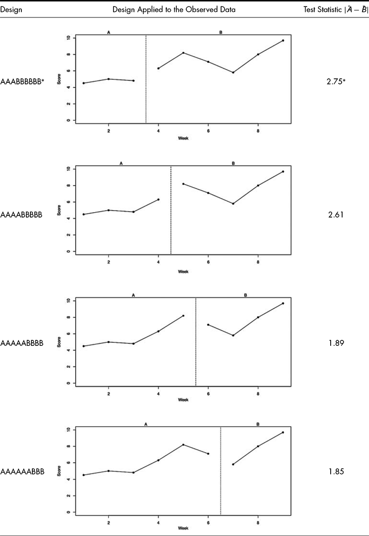
Secondly we have to count the number of possible designs. In this example there are only four possibilities (four possible intervention weeks). Under the null hypothesis that there is no difference between A and B, the same data were observed regardless of the design that would have been applied. In technical terms: the data are fixed and the design is random. If we now calculate the test statistic for each of the possible designs, given the observed data, we obtain a reference distribution for the test statistic. Table 8 shows the test statistic values for each of the four designs and the designs applied to the observed data.
Reference Distribution for the Randomisation Test with
 $| {\bar{A} - \bar{B}} |$
as the Test Statistic Applied to the Data of Samantha in Table 1

*Actually used design and value of the test statistic for the observed data.
Finally, based on this reference distribution, we can calculate the p-value of the randomisation test. This p-value is the proportion of test statistic values in the reference distribution that is equal to or larger than the observed value of the test statistic. For the Samantha data the p-value is .25.
Suppose now that we followed the same procedure for the Thomas data, and that we want to perform a meta-analysis by combining both p-values. Assuming random determination of the start of the B-phase and a minimum of three weeks in each phase, the randomisation test p-value for the Thomas data turns out to be .20. Edgington's (Reference Edgington1972) additive method for combining both p-values results in a combined p-value of (.20 + .25)²/2 = .1013. This result is comparable to the treatment effect p-value of .1141 in Model 5 of the multilevel meta-analysis. Notice, however, that we did not make any assumption regarding random sampling or the shape of the population distribution to justify the calculation of this combined p-value. The simplicity, versatility and freedom from distributional assumptions makes p-value combining an attractive alternative (or addition) for SCE meta-analysis. More information about methods for p-value combining can be found in Rosenthal (Reference Rosenthal1978), Strube and Miller (Reference Strube and Miller1986), Pesarin and Salmaso (Reference Pesarin and Salmaso2010) and Solmi and Onghena (Reference Solmi and Onghena2014). Software to perform randomisation tests for SCEs and to combine p-values is provided by Bulté and Onghena (Reference Bulté and Onghena2008, Reference Bulté and Onghena2009, Reference Bulté and Onghena2013).
Methods for multilevel meta-analysis on the one hand and methods for randomisation tests and p-value combining on the other hand may seem antithetical, with the first being firmly rooted in model-based inference and the latter being the prototype of design-based inference (Koch & Gillings, Reference Koch, Gillings, Johnson and Kotz1984; Sterba, Reference Sterba2009). However, both methods can also be integrated by realising that the randomisation test is not a ‘test’ in the strict sense (because the design and the test statistic are unspecified) but rather a very generic procedure to construct a reference distribution. Consequently, this generic procedure can also be put at work to calculate the p-value of the treatment effect parameter in a multilevel meta-analytic model for SCEs. This so-called ‘randomisation-test wrapper’ can turn any p-value based on parametric assumptions into a design-based p-value based only on random assignment (Cassell, Reference Cassell2002; Heyvaert et al., Reference Heyvaert, Hannes and Onghena2017).
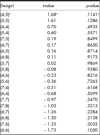
Application of the randomisation test wrapper to the Samantha-Thomas data implies that we have to perform the multilevel meta-analysis 20 times, assuming that both SCEs have a randomly determined start of the B phase and that each phase lasts at least for three weeks. Under those assumptions there are five possible Thomas designs for each of four possible Samantha designs, and a multilevel meta-analysis can be carried out for each constellation of possible start weeks of the B phase. The reference distribution for this randomisation test wrapper is shown in Table 9. There are two test statistics with an absolute value larger than or equal to the observed statistic, and therefore the resulting p-value is 2/20 = .10, which again is comparable to the treatment effect p-value of .1141 in the parametric analysis of Model 5 and the combined p-value of .1013.
Reference Distribution for the Randomisation Test Wrapper with the t-value or the p-value of the treatment effect parameter γ1 of Meta-Analytical Model 5 as the Test Statistic, Applied to the Combined Data of Samantha and Thomas in Tables 1 and 2

†Designs are named according to the start week of the B phase for (Samantha; Thomas).
*Actually used design, test statistic, and p-value for the observed data.
Although randomisation tests and the randomisation test wrapper are useful tools for design-based analysis and meta-analysis of SCEs, notice that they are only relevant for statistical inference regarding treatment effects. Because both procedures are based on random assignment, it is only for the manipulated variable that a reference distribution is generated. General time trends or variation between patients remain invariant under random assignment in replicated SCEs and therefore design-based inference is not possible for the corresponding parameters.
Finally, it should be mentioned that the foregoing presentation of randomisation procedures was framed in terms of null hypothesis testing, but that also confidence intervals can be constructed based on the random assignment rationale. Michiels, Heyvaert, Meulders, and Onghena (Reference Michiels, Heyvaert, Meulders and Onghena2017) showed how to derive confidence intervals for single-case effect size measures by inverting the randomisation test, assuming random assignment and a constant additive treatment effect. Michiels and Onghena (Reference Michiels and Onghena2017) extended this derivation to a collection of SCEs.
Discussion
In this article we presented a unilevel approach for the analysis of SCE data and a multilevel approach for the meta-analysis of multiple SCEs, and we referred to a number of alternative and complementary approaches. Furthermore, we illustrated the unilevel approach, the multilevel approach, probability combining, and the randomisation test wrapper with data from a study by Douglas et al. (Reference Douglas, Knox, De Maio and Bridge2015) on the effectiveness of a new treatment that is intended to strengthen communication-specific coping after traumatic brain injury. Although there are as many approaches to the meta-analysis of SCEs as there are approaches to meta-analysis, we believe that the multilevel approach provides a versatile, flexible, and comprehensive framework for the meta-analysis of SCEs, and that it enables the single-case researcher to connect to general statistical theory (Araujo, Julious, & Senn, Reference Araujo, Julious and Senn2016; Beretvas & Chung, Reference Beretvas and Chung2008; Kratochwill & Levin, Reference Kratochwill and Levin2014; Shadish, Reference Shadish2014; Shadish, Kyse, & Rindskopf, Reference Shadish, Kyse and Rindskopf2013).
With our re-analysis of the data from the Douglas et al. (Reference Douglas, Knox, De Maio and Bridge2015) study, we did not have the intention to be overly critical with respect to the main conclusions of their study. On the contrary, we selected this study because it tackled an important research question, and because its report was very clear, instructive, and transparent regarding data collection, data handling and data analysis. We acknowledge that, in drawing their conclusions, Douglas et al. (Reference Douglas, Knox, De Maio and Bridge2015) linked their precious empirical results to substantive theory, qualitative information about the patients, their treatment, and their follow-up. At the same time, the Douglas et al. (Reference Douglas, Knox, De Maio and Bridge2015) study enabled us to point out the hazards of basing conclusions on short time series and a limited number of patients.
In confronting statistical models with real data, statisticians often have to make concessions and seek ad hoc solutions. Data are frequently more ‘messy’ than the statistical models allows for. On the one hand, a general advice to single-case researchers would be to more carefully design SCEs and to more reliably collect the data. On the other hand, real life usually is messy, certainly when you are working in a hospital. When working with patients with brain injury, unplanned events happen. For example, the Samantha data in the Douglas et al. (Reference Douglas, Knox, De Maio and Bridge2015) study unexpectedly contained one missing week (Table 1) and a thorough statistical analysis should take missing data points into account. We refrained from going into the problems associated with this missing data point because it was not the main purpose of the illustration. However, it is obvious that the increased uncertainty due to the missing data point makes the treatment effect in the Samantha data even less convincing than it already is. Statistical options to formally handle missing data include full maximum likelihood estimation (Hartley & Hocking, Reference Hartley and Hocking1971), multiple imputation (Little & Rubin, Reference Little and Rubin1987), or random assignment if it can be assumed that the missingness is unrelated to the treatment (Edgington & Onghena, Reference Edgington and Onghena2007).
As mentioned before, it is recommended to perform a sensitivity analysis by comparing analyses without the missing data and analyses with techniques to deal with the missing data. If SCEs contain short time series with a lot of missing data, or if SCEs contain messy data in general, the researcher should be reminded of Fisher's (Reference Fisher1938) warning: ‘To consult the statistician after an experiment is finished is often merely to ask him to conduct a post mortem examination. He can perhaps say what the experiment died of’ (Fisher, Reference Fisher1938, p. 17).
Another simplification that we introduced in our analysis of the Douglas et al. (Reference Douglas, Knox, De Maio and Bridge2015) data is that we ignored the results from the follow-up phase. It would have been easy to accommodate the multilevel model for a second A phase (see e.g., Moeyaert et al., Reference Moeyaert, Ugille, Ferron, Onghena, Heyvaert and Van den Noortgate2015) and also randomisation tests for ABA designs are straightforward (see e.g., Onghena, Reference Onghena1992), but as we indicated before, the description of the Douglas et al. (Reference Douglas, Knox, De Maio and Bridge2015) design as an ABA design may not have been the best choice. The design should have been labelled ‘AB with follow-up’. Because the time intervals in the follow-up phase are completely different as compared to the A and B phase, it would have been difficult to include this phase in the multilevel meta-analysis without invoking additional implausible assumptions. Note also that the reference to ABA designs or to reversal or withdrawal designs in some publications might be a side effect of not allowing properly conducted AB designs with extensive follow-up as valid designs (see comment 6 of the SCE definition).
In the example, the multilevel meta-analysis, the p-value combining, and the randomisation test wrapper resulted in comparable p-values for the treatment effect. This in no way suggests that this will always happen. On the basis of this result, it might also be tempting to embark on simulation studies to compare the power and robustness of the different methods, but it is more realistic to consider the different methods being different perspectives for looking at the same data. A combined use of these methods and convergent results strengthen the inference.Footnote 7 For example, a researcher may start the analysis with a bare-bones approach of randomisation tests and p-value combining and may continue with more sophisticated statistical modelling, such as a multilevel meta-analysis, if more time and resources become available. If there are doubts about the parametric assumptions of the multilevel meta-analysis or a design-based inference is needed then the randomisation test wrapper may come into play. Notice also the ‘as if’ nature of the statistical inference in the example because neither random sampling nor random assignment were present. The multilevel meta-analysis is carried out ‘as if’ the two patients were a random sample of the target population and the repeated measurements were a random sample from the patients. The randomisation test and the randomisation tests wrapper are carried out ‘as if’ the start week for the B phase was randomly determined.
We want to end this discussion section with some general comments on the literature regarding the statistical analysis and meta-analysis of SCEs, on statistical modelling, on meta-analysis, and give some suggestions for future research.
Comment on the Literature Regarding the Analysis and Meta-Analysis of SCEs
When reviewing the literature regarding the analysis and meta-analysis of SCEs, one sometimes gets the impression that the wheel is reinvented. Sometimes it seems that a completely new statistical language is needed with specific overlap measures and inferential techniques. In other publications, statistical techniques seem to be borrowed, and at the same time divorced, from the mainstream statistical literature. These techniques might get nourished in particular niche journals with minor reference to the broader statistical literature, but this is not beneficial for the methodological development of the field.
By contrast, in this article we showed that standard multilevel analysis, common meta-analytical tools, and old school randomisation tests can be used for the analysis and meta-analysis of SCEs. The underlying tenet of our demonstration is an advocacy to connect to the general statistical literature and to consider an SCE data set as any other data set. The only special consideration refers to the specific features that all SCE data have in common: repeated observations or measurements and a manipulated variable with at least two levels. These features imply that particular attention has to be paid to time trends and problems of serial dependence, and that randomisation schedules should be compatible with the phasic or alternation structure of the design.
Connecting the analysis and meta-analysis of SCEs to the general statistical literature has the advantage that more than a century of statistical experience and research is made to bear on these data, and that the results of analyses and meta-analyses of SCEs might become more acceptable/ digestible/convincing to the general scientific community. Furthermore, this connection avoids having to repeat all discussions and controversies regarding model-based versus design-based inference, population versus causal inference, frequentist versus Bayesian inference, parametric and non-parametric inference, the complementarity of visual and statistical techniques, the justified use of exploratory and confirmatory techniques, the combination of quantitative and qualitative data, . . . within an isolated SCE community.
Comments on Statistical Modelling
We already indicated that statistical modelling involves making concessions. These concessions are a consequence of any scientific model being an attempt at providing an insightful reduction of a complex reality, guided by the epistemological principle of parsimony. Furthermore, if this principle is left aside, then statistical modelling might become problematic for trustworthy inferences. For example, the multilevel model is so flexible and has so many options that very complex models can be built, to the extent that the model is just a description of the data. This is exactly what happens if the number of parameters to be estimated equals the number of independent data points.
A corollary of this flexibility is that many decisions have to be made in the modelling enterprise and that some decisions might be guided by the researcher's biases pro or contra certain hypotheses. To counteract these biases, and to control for type I and type II errors in a formal statistical framework, it is necessary to specify the model and its test statistics before the data are inspected. Consequently, it might also be recommended for the SCE community to install formal preregistration of SCEs and their meta-analyses (see e.g., the PROSPERO registry; Booth et al., Reference Booth, Clarke, Dooley, Ghersi, Moher, Petticrew and Stewart2012) to steer clear of too many ‘researcher degrees of freedom’ and of too much opportunistic, misguided and self-deceiving post factum model building (Simmons, Nelson, & Simonsohn, Reference Simmons, Nelson and Simonsohn2011; Wicherts et al., Reference Wicherts, Veldkamp, Augusteijn, Bakker, van Aert and van Assen2016).
Comments on Meta-Analysis
According to Eysenck (Reference Eysenck1978) a meta-analysis is ‘an exercise in mega-silliness’ and he referred to a meta-analysis that was, in his opinion, a compilation of heterogeneous (‘mixing apples and oranges’) and poorly designed studies (‘garbage in, garbage out’). Furthermore, meta-analysis is also sometimes contested as a valid scientific method because the results in the sampled or published studies are most likely unrepresentative of the phenomenon studied (the so-called ‘file drawer problem’), meta-analysis conclusions can disagree with large-scale randomised controlled trials, meta-analyses are not reproducible, meta-analyses are performed poorly, and meta-analyses use inferior statistical tools (Borenstein, Hedges, Higgins, & Rothstein, Reference Borenstein, Hedges, Higgins and Rothstein2009; Lakens, Hilgard, & Staaks, Reference Lakens, Hilgard and Staaks2016; Scargle, Reference Scargle2000; Terrin, Schmid, Lau, & Olkin, Reference Terrin, Schmid, Lau and Olkin2003).
This controversy and skepticism regarding meta-analysis carries over to the meta-analysis of SCEs. While some of the criticisms can easily be debunked (see Borenstein et al., Reference Borenstein, Hedges, Higgins and Rothstein2009, and Cooper et al., Reference Cooper, Hedges and Valentine2009, for excellent responses), single-case researchers should be encouraged to raise the bar with respect to the quality of their meta-analyses. The criticism of ‘garbage in, garbage out’ can be turned into a constructive approach to meta-analysis as ‘waste management’ by using methodological and reporting quality of the SCEs as inclusion criteria or moderator variables. Or more fundamentally, single-case researchers can engage in ‘sustainable research’ by producing less waste and improve the overall quality of the design and analysis of the primary studies. The instrument developed by Tate et al. (Reference Tate, Aird and Taylor2013) for the assessment of the methodological quality of SCEs and the reporting guidelines developed by Tate et al. (Reference Tate, Perdices, Rosenkoetter, McDonald, Togher, Shadish and Vohra2016a, Reference Tate, Perdices, Rosenkoetter, Shadish, Vohra, Barlow and Wilson2016b) are very useful in this respect. By paying more attention to the methodological and reporting quality of the primary studies, the field of SCEs as a whole will benefit (Kratochwill et al., Reference Kratochwill, Hitchcock, Horner, Levin, Odom, Rindskopf and Shadish2010, Reference Kratochwill, Hitchcock, Horner, Levin, Odom, Rindskopf and Shadish2013; Lobo, Moeyaert, Cunha, & Babik, Reference Lobo, Moeyaert, Cunha and Babik2017). In addition, the methodological and reporting quality of the SCE meta-analyses, as such, can be improved by adhering to the general standards and guidelines for meta-analyses and systematic reviews (Moher, Liberati, Tetzlaff, Altman, & the PRISMA group, Reference Moher, Liberati, Tetzlaff and Altman2009; Shea et al., Reference Shea, Hamel, Wells, Bouter, Kristjansson, Grimshaw and Boers2009).
Besides the general controversy and skepticism regarding meta-analysis, two concerns need special care when considering an SCE meta-analysis. The first concern is the relatively high risk for selectivity of cases submitted and published in the literature. If cases are published with a strong preference for spectacular, extreme, or successful cases, then any meta-analysis of these cases will be severely biased in the direction of success. A survey by Shadish, Zelinsky, Vevea, and Kratochwill (Reference Shadish, Zelinsky, Vevea and Kratochwill2016) found indications that the publication bias is larger for SCEs than for other research designs indeed. This raises important concerns with respect to the validity of SCE meta-analyses because no sophisticated statistical analysis can remedy the selectivity of cases.
Another concern is the kind of inference that is aimed at with an SCE meta-analysis. As mentioned in our reflection on the definition of an SCE, some SCEs are performed just for the benefit of a single patient (comment 5). Such SCEs are purely idiographic and do not have the intention to be generalisable. They aim at causal inference for one particular patient. When performing an SCE meta-analysis this should be taken into account. It should be clear to what extent the meta-analysis considers the patients as a random sample from a target population and to what extent the meta-analysis is an aggregation for causal inference, with generalisation based on non-statistical arguments.
Future Research
The analysis and meta-analysis of SCEs represents a thriving part of current methodological and statistical developments and applications. In the context of this article, we mention three topics that need more research than currently available.
The first topic is the number of patients and the number of studies needed to perform a reliable and efficient multilevel meta-analysis. Cools, Van den Noortgate, and Onghena (Reference Cools, Van den Noortgate and Onghena2008, Reference Cools, Van den Noortgate and Onghena2009) developed general software to determine the efficiency of multilevel designs, but a validation in the context of SCE meta-analysis is still lacking. It is to be expected that there are numerous factors involved in determining the appropriate number of patients and studies (e.g., the number of repeated measurements and the size of the effects that are considered clinically relevant) but more guiding principles would be useful. Van den Noortgate and Onghena (Reference Van den Noortgate and Onghena2007) suggested that multilevel meta-analysis of SCEs should include at least about 20 entities at the highest level (patients or studies). Also Kuppens et al. (Reference Kuppens, Heyvaert, Van den Noortgate and Onghena2011) recommended that the initial interim analysis of a sequential single-case meta-analysis should comprise at least about 20 single-case publications including single or multiple cases. By contrast, Heyvaert et al. (Reference Heyvaert, Hannes and Onghena2017) performed an extensive simulation study and found acceptable statistical power values for replicated AB designs with seven patients, 20 repeated measurements each, for both multilevel meta-analysis and probability combining of randomisation test p-values.
A second topic is the combination of SCEs and group-comparison studies in one overall meta-analysis. Although, it would be important for evidence-based practice that all kinds of scientific evidence were given weight in comprehensive systematic reviews, it is not evident how one should proceed. One option is to aim at a quantitative integration of both kinds of evidence. For example, Pustejovsky, Hedges, and Shadish (Reference Pustejovsky, Hedges and Shadish2014) proposed a general framework for defining effect sizes in replicated SCEs that are directly comparable to the standardised mean difference in between-subjects randomised experiments (see Punja et al., Reference Punja, Schmid, Hartling, Urichuk, Nikles and Vohra2016, for an application). Shadish, Rindskopf, and Boyajian (Reference Shadish, Rindskopf and Boyajian2016) found similar results between an SCE meta-analysis and the results of a randomised controlled trial but also mentioned that more work is needed to understand the conditions under which this holds. A second option is to use estimates of between- and within subject variances to convert SCE effect sizes in order to make them comparable to group-comparison study effect sizes, and combining them in a single meta-analysis, as described by Van den Noortgate and Onghena (Reference Van den Noortgate and Onghena2008). A third option is to separately perform the SCE meta-analysis and the group-comparison meta-analysis and to combine the results in a narrative way (looking for convergence, elaboration, or confrontation). The latter option has the advantage that also qualitative case studies can be involved (Heyvaert, Hannes, & Onghena, Reference Heyvaert, Hannes and Onghena2017; Heyvaert, Maes, & Onghena, Reference Heyvaert, Maes and Onghena2013). Future research should examine the potential and pitfalls of these options, both in theory and application.
The third topic is the development of guidelines and standards for the statistical analysis and meta-analysis of SCEs. Many authors have referred to the lack of consensus regarding the statistical analysis and meta-analysis of SCEs (see e.g., Cohen, Feinstein, Masuda, & Vowles, Reference Cohen, Feinstein, Masuda and Vowles2014; Smith, Reference Smith2012), which may even reinforce some researchers in just performing a visual analysis and calculating a simple Percentage of Non-overlapping Data (PND), without any further statistical analysis at all (Horner et al., Reference Horner, Carr, Halle, McGee, Odom and Wolery2005; Kratochwill et al., 2010, 2013; Schlosser, Lee, & Wendt, Reference Schlosser, Lee and Wendt2008; Scruggs & Mastropieri, Reference Scruggs and Mastropieri2013). Hence some guidelines and standards are more than welcome (see Manolov & Moeyaert, Reference Manolov and Moeyaert2017b, for some provisional recommendations).
In developing these guidelines and standards we should not chase the chimera that there is only one optimal way of performing the statistical analysis and meta-analysis of SCEs. Optimality always refers to some criterion, and this criterion in its turn can be the subject of debate. We can emphasise robustness, power, small sample properties, asymptotic properties, unbiasedness, accuracy or some other criterion and depending on the criterion have another preference. As wittingly remarked by John Tukey: ‘the collective noun for a group of statisticians is a quarrel’ (Vallverdú, Reference Vallverdú2016), illustrating that this ‘lack of consensus’ is evident for any non-ritualistic statistical analysis (Tukey, Reference Tukey1969). As Stephen Senn (Reference Senn2017) put it: ‘Consult two medics and you'll get two opinions but consult two statisticians and you could easily get three’ (Senn, Reference Senn2017).
Given the current state of the art, there is only one principle that we want to propose for the development of these guidelines and standards. This principle is the connection of any technique for the analysis and meta-analysis of SCEs to the general statistical literature, as we mentioned before. SCE data sets can be analysed as any other data set, with particular attention to time trends, possible serial dependence, and randomisation schedules that are consistent with specific single-case designs. This guiding principle implies a critical attitude towards an overreliance on visual techniques and PND to analyse and meta-analyse SCEs. For example, no one would seriously consider using PND to compare two groups of a randomised controlled trial. For some strange reason, though, we tend to accept this measure for the analysis and meta-analysis of SCEs, although it does not take into account any of the specific features of SCEs.
Conclusion
Patients enter a clinic or a controlled trial one by one and the analysis and meta-analysis of the patients’ data can mimic this data collection procedure. This may be accomplished by testing treatment effects at the individual level first, and subsequently perform a meta-analysis on the collection of individual patient data. For testing treatment effects at the individual level, researchers are recommended to set up SCEs, using the most rigorous experimental procedures possible, given the research setting and resources. In this paper, we presented this bottom-up individualised experimental approach as a viable alternative to the more common group-comparison approach.
In order to select techniques for the analysis and meta-analysis of the SCEs’ data, it is important to have an unambiguous SCE definition at our disposal and to identify the essential features of SCE data. We defined SCEs as ‘true’ experimental studies (i.e., we do not consider them as ‘quasi-experiments’), in which one entity is observed repeatedly under different levels of at least one manipulated variable, with the single entity and the experimental nature as the essential features. For the analysis and meta-analysis of SCEs particular attention has to paid to trends, serial dependence, and the specific single-case design that has been used. The multilevel model, as elaborated in this paper, is particularly suited to deal with the analysis and meta-analysis of SCEs, but other techniques are possible. One other technique, the calculation of PNDs and averaging PNDs, is not recommended because this technique is not geared towards any of the specific features of SCE data.
Sometimes SCE data are messy and sparse and in those cases the appropriate use of multilevel models may be a difficult balancing act. Multilevel models can be very flexible, but they also entail statistical assumptions. So if the design and data are simple or contain all sorts of artefacts, the use of complex multilevel modelling might resemble the use of cannon to kill a fly (and miss it). Other techniques, such as probability combining and the randomisation test wrapper, might be more resilient to the hazards of data collection in clinical practice with brain injured patients, but also these techniques have their shortcomings. The randomisation test wrapper has a sound theoretical foundation, but hitherto applications and investigation of its operating characteristics are lacking. Probability combining is backed by a long history of statistical research, but is only subsidiary in the context of a meta-analysis because it does not provide an effect size estimate and may mask effects that go in opposite directions if the use of one-sided or two-sided p-values is not appropriately specified (Borenstein et al., Reference Borenstein, Hedges, Higgins and Rothstein2009; Edgington & Onghena, Reference Edgington and Onghena2007).
With respect to the number of patients for a proper use of multilevel meta-analysis of SCEs, single-case researchers should not settle for a small number of patients, each providing a small number of repeated measurements. The use of multilevel models requires the number of patients and the number of repeated measurements based on a corresponding statistical power analysis. In any case, single-case researchers are encouraged to justify their sample of patients and to be wary of indications of publication and reporting biases. If no other justification is available, it is safest to follow the tentative recommendations proposed by Kratochwill et al. (2010, 2013) and to refrain from meta-analysing published SCEs with the intention to derive a general causal effect unless the following criteria are met:
-
1. A minimum of five SCE research papers, using valid experimental designs,
-
2. A minimum of three different research teams at three different geographical locations who conducted the SCEs, and
-
3. A minimum of 20 SCEs across the papers.
Finally, one meta-conclusion after reviewing the literature on SCE meta-analysis: The single-case research community would benefit from more unified terminology and methodology. For example, the emergence of terms such as ‘N-of-1 trial’ and ‘Individual Participant Data meta-analysis’ has created dissociated literatures with little or no cross-references to the original publications on SCEs and SCE meta-analysis. For the future of SCE analysis and meta-analysis, we hope that this can be remedied and that more cross-fertilisation will occur. It is not because another word is used, that another reality is represented.
Acknowledgements
We want to thank the guest editor, Robyn Tate, and two anonymous reviewers for their helpful suggestions regarding a previous version of this manuscript.
Financial Support
This work was supported by the Research Foundation – Flanders (FWO), Belgium (P.O., Grant number K8.017.15N), (B.M., Grant number G.0593.14); and by the Institute of Education Sciences, U.S. Department of Education (L.J., M.M. and W.V.d.N., Grant number R305D150007). The opinions expressed are those of the authors and do not represent views of the Research Foundation – Flanders or the U.S. Department of Education.
Conflict of Interest
Patrick Onghena has no conflicts of interest to disclose. Bart Michiels has no conflicts of interest to disclose. Laleh Jamshidi has no conflicts of interest to disclose. Mariola Moeyaert has no conflicts of interest to disclose. Wim Van den Noortgate has no conflicts of interest to disclose.
Ethical Standards
The authors assert that all procedures contributing to this work comply with the ethical standards of the relevant national and institutional committees on human experimentation and with the Helsinki Declaration of 1975, as revised in 2008.
Supplementary Materials
To view supplementary material for this article, please visit https://doi.org/10.1017/BrImp.2017.25.