


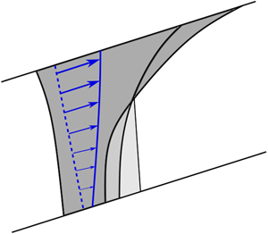





1. Introduction
Carbon capture and storage (CCS) is one of the key technologies for reducing CO $_{2}$ emissions in the short and medium term. CCS involves capturing carbon dioxide, compressing it and then transporting it to storage sites where it is sequestered in geological formations one to two kilometres below the surface (Bickle Reference Bickle2009). In the UK, the current government target is to capture and store 20 Mt CO
 $_{2}$ per year by 2035 and 100 Mt CO
 $_{2}$ per year by 2050 (Gummer Reference Gummer2018).
One of the major challenges for the deployment of CCS is determining the volume of CO $_{2}$ that can be stored safely in a particular target geological strata or ‘reservoir’. Often the geological strata are characterised by laterally extensive, but relatively thin layers of permeable rock, saturated with brine and overlaid by a layer of very low permeability, called a seal rock. Many target reservoirs have anticline structures, so that the buoyant CO
 $_{2}$ can collect below the seal rock at the crest of the formation, displacing the brine downwards. However, in some cases the permeable layer has a small inclination which extends over a very large distance. In this case, a plume of buoyant CO
 $_{2}$ will gradually migrate updip, with a small fraction (known as the residual saturation) of the CO
 $_{2}$ being trapped by capillary forces as the tail of the flow is displaced upwards by the formation water. This so-called capillary trapping is a key stage in the geo-sequestration process, since the plume of CO
 $_{2}$ eventually becomes immobile (Hunt, Sitar & Udell Reference Hunt, Sitar and Udell1988; Hesse, Orr & Tchelepi Reference Hesse, Orr and Tchelepi2008; Bickle Reference Bickle2009). The fraction of the pore space in the target reservoir which actually traps the CO
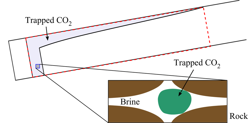
 $_{2}$ is critical for efficient use of the reservoir and is therefore a source of considerable interest (see figure 1). It is very challenging to increase the efficiency of the storage because the CO
 $_{2}$ is buoyant and very mobile and so tends to focus just below the upper boundary of the target reservoir, bypassing much of the pore space below (Hesse et al. Reference Hesse, Orr and Tchelepi2008). To date many assessments of the fraction of the pore space which can be accessed by the plume have been based on the assumption that the flow properties of the geological strata are constant in space. However, many sedimentary deposits are formed by the deposition of particles from suspension flows, and the intensity and particle load in these flows varies in time as the flows either wax or wane (e.g. Kneller & McCaffrey Reference Kneller and McCaffrey2003; Dennielou et al. Reference Dennielou, Huchon, Beaudouin and Berné2006). As a result, the layers may be vertically graded in mean grain size
 $d$, and this leads to vertical gradients in the permeability, which depends on
 $d^2$ as well as the variance in the grain size, amongst other factors (Allen Reference Allen1960; Dullien Reference Dullien2012). With vertical changes in grain size of a factor of 2–3, we expect permeability changes of a factor of 4–9 across one element of the geological strata; curiously, the porosity of the formation is much less sensitive to these changes in grain size (e.g. figure 13 in Fitch et al. Reference Fitch, Lovell, Davies, Pritchard and Harvey2015). The vertical grading may extend over a significant lateral scale owing to the formation of such sedimentary layers from sustained suspension flows. Such changes in permeability may have a significant impact on the velocity structure of the CO
 $_{2}$ plume as it migrates updip (Hinton & Woods Reference Hinton and Woods2018, Reference Hinton and Woods2019), and in turn this may impact the fraction of the pore space in the geological strata accessed by the plume. In some geological formations, variations in the permeability may also arise from post-depositional reactions, for example associated with the dolomitisation reaction produced by a gravitational intrusion of sea-water into a carbonate deposit, or through reactions associated with hydrothermal circulation, which can lead to preferential reaction near the top or the base of the formation (Verdon & Woods Reference Verdon and Woods2007; Phillips Reference Phillips2009). It is the purpose of this paper to explore the impact of such permeability gradients on the efficiency of capillary trapping as a plume migrates updip in a reservoir of finite vertical extent and which is bound above and below by less permeable seal layers in the geological strata (see figure 2).
Schematic of the trapped CO $_{2}$ when the plume has become immobilised. The region that is swept by the CO
 $_{2}$ is shaded. This pore space is not entirely occupied by CO
 $_{2}$, as shown in the zoomed-in box. It is trapped and surrounded by ambient brine.
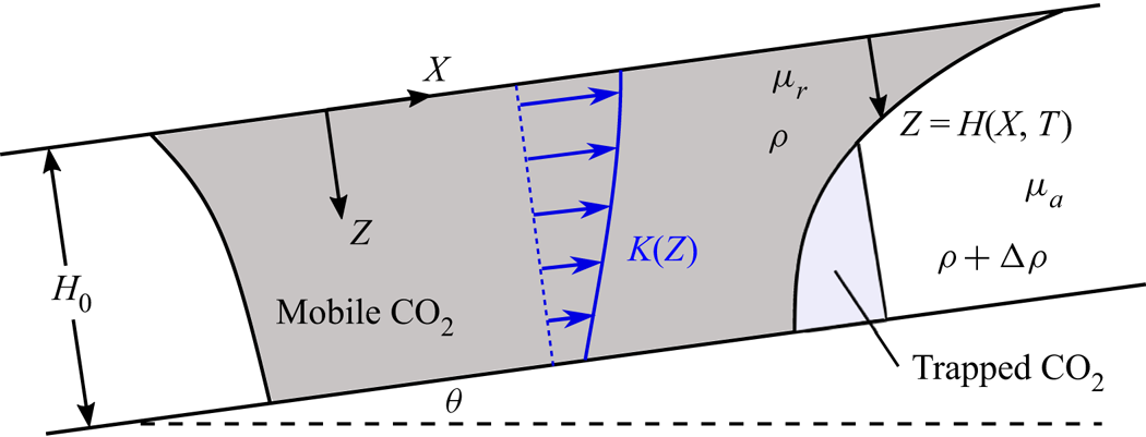
Schematic diagram showing the migration of buoyant CO $_{2}$ in an inclined, confined layer of porous rock with vertically varying permeability.
We build from the existing and substantial literature on this topic, but which has largely focussed on capillary trapping in homogeneous reservoirs, and we compare the present results with these earlier models as a reference. In an inclined layer which is bounded only by a seal layer at the top, the motion of the ambient fluid is unimportant, and simple estimates of the run-out time and distance have been obtained (Woods Reference Woods2014). In horizontal (and nearly horizontal) layers, Kochina, Mikhailov & Filinov (Reference Kochina, Mikhailov and Filinov1983) found similarity solutions of the second kind for the evolution of the plume as it is gradually trapped. The volume of the mobile CO $_{2}$ evolves as a power law function of time where the exponent in the power law depends on the fraction of the pore space in which CO
 $_{2}$ is trapped. Our modelling provides a quantitative basis for assessing the impact of vertical permeability grading on the efficiency of sequestration and may lead to new technical solutions to enhance access to the pore space. Indeed, it has been shown that in a homogeneous reservoir, the initial injection phase, which determines the structure and shape of the mobile CO
 $_{2}$, has an important impact on the trapping efficiency (Kochina et al. Reference Kochina, Mikhailov and Filinov1983; Juanes et al. Reference Juanes, Spiteri, Orr and Blunt2006; MacMinn & Juanes Reference MacMinn and Juanes2009), and so we explore the combination of this effect with the vertical gradient in permeability. Generally, increasing the injection rate leads to a more localised injection plume, and this may reduce the run-out distance. Thus more CO
 $_{2}$ may be stored if the fluid is injected at a higher rate (cf. Bachu Reference Bachu2015). In addition, other models have included a background hydrological flow and shown that this may enhance the rate of trapping as the post-injection plume migrates through the layer (Juanes, MacMinn & Szulczewski Reference Juanes, MacMinn and Szulczewski2010; MacMinn, Szulczewski & Juanes Reference MacMinn, Szulczewski and Juanes2010).
There are many other processes which arise during the sequestration of CO $_{2}$ including dissolution into the ambient brine (Riaz & Cinar Reference Riaz and Cinar2014) and leakage into the seal layer (Farcas & Woods Reference Farcas and Woods2009). It has previously been shown that dissolution may have a significant effect on the storage efficiency (MacMinn, Szulczewski & Juanes Reference MacMinn, Szulczewski and Juanes2011; MacMinn & Juanes Reference MacMinn and Juanes2013). Also, transverse flow (into the page in figure 1) may reduce the extent of the CO
 $_{2}$, especially if the transverse extent of the initial plume is small relative to its updip extent. Since we are interested primarily in understanding the importance of vertical variations in permeability on the storage efficiency, we present a two-dimensional model and neglect transverse flow and dissolution in our initial analysis. However, we reintroduce these effects later in the manuscript and demonstrate that although they change the behaviour, our results and principles concerning the influence of heterogeneity are robust to the inclusion of these additional processes.
We note that when the plume becomes very thin, the capillary entry pressure may prevent the mobile CO $_{2}$ spreading further (Zhao et al. Reference Zhao, MacMinn, Huppert and Juanes2014). However, it is often the case that this entry pressure is very small compared to the hydrostatic pressure and so the effect may be neglected; we assume this henceforth (Hesse et al. Reference Hesse, Orr and Tchelepi2008).
In § 2 we formulate the model for the post-injection evolution of the CO $_{2}$ plume including capillary trapping at the receding CO
 $_{2}$–brine interface. We assume the displacement is slow enough that the gravity–capillary equilibrium is maintained in any vertical cross section and that there is a sharp interface between the CO
 $_{2}$ and the brine, which is valid provided that the layer thickness is large compared to the capillary transition zone (e.g. Hesse et al. Reference Hesse, Orr and Tchelepi2008). The governing equation is integrated numerically, and the results demonstrate that at late times the role of buoyancy across the layer is negligible. This motivates the asymptotic analysis of § 3 in which we consider the release of a rectangle of CO
 $_{2}$ and neglect the diffusive term, which is equivalent to assuming the initial release has a small aspect ratio. This provides a set of reference calculations that illustrate the influence of a linear cross-layer permeability variation on the run-out distance. The asymptotic analysis identifies the different stages of migration of the CO
 $_{2}$ and how these are controlled by the parameters in the problem, such as the permeability variation across the layer. We also include dissolution and three-dimensional effects in §§ 3.3, 3.4. In § 4, we study the role of the initial distribution of the CO
 $_{2}$, which is characterised by the dimensionless injection flux. Finally, the implications of our results are explored in § 5. We show that since the storage efficiency is inversely proportional to the run-out distance then in some layers one can compensate for the efficiency reduction associated with an unfavourable permeability gradient by increasing the injection flux.
2. Model
We consider the release of a fixed volume of supercritical CO $_{2}$ with density
 $\rho$ and viscosity
 $\mu _r$ in a porous layer saturated with brine with density
 $\rho + {\rm \Delta} \rho$ and viscosity
 $\mu _a$. The setup is shown in figure 2 where dark grey represents the CO
 $_{2}$, light grey represents the trapped CO
 $_{2}$ and white represents the brine. The
 $X$ and
 $Z$ axes are defined as shown in figure 2 with the top of the layer corresponding to
 $Z=0$. The layer has thickness
 $H_0$, is bounded above and below by impermeable layers and is inclined at an angle
 $\theta$ to the horizontal. The absolute permeability,
 $K(Z/H_0)$, varies with depth and the porosity,
 $\phi$, is constant. The presence of the ambient brine reduces the effective permeability of the CO
 $_{2}$ by a factor,
 $k_r$, known as the relative permeability. Likewise the flow of the ambient brine is inhibited by the CO
 $_{2}$, and we denote its relative permeability by
 $k_a$. We assume that the interface between the fluids at
 $Z=H(X,T)$ is sharp. There can be intermingling of the fluids especially at the leading edge of the plume, but previous experimental studies have shown that the mixing region is relatively small, and elsewhere a sharp interface model is accurate (Golding & Huppert Reference Golding and Huppert2010; Pegler, Huppert & Neufeld Reference Pegler, Huppert and Neufeld2014).
Provided that the horizontal lengthscale is much larger than the layer thickness,  $H_0$, the pressure in the injected and ambient fluids is hydrostatic and given by (Bear Reference Bear1971)
 \begin{equation} P(X,Z,T)= \left\{\begin{array}{@{}ll} P_0(X)+ \rho g Z \cos \theta +P_c & 0 \lt Z \lt H \\ P_0(X) + (\rho + {\rm \Delta} \rho) g Z \cos \theta - {\rm \Delta} \rho g H \cos \theta & H \lt Z \lt H_0, \end{array}\right. \end{equation}
where  $P_0(X)$ is the unknown pressure at the top boundary (
 $Z=0$) and
 $P_c$ is the constant capillary pressure. The Darcy flux per unit height in the injected and ambient fluids is given by
 \begin{gather} U_r = -\lambda_r \bar{K} k (Z/H_0) \left[\frac{\partial P_0}{\partial X} + \rho g \sin \theta \right], \end{gather}
 \begin{gather}U_a = -\lambda_a \bar{K} k (Z/H_0) \left[\frac{\partial P_0}{\partial X} - {\rm \Delta} \rho g \cos \theta \frac{\partial H}{\partial X} + (\rho + {\rm \Delta} \rho) g \sin \theta \right], \end{gather}
respectively, where  $\lambda _r=k_r/\mu _r$ and
 $\lambda _a=k_a/\mu _a$ are the mobilities of the two fluids and
 $k(Z/H_0)$ is the dimensionless permeability defined relative to the mean permeability,
 $\bar {K}=({1}/{H_0})\int _0^{H_0} K(Z/H_0) \,\mathrm {d} Z$. The unknown pressure gradient,
 $\partial P_0/\partial X$, can be eliminated by applying the constraint that the total net flux in the
 $X$ direction vanishes:
 \begin{equation} \int_0^{H(X,T)} U_r \,\textrm{d} Z + \int_{H(X,T)}^{H_0} U_a \,\textrm{d} Z =0. \end{equation}
The flow rate (2.2) is integrated over the thickness of the injected fluid to obtain the fluxes,  $Q_r$ and
 $Q_a$, in the injected and ambient fluids, respectively,
 \begin{align} Q_r &= -Q_a = \int_0^{H(X,T)} U_r \,\textrm{d} Z \nonumber\\ &= \frac{{\rm \Delta} \rho g \bar{K} H_0}{\mu_r} \frac{m \psi(H/H_0) \left[1- \psi(H/H_0) \right]}{m+(1-m)\psi(H/H_0)} \left(\sin \theta - \frac{\partial H}{\partial X} \cos \theta \right), \end{align}
where
 \begin{equation} m=\frac{\mu_r/k_r}{\mu_a/k_a} \end{equation}
is the mobility ratio and
 \begin{equation} \psi(H/H_0) =\frac{1}{H_0} \int_0^H k(Z/H_0) \,\textrm{d} Z \end{equation}
is the depth-integrated permeability.
To obtain an equation for the evolution of the interface, we consider local mass conservation in the CO $_{2}$ phase,
 \begin{equation} \hat{\phi} \frac{\partial H}{\partial T} = -\frac{\partial Q_r}{\partial X}, \end{equation}
where the effective porosity,  $\hat {\phi }$, is reduced owing to capillary trapping of CO
 $_{2}$ within the pores and takes the following values relative to the porosity of the rock,
 $\phi$:
 \begin{equation} \hat{\phi}=\left\{\begin{array}{@{}ll} \phi(1-S_a-S_r) & \text{for}\ \partial H/\partial T <0 \\ \phi(1-S_a) & \text{for}\ \partial H/\partial T >0, \end{array}\right. \end{equation}
where  $S_{a}$ represents the saturation of immobile ambient fluid left behind as the injected fluid invades the pore space, whilst
 $S_r$ represents the saturation of the CO
 $_{2}$ left behind as the brine invades the region occupied by CO
 $_{2}$. Upon substituting for the flux,
 $Q_r$ in (2.8), we obtain the following advection–diffusion type equation for the shape of the interface,
 $Z=H(X,T)$:
 \begin{equation} \frac{\partial H}{\partial T} = -\frac{{\rm \Delta} \rho g \bar{K}}{\mu_r \hat{\phi}} \frac{\partial}{\partial X} \left\{ \frac{m \psi(H/H_0) \big[1- \psi(H/H_0) \big]}{m+(1-m)\psi(H/H_0)} \left(\sin \theta - \frac{\partial H}{\partial X} \cos \theta \right) \right\}. \end{equation}
We assume that the rock is invaded by the CO $_{2}$ for the first time so the ambient brine is initially unsaturated with CO
 $_{2}$. The horizontal lengthscale of the injected CO
 $_{2}$ is initially
 $X \sim L$ and so we introduce the scaled properties
 \begin{equation} h=H/H_0,\quad x=X/L,\quad t = T/T_0, \end{equation}
where the timescale,
 \begin{equation} T_0 = \frac{\mu_r \phi (1-S_a -S_r)L}{{\rm \Delta} \rho g \bar{K} \sin \theta}, \end{equation}
corresponds to the lengthscale,  $L$, divided by the along-layer buoyancy velocity in the case that the brine displaces the CO
 $_{2}$. The dimensionless governing equation is
 \begin{equation} \sigma^{-1} \frac{\partial h}{\partial t} + \frac{\partial}{\partial x} [g(h)] = \mathcal{F} \frac{\partial}{\partial x} \left[g(h) \frac{\partial h}{\partial x}\right], \end{equation}
where
 \begin{equation} g(h) = \frac{m \psi(h) [1-\psi(h)]}{m+(1-m)\psi(h)} \end{equation}
is the flux function, and
 \begin{equation} \sigma=\left\{\begin{array}{@{}ll} 1 & \text{for}\ h_t <0 \\ 1-\epsilon & \text{for}\ h_t >0, \end{array}\right. \end{equation}
with
 \begin{equation} \epsilon = S_r/(1-S_a) \end{equation}
representing the effect of the capillary trapping of the CO $_{2}$ at the receding edge of the plume. The parameter
 $\epsilon$ is a function of the geometry of the pore space and the interfacial tension between the CO
 $_{2}$, the brine and the mineral surfaces (Bear Reference Bear1971; Lake Reference Lake1989). The parameter multiplying the diffusive term on the right-hand side of (2.13) is
 \begin{equation} \mathcal{F} = \frac{H_0}{L \tan \theta}, \end{equation}
and this quantifies the importance of the component of buoyancy acting perpendicular to the boundary relative to the component acting parallel to the boundary.
In a uniform layer, the permeability functions are  $k(z) \equiv 1$ and
 $\psi (h) \equiv h$, and (2.13) reduces to the governing equation of Hesse et al. (Reference Hesse, Orr and Tchelepi2008). It is also useful to note that
 $\psi (0)=0$,
 $\psi (1)=1$ and hence
 $g(0)=g(1)=0$, which corresponds to zero net flux in the
 $x$ direction. To illustrate the effect of variations in permeability, we use a linear permeability profile,
 \begin{equation} k(z) = 1 + {\rm \Delta} k \left(z-1/2\right), \end{equation}
where  $-2<{\rm \Delta} k <2$ is the permeability difference across the layer relative to the mean permeability. If the permeability in the layer is higher at the top (
 $z=0$) then
 ${\rm \Delta} k < 0$, and if the permeability is higher at the bottom (
 $z=1$) then
 ${\rm \Delta} k >0$. We assume throughout this work that the porosity,
 $\phi$, and the saturations,
 $S_a$ and
 $S_r$ (and hence
 $\epsilon$), are constant in the layer. This is consistent with a varying permeability provided that the pore geometry is constant while the pore size may vary, as has been observed in some porous layers (e.g. figure 13 in Fitch et al. Reference Fitch, Lovell, Davies, Pritchard and Harvey2015).
We note that the dimensionless velocity in the injected fluid is
 \begin{equation} u_r(x,z,t) = \frac{[1-\psi(h)]mk(z)}{m+(1-m)\psi(h)} \left(1-\mathcal{F} \frac{\partial h}{\partial x} \right), \end{equation}
whilst in the ambient fluid, the dimensionless velocity is
 \begin{equation} u_a(x,z,t) = \frac{-\psi(h)mk(z)}{m+(1-m)\psi(h)} \left(1-\mathcal{F} \frac{\partial h}{\partial x} \right). \end{equation}
An example of the velocity profile in the mobile CO $_{2}$ and the ambient brine is shown in figure 3 for
 $h=0.5$ in the case that the permeability increases towards the top boundary (
 ${\rm \Delta} k=-1$) and
 $m=0.2$.


Equation (2.13) is integrated numerically, and details are provided in appendix A. The numerical results in the case of a step function release ( $h=0$ for
 $x>1/2$ and
 $h=1$ for
 $x < 1/2$) are compared to our asymptotic results in figure 4 in the case of no capillary trapping (
 $\epsilon =0$). Each panel corresponds to different values of the mobility ratio,
 $m$, and the permeability gradient,
 ${\rm \Delta} k$. We use three values of the parameter
 $\mathcal {F}$, and results are shown at time
 $t=1$. The asymptotic predictions obtained in § 3, in which the diffusive term in the governing equation (2.13) is neglected, are shown as red dotted-dashed lines. The approximations show good agreement with the numerical results provided that
 $\mathcal {F} \ll 1$. Figures 4(b) and 4(c) demonstrate that the interface may develop a shock-like region of fixed extent at the top or bottom depending on the parameter values and we explore this further in the next section.
The three regimes for the early evolution of the upslope interface. We use  $\epsilon =0$ and
 $t=1$. (a)
 ${\rm \Delta} k =0.5$ and mobility ratio,
 $m=0.3$ (no fixed-extent regions). (b)
 ${\rm \Delta} k =1.5$ and
 $m=0.5$ (fixed-extent region at the top). (c)
 ${\rm \Delta} k =-1$ and
 $m=1$ (fixed-extent region at the bottom).

We have neglected dissolution of the CO $_{2}$ into the ambient brine but reintroduce it in § 3.3 and discuss its importance. Throughout the majority of this paper, we focus on the two-dimensional setup described above. Three-dimensional effects are discussed in further detail in § 3.4.
3. A rectangular release of CO $_{2}$

The post-injection evolution of the plume in the case of varying permeability and capillary trapping is complex and the behaviour may depend sensitively on the initial shape of the plume. Therefore, we begin our analysis by considering the simple idealised initial condition,
 \begin{equation} h=\left\{\begin{array}{@{}ll} 1 & \text{for}\ -1/2 \lt x \lt 1/2\\ 0 & \text{otherwise.} \end{array}\right. \end{equation}
The initial dimensionless volume of the plume is unity. This corresponds to a dimensional volume of  $\phi (1-S_a) H_0 L$. Initial conditions that are more realistic for the context of CO
 $_{2}$ sequestration are considered in § 4. In the present section, we determine the evolution of a plume with initial shape given by (3.1) for reference. We refer to the part of the interface initially at
 $x=1/2$ as the ‘upslope’ interface and the part initially at
 $x=-1/2$ as the ‘downslope’ interface. At early times, the evolution of the two interfaces is independent and we analyse the upslope interface first.
The relative significance of the diffusive term on the right-hand side of (2.13) diminishes as the extent of the plume grows. This motivates asymptotic analysis in which the diffusive term is neglected. The primary aim of this analysis is not to provide precise solutions to the model, which can be provided through numerical integration, but rather to elucidate the key stages and processes in the migration of the plume and their dependence on the parameters in the problem, particularly the permeability variation.
The diffusive term may be neglected when the extent is large ( $x \gg \mathcal {F}$). The very early parabolic behaviour in which the diffusive term dominates is ignored in our asymptotic calculations because the volume that is capillary trapped during this period is negligible (Hesse et al. Reference Hesse, Orr and Tchelepi2008). We seek solutions to the approximate equation
 \begin{equation} \frac{\partial h}{\partial t} + \sigma g'(h) \frac{\partial h}{\partial x} =0, \end{equation}
which is a first-order hyperbolic partial differential equation. We solve (3.2) using the method of characteristics. In  $(x,t)$ space, the lines of constant
 $h$ are given by
 \begin{equation} \frac{\mathrm{d}x}{\mathrm{d} t} = \sigma g'(h) \equiv \sigma \frac{m[1-\psi(h)]^2 - \psi(h)^2}{[m + (1-m)\psi(h)]^2} mk(h). \end{equation}
We note that  $g'(0)>0$ and
 $g'(1)<0$, and initially the upslope interface advances at the top (
 $h=0$) and recedes at the bottom of the layer (
 $h=1$). There is a height,
 $h_0$, at which the interface is stationary, given by the solution to
 $g'(h_0)=0$, which is equivalent to
 \begin{equation} \psi(h_0) = \hat{m} \equiv [ 1 + m^{-1/2}]^{-1}. \end{equation}
For a uniform layer ( ${\rm \Delta} k=0$) we recover the stationary height,
 $h_0 = \hat {m}$ obtained by Hesse et al. (Reference Hesse, Orr and Tchelepi2008). The stationary height is independent of the trapping parameter,
 $\epsilon$.
The interface advances in  $0 < h < h_0$ and recedes in
 $h_0 < h < 1$, and this determines the value of
 $\sigma$ at each height in (3.2). If
 $g'(h)$ is a monotonically decreasing function of
 $h$ in
 $(0,1)$ then the method of characteristics can be applied to obtain the implicit solution to (3.2) everywhere. For a linear permeability profile, the condition that
 $g'(h)$ is monotonically decreasing corresponds to
 \begin{equation} \left.\begin{array}{ll@{}} m < (2-{\rm \Delta} k)^2 / (2 {\rm \Delta} k) & \text{for}\ {\rm \Delta} k \geq 0 \\ m > -2 {\rm \Delta} k/(2+{\rm \Delta} k)^2 & \text{for}\ {\rm \Delta} k < 0 \end{array}\right\} \end{equation}
and in this case, the shape of the upslope interface is given by
 \begin{equation} x=\left\{\begin{array}{@{}ll} 1/2 + (1-\epsilon) g'(h) t & \text{for}\ 0 \lt h \lt h_0,\\ 1/2 + g'(h) t & \text{for}\ h_0 \lt h \lt 1. \end{array}\right. \end{equation}
The advancing portion of the interface is slowed by the reduction in flux associated with capillary trapping at the receding interface. The interface evolves as a growing rarefaction wave, and the solution (3.6) shows good agreement with our numerical results at  $t=1$ for
 $\mathcal {F} \ll 1$ (see figure 4a).
If  $g'(h)$ is not a monotonically decreasing function of
 $h$ in
 $(0,1)$ then the characteristics cross in
 $(x,t)$ space and a discontinuity (i.e. a shock) develops in the upslope interface. There is a shock at the top that includes
 $h=0$ if
 $g''(0)>0$ (see figure 4b). For a linear permeability profile,
 $g''(0)>0$ is equivalent to
 \begin{equation} m > \frac{(2-{\rm \Delta} k)^2}{2 {\rm \Delta} k} \quad \text{and}\quad {\rm \Delta} k >0. \end{equation}
There is a shock at the bottom (see figure 4c) that includes  $h=1$ if
 $g''(1)>0$, which is equivalent to
 \begin{equation} m < \frac{-2 {\rm \Delta} k}{(2+{\rm \Delta} k)^2} \quad \text{and} \quad {\rm \Delta} k <0. \end{equation}
For a linear permeability profile, these are the only two possibilities; an internal shock that does not include  $h=0$ or
 $h=1$ is not possible. The shocks occur when the interface predicted by the flux function,
 $x=g'(h) t$, has a turning point, which arises when the flow velocity at the top (or bottom) of the layer is sufficiently small compared to the mean flow velocity. Therefore, a shock at the top (or bottom) occurs when the permeability is low at the top (or bottom), corresponding to
 ${\rm \Delta} k >0$ (or
 ${\rm \Delta} k < 0$).
The three cases of (a) no shock, (b) a shock at the top of the layer and (c) a shock at the bottom are shown in figure 4 and delineated in parameter space in figure 5.
Parameter space delineating the different shapes of the upslope interface for  $m \leq 1$. The letters correspond to the panels in figure 4.

For the case of zero capillary trapping ( $\epsilon =0$), the height,
 $h_s$, and speed,
 $v_s$, of the shock at the top can be calculated from continuity of the interface at
 $h=h_s$ and a Rankine–Hugoniot condition, associated with mass conservation:
 \begin{equation} v_s = g'(h_s), \quad v_s h_s =g(h_s). \end{equation}
We note that  $v_s>0$ and hence
 $h_s < h_0$ and the shock does not include the stationary height. The shape of the interface can now be obtained for
 $\epsilon \geq 0$:
 \begin{equation} x=\left\{\begin{array}{@{}ll} 1/2 + (1-\epsilon) v_s t & \text{for}\ 0 < h < h_s \\ 1/2 +(1-\epsilon) g'(h) t & \text{for}\ h_s < h < h_0 \\ 1/2 + g'(h) t & \text{for}\ h_0 < h < 1, \end{array}\right. \end{equation}
where  $h_0$ is again the height at which
 $g'(h_0)=0$. This shape is compared to our numerical results in figure 4(b).
We may carry out similar analysis in the case of a shock at the bottom to obtain the equations
 \begin{equation} v_s = g'(h_s),\quad v_s (1-h_s) =-g(h_s), \end{equation}
where the shock lies in  $h \in [h_s, 1]$. The shock velocity,
 $v_s$, is negative and
 $h_s >h_0$. The shape of the interface is (see figure 4c)
 \begin{equation} x=\left\{\begin{array}{@{}ll} 1/2 + (1-\epsilon) g'(h)t & \text{for}\ 0 < h < h_0 \\ 1/2 + g'(h) t & \text{for}\ h_0 < h < h_s \\ 1/2 + v_s t & \text{for}\ h_s < h < 1. \end{array}\right. \end{equation}
We have found three regimes for the evolution of the upslope interface before it interacts with the downslope interface. Our results apply provided that the plume is sufficiently long so that the diffusive term, corresponding to the component of buoyancy acting perpendicular to the boundary, is negligible. We also note that in the case that there is a shock at the top of the layer, which occurs when  ${\rm \Delta} k >0$ and the mobility ratio satisfies (3.7), the buoyant injected fluid may preferentially migrate along the bottom of the layer where the permeability is highest. The introduction of a shock near
 $h=0$ corresponds to a weak solution of the governing equation, and the assumption underlying this solution is that cross-layer buoyancy-driven flow is sufficiently fast that the buoyant injected fluid always lies above the denser ambient fluid. However, if the layer inclination,
 $\theta$, is sufficient, this may not occur and the interface may advance upslope most rapidly in the middle of the layer leading to a possible cross-layer Rayleigh–Taylor type instability and the invalidation of our model. Such behaviour has been observed in layers which partition into two sublayers of differing permeability in the case of an injection-driven flow and an inclined buoyancy-driven flow (Huppert, Neufeld & Strandkvist Reference Huppert, Neufeld and Strandkvist2013; Debbabi et al. Reference Debbabi, Jackson, Hampson and Salinas2018). This instability does not occur in cases with no shock or with a shock at the bottom of the layer, which is associated with the high mobility of the ambient fluid. We now focus the analysis on these two cases; the case of a shock at the top of the layer is included for completeness noting the caveat above.
The downslope interface is initially a line across the layer at  $x=-1/2$. At early times, the interface is stationary because in
 $0 < h < h_0$ the characteristic velocity of the interface (3.3) is upslope and in
 $h_0 < h < 1$ it is downslope, but owing to buoyancy the injected fluid cannot lie below the ambient fluid and hence there is no motion (for further details, see Hesse et al. Reference Hesse, Orr and Tchelepi2008). The early-time approximation of the downslope interface as a stationary line at
 $x=-1/2$ perpendicular to the boundaries is accurate provided that
 $\mathcal {F} \ll 1$ (Gunn & Woods Reference Gunn and Woods2011).
3.1. Interaction with the downslope interface
We next analyse the evolution of the interface after it detaches from the bottom boundary. The downslope interface remains at  $x=-1/2$ until the receding part of the upslope interface collides with it (see figures 6 and 7). The time of this collision,
 $t_1$, is obtained by considering the fastest receding point on the upslope interface. In the absence of a shock at the top of the layer, the fastest point is at
 $h=1$ and the time is given by the solution to
 $1/2 + g'(1)t_1=-1/2$. If there is a shock at the top of the layer then
 $g'(1)$ is replaced by the velocity of the shock. The collision time is given by
 \begin{equation} t_1=\left\{\begin{array}{@{}ll} \big[mk(1)\big]^{-1} & \text{no shock at}\ h=1 \\ -v_s^{-1} & \text{shock at}\ h=1. \end{array}\right. \end{equation}
The injected fluid subsequently detaches from the lower boundary,  $y=1$, and the downslope interface, which is approximated by a line perpendicular to the boundary, begins to move with velocity
 \begin{equation} \frac{\mathrm{d} \mathcal{X}}{\mathrm{d} t} = g(\mathcal{H})/\mathcal{H}, \end{equation}
where  $x=\mathcal {X}(t)$ is the location of the travelling downslope interface and
 $h=\mathcal {H}(t)$ is its thickness. We note that
 $\mathcal {H}(t)$ is the evolving thickness of the downslope interface at the trailing edge of the plume, whereas
 $h_s$ is used to denote the fixed location of a shock in the slumping of the upslope interface, when it occurs. The initial condition for (3.14) is
 $\mathcal {X}(t_1)=-1/2, \mathcal {H}(t_1)=1$ if there is no shock at
 $h=1$ in the upslope interface and
 $\mathcal {X}(t_1)=-1/2, \mathcal {H}(t_1)=h_s$ if there is a shock (see figure 6).
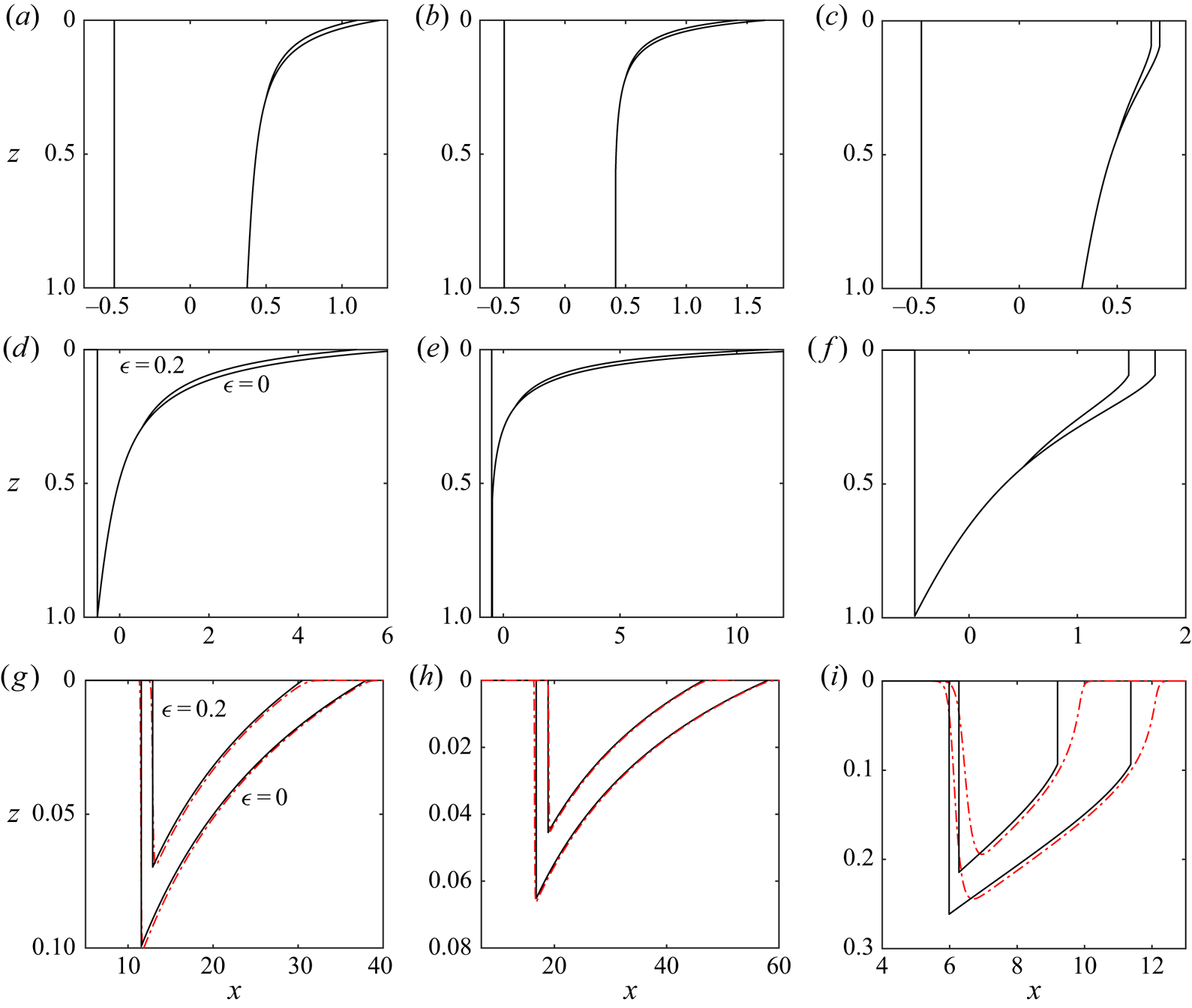
Evolution of the mobile CO $_{2}$. The results from our asymptotic approximations (
 $\mathcal {F}=0$; § 3) are shown as continuous black lines. We include the cases
 $\epsilon =0.2$ and
 $\epsilon =0$. The rows correspond to
 $t=1$,
 $t=t_1$ (the detachment time), and
 $t=50$. The columns corresponds to parameter values of
 $m=0.1$,
 ${\rm \Delta} k=0.5$;
 $m=0.1$,
 ${\rm \Delta} k=-0.3$; and
 $m=0.1$,
 ${\rm \Delta} k=1.6$. The numerical results with
 $\mathcal {F}=0.2$ are plotted as red dot-dashed lines in the bottom row. Note the different axes.
The location of the mobile CO $_{2}$ (black) and the trapped CO
 $_{2}$ (grey) at four times: (a)
 $t=3$, (b)
 $t=7$, (c)
 $t=9$, (d)
 $t=20$. We use a mobility ratio
 $m=0.2$, trapping parameter
 $\epsilon =0.25$ and the permeability decreases towards the bottom of the layer with
 ${\rm \Delta} k =-0.2$. The height,
 $h_0$, at which the flux function,
 $g'(h)$, changes sign is indicated by a blue dot.

At first, the downslope interface advances into the portion of the upslope interface that is receding ( $h>h_0$). At such times, the continuity of the interface at
 $h=\mathcal {H}$ requires that
 \begin{equation} \mathcal{X} = 1/2 + g'(\mathcal{H})t. \end{equation}
We can combine (3.14) and (3.15) to obtain the following equation for the evolution of the shock height:
 \begin{equation} \frac{\mathrm{d} \mathcal{H}}{\mathrm{d} t} = \frac{g(\mathcal{H}) - \mathcal{H} g'(\mathcal{H})}{\mathcal{H} g''(\mathcal{H}) t}. \end{equation}
This equation is separable with implicit solution
 \begin{equation} g(\mathcal{H}) - \mathcal{H} g'(\mathcal{H}) = 1/t, \end{equation}
where the constant of integration is obtained using the initial condition arising from the collision at  $t=t_1$ and is independent of whether or not there is a shock at the top of the layer in the original upslope interface. The downslope interface height,
 $\mathcal {H}(t)$, satisfies (3.17) until it reaches the advancing portion of the interface. We denote this time
 $t=t_2$, given by the solution to
 $\mathcal {H}(t_2)=h_0$. The evolution of
 $\mathcal {H}(t)$ in the time period
 $t_1 < t < t_2$ is independent of
 $\epsilon$ (see figure 8). We substitute
 $\mathcal {H}=h_0$ into (3.17) to obtain the time at which the downslope interface reaches the advancing portion,
 \begin{equation} t_2 = (1+ m^{-1/2})^{2}, \end{equation}
which is independent of  ${\rm \Delta} k$ and
 $\epsilon$.
The evolution of the height of the trailing shock after the detachment from the lower boundary at  $t=t_1$ with
 $m=0.2$. (a) A uniform layer and (b) a layer in which the permeability increases towards the top (
 ${\rm \Delta} k=-1$). In (b) there was a shock at
 $h=1$ in the upslope interface so
 $\mathcal {H}(t_1)<1$.

In the special case that there is no trapping ( $\epsilon =0$), (3.17) provides the downslope interface height at all times and
 $\mathcal {H}$ tends to
 $0$ as
 $t \to \infty$ (provided there is no shock in the upslope interface at the top of the layer).
For  $\epsilon > 0$, the evolution of the travelling shock changes as it enters the advancing portion of the plume (see figure 8). At such times (
 $t>t_2$), the condition for the continuity of the interface at
 $h=\mathcal {H}(t)$ (3.15) is adjusted to
 \begin{equation} \mathcal{X} = 1/2 + (1-\epsilon)g'(\mathcal{H})t. \end{equation}
We combine this with the Rankine–Hugoniot condition (3.14) to obtain the advancing version of (3.16),
 \begin{equation} \frac{\mathrm{d} \mathcal{H}}{\mathrm{d} t} = \frac{g(\mathcal{H}) - (1-\epsilon)\mathcal{H} g'(\mathcal{H})}{\mathcal{H} (1-\epsilon) g''(\mathcal{H}) t}. \end{equation}
This equation is separable but can only be integrated analytically in the special case of equally viscous fluids in a uniform layer (Hesse et al. Reference Hesse, Orr and Tchelepi2008). Instead, we integrate (3.20) numerically. The travelling shock height is then determined for all  $t > t_1$. Beyond the shock (
 $x> \mathcal {X}(t)$), the shape of the interface is given by the upslope solution obtained earlier.
The asymptotic results obtained are shown in figure 6. The top row (figure 6a–c) shows the interfaces at  $t=1$, where each column corresponds to different values of
 $m$ and
 ${\rm \Delta} k$. We use
 $\epsilon =0.2$ and
 $\epsilon =0$. In figure 6(a), there are no shocks in the upslope interface; in figure 6(b), there is a shock at the bottom of the upslope interface whilst in figure 6(c), there is a shock at the top of the upslope interface. The second row shows the interfaces at the time of detachment from the bottom boundary, and the bottom row corresponds to
 $t=50$. The numerical results at
 $t=50$ with
 $\mathcal {F} =0.2$ (red dotted dashed lines) show good agreement with the asymptotic results. This is because the diffusive term in the governing equation becomes negligible for
 $x \gg \mathcal {F}$. In the case that the mobility ratio is small and the permeability is high at the top of the layer (figures 6(g) and 6(h)), the migration distance is large and the agreement is excellent. However, when the permeability is low at the top of the layer, which corresponds to
 ${\rm \Delta} k >0$, the plume migrates less far, and neglecting the diffusive term is a poorer approximation (figure 6i).
For  $\epsilon >0$, there is a time,
 $t_{\infty }$, at which
 $\mathcal {H}(t_{\infty })=0$ and the plume vanishes if there is no shock at the top of the upslope interface. In the case that there is a shock at the top of the upslope interface, the plume vanishes when
 $\mathcal {H}=h_s$. We define the maximum extent that the plume runs upslope as
 \begin{equation} x_{\infty}=1/2+(1-\epsilon)g'(0)t_{\infty} =1/2+(1-\epsilon)k(0)t_{\infty} . \end{equation}
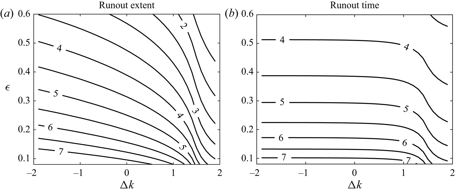
The extent of the plume is larger when the permeability at the top of the layer is high ( ${\rm \Delta} k <0$) because the plume has a longer finger at the top (see figure 9a). The run-out extent may also be interpreted by considering the late-time behaviour. At late times the plume occupies a thin region (
 $h \ll 1$), and the governing equation (2.13) may be approximated by
 \begin{equation} \frac{\partial h}{\partial t} + k(0) \frac{\partial h}{\partial x} = 0. \end{equation}
This suggests that if the early-time and intermediate behaviour when  $h \sim 1$ were ignored then the runout extent would vary linearly with the permeability at the top of the layer,
 $k(0)$. This linear relationship is shown to be a good approximation when the plume runs a long distance (
 $x_{\infty } \gg 1$) in figure 10. Since
 $x_{\infty } \sim k(0) t_{\infty }$ (see (3.21)), the run-out time is approximately independent of the permeability structure when the plume runs a long distance (see figure 9). However, the dimensional final run-out time is inversely proportional to the layer's mean permeability,
 $\bar {K}$, as can be seen through the scaling (2.12). The dimensional run-out distance is independent of the mean permeability. It was shown by Hesse et al. (Reference Hesse, Orr and Tchelepi2008) that the run-out extent also increases with smaller mobility ratios
 $m$.
Contours of (a) the run-out extent of the plume and (b) the time at which all the CO $_{2}$ is trapped for
 $m=0.1$ calculated from our
 $\mathcal {F} \ll 1$ analysis. The labels correspond to
 $\log (x_{\infty })$ and
 $\log (t_{\infty })$, respectively.
Run-out extent ( $x_{\infty }$) in the case
 $m=0.2$ and
 $\epsilon =0.25$ as a function of the permeability contrast,
 ${\rm \Delta} k$. The numerical results (red crosses) in the case
 $\mathcal {F}=0.5$ show excellent agreement with the asymptotic predictions in the case that
 ${\rm \Delta} k \leq 0$. We also include the prediction of linear dependence on
 $k(0)$ (dashed line).

Finally, we note that our run-out predictions are valid even in the case that  $\mathcal {F}$ is not small provided that the plume has spread a long distance (as is the case for
 ${\rm \Delta} k <0$). This is demonstrated by comparing our run-out predictions to the numerical results in the case
 $m=0.2$ and
 $\mathcal {F}=0.5$ in figure 10. The relative error of the asymptotic predictions are 4 % for
 ${\rm \Delta} k=-1$, 5 % for
 ${\rm \Delta} k=0$ and 32 % for
 ${\rm \Delta} k=1$, associated with a much shorter plume for which the neglected diffusive term is relatively important. The run-out distance is increased when the diffusive terms are included in the calculations because the buoyant highly mobile CO
 $_{2}$ finger slumps further upstream owing to the hydrostatic pressure gradients.
3.2. Volume of mobile CO$_{2}$

We apply our results to calculate the volume,  $\nu (t)$, of the mobile CO
 $_{2}$. In the case that there is no trapping (
 $\epsilon =0$), the dimensional volume is always
 $(1-S_a) \phi H_0 L$, which in dimensionless terms is
 $\nu =1$. In the period in which the downslope interface migrates into the receding portion of the plume (
 $0 < t < t_2$), the volume can be calculated from the reduction in the extent of the advancing region associated with trapping at the receding edge,
 \begin{equation} \nu(t) = 1 - \epsilon \int_0^{h_0} g'(z)\,\mathrm{d} z = 1 - \epsilon \left(1 + m^{-1/2} \right)^{-2} t. \end{equation}
At later times ( $t>t_2$), the volume may be obtained from the shock height,
 $\mathcal {H}(t)$,
 \begin{equation} \nu(t) = (1-\epsilon)t [g(\mathcal{H})-\mathcal{H} g'(\mathcal{H})]. \end{equation}
3.3. The relative importance of dissolution of CO$_{2}$

This work has so far neglected any dissolution of the CO $_{2}$ into the ambient brine which might occur (Nordbotten & Celia Reference Nordbotten and Celia2006). Here we incorporate a simple model for dissolution and calculate how it couples with the effects of vertically varying permeability. The dimensionless governing equation (2.13) is adjusted to (MacMinn et al. Reference MacMinn, Szulczewski and Juanes2011; MacMinn & Juanes Reference MacMinn and Juanes2013)
 \begin{equation} \sigma^{-1} \frac{\partial h}{\partial t} + \frac{\partial}{\partial x} [g(h)] = \mathcal{F} \frac{\partial}{\partial x} \left[g(h) \frac{\partial h}{\partial x}\right] - \sigma^{-1} n, \end{equation}
where the loss term is
 \begin{equation} n = \frac{Q_d \mu_r L}{{\rm \Delta} \rho g \bar{K} H_0 \sin \theta} \end{equation}
and  $Q_d$ is the dimensional flux per unit length of the interface associated with dissolution. As an example, in real geological strata the dissolution parameter may be of the order of
 $n \sim 10^{-6}$ (Szulczewski et al. Reference Szulczewski, MacMinn, Herzog and Juanes2012; MacMinn & Juanes Reference MacMinn and Juanes2013). The effect of capillary trapping is adjusted to account for the dissolution term,
 \begin{equation} \sigma=\left\{\begin{array}{@{}ll} 1 & \text{for}\ h_t <-n \\ 1-\epsilon & \text{for}\ h_t >-n. \end{array}\right. \end{equation}
For simplicity, we assume that the CO $_{2}$-saturated brine does not fully flood the layer, which would limit the rate of dissolution (MacMinn et al. Reference MacMinn, Szulczewski and Juanes2011). It is straightforward to adapt our numerical method to incorporate the dissolution term. The final run-out extent obtained from numerical integration of (3.25) is shown in figure 11 as a function of the dimensionless dissolution flux,
 $n$, for particular parameter values. As expected (and studied previously) the extent is reduced with greater dissolution. The extent increases in the case that the permeability increases towards the top boundary. Figure 12 shows the ratio of the run-out distances in a layer in which the permeability increases towards the top with a layer of constant permeability. It was shown earlier that this ratio tends to
 $k(0)$, which is 1.5 in the case that
 ${\rm \Delta} k=-1$, for very large run-out distances. Figure 12 demonstrates that the run-out ratio is insensitive to the dissolution; the run-out ratio varies by just 2.5 % for
 $0 < n < 10^{-4}$. This suggests that although dissolution can have a significant influence on the plume migration, the layer heterogeneity is still key for accurate quantitative modelling. Indeed, the principles we derive in this paper concerning permeability variations carry through to the case in which dissolution is non-negligible.
Final run-out extent,  $x_{\infty }$, as a function of the dissolution parameter,
 $n$, in the case of a uniform layer (
 ${\rm \Delta} k=0$) and a layer with permeability that increases towards the top (
 ${\rm \Delta} k=-1$). The circles denote the predictions without dissolution (
 $n=0$). We use
 $\mathcal {F}=0.5$,
 $\epsilon =0.4$ and
 $m=0.2$.

Ratio of the final run-out distance in a layer with permeability increasing towards the top to the final run-out distance in a layer with constant permeability (cf. figure 11).

3.4. Cross-slope effects
Hitherto we have analysed a two-dimensional model for the post-injection flow of CO $_{2}$. Injection wells are often relatively long in the transverse direction (into the page in figure 2), which motivates a two-dimensional approximation. Presently, we analyse the evolution of a three-dimensional plume to determine the impact of vertically heterogeneous permeability in this case. The transverse coordinate is denoted by
 $Y$ and is scaled with the initial transverse extent,
 $W$ (i.e.
 $y=Y/W$). The initial condition in dimensionless coordinates is given by
 \begin{equation} h=\left\{\begin{array}{@{}ll} 1 & \text{for}\ -1/2 < x < 1/2, -1/2 < y < 1/2\\ 0 & \text{otherwise}. \end{array}\right. \end{equation}
The dimensionless governing equation (2.13) is adjusted to account for cross-slope effects,
 \begin{equation} \sigma^{-1} \frac{\partial h}{\partial t} + \frac{\partial}{\partial x} [ g(h) ] = \mathcal{F} \frac{\partial}{\partial x} \left[g(h) \frac{\partial h}{\partial x}\right] + (\mathcal{F}/w^2) \frac{\partial}{\partial y} \left[g(h) \frac{\partial h}{\partial y}\right], \end{equation}
where  $h=h(x,y,t)$ and
 $w=W/L$ is the aspect ratio of the initial shape. The relative importance of transverse flow depends on the aspect ratio and the inclination of the aquifer through the parameter,
 $\mathcal {F}$. The system is integrated numerically as described in appendix A. Cross-sections of the mobile CO
 $_{2}$ in the
 $x$ direction are shown in figure 13 at
 $t=30$ in the case that
 $\epsilon =0.25$ and
 $\mathcal {F} =0.5$ for an aspect ratio
 $w=5$. There is good agreement between the cross-sections near the centreline and the two-dimensional prediction corresponding to
 $w=\infty$. Away from the centreline, the trailing region of fixed extent advances faster, and eventually this affects the trailing region at the centreline, which in turn shortens the run-out extent.
Cross-sections of the thickness of the mobile CO $_{2}$ in the case that
 $m=0.2$,
 $\epsilon =0.25$,
 ${\rm \Delta} k=0$,
 $\mathcal {F}=0.5$ at
 $t=30$ with aspect ratio
 $w=5$. The shape in the absence of cross-flow effects (
 $w=\infty$) is also included.

Figure 14 shows the runout distance in a layer of constant permeability ( ${\rm \Delta} k=0$) and a layer in which the permeability increases towards the top (
 ${\rm \Delta} k =-1$) as a function of the aspect ratio,
 $w$, for the case
 $\epsilon =0.6$. Although the transverse flow can significantly reduce the extent of the current, its effect is similar for both layers considered. Indeed, the ratio of the run-out distance between the two layers varies by only 4 % with the aspect ratio varying from
 $1 < w < \infty$. Hence, similar to the case of including dissolution, three-dimensional effects can be important but they are also influenced by the heterogeneity.
Run-out distance from the three-dimensional simulation as a function of the aspect ratio,  $w$, for
 $m=0.2$,
 $\epsilon =0.6$, and
 $\mathcal {F}=0.5$ for a layer with constant permeability (
 ${\rm \Delta} k=0$) and a layer with permeability increasing towards the top (
 ${\rm \Delta} k =-1$). The two-dimensional results are indicated by circles.

In the next section, we return to the original model that neglects three-dimensional flow and dissolution. We note that both of these effects act to shorten the extent of the current. Thus, our results from the original model provide conservative estimates of the run-out distances and most importantly demonstrate the impact of vertical permeability variations.
4. Impact of the plume shape at the end of injection
Thus far in this paper we have considered a rectangular release of CO $_{2}$. MacMinn & Juanes (Reference MacMinn and Juanes2009) showed that the distribution of the CO
 $_{2}$ at the end of injection can have a significant influence on run-out length in a uniform horizontal layer. Permeability variations effect the interface evolution in the injection period, which in turn effects the post-injection trapping (Hinton & Woods Reference Hinton and Woods2018). We first describe the behaviour in the injection period. The interface shape during the injection period is complex because it is difficult to determine the proportion of the flux that is partitioned upstream and downstream of the injection point. For simplicity, we assume that the porous layer is sealed far downslope so that all of the injected flux flows upslope. The interface shape in this setting has been calculated in the case of constant permeability (Gunn & Woods Reference Gunn and Woods2011). It was shown that provided the injection period is sufficiently long, the diffusive terms may be neglected and the governing equation is hyperbolic. To obtain the interface shape, we generalise the results of Gunn & Woods (Reference Gunn and Woods2011) to the case of vertically varying permeability by adapting the work of Hinton & Woods (Reference Hinton and Woods2018). During the injection period there is no trapping because
 $\partial h/\partial t \geq 0$ everywhere.
The shape of the interface at the end of injection is controlled by the dimensionless parameter
 \begin{equation} q= \frac{Q \mu_r}{{\rm \Delta} \rho g \bar{K} H_0 \sin \theta}, \end{equation}
where  $Q$ is the injection flux. In the case that
 $q < 1$, the layer does not flood because the injection is slow but for
 $q>1$, the layer floods.
The injection period is  $0 < T < T_i$ and we chose the lengthscale
 $L$ to satisfy
 \begin{equation} (1-S_a) \phi L H_0 = Q T_i, \end{equation}
so that the dimensionless volume of fluid at the end of the injection period is  $\nu =1$. Dimensionless time is still defined from the end of the injection period (
 $t=0$ at
 $T=T_i$). We continue to assume that
 $\mathcal {F} \ll 1$ and neglect the diffusive term in the governing equation (2.13). We note that alternating injection strategies, where brine is injected between periods of CO
 $_{2}$ injection, may enhance the capillary trapping, but such behaviour is beyond the scope of this article (Ide, Jessen & Orr Jr. Reference Ide, Jessen and Orr2007).
4.1. Fast injection (fully-flooded layer, $q \geq 1$)

If the layer fully floods then at the end of the injection period the downslope interface is a shock from  $h=0$ to
 $h=1$ at
 $x=0$. We assume that this downslope interface is a line perpendicular to the boundaries, which is accurate for
 $\mathcal {F} \ll 1$. For a detailed discussion of its structure, see Gunn & Woods (Reference Gunn and Woods2011). The upslope interface shape is given by
 \begin{equation} x= q^{-1} g'(h) + f'(h) \end{equation}
in dimensionless variables, where
 \begin{equation} f(h) = \frac{\psi(h)}{m+(1-m)\psi(h)}, \end{equation}
is the flux function associated with injection. These shapes are shown for some parameter values in figure 15. The initial shape upslope tends towards  $x=f'(h)$ for
 $q \gg 1$.
Interface shape at the end of the injection period for  $m=0.2$ in the cases of (a) uniform layer (
 ${\rm \Delta} k=0$) and (b) layer with permeability that increases towards the top (
 ${\rm \Delta} k=-1$).

The injection term,  $f'(h)$ in (4.3), does not introduce new shocks to the interface provided that (Hinton & Woods Reference Hinton and Woods2018)
 \begin{equation} m < \frac{(2-{\rm \Delta} k)^2}{{\rm \Delta} k^2 - 2 {\rm \Delta} k +4}, \end{equation}
which is the case in most CO $_{2}$ storage projects and we assume this herein. The asymptotic analysis for the post-injection behaviour in the regime
 $\mathcal {F} \ll 1$ is similar to that described in § 3 with a few extra details, which are given in appendix B.
4.2. Slow injection (not fully-flooded, $q < 1$)

In the case that  $q < 1$, the layer is not fully-flooded by the injected fluid (figure 15). The upslope interface has the same shape as (4.3) at the end of injection but only occupies a fraction
 $0 < h < h_i$ of the layer thickness. The downslope interface is at
 $x=0$ and
 $0 \leq h \leq h_i$, and there is an intermediated region where the interface has constant height,
 $h=h_i$ between the upslope and downslope regions (see figure 15). The depth that is flooded
 $h_i$ depends on the injection rate. Mass conservation imposes
 \begin{equation} \psi(h_i) = q. \end{equation}
Since  $\psi (h)$ is an increasing function and
 $\psi (1)=1$, the layer is not fully flooded provided that
 $q < 1$. The asymptotic analysis for the post-injection behaviour in the regime
 $\mathcal {F} \ll 1$ for the case of a layer that is not fully-flooded by CO
 $_{2}$ is given in appendix C.
The run-out distance predicted by the asymptotic analysis is shown as a function of  $q$ in figure 16 with a mobility ratio
 $m=0.2$ and trapping parameter
 $\epsilon =0.3$. The predictions for three permeability structures are shown. With small
 $q$, corresponding to relatively weak injection, the flow during the injection period is strongly influenced by the along-layer component of buoyancy and the end-of-injection plume has a long finger at the top of the layer (see figure 15). This leads to a substantial increase in the run-out distance. At large values of
 $q$, the end-of-injection shape becomes independent of further increases to
 $q$ and the along-layer component of buoyancy is negligible in comparison to the injection pressure. Thus the run-out distance becomes insensitive to further increases to
 $q$.
Run-out extent ( $x_{\infty }$) with a mobility ratio
 $m=0.2$ and
 $\epsilon =0.3$. The initial shape is described in § 4 and is characterised by
 $q$, which quantifies the relative magnitude of the input flux during the injection period.

5. Implications of the results for CO$_{2}$ storage

In the present section, our results are applied to quantify the volume of CO $_{2}$ that can be stored and immobilised via capillary trapping in example geological layers. In particular, we explore the influence of a permeability gradient across the layer and the relative magnitude of the input flux during the injection phase. To assist our analysis, we first define the ‘sweep efficiency’ for a particular layer. The free surface when the plume is immobilised is given by
 $Z=H_R(X)$, which is shown as a shaded region in figure 1; this is the region that is ‘swept’ by the plume. The sweep efficiency is the ratio of the area of the grey region to the area of the red dashed box. This ratio can be calculated by equating the injected volume of CO
 $_{2}$ to the trapped volume of CO
 $_{2}$ (Hesse et al. Reference Hesse, Orr and Tchelepi2008). The injected volume is
 \begin{equation} V=\phi(1-S_a) L H_0, \end{equation}
whilst the final trapped volume is
 \begin{equation} V=\int_0^{L_{\infty}} \phi S_r H_R(X)\,\mathrm{d}X, \end{equation}
where  $L_{\infty }=L x_{\infty }$ is the dimensional run-out distance. This volume represents the trapped CO
 $_{2}$, which does not occupy all the pore space in the grey region in figure 1. The storage efficiency is given by
 \begin{equation} \mathcal{G}=\frac{\int_0^{L_{\infty}} H_R(X)\,\mathrm{d}X}{L_{\infty} H_0} = \frac{1}{\epsilon x_{\infty}}, \end{equation}
where the second equality arises from applying the equations (5.1) and (5.2) for the trapped and injected volumes of CO $_{2}$. The ‘sweep efficiency’ can also be defined as the ratio of the fraction of pore space accessed to the maximum possible fraction in the case of a perfect sweep, which is at most
 $1$.
We first consider how the sweep efficiency,  $\mathcal {G}$, depends on the trapping parameter,
 $\epsilon$, and the permeability gradient,
 ${\rm \Delta} k$. in the idealised case that the initial release of CO
 $_{2}$ takes the form of a rectangle which floods the whole depth of the formation as analysed in § 3. Figure 17 shows the sweep efficiency predicted by our asymptotic results for a mobility ratio of
 $m=0.2$. In the case of a larger capillary trapping fraction,
 $\epsilon$, the plume becomes immobilised more quickly and the finger of CO
 $_{2}$ at the top of the layer progresses a shorter distance. As a result, a greater fraction of the available pore space is accessed. In the case of lower permeability at the top of the layer (
 ${\rm \Delta} k=1$), the finger extent is reduced, which enhances the sweep efficiency. Conversely, the sweep efficiency is lower in the case that the permeability is higher at the top of the layer (
 ${\rm \Delta} k=-1$). We note that with a lower mobility ratio
 $m$, the CO
 $_{2}$ plume has a longer finger at the top of the layer leading to a lower sweep efficiency as has been well-studied by other researchers (Hesse et al. Reference Hesse, Orr and Tchelepi2008; MacMinn & Juanes Reference MacMinn and Juanes2009). As discussed in § 3, the run-out distance,
 $x_{\infty }$ is approximately proportional to the permeability at the top of the layer,
 $k(0)$ for
 ${\rm \Delta} k \leq 0$ and this is illustrated by the black dotted and dashed lines in figure 17. The constants of proportionality,
 $c_1$ and
 $c_2$ are a functions of
 $\epsilon$ and
 $m$.
Sweep efficiency  $1/(\epsilon x_{\infty })$ for
 $m=0.2$ for the case of a rectangular initial release. The efficiency is plotted as a function of
 ${\rm \Delta} k$ for two values of
 $\epsilon$.

We next analyse layers with the same mean permeability and the same permeability at the top of the layer,  $k(0)$, but with different permeability structures, to explore the influence of such heterogeneity. We consider layers with nonlinear permeability structures given by (Hinton & Woods Reference Hinton and Woods2020)
 \begin{equation} k(z) = 1 +\frac{{\rm \Delta} k}{2} \frac{\tanh [(y-1/2)/a]}{\tanh[1/(2a)]}, \end{equation}
which is shown in figure 18(a), and
 \begin{equation} k(z) = 1 -\frac{{\rm \Delta} k}{2} \frac{ \cosh [(y-1/2)/a]-2a \sinh[1/(2a)]}{\cosh[1/(2a)] - 2a \sinh[1/(2a)]}, \end{equation}
which is shown in figure 18(b). These profiles satisfy  $k(0)=1-{\rm \Delta} k/2$ and
 $\int _0^1 k(z)\,\mathrm {d} z=1$. The storage efficiency for these profiles in the case that
 ${\rm \Delta} k=-1$,
 $\epsilon =0.25$ and
 $m=0.2$ is shown in figures 18(c) and 18(d) as a function of the profile parameter
 $a$. The late-time behaviour of each plume, when it occupies a thin region near
 $z=0$, is similar because
 $k(0)$ is fixed. The discrepancy between the storage efficiencies thus depends primarily on the early and intermediate behaviour, which is sensitive to the full permeability structure. This discrepancy and dependence on the permeability structure may be characterised through the height,
 $h_0$, at which the flux function,
 $g'(h)$, changes sign from positive in
 $0 < z < h_0$ to negative in
 $h_0 < z < 1$ (cf. (3.4)). This height,
 $h_0$, is plotted as a function of
 $a$ for the respective permeability profile in figures 18(e) and 18(f). The storage efficiency is inversely related to this height. When
 $h_0$ is small, there is a larger amount of CO
 $_{2}$ trapped in
 $h_0 < z < 1$,
 $-1/2 < x < 1/2$ prior to the plume detaching from the lower boundary (see figure 7) and hence there is less mobile CO
 $_{2}$ that runs upslope so the storage efficiency is greater.
(a,b) Nonlinear permeability profiles given by (5.4) and (5.5) with shape parameter  $a$. (c,d) Corresponding storage efficiencies for these profiles in the case that
 ${\rm \Delta} k=-1$,
 $\epsilon =0.25$ and
 $m=0.2$. (e,f) The height,
 $h_0$ at which the flux function
 $g'(h)$ changes from positive to negative.

We next consider how the sweep efficiency depends on the shape of the plume at the end of the injection phase. We characterise this in terms of the dimensionless injection flux,  $q$ (4.1). In figure 19, the sweep efficiency predicted by our asymptotic results is plotted as a function of the permeability structure (for modest gradients,
 $|{\rm \Delta} k|<1$) for five values of
 $q$. At low values of
 $q$, the layer is not fully flooded by the CO
 $_{2}$ while it is fully flooded for larger values of
 $q$. This leads to a substantial increase in the sweep efficiency. However, ultimately, at sufficiently large values of
 $q$, the efficiency becomes insensitive to
 $q$ because the injection shape is independent of the role of buoyancy. The influence of
 ${\rm \Delta} k$ on the storage efficiency is significant at all values of
 $q$. For comparison, in figure 19, we also include some calculations for the sweep efficiency in the case of a rectangular initial condition as considered in § 3. The rectangular initial shape is more localised than any of the more realistic end-of-injection shapes and the efficiency is correspondingly increased by at least 20 %. The associated predictions of the sweep efficiency are therefore overestimates, and this effect is especially important in the case that
 $q$ is small.
The sweep efficiency,  $1/(\epsilon x_{\infty })$, as a function of the permeability structure,
 ${\rm \Delta} k$, with
 $m=0.2$. The sweep efficiency in the case of the rectangular initial condition of § 3 is included.

The behaviour of the plume and hence the sweep efficiency may be somewhat different in the case that the trapping parameter is very small. Figure 20 shows the run-out distance as a function of  $q$ for a mobility ratio
 $m=0.2$ in a layer with constant permeability (
 ${\rm \Delta} k=0$). The run-out distance in the case of a rectangular release is denoted by a square. When
 $\epsilon =0.25$, there is a similar dependence on
 $q$ to that described above. However, in the case that
 $\epsilon =0.05$, the run-out distance has a very weak dependence on
 $q$ and the plume is predicted to run a very long distance. Over such long distances, the flow behaviour becomes independent of the end-of-injection plume shape and hence changes in
 $q$ have little impact on the sweep efficiency. For higher values of
 $\epsilon$, the CO
 $_{2}$ is trapped faster and thus has a shorter extent, which means that the initial shape has a stronger influence on the run-out extent and sweep efficiency.
The dependence of the sweep efficiency on the initial conditions for three values of the trapping parameter,  $\epsilon$, in a layer with constant permeability (
 ${\rm \Delta} k=0$) and mobility ratio
 $m=0.2$. The initial condition is characterised by the parameter
 $q$, and the squares show the sweep efficiency in the case of a rectangular release.

These results demonstrate the significant uncertainty in the sweep efficiency and hence storage potential for CO $_{2}$ injected into a heterogeneous porous rock. In the case that the trapping fraction is at least
 $0.1$, this uncertainty can be managed in part by increasing the rate of injection provided that the overpressure is not too large to fracture the system. Unfortunately, in the case that
 $\epsilon$ is small, this approach of increasing the injection rate has less effect on the run-out distance. We also note that it may be beneficial to increase the injection pressure above the fracture point because this may improve the injectivity and the storage efficiency. However, fractures may also increase the likelihood of leakage of CO
 $_{2}$. A detailed study of this trade-off is beyond the scope of the present article.
As a quantitative example of these calculations, we consider a laterally extensive layer of rock, into which we inject from a long horizontal well of length 5 km. The layer has porosity  $\phi =0.2$, inclination gradient
 $\tan \theta =0.02$ and thickness
 $H_0=10\ \textrm {m}$. We assume that the CO
 $_{2}$ runs updip and estimate the storage potential and the distance run-out by the CO
 $_{2}$ when it is all capillary trapped. We take typical parameter values of
 $m=0.2$ and
 $S_R=0.35$,
 $S_a=0.3$, which yields
 $\epsilon =0.5$ (Bachu & Bennion Reference Bachu and Bennion2008). We suppose that CO
 $_{2}$ is injected for 10 years at a rate of 0.5 Mt per year distributed across the 5 km well. With density
 $\rho =750\ \textrm {kg}\ \textrm {m}^{-3}$, the total volume of CO
 $_{2}$ injected is
 $6.7 \times 10^6\ \textrm {m}^3$, which corresponds to a characteristic end-of-injection length of
 $L=1\ \textrm {km}$ (see (5.1)). The transverse length is thus much greater than the lateral end-of-injection length and so the ensuing motion can be approximated as two-dimensional (see § 3.4). The flux per unit length of well during the injection period is
 $Q =4 \times 10^{-6}\ \textrm {m}^2\ \textrm {s}^{-1}$. The importance of buoyancy is quantified by the parameter
 \begin{equation} \mathcal{F} = \frac{H_0}{L \tan \theta} = 0.5. \end{equation}
Although this is not small, the run-out predictions from our  $\mathcal {F}=0$ analysis show good agreement with the numerical results with
 $\mathcal {F}=0.5$ for
 ${\rm \Delta} k \leq 0$ and
 $m=0.2$, so the plume becomes long and thin and the role of buoyancy is important only at early times (see figure 10). We take the upslope buoyancy velocity to be
 \begin{equation} U_B = \frac{{\rm \Delta} \rho g \bar{K} \sin \theta}{\mu_r} = 10^{-6}\ \textrm{m}\ \textrm{s}^{-1} \end{equation}
and then  $q=Q/(U_B H_0)=0.4$. From these parameters, we calculate that the run-out distance is 33 kilometres in a uniform layer and 47 kilometres in a layer in which the permeability increases linearly towards the top with
 ${\rm \Delta} k=-1$. The sweep efficiencies in the two layers are
 $\mathcal {G}=5.3\,\%$ and
 $\mathcal {G}=4.2\,\%$, respectively. We calculate that the dimensional time for the CO
 $_{2}$ to be entirely trapped is approximately 60 years in either case.
6. Conclusion
We have investigated the capillary trapping of CO $_{2}$ in an inclined layer of porous rock in which the permeability varies with depth. CO
 $_{2}$ is left behind in the pore throats as the trailing edge of the CO
 $_{2}$ plume is displaced by the ambient brine while the leading edge of the CO
 $_{2}$ migrates upslope. Eventually the trailing edge catches up with the leading edge and all the CO
 $_{2}$ becomes immobilised. In the case that the CO
 $_{2}$ migrates a long distance relative to its initial length, we have shown that the run-out distance is approximately linearly proportional to the permeability at the top of the layer because the mobile CO
 $_{2}$ predominantly occupies a region near this upper boundary. The permeability profile away from the upper boundary influences the early and intermediate behaviour and this has a smaller but important effect on the run-out distance and hence the fraction of pore space that may be accessed by the CO
 $_{2}$. The time taken for the CO
 $_{2}$ to become entirely immobilised is somewhat insensitive to the permeability structure given the same mean permeability. We have shown that these principles concerning the impact of heterogeneous permeability carry over to a three-dimensional geometry, where the plume has a finite transverse extent, and to the case in which dissolution is important.
We have also considered the influence of the distribution of the CO $_{2}$ at the end of the injection period. Generally, increasing the injection rate leads to a deeper and more localised injection plume, and this reduces the run-out distance. At high rates of injection, the plume shape during injection, and hence the post-injection trapping, becomes independent of increases to the input flux. The run-out distance is then predominantly controlled by the permeability structure of the rock.
Our results have significant implications for the assessment of the storage potential of CO $_{2}$ storage sites and of the optimal rate at which to inject the CO
 $_{2}$. The economic viability and security of a storage site depends critically on the volume of CO
 $_{2}$ that can be stored there. The volume stored can be significantly increased by injecting at a higher rate, but eventually further increases in the injection rate do not change the storage volume. Moreover, the injection rate may be limited by the fracture strength of the formation, especially in lower permeability formations.
Acknowledgements
The authors wish to thank T. Espie for his support of this work, and BP and EPSRC for the award of a CASE studentship funding the research.
Declaration of interests
The authors report no conflict of interest.
Appendix A. Numerical method
The two-dimensional governing equation (2.13) is integrated numerically, using the finite-difference method of Kurganov & Tadmor (Reference Kurganov and Tadmor2000). The system is solved on a fixed domain  $(-a_1,a_2) \times (0,t_{{end}})$, where
 $a_1$ and
 $a_2$ are chosen to exceed the greatest extent of the plume in the time interval
 $(0,t_{{end}})$. The boundary conditions at the ends of the interval are
 $h=0$ and the initial condition at
 $t=0$ is given in each section of the paper. The diffusive and advective fluxes in (2.13) are approximated by a second-order central discretisation in the spatial coordinate. A minmod flux limiter (see § 2 of Kurganov & Tadmor Reference Kurganov and Tadmor2000) is used to accurately resolve the regions of fixed extent where the interface has a large gradient. The time-stepping is achieved using a second-order Runge–Kutta method. The numerical method is extended to consider diffusive fluxes in two spatial dimensions following § 4.3 of Kurganov & Tadmor (Reference Kurganov and Tadmor2000).
Appendix B. Asymptotic analysis in the case of relatively fast injection ($q \geq 1$)

We outline the asymptotic behaviour for the post-injection migration of CO $_{2}$ in the regime
 $\mathcal {F} \ll 1$ for the end-of-injection shape described in § 4.1 corresponding to sufficiently fast injection that the layer is fully flooded by CO
 $_{2}$ (
 $q \geq 1$). After the end of injection, the interface evolves in a similar manner to that described in § 3, with shape given by
 \begin{equation} x=\left\{\begin{array}{@{}ll} f'(h) + \big[q^{-1}+(1-\epsilon) t \big] g'(h) & \text{for}\ 0 < h < h_0,\\ f'(h) + \big[q^{-1}+ t \big] g'(h) & \text{for}\ h_0 < h < 1, \end{array}\right. \end{equation}
where we have neglected diffusive terms as before. Provided the condition (4.5) is met, there are two possibilities for the evolution of the upslope interface post-injection: (i) no shocks develop until the interaction with the downslope interface or (ii) a shock develops at the bottom of the layer as described in § 3. The case of a shock at the top is not possible given the requirement (4.5). For case (i), the interaction with the downslope interface ( $x=0$) occurs at a time
 \begin{equation} t_1=1-q^{-1}. \end{equation}
Subsequently the downslope interface begins to move. Whilst the downslope interface advances into the receding portion of the upslope interface ( ${\mathcal {H} > h_s}$), its position [
 $x=\chi (t)$] and height [
 $h=\mathcal {H}(t)$] evolves according to
 \begin{equation} \chi = f'(\mathcal{H}) + (q^{-1}+ t) g'(\mathcal{H}), \quad \frac{\mathrm{d} \mathcal{H}}{\mathrm{d} t} = \frac{g(\mathcal{H})/\mathcal{H} - g'(\mathcal{H})}{(q^{-1}+ t) g''(\mathcal{H}) + f''(\mathcal{H})}. \end{equation}
We numerically integrate to obtain  $\mathcal {H}(t)$ and
 $\chi (t)$. The system changes, at time
 $t=t_2$, when the trailing downslope interface migrates into the advancing portion of the upslope interface [i.e.
 $\mathcal {H}(t_2) = h_0$],
 \begin{align} \chi = f'(\mathcal{H}) + \big[q^{-1}+(1-\epsilon) t \big] g'(\mathcal{H}),\quad \frac{\mathrm{d} \mathcal{H}}{\mathrm{d} t} = \frac{g(\mathcal{H})/\mathcal{H} - (1-\epsilon) g'(\mathcal{H})}{[q^{-1}+(1-\epsilon) t ] g''(\mathcal{H}) + f''(\mathcal{H})}. \end{align}
We integrate this equation and obtain the run-out time and distance in the case  $\epsilon >0$, which occur when the CO
 $_{2}$ has been entirely trapped (
 $\mathcal {H}=0$).
In case (ii), the upslope interface develops a shock at  $h=1$ at a time
 \begin{equation} t_s = -f''(1)/g''(1) -q^{-1}. \end{equation}
With a linearly varying permeability, this time can be rewritten as
 \begin{equation} t_s = 1 -q^{-1} + \frac{2m (1+{\rm \Delta} k/2)^2}{g''(1)} > 1-q^{-1} (= t_1), \end{equation}
because  $g''(1) >0$ is the condition required for a shock to develop in the upslope interface at
 $h=1$. The bottom of the upslope interface therefore interacts with the downslope interface prior to a shock in the upslope interface occurring. The subsequent evolution of the downslope shock is as in case (i) described above.
Appendix C. Asymptotic analysis in the case of relatively slow injection ($q \leq 1$)

We outline the asymptotic behaviour for the post-injection migration of CO $_{2}$ in the regime
 $\mathcal {F} \ll 1$ for the end-of-injection shape described in § 4.2 corresponding to sufficiently slow injection that the layer is not fully flooded by CO
 $_{2}$ (
 $q \leq 1$). Immediately after the end of injection, the downslope shock steadily moves into the constant thickness region of the plume with position given by
 \begin{equation} \chi = g(h_i)t/h_i. \end{equation}
The shock eventually reaches the upslope interface. In the case that  $h_i < h_0$ [corresponding to
 $q<(1+m^{-1/2})^{-1}$], the upslope interface is nowhere receding and its trailing edge has position
 \begin{equation} x= f'(h_i) + \big[q^{-1}+(1-\epsilon) t \big] g'(h_i) \end{equation}
and the interaction occurs at time
 \begin{equation} t_1 = \frac{f'(h_i) + q^{-1}g'(h_i)}{g(h_i)/h_i - (1-\epsilon)g'(h_i)}. \end{equation}
The shock height subsequently evolves according to (B 4). In the case that  $h_i > h_0$, the trailing edge of the upslope interface is receding and the interaction with the downslope interface occurs at a time
 \begin{equation} t_1 = \frac{f'(h_i) + q^{-1}g'(h_i)}{g(h_i)/h_i - g'(h_i)}. \end{equation}
The evolution of the downslope shock then evolves according to (B 3) until  $\mathcal {H}=h_0$ and then its height evolves according to (B 4).


 Open access

