2 Forced Korteweg–de Vries equation

The asymptotic derivation of the fKdV equation for internal waves was first given by Grimshaw & Smyth (Reference Grimshaw and Smyth1986) and Melville & Helfrich (Reference Melville and Helfrich1987), and its relevant solutions can be found there, and in many other works. For a recent review see Grimshaw (Reference Grimshaw2010). The outcome is briefly summarised here. At the leading order we get linear long wave theory,

where $\unicode[STIX]{x1D701}$ is the vertical particle displacement relative to the basic state, defined by the background density field $\unicode[STIX]{x1D70C}_{0}(z)$ and background current $u_{0}(z)$ . The modal function $\unicode[STIX]{x1D719}(z)$ satisfies the system

In general this has an infinite set of solutions for $\unicode[STIX]{x1D719}(z)$ and the linear long wave speed $c$ , but for oceanic internal waves it is customary to examine only mode one which has the fastest internal wave speed (formally the lowest mode zero is the surface wave mode with speed $c\approx (gh)^{1/2}$ in the absence of background current). As usual we normalise $\unicode[STIX]{x1D719}$ so that $\unicode[STIX]{x1D719}(z_{m})=1$ where $z=z_{m}$ is the location of the extremum of $\unicode[STIX]{x1D719}$ . Then the fKdV equation, written in the reference frame of the topography, given by $z=-h+b(x)$ , is

At resonance (that is, at criticality, see below in the next paragraph), $c=\unicode[STIX]{x1D6E5}\approx 0$ and this reduces to the more familiar form

Here the modal function $\unicode[STIX]{x1D719}$ is evaluated at $c=0$ , but $c=\unicode[STIX]{x1D6E5}$ is retained in the leading-order terms to ensure that all terms remain in balance.

It is now useful to consider the special case when $u_{0}=U=\text{const}$ . Then the speed $c=U-c_{0}$ where $c_{0}$ is the intrinsic linear long wave speed, that is the speed in the absence of a background flow. In that case $c=c_{0}(F-1)$ where $F=U/c_{0}$ is the Froude number, and the modal equation becomes

The coefficients become, to leading order,

When $U$ varies temporally, the coefficients $\unicode[STIX]{x1D707}_{0},\unicode[STIX]{x1D6FF}_{0}$ remain constant, and in the fKdV equation (2.4), only the coefficients $c=U-c_{0}=c_{0}(F-1)$ and $\unicode[STIX]{x1D6FE}_{0}$ vary, where

Next, rescale by

so that (2.6) adopts the non-dimensional canonical form, after removing the tilde superscript,

For mode one, since $\unicode[STIX]{x1D719}$ has a positive extremum, $\unicode[STIX]{x1D70E}_{0}>0$ and so the forcing is positive when $\unicode[STIX]{x1D707}_{0}b>0$ but negative when $\unicode[STIX]{x1D707}_{0}b<0$ . In particular, flow of a two-layer fluid with a near-surface pycnocline over a sill is equivalent to negative forcing.

The solutions fall into three categories (see Grimshaw & Smyth Reference Grimshaw and Smyth1986 and Grimshaw Reference Grimshaw2010): subcritical $\unicode[STIX]{x1D6E5}<\unicode[STIX]{x1D6E5}_{m}<0$ , transcritical $\unicode[STIX]{x1D6E5}_{m}<\unicode[STIX]{x1D6E5}<\unicode[STIX]{x1D6E5}_{M}$ and supercritical $\unicode[STIX]{x1D6E5}>\unicode[STIX]{x1D6E5}_{M}>0$ . Here the regime boundaries $\unicode[STIX]{x1D6E5}_{m,M}$ depend on the forcing. For the asymptotic limit of broad forcing, also known as the hydraulic limit,

where $b_{M}$ is the maximum obstacle displacement and is positive when $b>0$ , or negative when $b<0$ . In the usual fKdV limit, we can set $F\approx 1$ here, but using the relation $F=1+\unicode[STIX]{x1D6E5}$ a refinement is

Thus the supercritical boundary is increased and the subcritical boundary is decreased.

The subcritical and supercritical regimes are essentially linear and near the obstacle in a steady state. They are given by the approximate expressions valid for large $|\unicode[STIX]{x1D6E5}|$ and as $t\rightarrow \infty$ ,

Here $H(x)$ is the Heaviside function. The subcritical solution (2.16) is obtained by solving the steady-state linearised form of the fKdV equation (2.13), while for the supercritical solution (2.17) the exponential decay away from the localised forcing is omitted as this occurs on a very short length scale $\unicode[STIX]{x1D6E5}^{-1/2}$ . Note that in (2.16) $\unicode[STIX]{x1D6E5}=F-1$ is bounded from below by $F=0$ . 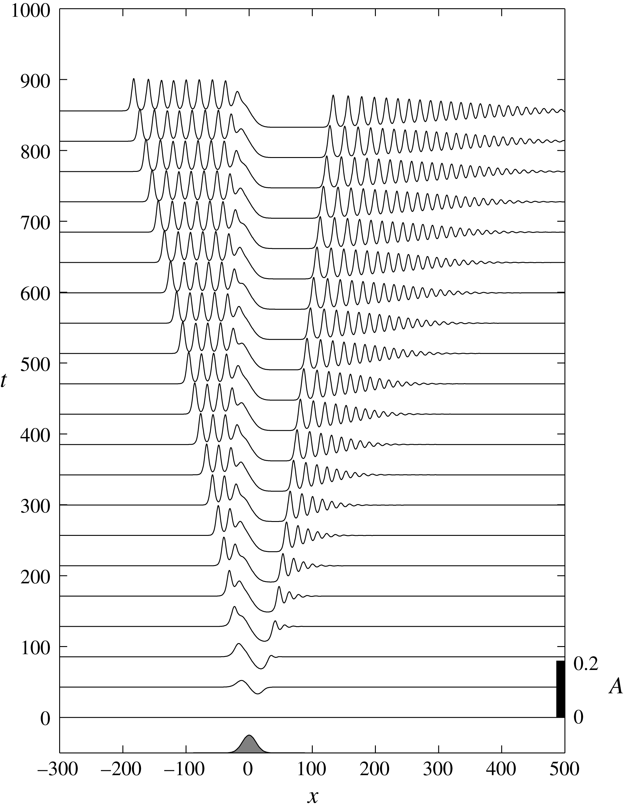Close to the regime boundaries, the nonlinear terms provide corrections, and in particular the sinusoidal lee waves in (2.16) are replaced with cnoidal waves. In the transcritical regime, for positive forcing, the solution consists of a steady hydraulic solution over the obstacle, terminating with an upstream elevation resolved by an upstream propagating undular bore, and a downstream depression terminated by a downstream propagating undular bore. Figure 1 shows a numerical solution of (2.13) with $b_{M}=0.01$ and $\unicode[STIX]{x1D6E5}=0$ . The constant forcing is started impulsively with $A(x,0)=0$ . Details of the numerical scheme are discussed below. 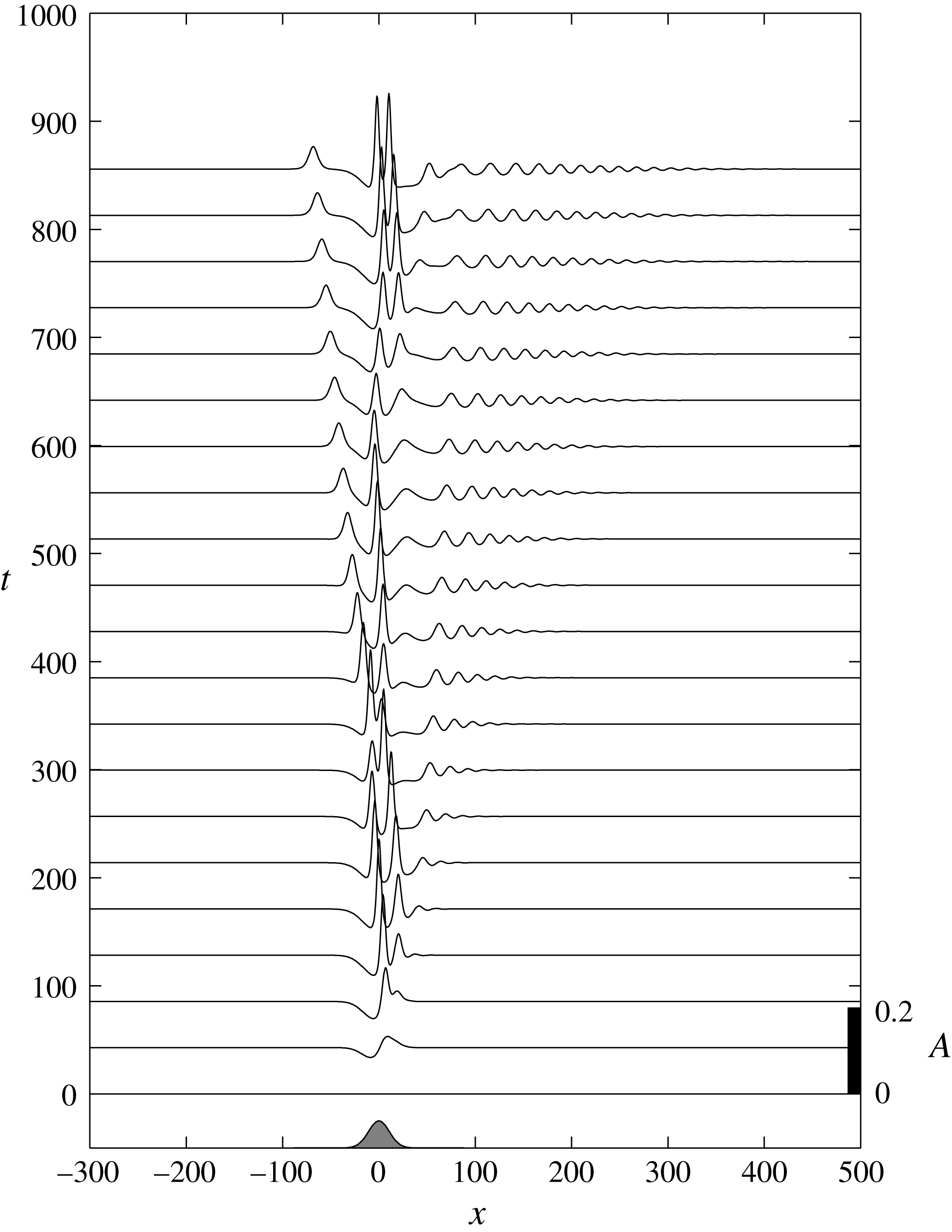As $\unicode[STIX]{x1D6E5}$ increases towards $\unicode[STIX]{x1D6E5}_{M}$ the upstream undular bore resembles more a sequence of solitary waves, and the downstream undular bore weakens, and as $\unicode[STIX]{x1D6E5}$ decreases towards $\unicode[STIX]{x1D6E5}_{m}$ the upstream undular bore weakens, and the downstream undular bore intensifies. For negative forcing, the same scenario occurs upstream and downstream, but the flow over the obstacle remains unsteady, and there is some modulation of the upstream and downstream undular bores as illustrated in figure 2 for $b_{M}=-0.01$ and constant $\unicode[STIX]{x1D6E5}=0$ .

Figure 1.

Numerical solution of the fKdV equation (2.13) for a localised obstacle, with $b_{M}=0.01$ and $\unicode[STIX]{x1D6E5}=0$ . The location and shape of the topography (arbitrary amplitude) is shown at the bottom of the plot.

Figure 2.

The same as figure 1 but now for $b_{M}=-0.01$ .

3 Generation of internal undular bores by tidal interaction with symmetric topography

The generation of internal undular bores by tidal flow can now be modelled by supposing that $\unicode[STIX]{x1D6E5}$ varies slowly with time. Suppose for instance that $\unicode[STIX]{x1D6E5}$ increases from a large negative value (formally $\unicode[STIX]{x1D6E5}=-1$ where $F=0$ ) to a maximum value of $\unicode[STIX]{x1D6E5}_{max}$ and then decreases back again, modelling the onset of an increasing tidal current followed by a decreasing tidal current, both in the same positive $x$ -direction. Then three scenarios can be identified.

1. (i) If $\unicode[STIX]{x1D6E5}_{max}<\unicode[STIX]{x1D6E5}_{m}$ then the flow is always subcritical. On the increasing tide lee waves are generated, which reach a maximum amplitude at $\unicode[STIX]{x1D6E5}_{max}$ . These waves cannot be maintained as $\unicode[STIX]{x1D6E5}$ decreases on the decreasing tide, and so propagate over the obstacle and then upstream.

2. (ii) If $\unicode[STIX]{x1D6E5}_{m}<\unicode[STIX]{x1D6E5}_{max}<\unicode[STIX]{x1D6E5}_{M}$ the flow reaches criticality at its peak. During the peak period, internal undular bores propagate slowly both upstream and downstream. But as the tide recedes, the upstream and downstream undular bores propagate back upstream. This could be identified as the Maxworthy mechanism (Maxworthy Reference Maxworthy1979). In his laboratory experiment a large depression formed in the lee of the obstacle when the tidal flow reached criticality. As the tidal flow slackened the depression moved back upstream and evolved into several internal solitary waves.

3. (iii) If $\unicode[STIX]{x1D6E5}_{max}>\unicode[STIX]{x1D6E5}_{M}$ the flow passes through the transcritical regime as the tide develops, passes into the supercritical regime at the peak tide, and then again passes through the transcritical regime as it weakens. In this case the strongest internal undular bores are generated in the middle stage as the tide strengthens and then again at the middle stage as the tide weakens. On the growing tide these undular bores are swept downstream as the peak tide is approached, but propagate back upstream as the tide weakens.

We next present some numerical solutions for time-dependent forcing $F(t)$ . We consider the specific case of sinusoidal barotropic tidal flow

over half of a tidal cycle, $0\leqslant t\leqslant \unicode[STIX]{x03C0}/\unicode[STIX]{x1D714}$ , where $\unicode[STIX]{x1D714}$ is the tidal frequency. 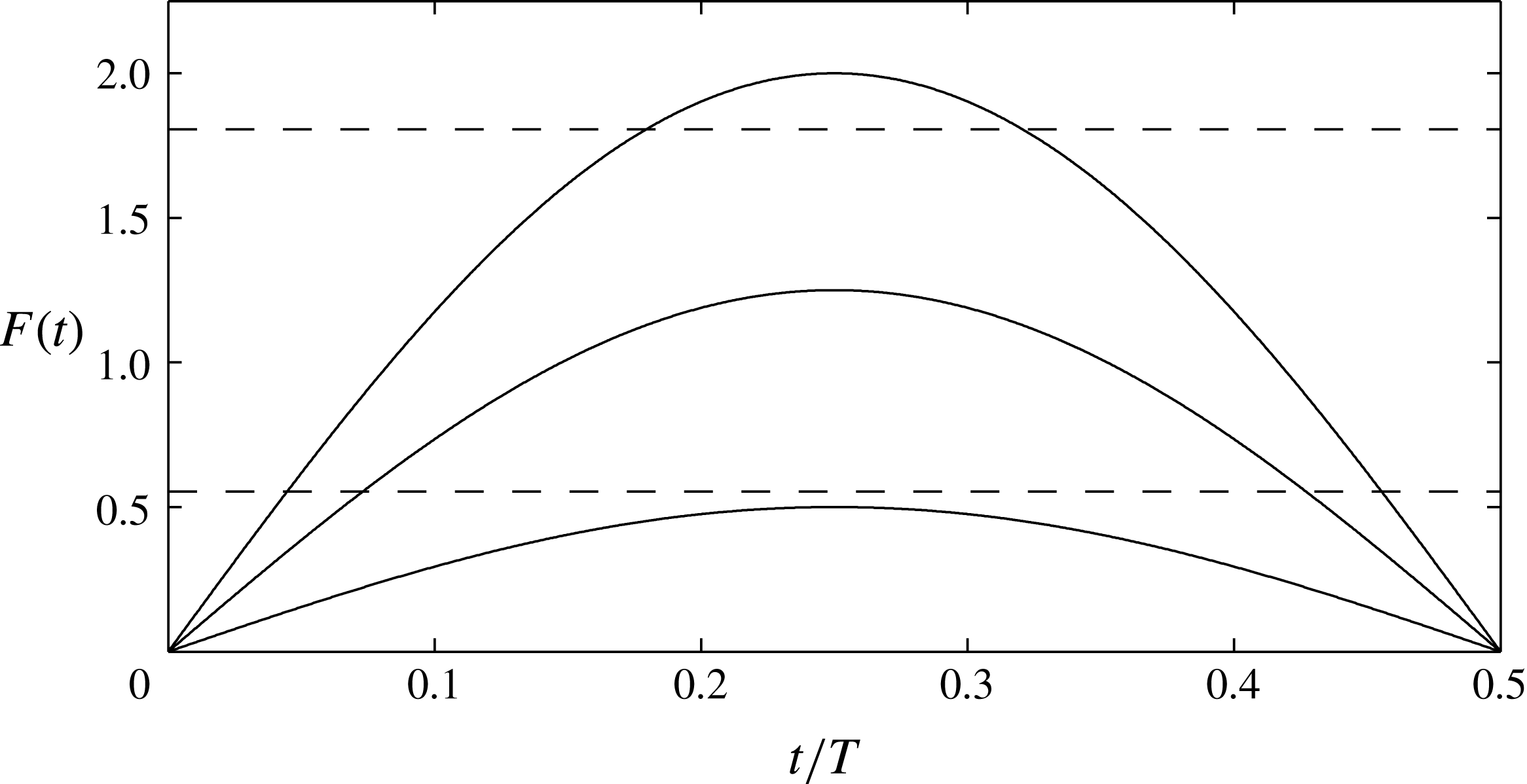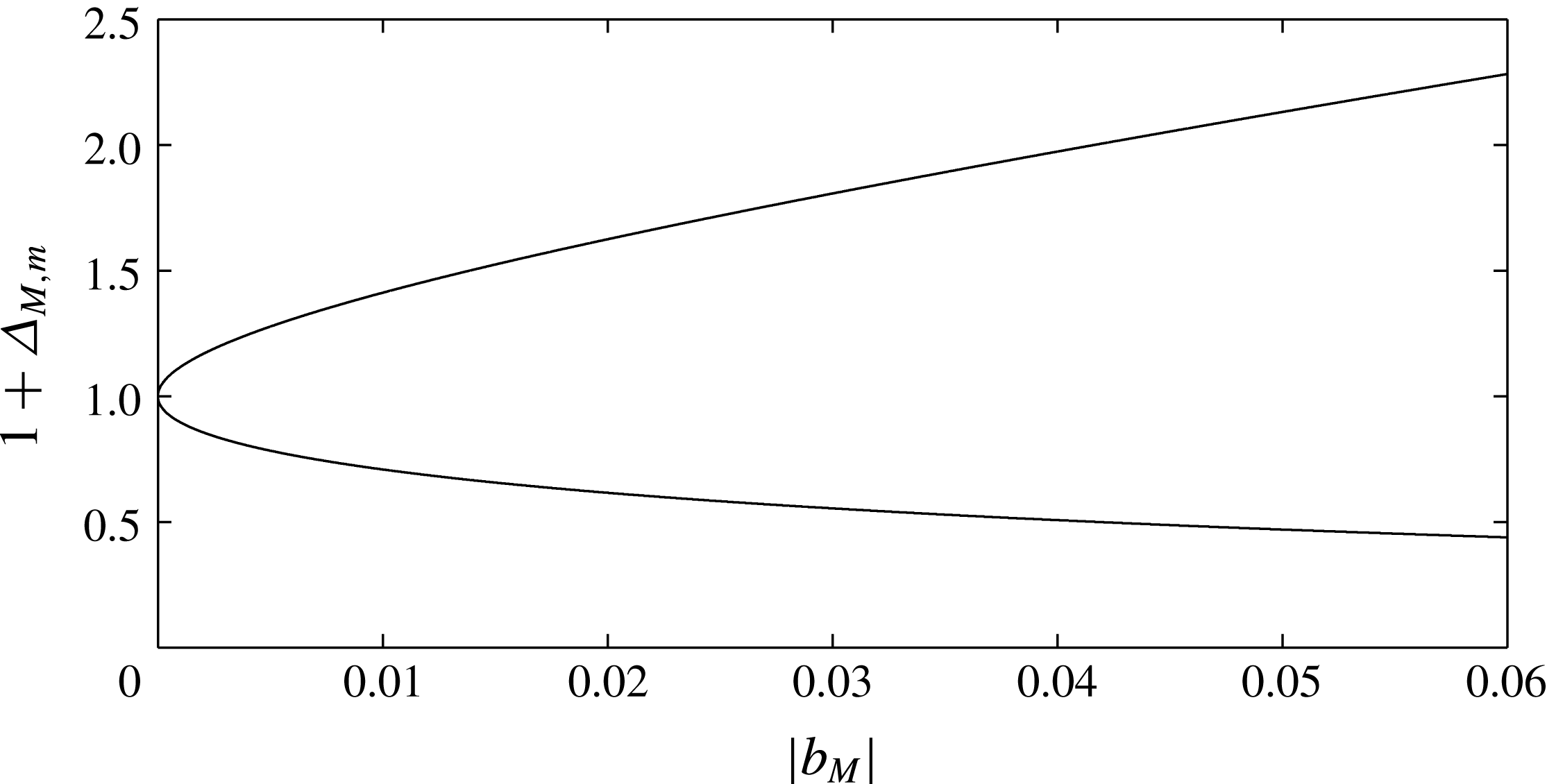This forcing may pass through the resonant regime on both the acceleration and deceleration phase, may reside in the resonant regime for an extended period, or may not be large enough to enter the resonant regime, depending on $\unicode[STIX]{x1D6E5}_{max}=F_{max}-1$ and $\unicode[STIX]{x1D6E5}_{M,m}$ from (2.15) (or (2.14)). Figures 3 and 4 show, respectively, an example of these three possibilities for $b_{M}=0.03$ and the resonant band $1+\unicode[STIX]{x1D6E5}_{M,m}$ from (2.15).

Figure 3.

$F(t)$ from (3.1) for $F_{max}=0.5$ , $1.25$ and $2$ . Here $T=2\unicode[STIX]{x03C0}/\unicode[STIX]{x1D714}$ . The dashed lines indicate the resonant regime from (2.15) for $|b_{M}|=0.03$ .

Figure 4.

The resonant band limits $1+\unicode[STIX]{x1D6E5}_{M,m}$ from (2.15).

Using (2.12) the scaled frequency $\tilde{\unicode[STIX]{x1D714}}=\unicode[STIX]{x1D714}(\unicode[STIX]{x1D6FF}/c_{0}^{3})^{1/2}$ (re-introducing the tildes). With the (dimensional) topography

where $s(x)$ is a shape function with $\max (s)=1$ and $b_{M}$ is the amplitude, the forcing term in (2.13) becomes

Estimates for the non-dimensional parameters $\tilde{\unicode[STIX]{x1D714}}$ and $\tilde{b}_{M}$ are found by considering a Boussinesq, two-layered stratification with layer depths $h_{i}$ and densities $\unicode[STIX]{x1D70C}_{i}$ in each layer. Here $i=1,2$ indicates the upper and lower layers, respectively. The coefficients (2.10) and (2.11) become

with $g^{\prime }=g(\unicode[STIX]{x1D70C}_{2}-\unicode[STIX]{x1D70C}_{1})/\unicode[STIX]{x1D70C}_{1}.$ Conditions representative of the coastal ocean are total depth $H=h_{1}+h_{2}=100{-}300~\text{ m}$ , $0.1<h_{1}/H<0.5$ , $|b_{M}|/H\lesssim 0.2$ , $g^{\prime }=0.01{-}0.02~\text{m}~\text{s}^{-2}$ and semi-diurnal tidal frequency $\unicode[STIX]{x1D714}=1.41\times 10^{-4}~\text{s}^{-1}$ . From (2.12), the normalising length scale $(\unicode[STIX]{x1D6FF}_{0}/c_{0})^{1/2}=10{-}60~\text{m}$ and time scale $(\unicode[STIX]{x1D6FF}_{0}/c_{0}^{3})^{1/2}=30{-}70~\text{s}$ . These parameter ranges give $|\tilde{b}_{M}|\lesssim 0.05$ and $\tilde{T}=2\unicode[STIX]{x03C0}/\tilde{\unicode[STIX]{x1D714}}=700{-}1500$ . The topographic shape is taken to be a Gaussian,

with scaled width $\tilde{w}_{b}=w_{b}(c_{0}/\unicode[STIX]{x1D6FF}_{0})^{1/2}=25{-}100$ for $w_{b}/H\approx 5{-}10$ .

Numerical solutions of (2.13) were obtained with a Fourier pseudo-spectral discretisation in $x$ . The nonlinear term was dealiased using the 2/3-rule truncation. Temporal integration employed a third-order, low-storage Runge–Kutta scheme (Williamson Reference Williamson1980). The barotropic forcing was given by (3.1) for $t\leqslant T/2$ and the topographic shape by (3.5). The maximum forcing $F_{max}=0.5{-}2$ , $T=600{-}1400$ , $|b_{M}|\leqslant 0.06$ and $w_{b}=25$ and $75$ (after again dropping the tildes). The scheme is periodic in $x$ , although the domain size was always taken large enough to avoid end effects. A typical domain had a length of $1500$ and used $3072$ or $4096$ grid cells. A typical time step was $0.001$ .

Figure 5.

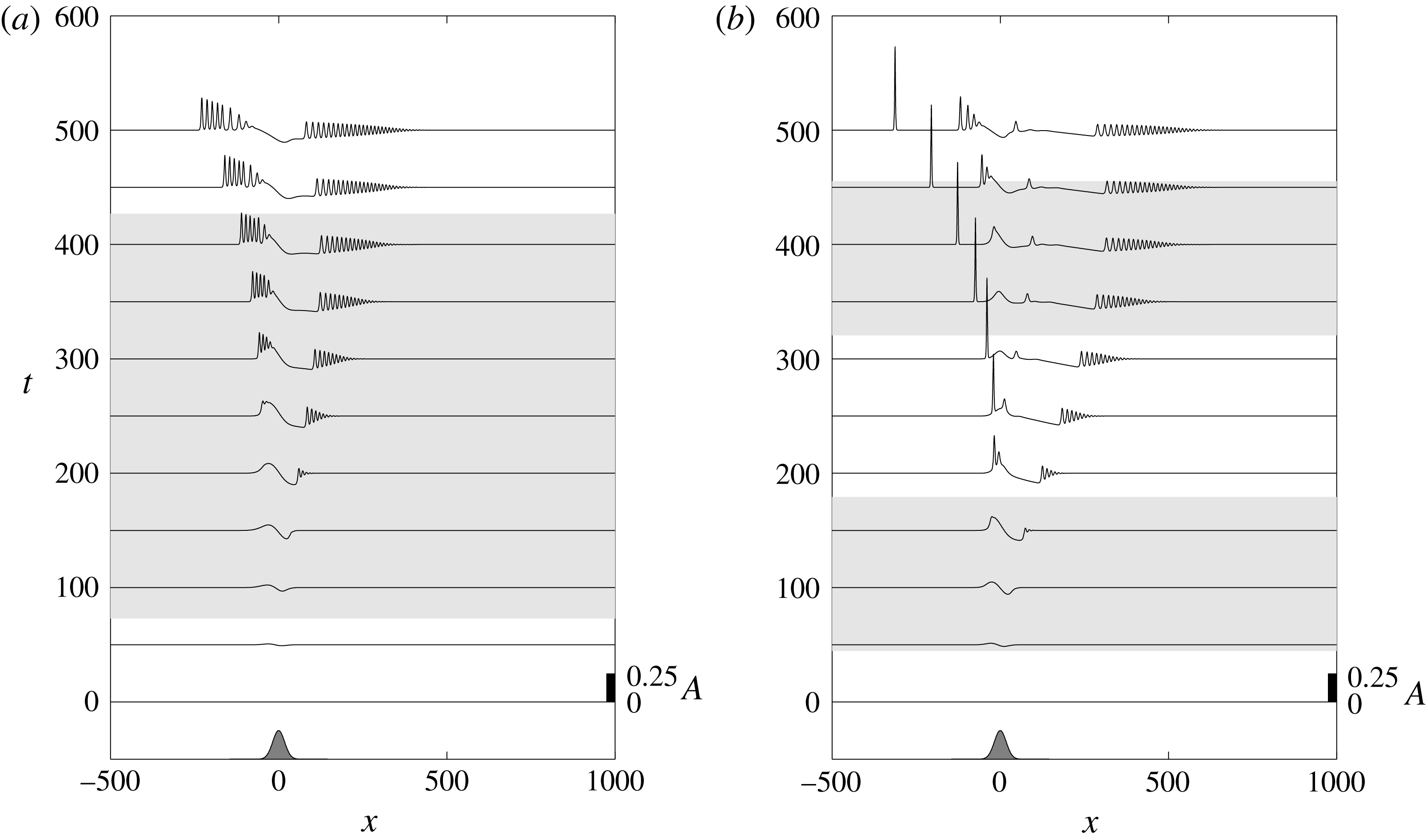
(a) Solution of (2.13) for $(b_{M},T,w_{b})=(0.03,1000,25)$ with $F_{max}=1.25$ . (b) The same but now $F_{max}=2$ . The location and shape of the topography (arbitrary amplitude) is shown at the bottom of the plot. The light grey shading indicates the time when the forcing is in the critical region, $\unicode[STIX]{x1D6E5}_{m}<F(t)-1<\unicode[STIX]{x1D6E5}_{M}$ , from (2.15) and (3.1).

Figure 5(a) shows the solution $A(x,t)$ for a run with $F_{max}=1.25$ , $T=1000$ , $w_{b}=25$ and positive forcing $b_{M}=0.03$ . Here $\unicode[STIX]{x1D6E5}_{m}<\unicode[STIX]{x1D6E5}_{max}<\unicode[STIX]{x1D6E5}_{M}$ from figure 3. The passage of the forcing through the resonance regime excites undular bores upstream and downstream of the topography (centred at $x=0$ ) similar to the constant $\unicode[STIX]{x1D6E5}$ example in figure 1. However the upstream waves are less regularly separated, reflecting the time variation of $\unicode[STIX]{x1D6E5}$ , and after the forcing peaks (at $t=250$ ) the downstream bore begins to move upstream (scenario 2 above). Figure 5(b) shows the evolution for $F_{max}=2$ . Here $\unicode[STIX]{x1D6E5}_{max}>\unicode[STIX]{x1D6E5}_{M}$ (scenario 3) so the forcing involves distinct acceleration and deceleration passages through the resonant region. This gives rise to a single upstream propagating solitary wave generated on the accelerating phase. A trailing packet evolves on the deceleration phase of the forcing from the release of the supercritical-like response over the topography.

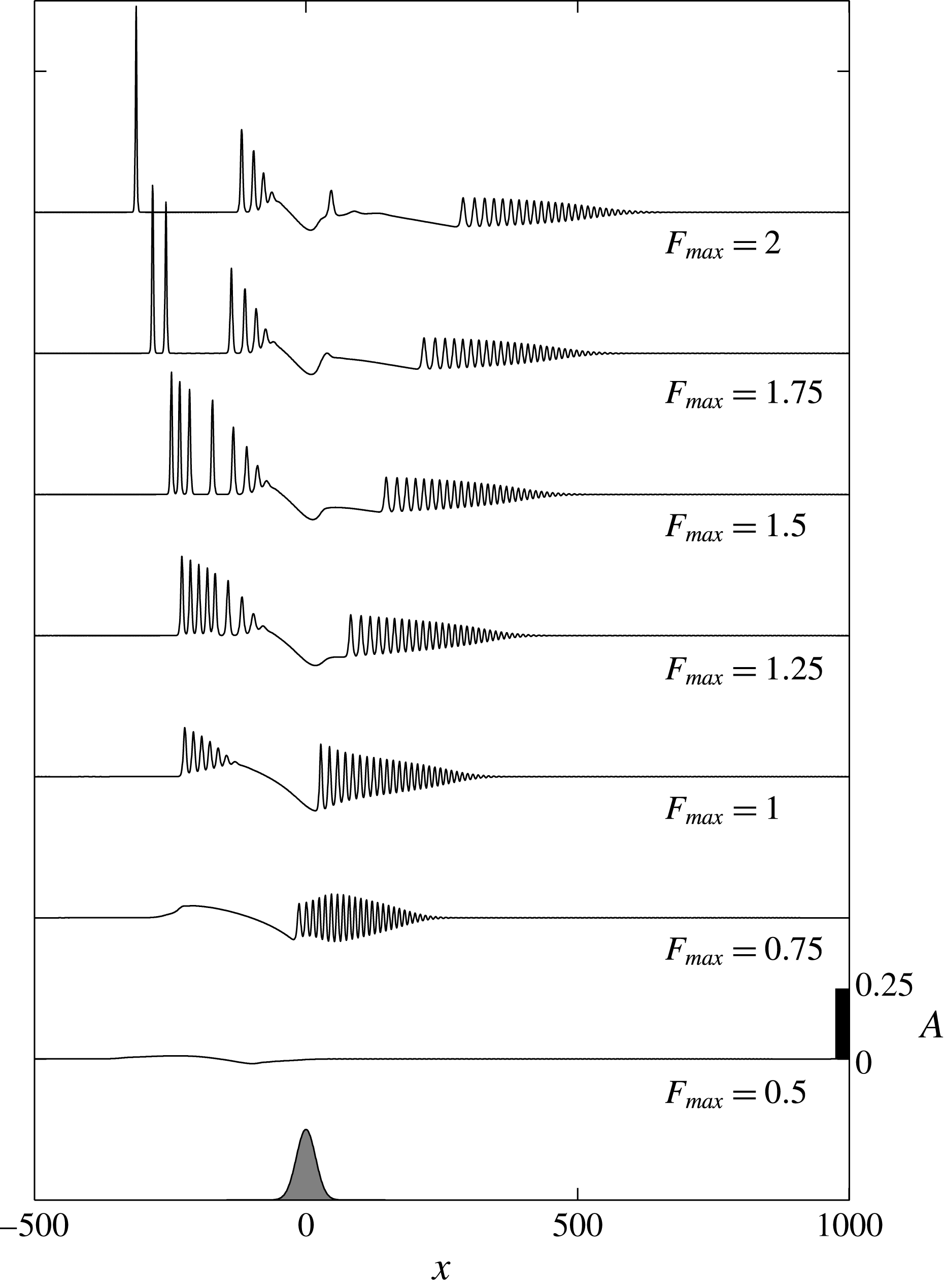
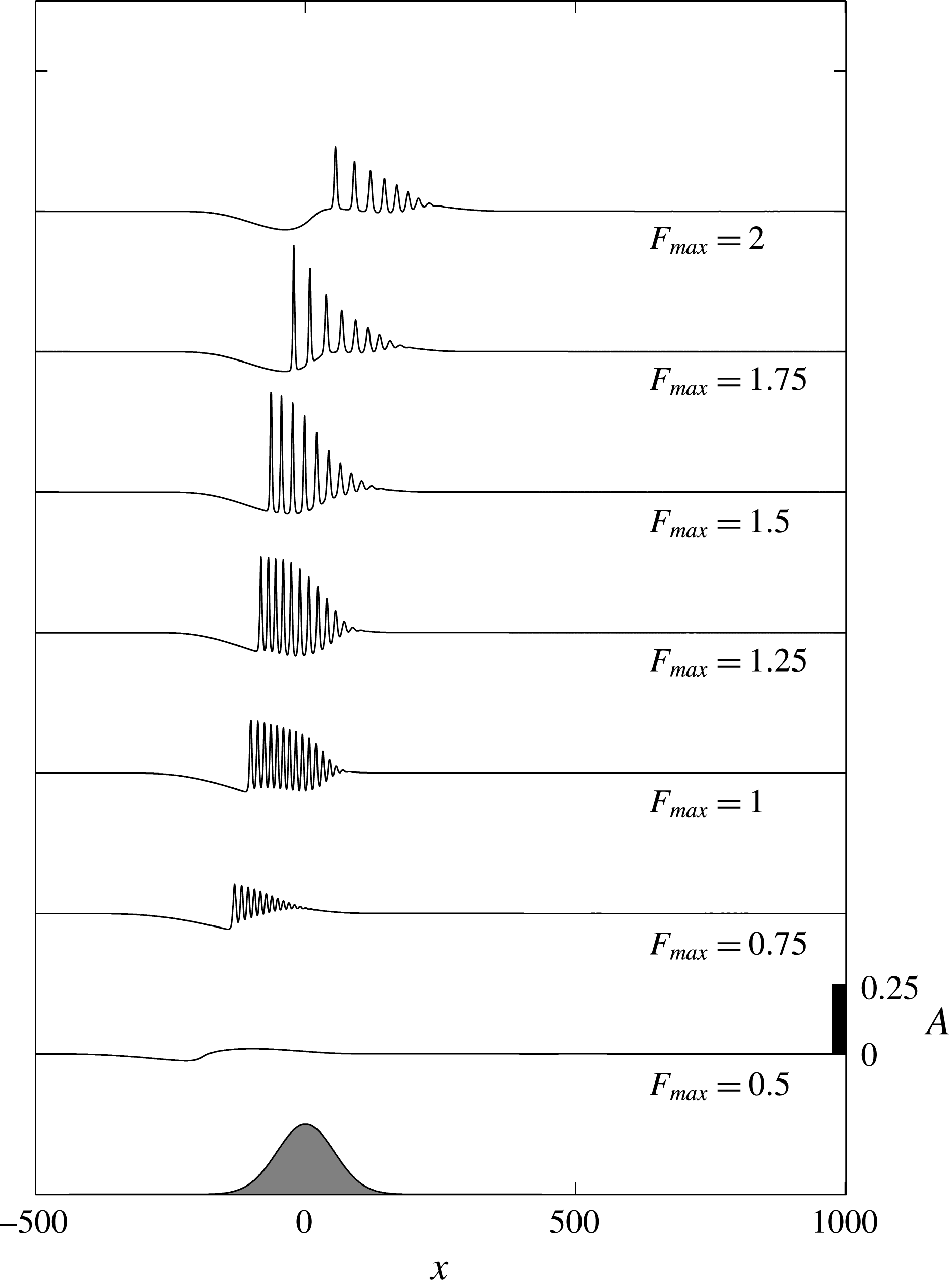
The effect of changing $F_{max}$ is summarised in figure 6 where the solutions at the end of the forcing period, $A(x,t=T/2)$ , are shown for several $0.5\leqslant F_{max}\leqslant 2$ . The other parameters are unchanged. For $F_{max}=0.5$ and $0.75$ , $\unicode[STIX]{x1D6E5}_{max}\lesssim \unicode[STIX]{x1D6E5}_{m}$ and the upstream response is weak since the forcing at most just enters the resonant regime for a very brief period (scenario 1). Runs with $F_{max}=1,1.25$ and $1.5$ ( $\unicode[STIX]{x1D6E5}_{m}<\unicode[STIX]{x1D6E5}_{max}<\unicode[STIX]{x1D6E5}_{M}$ ) all produce upstream and downstream bores (scenario 2). When $F_{max}\geqslant 1.75$ , $\unicode[STIX]{x1D6E5}_{max}\gtrsim \unicode[STIX]{x1D6E5}_{M}$ , the upstream response in particular reflects the two passages through resonance (scenario 3).

Figure 6.

$A(x,T/2)$ for $(b_{M},T,w_{b})=(0.03,1000,25)$ and $F_{max}$ as indicated. The location and shape of the topography (arbitrary amplitude) is shown at the bottom of the plot.

Figure 7.

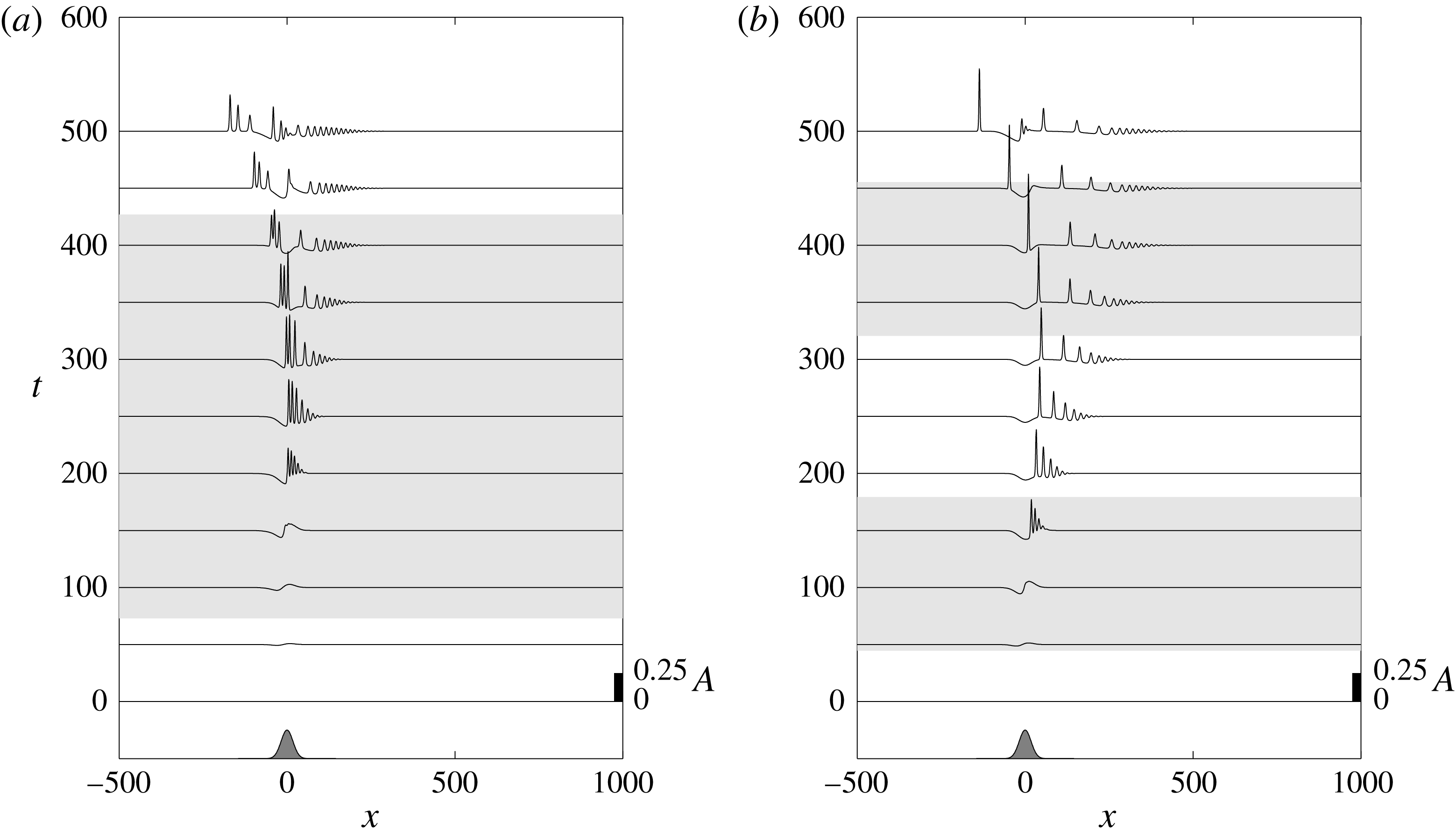
The same as figure 5 but now for $b_{M}=-0.03$ . (a) $F_{max}=1.25$ . (b) $F_{max}=2$ .

Figure 8.

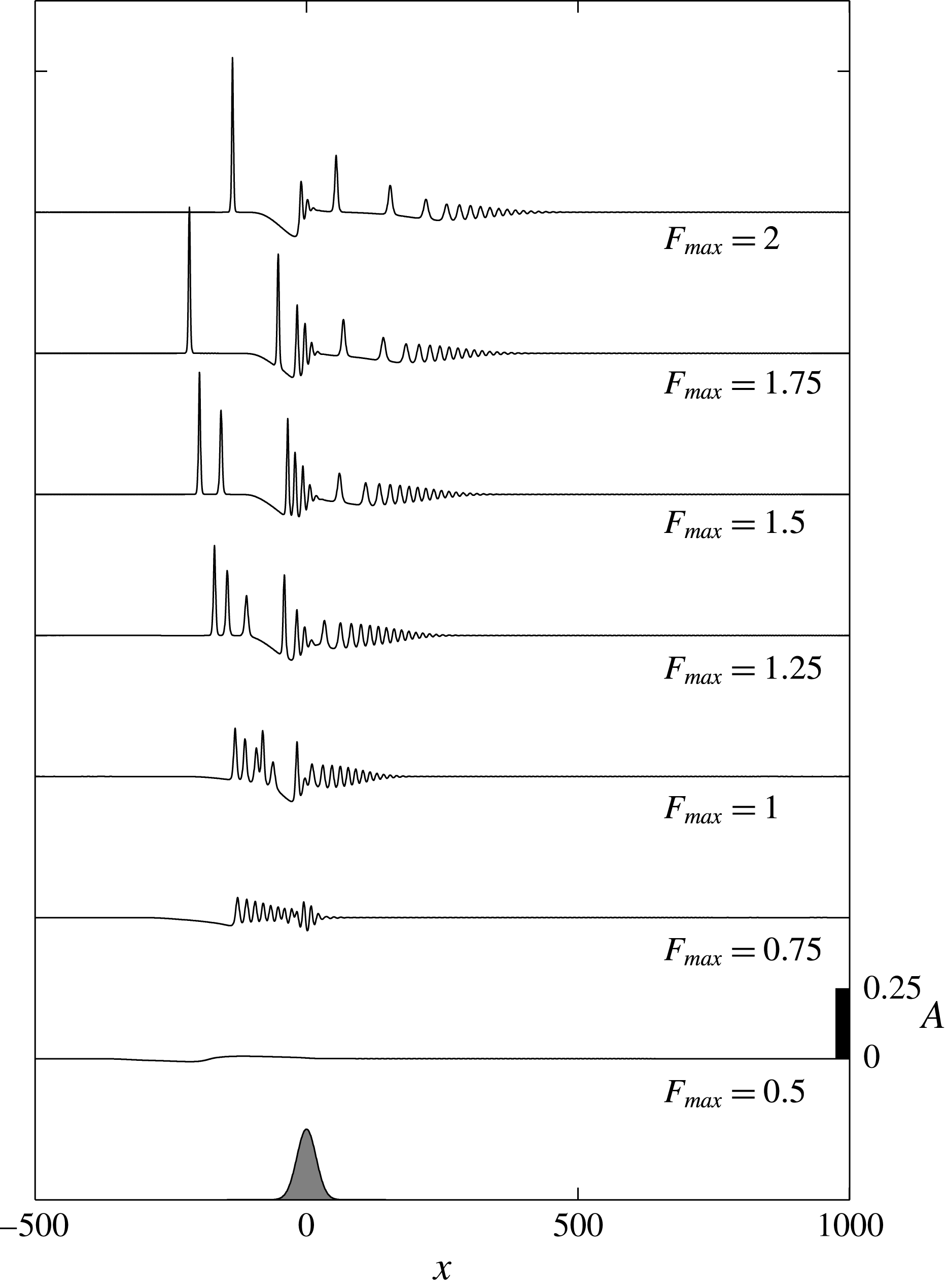
$A(x,T/2)$ for $(b_{M},T,w_{b})=(-0.03,1000,25)$ and $F_{max}$ as indicated.

Solutions for negative forcing $b_{M}=-0.03$ and $F_{max}=1.25$ and $2$ , with $T=1000$ and $w_{b}=25$ unchanged from above, are plotted in figure 7. In both examples the negative forcing results in a downstream undular bore on the increasing phase of the barotropic flow that is released to move upstream as the tidal flow decreases for $t>250$ . Passage of the waves back over the forcing region leads to a more complicated and variable wave field upstream and over the topography than for positive forcing as anticipated from the constant forcing example of figure 2. The effect of further variations in $F_{max}$ , with the other parameters unchanged, on the solutions at $t=T/2$ are shown in figure 8. Again, differences in the response reflect the magnitude of $\unicode[STIX]{x1D6E5}_{max}$ in comparison to $\unicode[STIX]{x1D6E5}_{m}$ and $\unicode[STIX]{x1D6E5}_{M}$ .

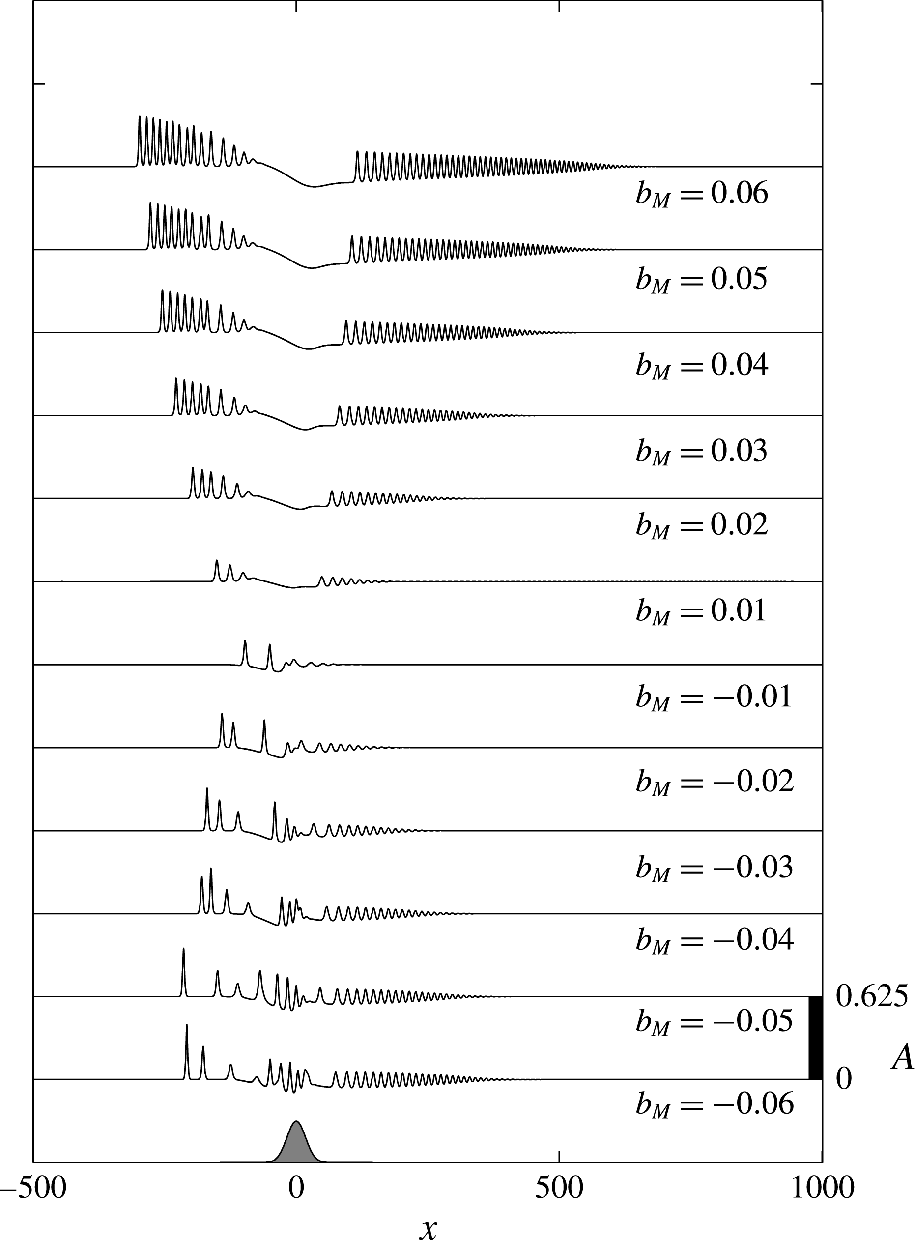
The effect of varying the topographic amplitude, $b_{M}$ , for $F_{max}=1.25$ ( $\unicode[STIX]{x1D6E5}_{m}<\unicode[STIX]{x1D6E5}_{max}<\unicode[STIX]{x1D6E5}_{M}$ ), $T=1000$ and $w_{b}=25$ is shown in figure 9. In addition to the increase of topographic forcing magnitude, increases in $|b_{M}|$ also lead to increased duration of the barotropic forcing residing within the resonant band, hence larger and more numerous waves are generated.

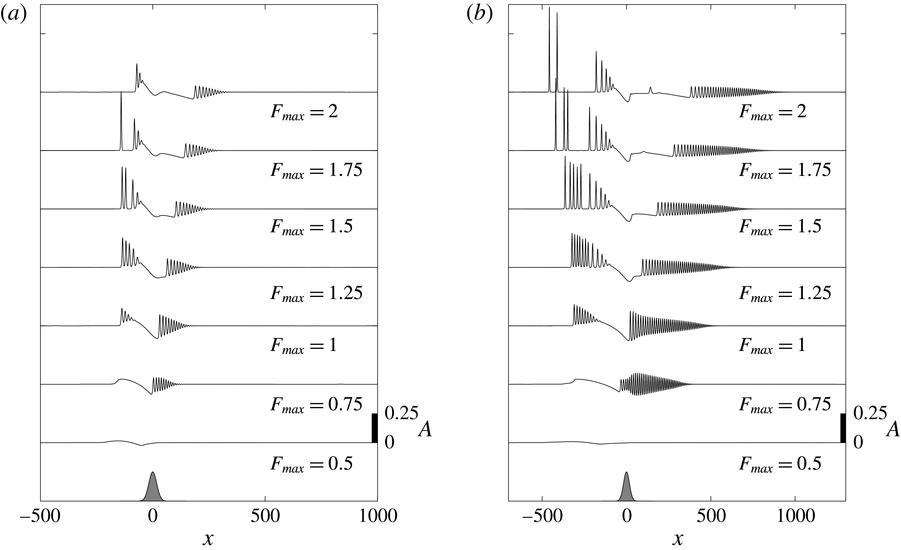
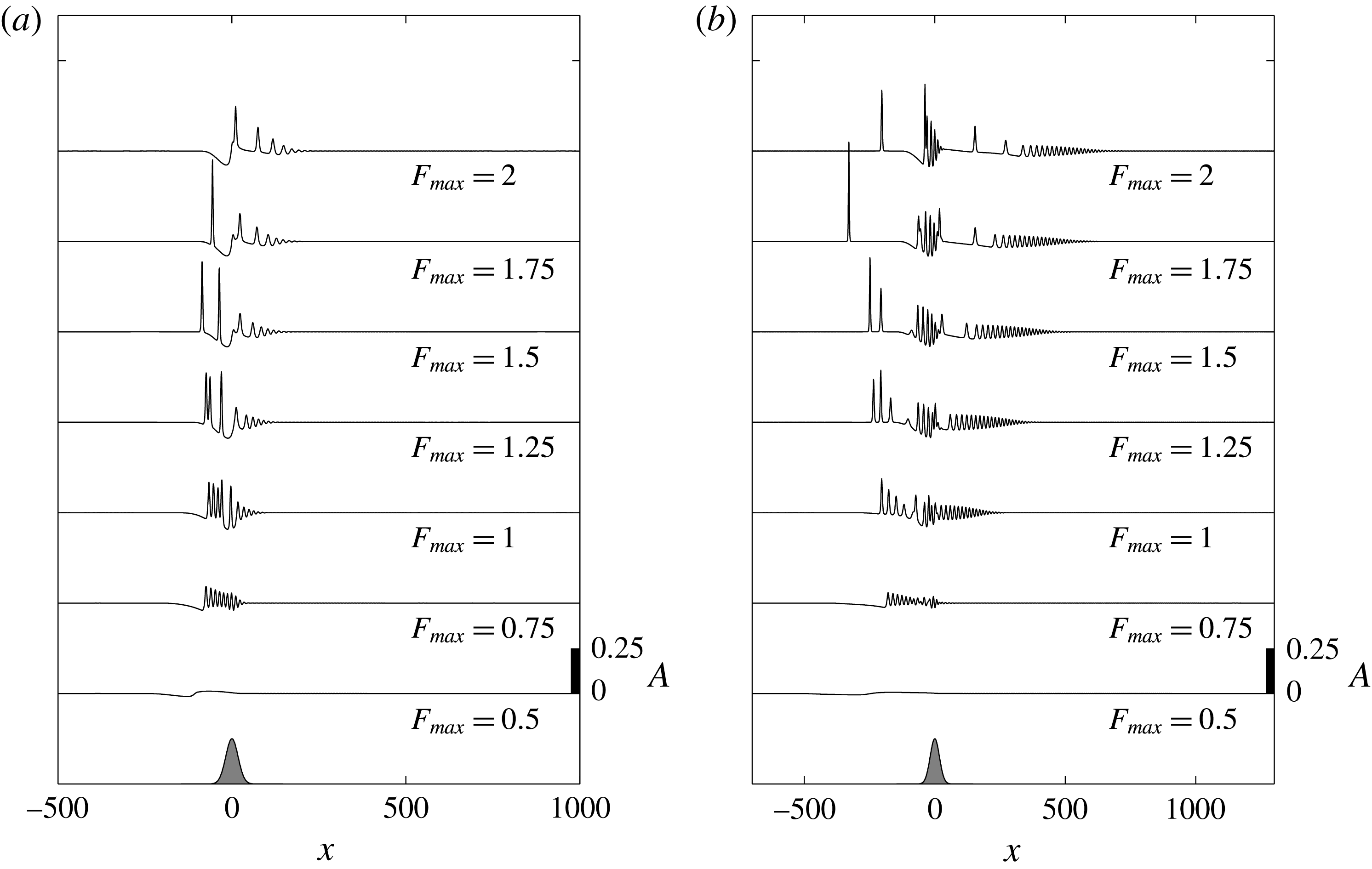
The effect of forcing duration is further illustrated in figures 10(a) and 10(b) which show $A(x,T/2)$ for $T=600$ and $1400$ , respectively. Here $b_{M}=0.03$ , $w_{b}=25$ and $F_{max}=0.5{-}2$ . The same results for $b_{M}=-0.03$ are shown in figure 11.

Figure 9.

$A(x,T/2)$ for $(F_{max},T,w_{b})=(1.25,1000,25)$ and $b_{M}$ as indicated.

Figure 10.

(a) $A(x,T/2)$ for $(b_{M},w_{b})=(0.03,25)$ , $F_{max}$ as indicated, and $T=600$ . (b) The same but now $T=1400$ .

Figure 11.

(a) $A(x,T/2)$ for $(b_{M},w_{b})=(-0.03,25)$ , $F_{max}$ as indicated, and $T=600$ . (b) The same but now $T=1400$ .

Figure 12.

$A(x,T/2)$ for $w_{b}=75$ , $T=1000$ and $b_{M}=0.03$ with $F_{max}$ as indicated.

Figure 13.

$A(x,T/2)$ for $w_{b}=75$ , $T=1000$ and $b_{M}=-0.03$ with $F_{max}$ as indicated.

Figure 14.

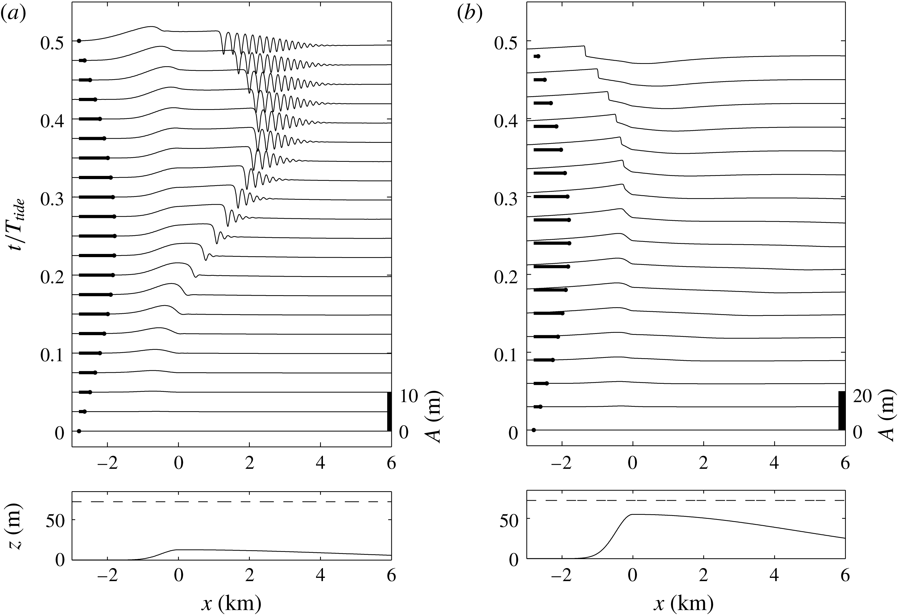
(a) Numerical solution of the fKdV equation (2.13) for a representation of Stellwagen Bank for an ebb tide with $b_{M}/h=0.15$ , $h=85~\text{m}$ and $F_{max}=1.5$ . (b) Numerical solution of the two-layer shallow water equations for a flood tide with the actual topography, $b_{M}/h=0.65$ , and an maximum upstream $F=0.24$ . The lower panels show the topography and the resting interface position. The upper panels show the interface displacement through the tidal forcing. The magnitude and direction of the barotropic flow are indicated by the heavy lines.

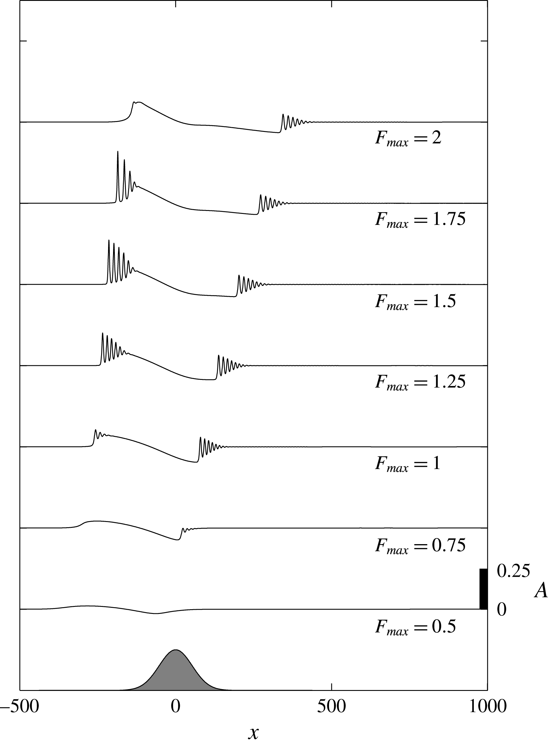
Figure 12 shows the effect of changing the topographic width scale from $w_{b}=25$ to $w_{b}=75$ on $A(x,T/2)$ for $b_{M}=0.03$ . Here $T=1000$ and $F_{max}=0.5{-}2$ . This figure should be compared to figure 6 where $w_{b}=25$ . The broader topography, hence weaker forcing through reduction of $s_{x}$ , results in a weaker upstream and downstream bores for all $F_{max}$ . However, for negative topographic forcing $b_{M}=-0.03$ (figure 13), the upstream propagating bore is eliminated, while the downstream response is increased in comparison to the narrower topography, $w_{b}=25$ , shown in figure 8.

4 Generation of internal undular bores by tidal interaction with asymmetric topography

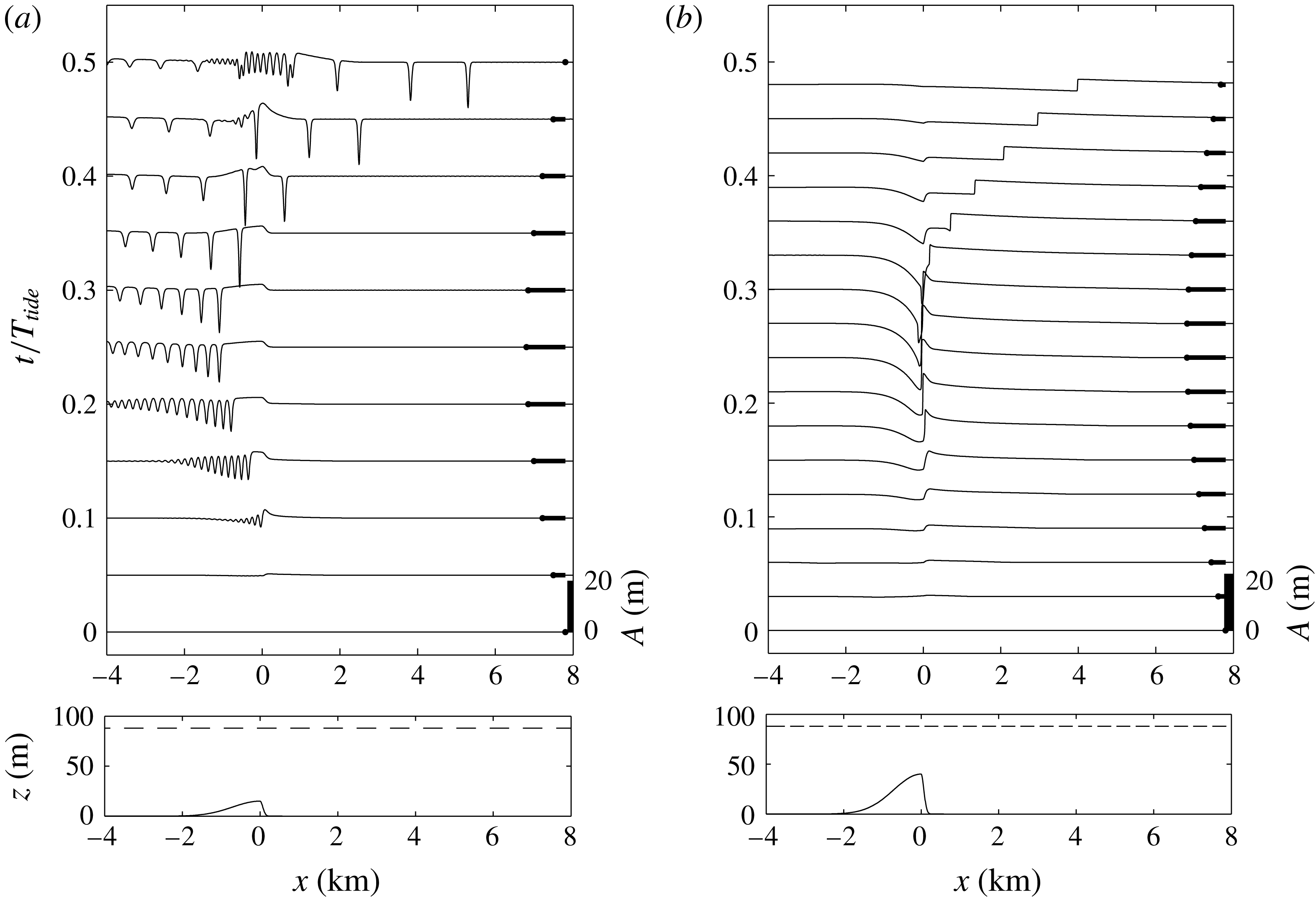
In order to compare this theory in more detail with the generation at actual sites, we note that in practice the forcing topography is often highly asymmetric. This is the case, for instance, with Stellwagen Bank (Scotti et al. Reference Scotti, Beardsley and Butman2007, Reference Scotti, Beardsley, Butman and Pineda2008), where the bank is much steeper on the shoreward side than on the ocean side. In figure 14 we show some simulations representing ebb tide for Stellwagen Bank using a model topography of the same asymmetric shape as the actual topography. The simulations use both the fKdV model (figure 14 a) with a reduced topographic amplitude and a two-layer shallow water model (figure 14 b) with the full topography, both shown in the lower panels. The figure shows the interface evolution over the first half-period of tidal forcing, and for an upper layer depth $h_{1}=12.75~\text{m}=0.15h$ , where the total depth $h=85~\text{m}$ and reduced gravity $g^{\prime }=0.0196~\text{ms}^{-2}$ , giving $c_{0}=0.46~\text{ms}^{-1}$ . The plot is in dimensional units for direct comparison with observations. Because KdV theory is formally limited to small-amplitude topography, the solution in figure 14(a) has the topographic amplitude reduced to $b_{M}=12.75~\text{m}$ ( $15\,\%$ of the total depth) from the actual value of $b_{M}=55~\text{m}$ , and $F_{max}=1.5$ . This topography and tidal amplitude place the forcing in scenario 2 since $\unicode[STIX]{x1D6E5}_{M}=0.54$ . For comparison, figure 14(b) shows the solution of the two-layer shallow water equations (non-dispersive) for the ebb forcing with the actual topography and a maximum upstream $F=0.24$ . This flow produces a maximum $F$ over the sill of approximately $1.5$ . The magnitude and direction of the tidal flow is indicated by the heavy lines in each case. Not surprisingly, the two figures show quantitatively different results and note that the shallow water simulations cannot produce the internal waves, but do show the steepening bores that lead to their formation. However, the qualitative features, especially the general shape and timing of the upstream-moving disturbances, are in good agreement, suggesting that the fKdV model is capturing the essential features of the generation process on this ebb phase of the tide.

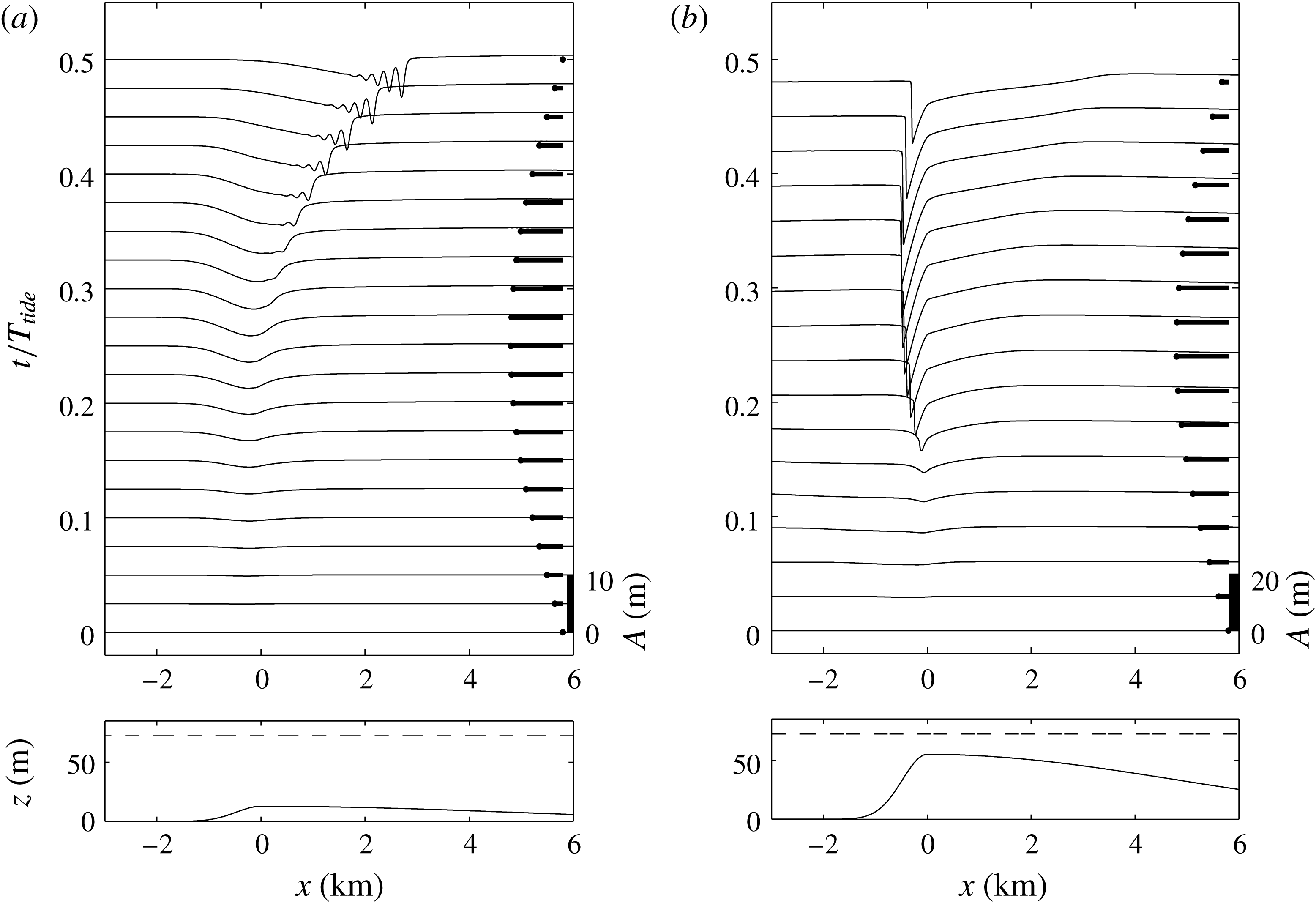
An equivalent pair of simulations for the Stellwagen Bank flood tide are shown in figure 15. Again, there are quantitative differences between the fKdV and shallow water runs (e.g. the strong downstream jump is absent in the KdV simulation while the upstream waves are not present in the shallow water simulation), but the leading upstream disturbance front, at $x\approx 3{-}3.5~\text{km}$ , is captured in both. The effect of the topographic asymmetry leads to substantial changes in the response when compared to the ebb tide examples above.

Figure 15.

The same as figure 14, but now for the flood tide.

Figure 16.

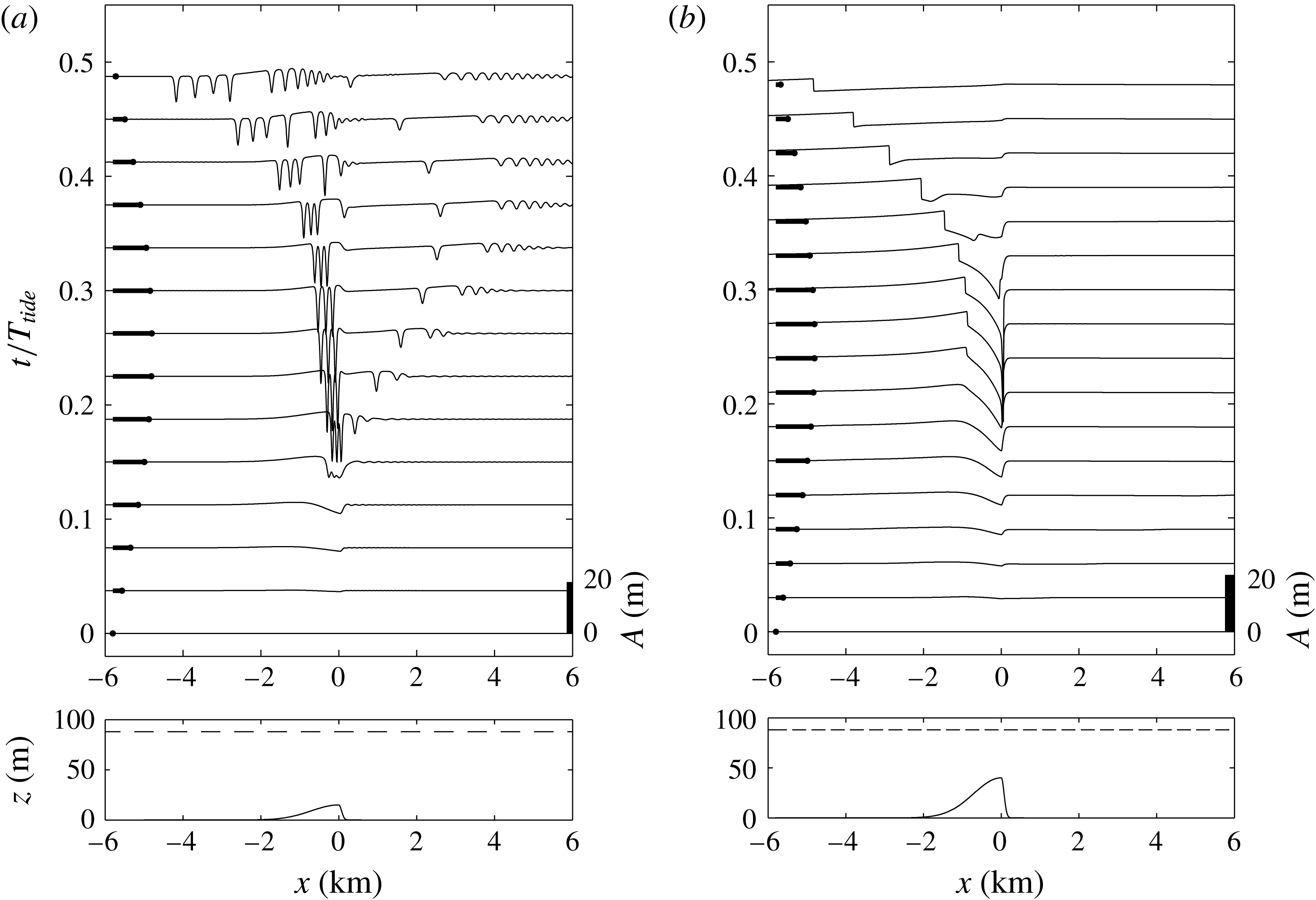
(a) Numerical solution of the fKdV equation (2.13) for a representation of Knight Inlet sill for a flood tide with $b_{M}/h=0.15$ , $h=100~\text{m}$ and $F_{max}=1.5$ . (b) Numerical solution of the two-layer shallow water equations for an ebb tide with the full topography, $b_{M}/h=0.4$ , and an maximum upstream $F=0.66$ . The lower panels show the topography and the resting interface position. The upper panels show the interface displacement through the tidal forcing. The magnitude and direction of the barotropic flow are indicated by the heavy lines.

Figure 17.

The same as figure 16, but now for the ebb tide.

Knight Inlet is another asymmetrical, tidally forced sill (Farmer & Armi Reference Farmer and Armi1999b ; Armi & Farmer Reference Armi and Farmer2002). In figure 16 we show fKdV and shallow water equation simulations for the flood tide. In these calculations the total water depth is taken to be $h=100~\text{m}$ . This is less than the actual depth of approximately $350~\text{m}$ , but is about the depth of the downstream flow separation (Armi & Farmer Reference Armi and Farmer2002; Cummins et al. Reference Cummins, Vagle, Armi and Farmer2003) on flood tide and is thus a reasonable approximation for the active total depth in a two-layered reduction. Again, the topographic shape replicates the steeper landward side of the sill, over which the water is $60~\text{m}$ deep. For these simulations we use an upper layer depth $h_{1}=12~\text{m}$ and reduced gravity $g^{\prime }=0.076~\text{ms}^{-2}$ , giving $c_{0}=0.90~\text{ms}^{-1}$ . Figure 16(a) shows the fKdV simulation for $b_{M}/h=0.15$ and $F_{max}=1.5$ . The strengthening flood tide generates a wave packet that is trapped just upstream of the sill crest until the tide begins to slacken, after which the waves propagate upstream, in qualitative agreement with observations (Farmer & Armi Reference Farmer and Armi1999a ). In the companion two-layer shallow water simulation in figure 16(b) the timing of the upstream disturbance mirrors the waves in the fKdV simulation, although the downstream hydraulic jump is both weaker and shorter lived in the fKdV model. Both simulations highlight the role of a subcritical zone between the upstream jump, or bore, and the hydraulic critical flow at the sill crest, in which the solitary waves develop (Cummins & Armi Reference Cummins and Armi2010). The Knight Inlet ebb tide fKdV and shallow water simulations are shown in figure 17. Again the timing of the upstream propagating disturbances are qualitatively similar in both simulations. We note that in the Knight Inlet observations and numerical simulations, the strong flow deformation over the sill crest with local shear instability, mixing and possible formation of a three-layer flow structure (see Farmer & Armi (Reference Farmer and Armi1999a ), Cummins et al. (Reference Cummins, Vagle, Armi and Farmer2003), Cummins et al. (Reference Cummins, Armi and Vagle2006) and Cummins & Armi (Reference Cummins and Armi2010) for instance) is not captured of course, in either the fKdV model or in the two-layer simulations. Nevertheless, the formation of the upstream wave field is at least qualitatively captured, suggesting that this is essentially determined by the passage of the Froude number through criticality as we have described in § 3 and as has been previously suggested by Farmer & Armi (Reference Farmer and Armi1999a ) and Stastna & Peltier (Reference Stastna and Peltier2004).