Not Guilty? Agriculture in the 1920s and the Great Depression

GIOVANNI FEDERICO

doi:10.1017/S0022050705000367

Not Guilty? Agriculture in the 1920s and the Great Depression

Published online by Cambridge University Press: 22 November 2005

GIOVANNI FEDERICO

Show author details

GIOVANNI FEDERICO: Affiliation:
Professor, Department of History and Civilization, European University Institute, Via Boccaccio 121, 50133 Firenze, Italy. E-mail Giovanni.Federico@iue.it.

Article contents

Abstract
AGRICULTURAL “OVERPRODUCTION” AND THE DEPRESSION: THE “REAL” STORY
AGRICULTURE AND THE DEPRESSION: THE “MONETARY” STORY
CONCLUSION: WHY DID AGRICULTURAL PRICES FALL DURING THE DEPRESSION?
References

Rights & Permissions

Abstract

Agricultural distress in the 1920s is routinely quoted among the causes of the Great Depression. This article challenges the conventional wisdom. World agriculture was not plagued by overproduction and falling terms of trade. The indebtedness of American farmers, a legacy of the boom years 1918–1921, did jeopardize the rural banks, but the relation between their crises, the banking panic of 1930, and the Great Depression is tenuous at best.

Information

Type: ARTICLES
Information: The Journal of Economic History , Volume 65 , Issue 4 , December 2005, pp. 949 - 976
DOI: https://doi.org/10.1017/S0022050705000367 [Opens in a new window]
Copyright: © 2005 The Economic History Association

The Great Depression has arguably been the major peacetime macroeconomic shock in world economy since the start of modern economic growth. From 1929 to 1933 the GDP per capita fell by a third in the United States and by about 9 percent in the Atlantic economy.¹

Data are from Maddison, World Economy. The Atlantic economy includes Western Europe and its off-shoots (see the list of countries in Table 3).

In spite of decades of research, its causes remain still controversial: Ben Bernanke has felicitously called the issue, the “Holy Grail” of macroeconomics.²

Bernanke, Essays, p. vii

Why did a recession start in 1929 and, above all, what transformed a mild downturn into the worst economic crisis since the Industrial Revolution, with far-reaching political and social consequences?

Most of the answers to these questions can be framed in two different interpretative traditions, the “real” and the “monetary” (or “financial”) story.³

For some additional references, see Balderston, “Introduction,” pp. 1–6, for the “real” story; and Calomiris, “Financial Factors”; and Randall “Overview,” pp. 9–14, for the monetary one.

Although disagreeing on most issues, they share a negative view of the conditions of agriculture during the “Roaring Twenties.” For instance, Peter Temin states that, after the war, “agriculture had gone from prosperity to poverty.”⁴

Temin, Lessons, pp. 11 and 55. See also Temin, Did Monetary Forces, pp. 2 and 146–48.

However, the two traditions single out different sources of weakness: the “real” story focuses on the structural disequilibrium between supply and demand in the world market for agricultural products, and the “monetary” one on the high level of debt of American farmers. In both stories, agriculture was highly vulnerable to any cyclical downturn, and its crisis was a major component of the depression. This stylized fact is routinely repeated in general books about the economy of the interwar years: for instance, according to Patricia Clavin, “the troubled health of agriculture, especially in eastern and southern Europe, was the most serious drag on European economic growth.”⁵

Clavin, Great Depression, p. 78. See. also Kindleberger, World, pp. 70–74 and 90–92; Romer, “World War One,” p. 110; Pollard, Peaceful Conquest, pp. 500–01; Eichengreen, Golden Fetters, p. 227; Bairoch, Victoires, vol. 3, pp. 36–38; Koning, Failure, pp. 163–84; Foreman-Peck, History, pp. 187–88; Feinstein, Temin, and Toniolo, European Economy, pp. 71–76; James, End, pp. 63 and 105; Sheingate, Rise, pp. 76–77; and Findlay and O'Rourke, “Commodity Market,” pp. 44–45.

This article challenges this view. The conditions in agriculture on the eve of the depression, although far from ideal, were not as bad as suggested by the received wisdom. Therefore, the collapse of agricultural prices in 1930–1933 and the ensuing devastating crisis were not a necessary consequence of the farmers' behavior in the previous decade. Given the clear distinction between the two stories, they will be dealt with separately.

AGRICULTURAL “OVERPRODUCTION” AND THE DEPRESSION: THE “REAL” STORY

The Causes of the Depression

According to the “real” story, agriculture contributed both to the outbreak of the depression in 1929 and to its catastrophic worsening in the second half of 1930. In the short run, the downturn was accelerated by the poor conditions of the balance of payments of agricultural exporters such as Australia or Argentina. Vladimir Timoshenko primarily blames the poor 1929 crop, which reduced their exports, whereas William Lewis and Barry Eichengreen stress the effect of the 1928 American monetary squeeze on these heavily indebted countries.⁶

Timoshenko, World Agriculture, pp. 66–76; Lewis, Economic Survey, p. 58; and Eichengreen, Golden Fetters, pp. 227–28.

The drying-up of capital imports forced these countries first to liquidate their stocks of primary products, starting a downward spiral in agricultural prices, and ultimately to abandon the gold standard. On a different tack, James Hamilton shows that futures markets—usually quite efficient in predicting agricultural prices—erred spectacularly throughout the Great Depression, and Pierre Siklos speculates that the (unanticipated) price fall in 1929 might have triggered the depression.⁷

Hamilton, “Was the Deflation,” pp. 158–62; and Siklos, “Understanding the Great Depression,” pp. 35–36. Hamilton shows how the (poor) predictions of future markets for agricultural commodities also shaped expectation about the aggregate price level.

The alleged disequilibrium was, however, a long-run problem, dating back to World War One.⁸

The gist of this interpretation was put forward in two major works by the League of Nations, Agricultural Crisis (which voiced the opinions by agricultural experts from some 30 countries) and Course (a report written by Bertil Ohlin, with the advice of other eminent economists such as Hayek or von Morgestern) and in the highly influential book by Timoshenko, World Agriculture, pp. 8–32. See also Genung, Agricultural Depression, p. 21; Arndt, Economic Lessons, pp. 10–12; and Lewis, Economic Survey, pp. 151–52. See also the more skeptical views by Aldcroft, From Versailles, pp. 223–28; and Bernstein, Great Depression, pp. 9–12 and 103.

In W. A. Lewis's words, “both domestic [i.e., American] and international agricultural prices had been falling since the mid-1920s, capacity having grown faster than demand.”⁹

Lewis, “W. Arthur Lewis,” p. 9.

During the war farmers—especially those from Western Settlement countries—had substantially increased their productive capacity, augmenting inputs and adopting several innovations, most notably mechanical ones.¹⁰

“Western Settlement” countries include the United States, Canada, Australia, and New Zealand.

Demand had been growing slowly, as the consumption of agricultural products was price- and income-inelastic, and the European population was increasing much more slowly than before the war. The excess production either ended up in stocks, financed with short-term loans, or, given the low elasticity of demand for food, caused prices of agricultural products to decline well before the outbreak of the depression. Farmers were thus highly vulnerable to any additional decrease in prices, even a relatively mild one. In a recent paper, Jakob Madsen sums up nicely this conventional wisdom: “the overproduction of agricultural products and the mounting stocks made agricultural prices vulnerable to shocks in demand, international lending and the international financial system.”¹¹

Madsen, Agricultural Crises, p. 356.

This disequilibrium allegedly accounted for the precipitous fall in agricultural prices during the depression.

How did the fall in agricultural prices affect the rest of the economy? Agrarian economists in the early 1930s used a proto-Keynesian argument: the fall in farmers' income reduced economy-wide demand. Lewis points out that the fall in prices benefited consumers—so that the net effect on domestic demand was likely to be small.¹²

Lewis, Economic Survey, pp. 46 and 56–57, and “W. Arthur Lewis,” p. 10. See in the same vein Fleising, “United States”; Aldcroft, From Versailles, p. 236; Kindleberger, World p. 91; and Atack and Passel, New Economic View, pp. 594–96. Temin (Lessons, p. 56) suggests that the net domestic effect might have even been positive.

In contrast, he stresses that the decrease in prices created expectations of further decline, depressing investments, and that it reduced the purchasing power of exporters of primary products, forcing them to abandon the gold standard. As Eichengreen puts it, the ensuing contraction in exports was “another nail in the coffin of American prosperity.”¹³

Eichengreen, Golden Fetters, p. 246.

Madsen has recently estimated the macroeconomic effects of the price decline from 1929 to 1933 and has found them to have been really substantial. The fall in absolute agricultural prices accounted for almost all the deflation, and the fall in relative agricultural prices accounted directly for a sizeable share of the decrease in aggregate demand (about a half for consumption and between one-fourth and one-third for investment).¹⁴

Madsen, Agricultural Crises. The figures are obtained from the coefficients of a set of dynamic equations for 15 countries in 1929–1936. They refer to the direct effect only, omitting the additional effects via the depression of land prices and the reduction in farmer's wealth.

This article will not try to replicate Madsen's work, nor will it try to assess the relative importance of overproduction versus slow growth in demand as cause of the (alleged) disequilibrium. The article will instead focus on the existence of a disequilibrium, a necessary, though not sufficient, condition for the whole “real” story. To this end, it will look at the evidence on prices, production, and stock in the 1920s. Before discussing the available data, it is necessary to stress how narrowly focused the traditional narrative is. First, it deals almost exclusively with the countries of the Atlantic economy. African and Asian countries appear only as suppliers of selected tropical imports, such as coffee and rubber. Second, even the coverage of temperate agriculture is decidedly selective, in all likelihood according to the available data. Cereals and industrial crops have a paramount role whereas livestock products are given very little attention. Last but not least, the existence of the disequilibrium is mainly inferred from the decline in nominal prices and the increase in stocks for specific commodities. Production data are seldom quoted, and sometimes dismissed, as they do not show any spectacular increase in the 1920s, with the exception of rubber and perhaps silk.

The Evidence: Prices

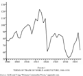
The data on relative prices do not confirm the conventional wisdom. Figure 1 reports the index of world agricultural terms of trade (ratio of prices of agricultural products to the unit values of manufactures) by Enzo Grilli and Maw Cheng Yang.¹⁵

The agricultural prices index is a weighted average of indices for food (0.85) and nonfood agricultural raw materials (0.15). Unfortunately, their series do not extend before 1900. From 1910 to 1929, prices declined at the yearly rate of –1.54 percent (significant at 15 percent).

It shows a rise in the first years of the century, with a wartime peak in 1917, followed by a sudden collapse. The terms of trade recovered only partially from the 1920–1921 crisis: on the eve of the Great Depression, the average was some 15 percent lower than in 1910–1913. This comparison is, however, somewhat unfair, as the prewar prices were historically very high. Indeed, the 1910–1914 price level (“parity”) was to assume a mythical status in the following years: achieving it was the goal of the Agricultural Adjustment Act, the cornerstone of the New Deal agricultural policy. In fact, the “terms of trade” in the late 1920s were still 10 percent higher than in the early 1900s.

FIGURE 1 TERMS OF TRADE OF WORLD AGRICULTURE, 1900–1938

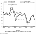
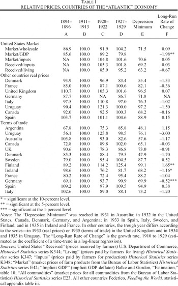
Grilli and Yang provide very few details about the computation of their indices. However, methods of computation can matter, as Figure 2 shows. It reports five series of agricultural prices for the United States, which are computed as ratios of four different basic series (farm-gate prices, wholesale price indices, implicit GDP deflator). Prices fluctuated a lot during the war and the 1920s: the wartime rise and subsequent fall was as great as the fall and subsequent recovery during the depression. Yet, in the long term, agricultural prices have remained constant. On the eve of the depression, they were back to their prewar level and, with one exception, the rates of change from 1910 to 1929 are not significantly different from zero (Table 1). These data cast serious doubts about the conventional wisdom, at least for the United States.

FIGURE 2 REAL AGRICULTURAL PRICES, UNITED STATES 1910–1938

What about other countries? Table 1 reports data on the agricultural terms of trade (ratio of prices of agricultural products/manufactures) and real agricultural prices (prices of agricultural products/overall price indexes) for as many countries of the Atlantic economy as possible at some relevant benchmark years. As expected, the terms of trade move more than real prices, which include the agricultural products in the denominator. The trends differ substantially among countries, possibly reflecting differences in coverage and methods of estimation of the series. The prices in 1927–1929 were lower than in 1910–1913 in six out of 13 countries and than in 1894–1896 in two only (Ireland and Denmark). As shown in column E of Table 1, in only three countries (all in Europe) was there a statistically significant downward trend in terms of trade from 1910 to 1929. In all other cases, short-term fluctuations swamped long-term trends. Price trends were even more favorable in the rest of the world.¹⁶

From 1911–1913 to 1927–1929, terms of trade improved in Punjab (+19 percent), Thailand (+11 percent), India (+4.5 percent), Korea (+4 percent), and Japan, while they decrease in Egypt (–1 percent), China (–1.2 percent), and above all Taiwan (–45 percent). Federico, Feeding the World, statistical appendix table iii.

In short, there was no large-scale “structural deflation,” to use Kindleberger's words, in the 1920s.¹⁷

Kindleberger, World, p. 93.

Nor was there a widespread worsening in 1929, which could account for the outbreak of the depression à la Timoshenko and Eichengreen. From 1928 to 1929 the terms of trade fell in Argentina (by 6 percent) and Uruguay (by 2 percent) and in the majority of European countries, but they improved in Canada and Australia as well as in the United States. These modest changes in prices contrast with the veritable collapse after the outbreak of the Great Depression (Figure 2 and column F of Table 1): this fall is likely to have influenced the perception of precrisis experience.

The Evidence: Production and Stocks

At first glance, the change in stocks seems to be strong evidence for the conventional wisdom. Both the series by Timoshenko (from 1923 onwards) and that by the League of Nations (from 1925 onwards) show a rapid increase in the late 1920s, at yearly growth rate of 7.5 percent and 11.3 percent respectively.¹⁸

Timoshenko, World Agriculture, table 10; and League of Nations, Memorandum, 1938–1939. Both sources reports estimate for different dates of the year. The growth rates in the text are computed with 1 June indexes for the period 1925–1929.

However, these indices are seriously flawed. First, they cover a small set of products—cereals, textile fibers, and tropical products, which happened to be the most subject to the (alleged) overproduction.¹⁹

At least in the case of Timoshenko's index, this effect is worsened by a bizarre weighting, which bears no relationship at all with the composition of agricultural production. Textile material (cotton and raw silk) account for 40.4 percent of the total; tea, coffee, and sugar for 36.8 percent; and wheat for the remaining 22.2 percent. The League of Nations does not provide information on the weighting of its series.

Second, the basic series may be not representative. Most of them refer to so called “visible supply,” the stocks in ports and public warehouses (sometimes only in some countries or markets). They omit stock held by farmers, by traders in their own warehouses, and by processing industries. According to the League of Nations, the ratio of visible stocks to “world total stocks” increased for wheat and sugar, although not for cotton.²⁰

From 1925 to 1929, the ratio for cotton remained stable, whereas those for wheat and sugar grew from 43 to 51 percent and from 34 to 48 percent, respectively (League of Nations, Memorandum, 1938–1939).

Therefore, the series counting the “visible supply” overvalue the growth in total stocks. Last but surely not least, the level of inventories in the late 1920s was not exceptional if compared with production or consumption. Wheat stocks accounted on average for 14.7 percent of world output from 1922 to 1928, whereas from 1890 to 1913 they had amounted to 17.6 percent of production.²¹

Output is from Bennet, “World Wheat Crops”; Davies “World Wheat Situation,” table 1; and Farnsworth, “Wheat,” table 2 (the series exclude Russia). The stock of wheat at 1 August is from Farnsworth, “World Wheat Stocks,” table 1. The author points out (pp. 57–58) that the increase of the share of output from the southern hemisphere increased the equilibrium stock/output ratio. The stocks were not unusually large in proportion to output for coffee as well. The ratio was 50.5 percent in 1883–1913 (Ukers, All About Coffee, p. 274) and 37.6 percent on average in 1923–1929 (League of Nations, Agricultural Crisis, table 9). It rose to 84.6 percent in 1928/29, which anyway was not the highest on record.

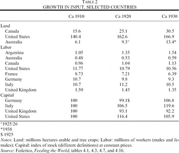
Inventories rose to 24.5 percent in 1929, after the 1928 bumper crop and remained around a quarter of output throughout the 1930s.

The available data on the use of inputs, although incomplete (Table 2), rule out a reckless expansion of productive capacity in the 1910s and 1920s. The number of workers remained stable or even declined in most countries, capital increased by 5–10 percent and the stock of land in only a few overseas countries was clearly on the rise. To be sure, productive capacity might have increased thanks to technical progress, and indeed the sources of the 1930s often quote mechanization as a major breakthrough brought about by the war. But the number of tractors remained very low as late as 1930, and the growth in Total Factor Productivity, although somewhat faster than before the war, was still modest. In the United States, the rate from 1919 to 1929 was 1.2 percent per year, corresponding to a cumulative increase by 13 percent.²²

Kendrick, Productivity Trends, table 34. See Federico, Feeding the World, chapter 5 and statistical appendix table 4 for the productivity growth and table 4.11 for the number of tractors.

From this standpoint, the real watershed was to be World War Two. Last but not least, the increase in the productive capacity in the Atlantic countries was at least partially offset by the disappearance of Russian supply from the world market after the Revolution.²³

Russia accounted for 28 percent of world exports of cereals in 1909–1913 (Stern, “Century”) and for 12 percent of “world” gross output in 1913 (Federico “Growth,” table 5).

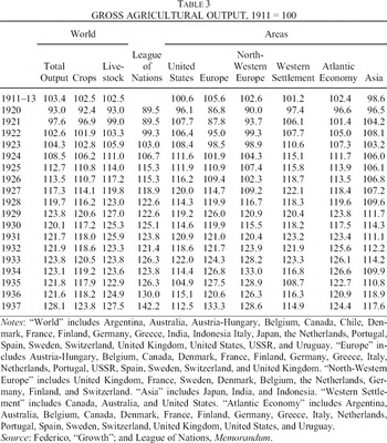
The evidence of a slow increase in productive capacity is consistent with the data on production (Table 3). In the 1920s and 1930s the League of Nations published a first index of world gross agricultural output, which, however, omits dairy and meat.²⁴

League of Nations, Memorandum. The gross output is the total production available for human consumption or industrial processing after the deductions for seeds, cattle feeding, and other farm uses.

A more recent estimate covers all products, for 25 countries at their 1913 borders.²⁵

Federico “Growth.” The article covers the whole Atlantic economy, plus Eastern Europe (Russia and Austria-Hungary) and several South American and Asian countries.

It shows some substantial differences in performance among areas, but clearly production did not increase fast. On the eve of the depression, the gross output was about 15–20 percent higher than before the war. This increase is far from impressive. In the 20 years from the early 1890s to 1911–1913, a period that is widely regarded as a golden era for farmers, production grew by a third and doubled in the countries of Western Settlement. If the 1870–1913 growth rate had been sustained in the 1910s and 1920s, then by 1929 the output would have been about 10 percent higher than its actual level.²⁶

See Federico, “Growth,” table 4.

The Disequilibrium Between Supply and Demand: An Estimate

The potential disequilibrium in the year t can be estimated as

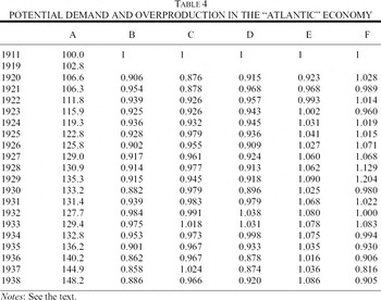
where S is an index of productive capacity and D is an index of potential demand—all expressed as a ratio to an equilibrium year. The data on productive capacity are too scarce to estimate S, which thus will be proxied with actual production. This is tantamount to assuming that productive capacity was fully utilized and short-term fluctuations of output reflected only the vagaries of the weather. The potential demand is computed as

where P is population and Cp is per capita consumption of agricultural products,

where A is a survival bundle of consumption (constant over time), Y is GDP per capita, [prod ] is an index of “world” real prices of agricultural products, and α and β are the relevant elasticities.

The equilibrium year is assumed to be 1911. The baseline estimate of R (Table 4, column B) is the ratio of aggregate production of the Atlantic economy (Table 3) to the baseline estimate of demand (Table 4, column A). This latter is computed by assuming a moderately inelastic demand, with α 0.6 and β –0.3.²⁷

The index of real prices is computed as a weighted average of country series of Table 1, plus the ratio of food/consumer prices in the United States (U.S. Department of Commerce, Historical Statistics, series E 137/E135). These countries are fairly representative, as they accounted for about 85 percent of the population of the “Atlantic” economy. The national indices are weighted by population: using the country shares of gross output in 1913 (Federico “Growth,” table 6) instead does not affect the results. These series are wholesale prices, and thus they might not be representative of retail ones, which consumers faced. It is, for instance, possible that falls in prices of raw products such as wheat did not pass through to consumers because of the rise in processing costs (wages, etc.) or because of the market power of food companies. In the United States, the price of bread fluctuated much less than that of wheat (U.S. Department of Commerce, Historical Statistics, series E 188 and K 508). The divergence between wholesale and retail prices was a major concern for agricultural experts (League of Nations, Agricultural Crisis). The GDP and population are from Maddison, World Economy

The results show no disequilibrium: if any, production was inferior to potential demand, but differences are within the plausible margin of error. The other columns of Table 4 show that this result is quite robust to changes in assumptions. Column C uses the index of production by the League of Nations, column D assumes zero price elasticity, and column E assumes both income and price elasticity to have been zero—i.e., that aggregate demand changed only as much as population. Only in this last case, an extreme version of Lewis's scenario, did actual production exceed potential demand all over the 1920s, with a widening gap. However, the assumption of zero income and price elasticities does not seem really plausible for the whole agricultural demand, which included “luxuries” such as sugar, coffee, and livestock products.²⁸

As an alternative, one could hypothesize that elasticity was positive, but consumers adjusted spending to their expected permanent income. Clearly, no one could have predicted the Great Depression—so permanent income in the 1920s could be computed as the average of the years 1921–1929 or as an interpolation of income growth in the same years. In both cases, the production/demand ratio is lower than in the baseline case.

Finally, column F refers to wheat only—the product most affected by overproduction according to the conventional wisdom.²⁹

Wheat production is computed by summing up gross output in Argentine, Australia, Canada, the United States, Belgium, Denmark, Finland, France, Germany, Ireland, Italy, the Netherlands, Norway, Portugal, Spain, Sweden, Switzerland, and the United Kingdom, plus imports from Russia (Stern, “Century”). All the data are from Mitchell, International Historical Statistics, table D2—except for those for Belgium (Blomme, Economic Development), Italy (ISTAT, Sommario), and Portugal (Lains, personal communication). Prices are proxied by the ratio of price of wheat in the United States (U.S. Department of Commerce, Historical Statistics, series K 508) to wholesale price index (series E 53). The elasticities are assumed to be 0.2 for income and –0.1 for prices. The “overproduction” disappears totally if Atlantic demand is compared with total world production, from Bennett “World Wheat Crops.”

Total production in the Atlantic economy did exceed demand only after 1926. On top of this, the estimate is biased upwards by the omission of imports from Russia: adding them to the equilibrium (1911) production level would reduce the productive capacity S. Consequently, the index R would exceed one only in 1927–1928.

The “Real” Story: An Assessment

The statistical evidence discussed so far refers to agriculture as a whole, and thus it does not rule out differences by crop. According to Grilli and Yang, in the late 1920s the “terms of trade” for agricultural raw materials were 30 percent lower than before the war.³⁰

Grilli and Yang, “Primary Commodity Prices.”

In the United States the real prices of cereals and meat never regained the pre-war level, whereas those of dairy products, fruits, and even cotton exceeded it by the late 1920s.³¹

Prices of corn, wheat, and cotton are from U.S. Department of Commerce, Historical Statistics, series K504, K508, and K 555. Other products are from Strauss and Bean “Gross Farm Income,” series 85, 86, and 90. All prices are deflated using the index of the cost of living for farmers, U.S. Department of Commerce, Historical Statistics, K347.

In most countries livestock products fared better than crops.³²

See Federico, Feeding the World, table 3.7.

The effect on farmers' incomes depended on the scope for substitution among products. This substitution was limited in some cases by environmental constraints (climate, lack of irrigation water) or, for tree-crops such as rubber, by the lag between planting and the start of commercial production.³³

The production of the trees planted in the boom years of the early 1920s glutted the market in the late 1920s (Aldcroft, From Versailles, pp. 228–29). Even if the initial investment in a plantation was totally amortized, plantations should not have continued to produce if prices did not cover variable costs.

However, many other farmers succeeded in adjusting their crop mix to changes in relative prices. In fact, the share of livestock products out of total gross output was rising in most countries and in the “world” total.³⁴

The share of livestock products of total “world” output increased from 43.6 percent in 1911–1913 to 45.8 percent in 1928–1930. The sum of fruit and livestock products (meat, dairy products, and eggs) increased from 62.2 percent of U.S. gross output in 1919–1921 to 70.1 percent in 1928–1930 (these data come from Strauss and Bean, “Gross Farm Output,” tables 10 and 27).

The same reasoning holds true for exporting countries: only a few of them were inescapably trapped in the wrong specialization. Moreover, exporting countries were not yet seriously damaged by European protectionism, as tariffs were still relatively low. According to Heinrich Liepmann, the average duty on cereals was lower in 1913 than in 1927 in nine countries out of 15, including France and Italy.³⁵

Liepmann, Tariff Levels, table AI (potential tariff levels). The duty was also lower in 1927 than in 1913 in the majority of countries for fruit and vegetables, whereas it was higher for the other categories such as livestock, animal foodstuffs, and other foodstuffs. The differences were anyway quite small. Furthermore, barriers to trade were even lower in the early 1920s (League of Nations, Agricultural Crisis, pp. 17–21; Clavin, Great Depression, pp. 81–86; and Federico, Feeding the World).

On the other hand, disadvantaged farmers (and countries) complained loudly, and their plight looms large in the traditional account of the crisis.

Summing up, the evidence rules out a major disequilibrium. This result should not be really surprising, if one considers how farmers in Western settlement countries behaved according the traditional story. They allegedly increased their productive capacity under the twin assumption that demand was to increase as fast as before the war and, crucially, that European agriculture would be unable to satisfy it. One can admit a collective error in prediction under the exceptional wartime circumstances, but the conventional wisdom implies that they went on erring throughout the 1920s, even after the great shock of 1920–1921 and the return to normalcy in international economic relations. In other words, they were betting on a price rebound, which did not materialize. Such a collective misjudgement is hardly credible, especially as farmers had the option to migrate to cities, where the economic growth offered plenty of job opportunities.³⁶

In the United States, the market for labor was well integrated in the 1920s (Alston and Hatton “Earnings Gap”), and 0.63 millions farmers migrated to cities each year from 1921 to April 1930 (U.S. Department of Commerce, Historical Statistics, series C 78).

In contrast, the behavior of farmers would be perfectly rational if prices had remained stable in the long run. This seems to have been the case: all the evidence suggests a slow but steady growth in production matching the slow but steady growth in demand.

AGRICULTURE AND THE DEPRESSION: THE “MONETARY” STORY

The “Monetary” Story

Agricultural distress would play an important role in the “monetary” story of the Great Depression if it caused or contributed to cause the banking panics. As is well known, Milton Friedman and Anna Schwartz, in their classic book A Monetary History of the United States, argue that the banking panic of October 1930, poorly managed by the Federal Reserve, turned the initial downturn into the Great Depression.³⁷

Bank failures caused a substantial and unexpected reduction in the money stock, which the Federal Reserve was unable or unwilling to contain (Friedman and Schwartz, Monetary History pp. 299–311 and 338–341). See the reappraisal by Hamilton, “Causes”; or by Cole and Ohanian “Great Depression,” pp. 16–19. Other scholars, such as Bernanke (“Non Monetary Effects”), stress a different channel of transmission. The fall in supply of banking services and the more cautious lending policy of surviving institutions forced households to save more.

Farmers' indebtedness could cause a nationwide banking panic if: first, it caused a substantial number of farmers to fail; second, these failures caused banks that had financed farmers to fail; and, third, the failure of rural banks either triggered the panic (a case of strong exogeneity) or helped to propagate it (weak exogeneity). This section will discuss these three conditions, after having briefly outlined the origins of the indebtedness of American farmers in the 1920s. Consistent with the overall “monetary” story, the section will focus uniquely on the United States, although the connection between indebtedness and banking panics elsewhere in the world is worthy of research. In fact, farmers were also quite heavily indebted in other countries, such as Germany, and the occurrence of a banking panic in a country worsened its performance during the depression.³⁸

See Bernanke, “Macroeconomics”; and, on the causes of banking crises in other countries, Grossman, “Shoe.” On the indebtedness of German farmers, see League of Nations, Agricultural Crisis, pp. 171–72.

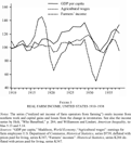
The Gathering of the Storm: Farmers' Income and Indebtedness in the 1920s

On the eve of the depression, the condition of American farmers was not terrible, although surely not very good. The 1920s had been quite an eventful decade (to say the least) for them (Figure 3). Farmers had profited handsomely from the war-time boom and were hard hit by the fall in prices. From 1917 to 1921, their real income fell by 55 percent—i.e., as much as from 1929 to 1932.³⁹

See for an account of the crisis Shideler, Farm Crisis, pp. 36–52; and Johnson, “Postwar Optimism.”

In the 1920s it crawled back, and at the end of the decade it was back to its prewar level. However, farmers had lost ground relative the rest of the economy and also relative to their own employees. GDP per capita was 30 percent higher than before the war and agricultural wages were some 10 percent higher. This difference with their own employees may have affected the farmers' status and self-perception more than the comparison with far-away city dwellers. These gaps were to widen during the depression—only to bounce back with the New Deal and the Agricultural Adjustment Act.

FIGURE 3 REAL FARM INCOME, UNITED STATES 1910–1938

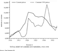
However, the real problem for American farmers was indebtedness. The real stock of debt had been growing steadily since the late 1890s but it really soared from 1918 to 1921 (Figure 4).⁴⁰

Data are from U.S. Department of Commerce, Historical Statistics: on debt after 1910 (as of 1 January) series K361 and K376–K380; on net personal savings, series F 547; both deflated with prices received by farmers (series K 344). From 1897 to 1909, the real stock increased by 10 percent (nominal stock is from Goldsmith, Study, series M27 and A 23, deflated by wholesale prices of agricultural products from U.S. Department of Commerce, Historical Statistics, series E 42).

Farmers borrowed for a variety of purposes (including the speculation on purebred animals) but mainly for purchasing land. In those three years, the nominal price of land increased by a third and real prices by 61.5 percent.⁴¹

The nominal value of land is from Lindert, “Long-Run Trends,” table 1, deflated with prices received by farmers (U.S. Department of Commerce, Historical Statistics, series K 344). These yearly figures are unadjusted for the quality change related to the westward expansion. Lindert's adjusted figures are at ten-year intervals, and therefore unsuitable for a short-term analysis. The bias from the use of yearly data is, anyway, very small: from 1915 to 1930 unadjusted real prices fell by 39.2 percent and adjusted ones by 36.9 percent.

Farmers' net financial wealth decreased by more than 9.4 billion (1911) dollars—i.e., by roughly 1.3 times the value of the 1919 gross output.⁴²

For the estimate of the gross output see Federico, “Growth.”

Net savings fell by some 2.5 billion and debt increased by almost 7 billion—i.e., by 156 percent in real terms (and by 45 percent in nominal terms). These figures undervalue the actual increase in debt, as they refer to all loans from institutions and to mortgage-backed loans from individuals. They thus omit the unsecured loans from individuals (“junior” mortgages), which might have accounted for about a quarter of the total.⁴³

The main, official, mortgage usually amounted to about half the value of the farm, whereas these “junior” mortgages, backed with personal promissory short-term notes, could supply up to a further 40 percent in some cases (Johnson “Post-War Optimism,” pp. 184–85). These loans accounted for 15 percent of total farm debt in the 1970s (U.S. Department of Commerce, Historical Statistics, p. 478). It is conservatively assumed that they amounted to about a quarter of the known total in the 1920s.

FIGURE 4 TOTAL DEBT OF AMERICAN FARMERS, 1910–1938

The fall in prices, from June 1920, dramatically worsened the financial conditions of farmers. Real interest rates jumped to almost 50 percent and interest payments on mortgage-backed loans rose to 16.6 percent of farmers' income.⁴⁴

Interest on mortgages is from U.S Department of Commerce, Historical Statistics, series K 372, income series K 284, plus interest payments. On the credit crunch, see Shideler, Farm Crisis, pp. 52–58; and for the policy of the Federal Reserve, see Metzler, History, pp. 114–15.

Adding payments on other mortgages, the total burden might have exceeded a quarter of total income.⁴⁵

This figure is estimated assuming that unsecured loans paid the same interest rate as mortgage-backed ones. This is a conservative estimate (Clarke, Regulation, table 3.1).

Last but not least, farmers incurred huge capital losses: the nominal price of land fell by almost 30 percent from 1921 to 1922.

Throughout the rest of the 1920s, the stock of nominal debt and the interest/income ratio decreased slowly but steadily. By 1929 the debt was 13 percent lower in nominal and 25 percent lower in real terms than it had been eight years before. However, this reduction was brought about almost exclusively by foreclosures, which increased from 3.2 percent of farms in 1913–1920 to 10.7 percent in 1921–1925 and to 17.7 percent in 1926–1929.⁴⁶

Alston, “Farm Foreclosures,” table1; and Goldsmith, Study, table M 27. The data also include distress sale without formal procedure.

In fact, the outstanding debt had fallen by a total of 2.4 billion current dollars while, according to Raymond Goldsmith, foreclosures had wiped out 2.8 billion of debt.⁴⁷

From 1922 to 1929, total financial assets remained constant (only increasing by 9 million), tax arrears increased by 110 million, mortgage-backed debts fell by 1.1 billion, and other debts fell by 1.3 billion (Goldsmith, Study, tables M 28, A-53, A-54, and A.65). The source reports figures at 1930 prices, which are converted in current prices with the index of prices received by farmers (U.S. Department of Commerce, Historical Statistics, series K 344). The author estimates the total value of debt on foreclosed farm assuming that each mortgage amounted to three-quarters of the average one.

Thus farmers who had managed to stay in business were heavily indebted. On the eve of the Great Depression the debt/output ratio, inclusive of the unsecured loans from individuals, might have been around 125 percent and the interest/income ratio around a sixth. These are nationwide averages, but the level of indebtedness varied a lot across the country—roughly increasing from East to West.⁴⁸

Alston “Farm Foreclosures,” table 2; and Hamilton, “Causes.”

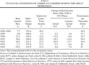
In other words, many American farmers were still haunted by the overhang of the 1921 boom and bust and this may have been an important source of weakness once the storm broke.

Farmers' Indebtedness and the Great Depression

There is little doubt that indebtedness worsened the conditions of farmers during the Great Depression (Table 5). The nominal stock of debt fell somewhat from the precrisis level, but much less than gross output—so that the debt/output ratio doubled. Real interest rates soared, interests payments gobbled a growing share of income, and foreclosures (with some lag) increased to unprecedented heights.⁴⁹

These figures are subject to a contrasting bias. They understate the burden of interests as they omit non-mortgage-backed loans and they overstate the burden, as they neglect interest rate delinquency, which was, on the contrary, quite diffused.

As column D.2 shows, farmers' real income would have fallen by “only” 18 percent instead of by almost 30 percent if they had not had to pay interest (column D.1). Lee Alston shows that the percentage of foreclosures from 1926 to 1940 by state was positively related to the percentage of mortgaged farms: a 10 percent increase in this latter increased the average rate of foreclosure rate by 1.4 percent, i.e., by 7.5 percent at the average.⁵⁰

Alston, “Farm Foreclosures.” The rate of foreclosures was also positively related to the fall in income and to the extent of the previous land boom (measured with the increase in improved acreage from 1910 to 1925 and the increase in land prices from 1900 to 1912).

Thus the first of the three conditions is hardly controversial

The effect of the farmers' financial plight on the banking system depended, ceteris paribus, on the share of credit to agriculture in the banks' total assets. From this point of view, the situation of the banking system as a whole was not so troublesome. In fact, most mortgages had been subscribed by individuals, insurance companies, and other non-banking institutions.⁵¹

By 1929, “individual and others” accounted for 47 percent of secured loans; insurance companies for 22 percent; Federal land banks, state credit agencies, and joint-stock land banks (monitored and guaranteed by the state) for 20 percent; and “commercial” banks for only 10 percent (including a tiny 1 percent for mutual saving banks) Goldsmith, Study, tables A-61 and A-62.

By 1929 assets of “commercial” banks included 1 billion dollars for secured loans and 2.6 billion for unsecured loans to farmers—small sums compared with the total assets of the banking system (62 billion dollars) and also with those of “state [chartered] commercial banks” (some 34 billion), which included rural banks.⁵²

U.S. Department of Commerce, Historical Statistics, series X 684, less assets of private banks (series X 686). The total assets of “non-national banks,” which also included mutual savings, totalled 45 billion—10.4 of which was (urban and rural) real estate (U.S. Department of Commerce, Historical Statistics, series X 657 and 658).

However, it is highly likely that credit to farmers was mainly held by rural banks and that it accounted for a sizable share of their assets. Rural banks were very vulnerable to agricultural crises. Most states did not allow them to open branches, and thus to diversify their assets, and on top of this they had no right of support from the Federal Reserve.⁵³

See Alston, “Why do Banks”; and White, Regulation, pp. 14–17 and 127–32.

In case of foreclosure, most losses were borne by holders of “junior mortgages,” but banks did not escape unscathed. For instance, a bank that had lent a farmer half the sum to purchase land in 1920–1921 was bound to lose, on average, about 14 percent of the value of this asset if the farm was subject to foreclosure in 1933, when nominal land prices were about a third of their purchase level. But these losses from foreclosures were only a part, possibly a small one, of total ones. It is likely that banks postponed or forfeited altogether the payment of mortgage instalments before starting the procedure of foreclosure, which they considered only as a last resort.⁵⁴

Alston, “Farm Foreclosure Moratorium.”

Last but not least, banks (surely mostly rural ones) bore the burden of the decline in the total deposits of farmers from 2.9 billion dollars in 1929 to 1.6 in 1933.⁵⁵

Goldsmith, Study, table A 53. These figures include deposits to other institutions. Rural banks were hit more than others, as depositors tended to shift funds to city banks—the so called seepage (Wicker, Banking Panics, pp. 101–02).

All these blows can account for the high mortality among “state [chartered] banks.” Between 1930 and 1933 some 6,865 of them, two out of five state banks operating in 1929, failed. The rate of failure for the other categories of banks was “only” about 25 percent.⁵⁶

U.S. Department of Commerce, Historical Statistics, series X 580, X 683, and X 685 for the number of banks in 1929, and X 741 and X 743 for the number of failed banks. See Hamilton, From New Day, pp. 148–65, for the hesitant and ultimately failed attempts to help the distressed banks.

Thus, the two first conditions are established well enough: the crisis did jeopardize the financial situation of farmers and, as a consequence, of rural banks. The third condition, the relationship between the conditions of rural banks and the overall banking crisis (most notably the 1930 panic), is much more difficult to prove. Friedman and Schwartz, consistent with their overall interpretation, opt for a strong exogeneity. The 1930 panic was “neither foreseeable nor inevitable,” and it was not a consequence of a previous worsening in the “quality of loans.” They state that “a contagion of fear spread among depositors, starting from the agricultural areas, which had experienced the heaviest impact of bank failures in the 1920s.”⁵⁷

Friedman and Schwartz, Monetary History, p. 308.

They do not pursue this hint, focusing instead on the case of the Bank of the United States, a New York bank with large loans in real estate. However, it is not difficult to hypothesize that an unanticipated fall in prices or perhaps a poor crop convinced depositors in some agricultural areas that the local bank could not sustain the farmers' losses, starting a wave of panic. How plausible is this scenario? Elmus Wicker, in his book on The Banking Panics of the Great Depression downplays the relevance of the 1930 panic for the Depression and the role of agriculture in it. He blames the failure of Caldwell and Co., a Tennessee bank, which had overextended itself in a purchasing spree, whereas the subsequent waves of panic in 1931 and 1933 originated in big cities (Chicago and Detroit).⁵⁸

Wicker, “Reconsideration” and Banking Panics, pp. 32–36 and 152–54. See also Metzler, History, pp. 325–26.

Wicker's account would thus relieve agriculture of any responsibility for starting the banking panics. David Hamilton disagrees, arguing that the failure of Caldwell and Co. accounted for only a small share of total bankruptcies. The majority of failures were caused by the fall in cotton and tobacco prices and by the drought, which hit many Southern states in 1930.⁵⁹

Hamilton, “Causes.” His view is indirectly supported by Hamilton's results about price expectations (Hamilton “Was the Deflation”). The less anticipated price falls were, the more likely that they triggered a panic.

These conflicting assessments are not surprising: by definition, the hypothesis of strong exogeneity is difficult to prove, or disprove, conclusively.

On the other hand, some econometric works suggest that agricultural distress and indebtedness can explain, at least partially, the rate of bank failures. In the 1920s agricultural distress, measured by the rate of foreclosures, had been the main determinant of differences among states in the rate of bank failures.⁶⁰

Alston et al., “Why do Banks,” p. 421. See also Wheelock, “Regulation,” on Kansas; and Fischer, American Banking Structure, pp. 199–210.

Temin finds that the share of income from cotton and wheat of state GDP was positively related to the banking crisis in 1930 and 1931—but not in 1929.⁶¹

Temin, Did Monetary Forces, pp. 83–90. He uses several measures of crisis—number of failures, proportion of failed banks, and so on. The concentration of failures in the South explains the strong effect of the variable share of cotton. The relationship is somewhat weaker for wheat, although wheat states had been the most hit by the wave of foreclosures of the 1920s. This shift in the trouble spots may have been a coincidence (or the consequence of the drought), but it might also reflect the effect of foreclosures, which had weeded out the weakest farmers in the wheat-growing states.

In a short paper, Clifford Thies and Daniel Gerlowski show that the share of failed banks was positively related to the proportion of real estate loans on their assets in 1927–1929 and 1930–1932, but not in earlier periods.⁶²

Thies and Gerlowski, “Bank Capital.” The rate of failure is negatively related to the size of the banks. The regression omits all real variables—including state income.

The effect is reinforced if the variable is interacted with indexes of the borrowers' distress such as the share of foreclosed farms or the change in land prices. Kris Mitchener finds a negative relation between the fall in farm values from 1920 to 1930 and the rate of bank failures by county.⁶³

Mitchener, “Bank Supervision.”

These results might support the hypothesis of weak exogeneity, but, unfortunately, none of them is really conclusive. A strong causal relationship in the 1920s might not have held true in the 1930s. Temin uses an indirect measure of distress, whereas Thies and Gerlowski and Mitchener do not discriminate between panic and nonpanic years.⁶⁴

Thies and Gerlowski (“Bank Capital”) consider all real estate loans, not just agricultural ones, in the denominator of their key explicative variable (on the role of loans to real estate in the Depression also see Eichengreen and Mitchener “Great Depression”).

A paper by Charles Calomiris and Joseph Mason, by far the most detailed one in this literature, tackles brilliantly all these methodological issues.⁶⁵

Calomiris and Mason, “Fundamentals.” On the causes of failure among national banks also see White, “Reinterpretation.”

They find very little if any evidence of a negative effect of agricultural specialization on the survival of banks (and of a major role of panic as a cause of bank failure). Unfortunately, it refers to banks subject to the Federal Reserve supervision—i.e., the national ones and a minority of state-chartered banks. Therefore, it cannot be conclusive either.

Summing up, the evidence for the “monetary” story seems insufficient. The war and postwar boom of the 1920s had saddled farmers with a huge amount of debt, which greatly reduced their ability to weather the fall in nominal prices ten years later. The agricultural crisis jeopardized the financial situation of the rural banks, and many of them failed. But it is quite difficult to prove the third condition—the existence of a causal link between the crisis of rural banks and the overall banking panic. The best guess rules out a strong relation between the crisis in the countryside and the outbreak of the 1930 panic. The poor conditions of rural banks are likely to have contributed to the overall financial crisis during the depression, but their specific contribution is difficult to disentangle from the more general boom and bust in real estate.

CONCLUSION: WHY DID AGRICULTURAL PRICES FALL DURING THE DEPRESSION?

Relative agricultural prices did fall dramatically in almost all countries during the Great Depression (Table 1), while world agricultural production remained roughly constant (Table 3). In the conventional wisdom, these trends would be quite easy to explain as a dramatic consequence of the long-term disequilibrium, but as Table 4 shows, there is even less evidence of overproduction after the outbreak of the crisis than before. How, then, can the price fall be squared with the no-disequilibrium scenario? There are three possible answers to this question.

First, the Total Factor Productivity may have grown faster in agriculture than in the rest of the economy. This hypothesis seems highly unlikely. The gap in TFP growth rates between sectors would have to be implausibly large. Moreover, the available data suggest that from 1929 to 1937 TFP grew more slowly in agriculture than in the rest of the economy.⁶⁶

The TFP growth of farming from 1929 to 1937 (0.8 percent) was the lowest among the main sectors of the American economy according to Kendrick (Productivity Trends, table 34). Field (“Most Technologically Progressive”) argues that Kendrick's figures underestimate nonfarm productivity growth.

Thus, if anything, productivity trends would cause the relative prices of agricultural products to rise.

Second, agriculture might have been hit more than other sectors by the fall in the supply of banking services.⁶⁷

Bernanke, “Non Monetary Effects.” He remarks that big corporations could finance their investments with their funds, but this argument, however, does not apply to cash-strapped farmers. For a more critical view, see Bernstein, Great Depression.

When the local bank failed, farmers had to resort to city banks, which, given informational asymmetries and the poor reputation of agriculture, rationed credit or charged high real interest rates.⁶⁸

The supply of credit to farmers was rationed by legislation for foreclosure moratoria, enacted by several states in 1932–1934 (Alston “Farm Foreclosure Moratorium”). For some additional evidence of the insufficient supply of credit to agriculture and for the measures to increase it, see Hamilton, From New Day, pp. 153–62.

This would augment the transaction costs for farmers, and the increase would show up in a widening gap between prices received by farmers and (urban) wholesale prices of agricultural products. Indeed in the United States, the former did decline a little more than the latter, but the difference is too small to account for more than a small fraction of the fall in agricultural prices.⁶⁹

From 1929 to 1932, prices received by farmers fell by 41.5 percent, while wholesale prices of farm products by 38.2 percent (U.S. Department of Commerce, Historical Statistics, series K 344 and E42). The fall might reflect productivity improvements in transportation and marketing.

It is a fortiori even less plausible that this effect extended to other countries, where agriculture was less dependent on credit.

The third, and most plausible, hypothesis focuses on the asymmetry between agriculture and the rest of the economy. Agriculture was a competitive sector and, in the peculiar conditions of the depression, its elasticity of supply was bound to be low. In fact the opportunity cost of farmers' labor was extremely low as it depended on the expected wages in other sectors. Real wages were rising, but the high rate of unemployment made the prospect of emigration to cities hardly attractive.⁷⁰

The yearly net migration from the countryside (U.S. Department of Commerce, Historical Statistics, series C 78) to cities totaled 0.63 million from 1921 to April 1930 and 0.64 million from 1934 to 1939, but only 61,000 in 1931. From April 1931 to April 1933, 3.0 million people left farms and 3.74 returned, with a net immigration of 763,000 persons.

Thus farmers were likely to go on producing as long as revenues covered their variable costs plus a minimum income for the purchase of indispensable consumer goods. In this situation, demand shocks caused prices to fall. In contrast, in the rest of the economy demand shocks caused a fall in output because prices were sticky. A long interpretative tradition, dating back to Keynes, attributes this feature to wage stickiness, determined by the power of trade unions, by the existence of welfare benefits or by the existence of long-term labor contracts.⁷¹

See, for example, among the many works, Bernanke and Carey, “Nominal Wage Stickiness”; Bordo, Erceg, and Evans, “Money”; the discussion by Cole and Ohanian, “Great Depression,” pp. 19–21; Kehoe and Prescott, “Introduction,” pp. 12–13; and Madsen, “Length,” pp.239–41.

Another interpretation, first suggested by Steindl and recently revived by Madsen, blames limited competition in manufacturing.⁷²

Madsen, “Prices” and “Length.”

To sum up, this article largely exonerates agriculture from its alleged responsibility for the depression. The acquittal is complete for the charge of “overproduction” in the “real” story, and likely for the “monetary” story. In spite of their reckless borrowing spree, especially during the postwar boom, farmers were more a victim of the depression than a cause of it.

This article has been discussed in seminars at the Humboldt University (Berlin), Pompeu Fabra (Barcelona), Copenhagen and Carlos III (Madrid). The author thanks all participants, the editor, and two referees for their comments. They are not responsible for the remaining errors. He also thanks Jeff Williamson for having shared his database on terms of trade.

References

Aldcroft Derek. 1987. From Versailles to Wall Street. 2nd edition. Hardmonsworth: Penguin,

Alston Lee. (1983): “Farm Foreclosures in the United States During the Interwar Period.” This JOURNAL 43, no. 4 885– 903.Google Scholar

Alston Lee. (1984): “Farm Foreclosure Moratorium Legislation: A Lesson from the Past.” American Economic Review 74, no. 3 445– 57.Google Scholar

Alston Lee, Wayne A. Grove, and David C. Wheelock. (1994): “Why do Banks Fail? Evidence from the 1920s.” Explorations in Economic History 31, no. 4 409– 31.Google Scholar

Alston, Lee, and Timothy J. Hatton. (1991): “The Earnings Gap Between Agricultural and Manufacturing Laborers, 1925–1941.” This JOURNAL 51, no. 1 83– 99Google Scholar

Arndt H. W. 1963. The Economic Lessons of the Nineteen-Thirties. 2nd edition. London: Frank Cass,

Atack Jeremy, and Paul Passel. 1994. A New Economic View of American History. 2nd edition. New York and London: W.W. Norton,

Bairoch Paul. 1997. Victoires and deboires. Paris: Gallimard,

Balderston Theo. 2003. “Introduction: the ‘Deflationary Bias’ of the Interwar Gold Standard.” In The World Economy and National Economies in the Interwar Slump, edited by Theo Balderston, 1– 26. Basingstoke: Palgrave,

Balke N. S., and R. J. Gordon. 1989: “The Estimation of Pre-War GNP: Methodology and New Evidence.” Journal of Political Economy 97, no. 1 38– 92.Google Scholar

Benedict Murray. 1953. Farm Policies of the United States, 1790–1950. New York: The Twentieth Century Fund,

Bennett M. K. 1933: “World Wheat Crops 1885–1932” Wheat Studies 9, no. 2 239– 74.Google Scholar

Bernanke Ben. 2000. Essays on the Great Depression. Princeton, NJ: Princeton University Press,

Bernanke Ben. 1995: “The Macroeconomics of the Great Depression: A Comparative Approach.” Journal of Money, Credit and Banking 26, no. 1 1– 28.Google Scholar

Bernanke Ben. 1983: “Non Monetary Effects of the Financial Crisis on the Propagation of the Great Depression.” American Economic Review 73, no. 3 257– 76.Google Scholar

Bernanke Ben, and Kevin Carey. 1996: “Nominal Wage Stickiness and Aggregate Supply in the Great Depression.” Quarterly Journal of Economics 111, no. 3 885– 913.Google Scholar

Bernstein Michael 1987. The Great Depression: Delayed Recovery and Economic Change in America, 1929–1939. Cambridge: Cambridge University Press,

Blomme Jan. 1992. The Economic Development of Belgian Agriculture 1880–1980. A Qualitative and Quantitative Analysis. Brussels: Studies in Belgian Economic History III,

Bordo Michael, Christopher Erceg, and Charles Evans. 2000: “Money, Sticky Wages and the Great Depression.” American Economic Review 90, no. 5 1447– 63.Google Scholar

Calomiris Charles. 1993: “Financial Factors in the Great Depression.” Journal of Economic Perspectives 7, no. 1 61– 85.Google Scholar

Calomiris Charles, and Joseph Mason. 2003: “Fundamentals, Panics and Bank Distress During the Depression.” American Economic Review 93, no. 5 1615– 47.Google Scholar

Clavin Patricia. 2000. The Great Depression in Europe 1929–1939. New York: St Martin's Press,

Clarke Sally. 1994. Regulation and the Revolution in United States Farm Productivity. Cambridge: Cambridge University Press,

Cole Harold L., and Lee Ohanian. 1999: “The Great Depression in the United States from a Neoclassical Perspective.” Federal Reserve Bank of Minneapolis Quarterly Review 23, no. 1 2– 24.Google Scholar

Davis Joseph. (1939–1940): “The World Wheat Situation 1938–39” Wheat Studies 16 113– 203.Google Scholar

Eichengreen Barry. 1992. Golden Fetters. The Gold Standard and the Great Depression 1919–1939. New York and Oxford: Oxford University Press,

Eichengreen Barry, and Kris J. Mitchener. (2004): “The Great Depression as a Credit Boom Gone Wrong.” Research in Economic History 22 183– 237.Google Scholar

Farnsworth Helen. (1939): “‘World’ Wheat Stock 1890–1914 and 1922–39.” Wheat Studies 16 39– 66.Google Scholar

Farnsworth Helen. (1942–1944): “Wheat in the Fourth War Year: Major Developments” Wheat Studies 19–20 37– 96.Google Scholar

Federico Giovanni. (2004): “The Growth of World Agricultural Production 1800–1939” Research in Economic History 22 125– 82.Google Scholar

Federico Giovanni. 2005. Feeding the World: An Economic History of World Agriculture 1800–2000. Princeton, NJ: Princeton University Press,

Field Alexander. 2003: “The Most Technologically Progressive Decade of the Century.” American Economic Review 93, no. 4 1399– 413.Google Scholar

Findlay Ronald, and Kevin O'Rourke. 2003. “Commodity Market Integration.” In Globalization in Historical Perspective, edited by Michael Bordo, Alan M. Taylor, and Jeffrey G. Williamson, 13– 57. Chicago and London: University of Chicago Press,

Fischer Gerald. 1968. American Banking Structure. New York: Columbia University Press,

Fleisig Heywood. 1972. “The United States and the Non-European Periphery During the Early Years of the Great Depression.” In The Great Depression Revisited, editred by Herman van der Wee, 145– 81. The Hague: Martinus Nijhoff,

Foreman-Peck James. 1995. A History of the World Economy. 2nd edition Hemel Hampstead: Harvester Wheatsheaf,

Friedman Milton, and Anna J. Schwartz. 1963. A Monetary History of the United States 1867–1960. Princeton, NJ: Princeton University Press,

Genung Albert. 1954. The Agricultural Depression Following WWI and its Political Consequences. Ithaca, NY: Cornell University Press,

Goldsmith Raymond. 1955. A Study of Saving in the United States Princeton, NJ: Princeton University Press,

Grilli Enzo, and Maw Cheng Yang. (1988): “Primary Commodity Prices, Manufactured Goods Prices and the Terms of Trade of Developing Countries: What the Long Run Shows.” World Bank Economic Review 2 1– 47.Google Scholar

Grossman Richard. (1994): “The Shoe that Didn't Drop: Explaining Banking Stability During the Great Depression.” This JOURNAL 54, no. 3 654– 82.Google Scholar

Hamilton David. 1985: “The Causes of the Banking Panic of 1930: Another View.” Journal of Southern History 51, no. 4 582– 605.Google Scholar

Hamilton David. 1991. From New Day to New Deal. American Farm Policy from Hoover to Roosevelt, 1928–1933. Chapel Hill and London: University of North Carolina Press,

Hamilton James. (1992): “Was the Deflation During the Great Depression Anticipated? Evidence from the Commodity Futures Market.” American Economic Review 82, no. 1 157– 78.Google Scholar

Holt Charles. (1977): “Who Benefited from the Prosperity of the Twenties?” Explorations in Economic History 14, no. 3 277– 89.Google Scholar

ISTAT. 1958. Sommario di statistiche storiche. Rome: ISTAT,

James Harold. 2001. The End of Globalization. Lessons from the Great Depression. Cambridge, MA: Harvard University Press,

Johnson Thomas. 1973–1974: “Postwar Optimism and the Rural Financial Crisis of the 1920s.” Explorations in Economic History 11, no. 2 173– 92.Google Scholar

Kehoe Timothy J., and Edward C. Prescott. (2002): “Introduction.” Great Depressions of the Twentieth Century, edited by Timothy J. Kehoe and Edward C. Prescott. Special issue of the Review of Economic Dynamics 5 1– 18.

Kendrick John. 1961. Productivity Trends in the United States. Princeton, NJ: Princeton University Press,

Kindleberger Charles. 1987. The World in Depression 1929–1939, 2nd edition. Hardmonsworth: Penguin,

Koning Niek. 1994. The Failure of Agrarian Capitalism: Agrarian Politics in the UK, Germany, the Netherlands and the USA. London-New York: Routledge,

1931. League of Nations. The Course and Phases of the World Depression. [Series II. Economic and Financial 1931 II.A.21]. Geneva: League of Nations,

League of Nations. 1931. The Agricultural Crisis [Series II Economic and Financial 1931 II B 12.1 and 2] Geneva: League of Nations,

League of Nations. Memorandum on Production and Trade … (later called Review of World Production; and World Production and Prices II): Economic and Financial [ad annum]. Geneva: League of Nations, 1929– 1942.

Lewis William. 1949. Economic Survey 1919–1939. London: Allen and Unwin,

Lewis William. 1995. “W. Arthur Lewis.” In Lives of the Laureates. Thirteen Nobel Economists, 3rd edition, edited by William Breit and Roger W. Spencer 1– 20. Cambridge, MA: MIT Press,

Liepmann Heinrich. 1938. Tariff Levels and the Economic Unity of Europe. London: Allen & Unwin,

Lindert Peter. 1988: “Long-Run Trends in American Farmland Values” Agricultural History 62, no. 4 45– 89.Google Scholar

Maddison Angus. 2003. The World Economy: Historical Statistics. Paris: OECD,

Madsen Jakob. (2001): “Agricultural Crises and the International Transmission of the Great Depression.” This JOURNAL 61, no. 2 327– 65.Google Scholar

Madsen Jakob. (2004): “Price and Wage Stickiness During the Great Depression.” European Review of Economic History 8, no. 3 263– 95Google Scholar

Madsen Jakob. (2004): “The Length and the Depth of the Great Depression: An International Comparison” Research in Economic History 22 239– 88.Google Scholar

Metzler Allan. 2004. A History of the Federal Reserve, vol. 1. Chicago and London: University of Chicago Press,

Mitchell Brian. 1998. International Historical Statistics: Africa, Asia, Oceania 1750–1993, 3rd edition. London and Basingstoke: MacMillan,

Mitchell Brian. 1998. International Historical Statistics: The Americas 1750–1993,4th edition. London and Basingstoke: MacMillan,

Mitchell Brian. 1998. International Historical Statistics: Europe 1750–1993, 4th edition. London and Basingstoke: MacMillan,

Mitchener Kris (2005): “Bank Supervision, Regulation and Instability During the Great Depression.” This JOURNAL 65, no. 1 152– 85.Google Scholar

Pollard Sidney. 1981. Peaceful Conquest. Oxford: Oxford University Press,

Randall Parker 2002. “An Overview of the Great Depression.” In Reflections on the Great Depression edited by Parker Randall, 1– 24. Edward Elgar: Cheltenham,

Romer Christina. 1988: “World War One and the Post-War Depression: A Reinterpretation Based on Alternative Estimates of GNP.” Journal of Monetary Economics 22, no. 1 91– 115.Google Scholar

Sheingate Adam. 2001. The Rise of the Agricultural Welfare State. Institutions and Interest Group Power in the United States, France and Japan. Princeton, NJ: Princeton University Press,

Shideler James. 1957. Farm Crisis 1919–1923. Berkeley and Los Angeles: University of California Press,

Siklos Pierre. 2003. “Understanding the Great Depression in the United States versus Canada.” In The World Economy and National Economies in The Interwar Slump, edited by Theo Balderston, 27– 57. Basingstoke: Palgrave,

Stern Robert. (1960): “A Century of Food Exports.” Kyklos 13, no. 1 44– 61.Google Scholar

Strauss Frederick, and Lois Bean. 1940. Gross Farm Income and Indices of Farm Production and Prices in the United States 1869–1937. United States Department of Agriculture Technical Bulletin no. 703. Washington, DC: GPO,

Temin Peter. 1976. Did Monetary Forces Cause the Great Depression? New York: Norton,

Temin Peter. 1989. Lessons from the Great Depression. Cambridge, MA: MIT Press,

Thies Clifford, and Daniel Gerlowski. (1993): “Bank Capital and Bank Failure, 1921–1932: Testing the White Hypothesis.” This JOURNAL 53, no. 4 908– 14.Google Scholar

Timoshenko Vladimir. 1933. World Agriculture and the Depression. Ann Arbor, MI: Business Studies vol. 5,

Ukers William. 1922. All About Coffee. New York: Tea and Coffee Trade Journal Co.,

1975. United States, Department of Commerce, Bureau of the Census. Historical Statistics of the Unites States. Colonial Times to 1970. Washington, DC: GPO,

Wicker Elmus. (1980): “A Reconsideration of the Causes of the Banking Panic of 1930.” This JOURNAL 40, no. 3 571– 83.Google Scholar

Wicker Elmus. 1996. The Banking Panics of the Great Depression. Cambridge: Cambridge University Press,

Williamson Jeffrey G., and Peter H. Lindert. 1980. American Inequality: A Macroeconomic History. New York and London: Academic Press,

Wheelock David. (1992): “Regulation and Bank Failures: New Evidence from the Agricultural Collapse of the 1920s.” This JOURNAL 52, no. 4 806– 25.Google Scholar