1. Introduction
Train localisation aims to generate accurate and reliable position and velocity solutions for trains, and plays an important role in train control systems (Jon et al., Reference Jon, Alfonso, Iban and Luis2017). Existing train localisation systems mainly use trackside equipment, such as track circuit, odometer and balises (or balise group), to provide effective position solutions. To ensure the position accuracy, the balises must be installed along the railway line within a limited distance. The trackside track circuit /odometer/ balises combined positioning method is easy to implement with a simple structure (Marais et al., Reference Marais, Beugin and Berbineau2017). However, this method is limited due to high operation and maintenance costs for most railway lines, especially for some unattended railway lines. In recent years, the train localisation mode has gradually shifted from a ground trackside method to a train-onboard method by introducing new positioning sensors or technologies to reduce trackside equipment and maintenance costs (Heirich and Benjamin, Reference Heirich and Benjamin2017; Yuan et al., Reference Yuan, Jing, Yuriy and Yuan2021).
In recent years, the Global Navigation Satellite System (GNSS) has gradually been applied in railway applications, to not only provide real-time and accurate positioning results but also reduce trackside equipment to further reduce construction and maintenance costs. At the same time, the concept is clearly pointed out in the Next-Generation Train Control (NGTC) project (Gurnik, Reference Gurnik2016). However, due to limitations in its weakness regarding signal availability in many railway stations, mountainous areas and urban canyons, standalone GNSS cannot provide effective positioning information in all environments. To overcome these shortcomings, the Inertial Navigation System (INS) with short-term accuracy is normally applied to integrate with the GNSS to ensure short-term positioning accuracy when GNSS signal is unavailable (Qijin et al., Reference Qijin, Quan, Xiaoji and Jingnan2021).
To ensure great positioning accuracy, it is necessary to choose a good GNSS/INS integration strategy. The commonly used GNSS/INS integration strategy is loosely coupled integration by fusing GNSS-derived and INS-derived positions and velocities (Falco et al., Reference Falco, Einicke, Malos and Dovis2012). However, this approach requires at least four available GNSS satellites to compute the navigation results, which limits the positioning accuracy in GNSS partly blocked environments (Falco et al., Reference Falco, Pini and Marucco2017). However, tightly coupled (TC) integration is an alternative integration mode based on the raw GNSS pseudorange and pseudorange rate measurements (Qifan et al., Reference Qifan, Hai, You and Zheng2015; Xingxing et al., Reference Xingxing, Huidan, Shengyu, Shaoquan, Xuanbin and Jianchi2021). With GNSS raw measurements, the TC integration is able to generate navigation results even in areas where available GNSS satellite number fewer than four. Thus, the TC integration strategy is adopted in this research.
In addition to a good integration strategy, an optimal state estimation algorithm is also required. Due to the nonlinear GNSS pseudorange measurement model, it is necessary to determine a nonlinear estimation algorithm. The general nonlinear estimation algorithm is an extended Kalman filter (EKF), in which the nonlinear models are linearised by expanding the first-order Taylor Series at the approximate point using the Jacobian matrix (Gustafsson and Hendeby, Reference Gustafsson and Hendeby2012). However, a linearised truncation may lead to poor or even divergent filtering results, especially in the case of high nonlinearity. Moreover, the derivation of the Jacobian matrix results in high computational overhead and affects the solution efficiency. Given these weaknesses, the estimation performance of EKF is not very ideal in actual nonlinear systems.
To overcome the limitation of EKF, the unscented Kalman filter (UKF) was first proposed by Julier et al. (Reference Julier, Uhlmann and Durrant-Whyte1995). The UKF uses the unscented transformation (UT) to generate a set of sigma points based on the prior mean and covariance, and associate weights. Due to its merits, such as good estimation accuracy, robustness and easy implementation, the UKF is considered in this research. The standard UKF uses total state and focuses on systems where both the system dynamic model and the measurement model are nonlinear, which results in high computational effort and complicated structure (Lubin et al., Reference Lubin, Baiqing, An and Fangjun2013; Cheng et al., Reference Cheng, Wenzhong and Wu2017; Knudsen and Leth, Reference Knudsen and Leth2019). Based on these factors, an error state is used as the estimation state to simplify the system structure. In contrast to the total state, an error state represents just the navigation solution change and afterwards this error is added to the total state. Nevertheless, even the error-state UKF-based TC GNSS/INS integration method is still not able to maintain train navigation accuracy with poor GNSS measurements and an INS for more than a few minutes in GNSS partly blocked areas.
To optimise the positioning performance and robustness of the UKF-based TC GNSS/INS integration method in GNSS partly blocked scenarios, the map-matching (MM) method could be applied (Hensel et al., Reference Hensel, Hasberg and Stiller2011; Hoi-fung et al., Reference Hoi-Fung, Guohao and Li-Ta2020; Maaref and Kassas, Reference Maaref and Kassas2020). The traditional MM method uses a shortest-path algorithm to identify the nearest match interval to the GNSS/INS estimated position from the digital track map (DTM) (Quddus and Washington, Reference Quddus and Washington2015). Then the train point is perpendicularly projected on the nearest interval to obtain a corrected position to output as the final navigation solution (Wei et al., Reference Wei, Sirui, Baigen, Jian and Wei2018). However, the shortest-path search algorithm suffers from low efficiency and may affect the real-time performance of train localisation. In addition, with the standalone perpendicular projection, it is difficult to ensure along-track positioning accuracy due to the poor GNSS/INS integration solutions resulting from reduced satellites and divergent accuracy of INS (Clement and Philippe, Reference Clement and Philippe2012; David et al., Reference David, François and Maxime2015).
To address this problem, an advanced MM measurement-augmented TC GNSS/INS integration method is proposed as an aid to the ground trackside method. Firstly, the binary search algorithm is applied to quickly search for the nearest match interval with high search efficiency (Dan et al., Reference Dan, Wei, Jian and Wei2019). Then, an additional position update is conducted by perpendicularly projecting the one-step predicted position on the nearest match interval to obtain a new correct MM position. This differs from the traditional method of direct output, and the MM position is regarded as a new position measurement with high precision to aid the poor GNSS measurements. Then, the new position difference calculated by MM position and INS-derived position, together with pseudorange and pseudorange rate differences, is input as a system measurement for UKF to continue to generate robust navigation results in GNSS partly blocked areas.
To ensure that the train can achieve robust positioning in both GNSS open-sky and partly blocked areas, a robust train localisation system is designed using a navigation mode decision-voter to combine two different navigation methods. The voter is based on the current number of visible satellites. The system operates in a tightly coupled GNSS/INS method using error-state UKF when the number of visible satellites is greater than four. The system switches to the proposed method when the number of visible satellites is fewer than or equal to four but greater than zero.
A robust train localisation method based on tightly coupled GNSS/INS integration with error-state UKF and advanced map-matching is proposed in this paper. The three main contribution of this research could be generalised as follows.
• An advanced MM measurement-augmented TC GNSS/INS integration method with error-state UKF is proposed to ensure positioning accuracy and improve system navigation performance in GNSS partly blocked areas.
• A robust train localisation system is designed to generate accurate and robust navigation solutions in environments where GNSS are open-sky and partly blocked.
• The actual train test was conducted and the results verify that the UKF achieves better robustness than does the EKF. Moreover, different GNSS partly blocked scenarios were simulated and the results indicate that the proposed advanced MM measurement-augmented TC GNSS/INS with error-state UKF can provide good navigation solutions in GNSS partly blocked areas and is easy to implement in practical applications.
This paper is organised as follows. Section 2 summaries common TC GNSS/INS integration, including the GNSS measurement models, INS Mechanisation, and TC GNSS/INS integration with error-state EKF. Section 3 describes the proposed advanced MM measurement-augmented TC GNSS/INS with error-state. The designed robust train localisation system is introduced in Section 4. In Section 5, both the test and simulation results are qualitatively and quantitatively analysed in detail. Finally, the conclusion is summarised in Section 6.
2. TC GNSS/INS integration with error-state EKF
2.1 GNSS measurement model
A GNSS receiver measures the distance between the satellite and the receiver's antenna by multiplying the speed of light by the propagation time. Any clock-related errors and propagation errors caused by the ionosphere and troposphere are included in the measured distance, and the measured range differs from the true range. Thus, the basic pseudorange measurement is written as (Groves, Reference Groves2008):

where ${\rho _i}$ denotes the measured pseudorange; $(x_i^s,y_i^s,z_i^s)$
 and $({x^r},{y^r},{z^r})$
 denote the position of the ${i^{th}}$
 satellite and the receiver's antenna in the Earth-centred and Earth-fixed (ECEF) frame, respectively; ${I_{\textrm{iono}}}$
 and ${I_{\textrm{trop}}}$
 are the ionospheric delay and tropospheric delay, respectively; $d{t^r}$
 and $d{t^s}$
 denote the clock bias of the receiver and satellite, respectively; c represents the speed of light; and $\partial$
 represents the remaining error, including the noise.
The pseudorange rate refers to the velocity obtained by differentiating the pseudo-distance in the measurement time interval and could transform from the measured Doppler shift. The basic pseudorange rate measurement could be expressed as (Groves, Reference Groves2008):

where ${\dot{\rho }_i}$ denotes the measured pseudorange rate; ${\bf D}$
 denotes the line-of-sight vector from the ${i^{th}}$
 satellite to the GNSS receiver's antenna; ${\bf v}_i^s$
 and ${{\bf v}^r}$
 denote the velocity vector of the ${i^{th}}$
 satellite and the receiver, respectively; ${\dot{I}_{\textrm{trop}}}$
 and ${\dot{I}_{\textrm{iono}}}$
 are tropospheric rate correction and ionospheric rate correction, respectively; $\dot{d}{t^r}$
 and $\dot{d}{t^s}$
 denote the clock drift of the receiver and satellite, respectively; and $\dot{\partial }$
 represents the remaining errors, including noise.
2.2 INS Mechanisation
An INS includes a navigation computer and inertial measurement unit (IMU), which is a self-contained navigation system. The accelerometers and gyroscopes from the IMU are used to measure the user acceleration and angular velocity in body frame (Right-Front-Up, RFU). The INS mechanisation is implemented in the navigation frame (East-North-Up, ENU) to update position, velocity and attitude. The navigation solution updating equations are given as (Groves, Reference Groves2008):


where the subscripts/superscripts ‘e’, ‘n’ and ‘i’ represent the ECEF frame, navigation frame and earth-centred inertial frame, respectively; ${{\bf r}_{\textrm{IN}{\textrm{S}_n}}}$ and $\dot{{\bf r}}_{\textrm{IN}{\textrm{S}_n}}$
 represent the position vector and corresponding position rate vector, respectively;${{\bf v}_{\textrm{INS}}}_{n}$
 and ${\dot{{\bf v}}_{\textrm{IN}{\textrm{S}_n}}}$
 represent the velocity vector and corresponding velocity rate vector respectively; ${{\bf g}_n}$
 refers to the acceleration vector; ${{\bf f}_n}$
 represents the specific force vector; $\boldsymbol{\omega}_{ie}^n$
 and $\boldsymbol{\omega}_{en}^n$
 denote the angular velocity vector with respect to the inertial frame and the earth fixed frame respectively; ${\bf q}_b^n$
 and $\dot{{\bf q}}_b^n$
 are the attitude quaternions and its attitude quaternion rate; and $\boldsymbol{\omega}_{nbq}^b$
 represents the skew-symmetric matrix of the angular velocity.
In practical applications, the lever arm between the GNSS receiver's antenna to the IMU must be considered due to the different install position of the INS device and the GNSS receiver's antenna. In this paper, we chose to correct the centre position of the INS via the INS-derived position and attitude solution to the GNSS antenna position. The INS-derived position at the GNSS antenna centre is calculated as:

where ${{\bf r}_{\textrm{IN}{\textrm{S}_n}}}$ is the INS-derived position at the IMU centre; ${{\bf r}_{\textrm{INS}\_\textrm{GNS}{\textrm{S}_n}}}$
 is the corrected INS position at the GNSS receiver's antenna; ${{\bf L}_b}$
 is the lever arm vector; and ${\bf C}_b^n$
 represents the attitude transformation matrix.
2.3 Error-state based TC GNSS/INS integration
In the TC GNSS/INS integration, the raw GNSS pseudorange rate and pseudorange are fused with INS-derived pseudorange rate and pseudorange. The system filter uses input measurements (pseudorange rate difference and pseudorange difference) to estimate error states to correct the corresponding INS-derived absolute states to obtain corrected absolute states.
The system state vector ${\bf x}(t)$ of the TC integration method contains seventeen states and is given as:

where $(\delta {r_E},\delta {r_N},\delta {r_U})$ and $(\delta {v_E},\delta {v_N},\delta {v_U})$
 represent position errors and velocity errors in the navigation frame; $({\varphi _E},{\varphi _N},{\varphi _U})$
 represents attitude error in the body frame; $({a_x},{a_y},{a_z})$
 and $({\eta _x},{\eta _y},{\eta _z})$
 represent accelerometer bias error and gyroscope drift error; $\delta d{t^r}$
 and $\delta \dot{d}{t^r}$
 represent clock bias error and clock drift error of the receiver.
The system measurement consists of pseudorange and pseudorange rate difference, and the measurement vector can be written as:

where ${\boldsymbol{\rho}_{\textrm{GNSS}}}$ and ${\boldsymbol{\rho}_{\textrm{INS}}}$
 are the GNSS raw pseudorange and INS computed pseudorange vectors, respectively; and ${\dot{\boldsymbol{\rho}}_{\textrm{GNSS}}}$
 and ${\dot{\boldsymbol{\rho}}_{\textrm{INS}}}$
 are the GNSS raw pseudorange rate and INS computed pseudorange rate vectors, respectively.
The widely used tightly coupled GNSS/INS is based on the EKF. The discrete time system dynamic model and measurement model are:


where ${{\bf x}_k}$ and ${{\bf x}_{k - 1}}$
 represent the system state vector at k and $k - 1$
 epoch; ${\boldsymbol{\Phi}_k}$
 and ${\boldsymbol{\varsigma}_k}$
 represent the state transition matrix and system processing noise; ${{\bf y}_k}$
 and ${{\bf H}_k}$
 represent the measurement vector and measurement matrix; and ${{\bf o}_k}$
 represents the measurement noise. Details of these vectors and matrixes are included in our previous research (Wei et al., Reference Wei, Dan, Baigen, Chris, Jian and Wei2019).
Then the standard Kalman filter is then applied to update time and measurement.
3. Advanced MM measurement-augmented TC GNSS/INS integration with error-state UKF
3.1 TC GNSS/INS with error-state UKF
The conventional EKF can estimate the system state in a tightly coupled GNSS/INS integration method, but it brings out truncation, resulting in reduced estimation accuracy and high computational efforts by expanding at an approximate point with first-order Taylor.
Differing from the EKF, the UKF adopts propagated sigma points to generate transformed sigma points, and then the transformed sigma points are weighted and further summed to estimate the expectation. This can overcome the problem of linearised truncation to provide third-order estimation accuracy, while the EKF can only result in first-order accuracy. Hence, the UKF is preferred in the research and the TC GNSS/INS integration with error-state UKF is designed to provide navigation solutions in GNSS open-sky areas. The error-state UKF-based tightly coupled GNSS/INS method consists of three steps: time update, unscented transformation and measurement update.
Due to the linearity of the dynamic model for GNSS/INS integration system in this research (Goshen-Meskin and Bar-Itzhack, Reference Goshen-Meskin and Bar-Itzhack1992), the time update of UKF can be simplified and conducted as that of standard Kalman filter:


The key of UKF is using UT to generate the sigma points of an n-dimensional random variable, and associated weights. In this research, the one-step predicted error state $\hat{{\bf x}}_k^ -$ is regarded as the n-dimensional random variable, the corresponding mean and covariance are $\hat{{\bf x}}_k^ -$
 and ${\bf P}_k^ -$
 . Then, the 2n + 1 sigma vector $\hat{\boldsymbol{\chi}}$
 is calculated in detail as:


where ${\left( {\sqrt {(n + \zeta ){\bf P}_k^ - } } \right)_j}$ represents the j th column of the matrix square root; n denotes the dimension of the error state vector ${\bf x}(t)$
 (it is 17 in this paper); $\zeta = {\alpha ^2}(n + \lambda ) - n$
 is a scaling parameter determined by the dimension of the error state vector n and two tuning parameters $\alpha$
 and $\lambda$
 ; $\alpha$
 determines the spread of the sigma points around $\hat{{\bf x}}_k^ -$
 (set to $1e - 3$
 in this paper); and $\lambda$
 is usually set as 0 (Julier et al., Reference Julier, Uhlmann and Durrant-Whyte1995).
The associate weights ${\bf G}$ is given as:


where ${\bf G}_j^{\textrm{mean}}$ and ${\bf G}_j^{{\mathop{\rm cov}} }$
 are the mean weight and covariance weight associated with the j th point, respectively; and b is used to incorporate any a priori knowledge about the distribution of $\hat{{\bf x}}_k^ -$
 and the optimal value is 2 (Julier et al., Reference Julier, Uhlmann and Durrant-Whyte1995).
The nonlinear measurement model of error-state UKF is expressed as:

specifically,

where ${{\bf h}_\rho }({\bf x}(t))$ and ${{\bf h}_{\dot{\rho }}}({\bf x}(t))$
 are the pseudorange and pseudorange rate measurement functions in Equations (1) and (2).
Note that the pseudorange rate measurement model in Equation (2) is linear in theory. To maintain the simplicity and consistency of the system measurement, the original pseudorange rate measurement model performs 2n + 1 linear computations using 2n + 1 sigma points and is used as a nonlinear measurement model in this research.
Substituting the sigma points and associate weights of the one-step predicted error state into Equation (17), the prediction measurement points are created as:

The mean of the predicted measurement is computed as:

Then the measurement innovation covariance and the cross-covariance are calculated as:


The gain, state and corresponding state error covariance are updated as:


3.2 Advanced MM-augmented TC GNSS/INS with error-state UKF
In practice, the train usually operates in GNSS partly blocked areas, such as mountains, valleys, railway stations and so on. In such environments, the visible satellites are reduced and the GNSS geometry becomes worse, which results in poor GNSS measurement accuracy. As a result, the positioning performance of the TC GNSS/INS integration method also decreases. To maintain the accuracy and robustness of the integration system, an advanced MM-augmented TC GNSS/INS integration method with error-state UKF is proposed.
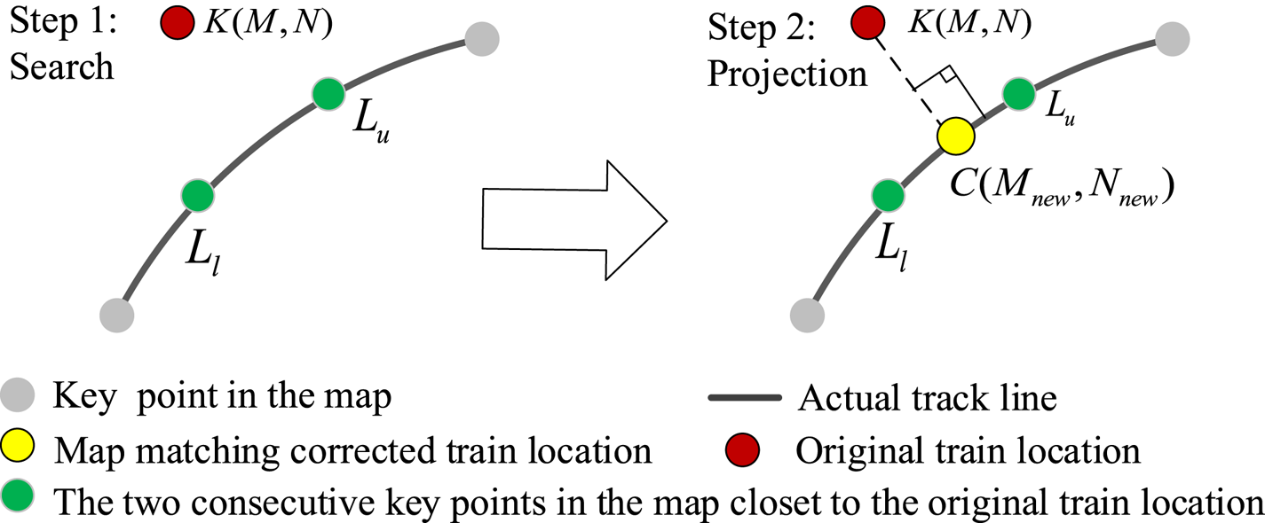
A typical MM application consists of two steps: search and projection, as shown in Figure 1. The first step is to search for the two consecutive key points closest to the original train location from all key points of the map. Due to the close distance between these two consecutive key points, the line segment between the two of them can be approximated as a straight line, called the nearest match interval. Then the original train location is projected perpendicularly on the nearest match interval to obtain a new point. The new point is called the map-matching corrected train location and output as the final train location.
Typical map-matching steps

Different from the traditional MM method with the shortest path search algorithm (Wei et al., Reference Wei, Sirui, Baigen, Jian and Wei2018), the proposed advanced MM-augmented TC GNSS/INS integration method uses a binary search algorithm to quickly search for the nearest interval with less comparison times to improve the operation efficiency. In addition, the original train location is derived from the one-step predicted location not the final estimated location after the measurement update. This altered original train location can avoid poor positioning results due to poor measurement quality caused by GNSS signal blockage. Most important of all, the MM-corrected location further fuses with INS as new measurement to improve estimation accuracy instead of output directly. This proposed method is able to improve positioning accuracy and generate smoother positioning solutions in GNSS partly blocked areas.
3.2.1 Binary search algorithm
In the binary search algorithm, the first step is to determine the upper and lower search index u and l for the original point. As the binary search algorithm begins at both the ends of the DTM, the initial value of the upper search index is set to 1 and the total number of track points. Then, the corresponding points are assumed as ${L_u}\textrm{ }({{M_u},{N_u}} )$ and ${L_l}\textrm{ }({{M_l},{N_l}} )$
 .
Define the original point as $K({M,N} )$ and the distances from point $K({M,N} )$
 to the two current search points as ${d_u}$
 and ${d_l}$
 . The corresponding distance calculation function is:

At the same time, the middle search index is updated by averaging the upper and lower search indexes as:

The upper and lower search indexes are constantly updated by comparing the values of ${d_u}$ and ${d_l}$
 . Assign the value of middle search index to the lower search index if ${d_u}$
 is great than ${d_l}$
 . Otherwise, the value of middle search index is assigned to the upper search index. Then the nearest point ${L_{\textrm{mid}}}\textrm{ }({{M_{\textrm{mid}}},{N_{\textrm{mid}}}} )$
 will be determined if the lower index u is equal or greater than the upper index l. The other nearest point (${L_{\textrm{mid} - 1}}$
 or ${L_{\textrm{mid + }1}}$
 ) is then located, which is the closest point to $K({M,N} )$
 between the left and right points of the nearest point ${L_{\textrm{mid}}}$
 . Based on the two nearest points, the nearest match interval is determined.
3.2.2 Advanced MM measurement-augmented method
The accuracy of the MM depends on the accuracy of the DTM and the original point. The DTM is usually generated by a series of highly precise and consecutive track points. To ensure the MM accuracy, the distance between two adjacent points of the DTM is about 3 meters in this paper. For the traditional MM-aided TC GNSS/INS method, the original point is the TC integration position (final estimated position from UKF measurement step). However, the accuracy of the integration position is heavily degraded in GNSS partly blocked areas, and the traditional MM-aided method is unable to ensure the matching accuracy.
To solve the problem, this research considers MM before the degraded GNSS fusion step, and moves MM forward from the measurement update step to the time update step of the UKF. In the time update step, the one-predicted position can be calculated by one-step predicted position error and the INS-derived position in a short time. Note that the one-step predicted position error position is usually set to zero due to the closed-loop correction in the TC GNSS/INS integration method. Thus, the accuracy of the one-step predicted position mainly depends on the INS-derived position, which performs short-time accuracy. In this paper, the one-step predicted position outputs as an original point for MM and the corresponding matched position is generated via point-line MM. Due to the short-time accuracy of the matched position, it can be taken as a new measurement to fuse with INS to augment TC GNSS/INS instead of direct output in GNSS partly blocked areas. This matched position is defined as an advanced MM measurement.
The one-step predicted point is perpendicularly projected on the nearest match straight to obtain the MM point ${{\bf r}_{\textrm{MM}}}$ . An additional position is updated by fusing n advanced MM position with the INS-derived position in the position domain. Hence, the addition measurement vector is calculated by advanced MM position and INS position difference and is written as:

The additional measurement model can be described as:

where ${{\bf o}_{\textrm{MM}}}(t)$ denotes measurement noise of the MM point and the corresponding covariance matrix is ${{\bf R}_{\textrm{MM}}}$
 ; and ${{\bf H}_{\textrm{MM}}}(t)$
 denotes the measurement matrix and is calculated as:

With the poor GNSS pseudorange rate and pseudorange in GNSS partly blocked areas, the accuracy of integration navigation solutions is decreased. The purpose of this research is to take advantage of available high-precision geographic information on DTM without adding additional sensors. Hence, the new MM position from additional position updates is applied to aid GNSS measurements and enhance the measurement model to maintain system positioning accuracy.
Compared to the standalone UKF-based tightly coupled GNSS/INS integration method, only the measurement vector and measurement model of the advanced MM-enhanced tightly coupled GNSS/INS integration method have changed.
Hence, the system measurement vector of the augmented integration method can be written as:

The new nonlinear measurement model is:

specifically,

Although the MM position model is linear, it is also conducted using 2n + 1 linear computation as with the pseudorange rate measurement model to simplify the system structure.
The corresponding covariance ${{\bf R}_{\textrm{triple}}}$ of the measurement noise ${{\bf o}_{_{\textrm{triple}}}}(t)$
 is up to the GNSS measurement accuracy and DTM accuracy at the same time:

Compared to traditional MM with TC GNSS/INS integration position, the proposed advanced MM measurement-augmented TC GNSS/INS with error-state UKF could, in theory, improve position accuracy in GNSS partly blocked areas. On the one hand, the MM step is carried out in the time update step of the EKF to avoid the poor effect of the degraded GNSS at the current epoch. On the other hand, the matched position as a new measurement to fuse with INS to augment degraded GNSS to generate an accurate position in GNSS partly blocked areas.
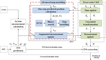
Figure 2 displays the architecture of advanced MM measurement-augmented TC GNSS/INS with error-state UKF. The one-step predicted error state output not only for generating sigma points but also for calculating one-step predicted position. Then the DTM is added to help the binary search algorithm to locate the nearest match interval. Based on the nearest match interval, the matched position is generated via a point-line map-matching method. Together, the augmented position measurement and original measurement serve as the input of UKF with different weight.
The architecture of the proposed advanced MM measurement augmented TC GNSS/INS integration with error-state UKF

4. System design of robust train localisation method
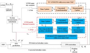
Figure 3 displays the architecture of the robust TC GNSS/INS-based train localisation method with UKF and advanced MM. Note that the robust train localisation method consists of three parts: measurement sensing, navigation mode decision and system filter.
The architecture of the designed robust train localisation method

4.1 Measurement sensing
The GNSS measures the raw pseudorange and pseudorange rate. The IMU measures acceleration and angular velocity to generate the train's position and velocity and is further used to calculate the equivalent pseudorange and pseudorange rate.
4.2 Navigation mode decision-voter
The integration navigation system determines navigation mode using the number of visible satellites. When the train runs in areas where the number of visible satellites is greater than four (defined as GNSS open-sky areas), the system operates in TC GNSS/INS mode with error-state UKF. When the number of visible satellites is fewer than or equal to four and greater than zero (defined as GNSS partly blocked areas), the system switches to advanced MM-augmented TC GNSS/INS mode with error-state UKF. The standalone INS mode is used to provide navigation solutions in GNSS fully blocked areas for a short time. For long tunnels, the MM-augmented INS (INS/MM) mode is used to continue to provide navigation information.
4.3 System filter
Based on this previous decision, the system must estimate the system error state using different system filters.
In TC GNSS/INS mode with error-state UKF, the pseudorange and pseudorange rate difference are input as a measurement. The time updating achieves system error state prediction and corresponding error covariance updating using Equations (11) and (12). Then the UT is used to generate sigma points and associated weights using Equations (13) to (16). The final measurement update is conducted using Equations (19) to (24).
In advanced MM measurement-augmented TC GNSS/INS mode with error-state UKF, the system measurement input includes pseudorange difference, pseudorange rate difference as well as MM position difference. The error-state UKF is still used for the nonlinear estimation.
Based on the different system filters, the proposed robust train localisation method can generate accurate and robust navigation solutions in all environment.
5. Experiment and result analysis
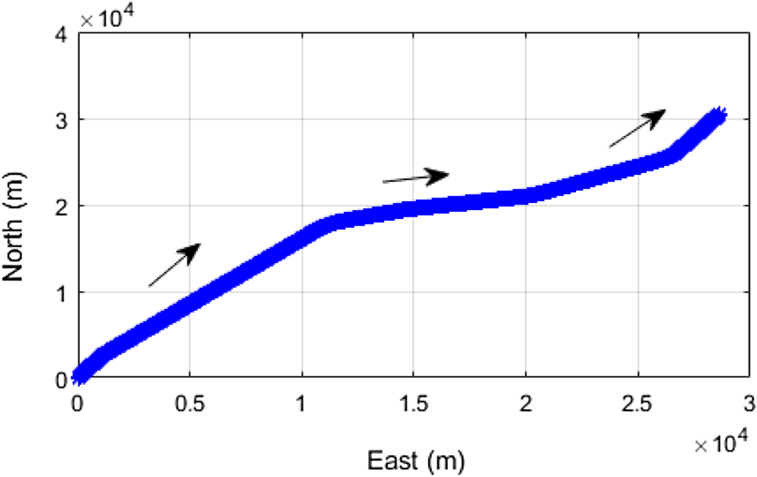
To evaluate the performance of the proposed robust train localisation method, an experiment was carried out on the Qinghai–Tibet railway in China in June 2019. The test time was about 43 minutes and the test trajectory was approximately 43 km. Figure 4 displays the test trajectory.
Testing trajectory

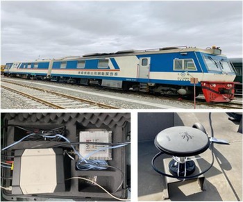
The experimental device was a commercial NovAtel SPAN-FSAS inertial navigation system including an iMAR-FSAS IMU and a NovAtel OEM6 GNSS receiver. The IMU and GNSS receiver was placed inside the cab to collect IMU and GNSS measurements. The GNSS antenna was mounted on the roof of the testing train. The testing train called the rail flaw detection car is shown in the top plot in Figure 5. The lower-left and lower-right plots are NovAtel SPAN-FSAS and GNSS antenna, respectively.
Testing train and experimental device

The output rate of IMU raw measurements and GNSS raw measurements were 200 Hz and 10 Hz, respectively. Note that the raw data were collected and post-processed in the presented methods. At the same time, the system reference was the real-time and high-precision tightly coupled integration solution from the SPAN inertial navigation system.
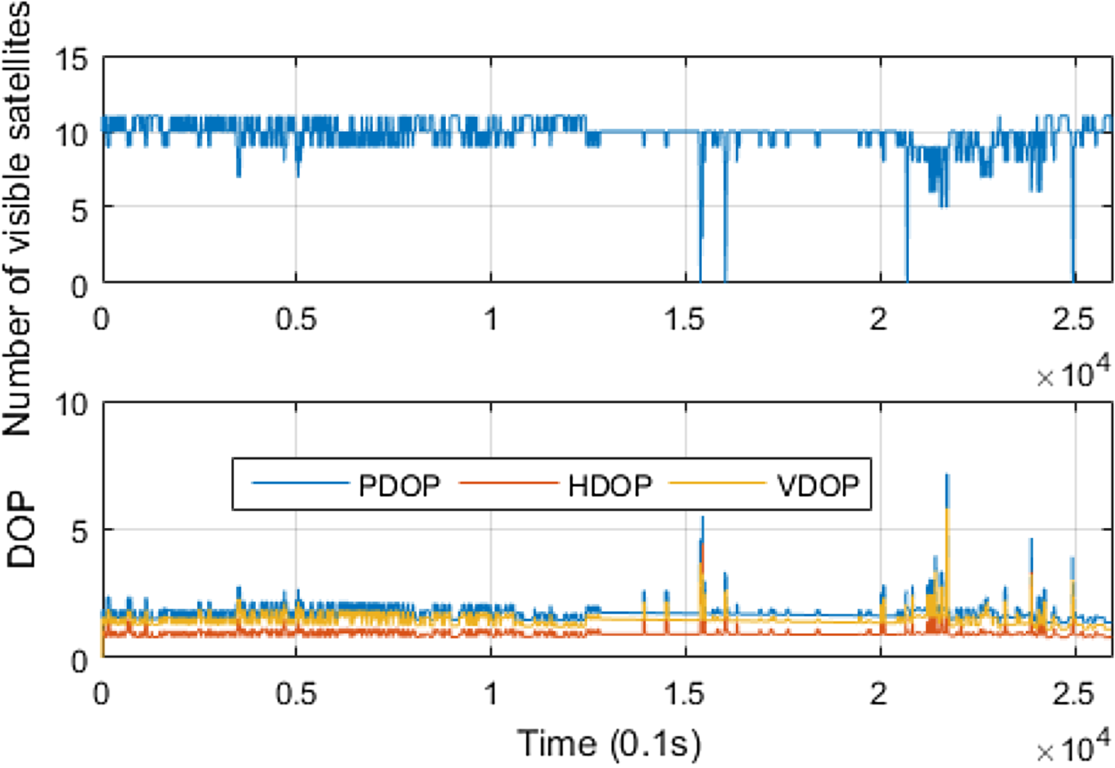
Figure 6 shows both the GNSS visibility and signal geometry during the entire testing period. The GNSS signal geometry change is usually evaluated using the dilution of precision (DOP), which contains position dilution of precision (PDOP), the horizontal dilution of precision (HDOP) and the vertical dilution of precision (VDOP). As shown in Figure 6, more than four satellites were visible during most of the testing periods. In addition, the visible satellites were obviously fewer than four during several short periods, due to momentary GNSS signal occlusion.
GNSS visibility and signal geometry

5.1 Navigation performance evaluation of TC GNSS/INS with error-state UKF
To evaluate the navigation performance of the proposed methods, a brief summary of the three methods mentioned in this paper is conducted as follows.
• Method 1: TC GNSS/INS integration with error-state EKF is abbreviated as EKF GNSS/INS method.
• Method 2: TC GNSS/INS integration with error-state UKF is abbreviated as UKF GNSS/INS method.
• Method 3: Proposed advanced MM measurement-augmented GNSS/INS integration with error-state UKF is abbreviated as UKF GNSS/INS/ Advanced MM method.
• Method 4: Original MM-aided GNSS/INS integration with error-state UKF is abbreviated as UKF GNSS/INS/ Original MM method. Note that the original MM algorithm is detailed in author's previous work (Wei et al., Reference Wei, Sirui, Baigen, Jian and Wei2018).
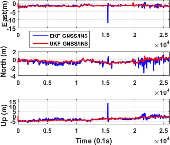
Figure 7 gives the position difference for method 1 and method 2. The overall position difference of method 2 just has a very slight offset to that of method 1 in all directions. Note that the north position difference for method 2 performs especially smaller compared with method 1. That means the method 2 can generate comparably better accuracy than method 1. In addition to the positioning accuracy, it is obvious that the position solution of method 2 is smoother than that of method 1 in all three directions, especially in areas where visible satellites number fewer than four (1537 ⋅ 3 s to1543 ⋅ 1 s) and satellites frequently change (2069 ⋅ 1 s to 2497 ⋅ 5 s). This is because the posterior mean and covariance of the estimated state with higher accuracy are approximated using a set of weighted sigma points in UKF, which results in a better performance than EKF.
Position difference of method 1 and method 2

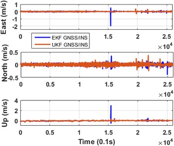
Figure 8 plots the velocity difference of method 1and method 2. Similar to the position result, the velocity result of the two methods are also almost coincide to each other except for two jump points.
Velocity difference of method 1 and method 2

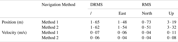
To evaluate the navigation performance of method 2 more accurately, Table 1 lists the commonly used statistical results, including position and velocity difference distance root mean Square (DRMS) and root mean square (RMS) of method 1 and method 2. As detailed in Table 1, the position and velocity DRMS and RMS results are almost consistent with the previous analysis, which verifies that UKF can generate equivalent, perhaps even higher-precision, navigation solutions than EKF.
Position and velocity comparison of EKF and UKF method

5.2 Robustness performance evaluation of proposed method
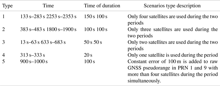
The majority of the test environment in this research is GNSS open-sky area, and contains one short GNSS partly blocked area and four short GNSS fully blocked areas. In fact, the practical operation environments are really complex with more and longer GNSS partly blocked scenarios than in the test environment. Since in the areas with severe signal blockage, multipath problems of satellite signals also occur frequently, both the GNSS partly blocked scenario and pseudorange error should be included in the simulation. To further demonstrate the good robustness of the method in GNSS degraded areas, four types of GNSS partly blocked scenarios and one pseudorange error scenario during eight periods were simulated in the test experiments and are listed in Table 2.
Simulated scenarios description

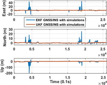
Figure 9 shows the position difference comparison between method 1 and method 2 with five types of simulations. For the GNSS partly blocked areas, it is obvious that the position difference of method 1 is larger than that of the method 2 during the seven simulation periods, especially during the only one visible satellite periods (313 s to 333 s), only three visible satellites periods (383 s–483 s and 1800 s to 1900 s) and only four visible satellites periods (2253 s to 2353 s). In the remaining three simulation scenarios, the position difference of the two system performs a light offset to each other. During the pseudorange error periods, the position difference of method 2 is still significantly better that of method 1. This is because the weighting factor in UKF can reduce the impact of pseudorange error on the navigation results.
Position difference of method 1 and method 2 with five types of simulations

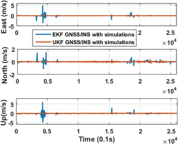
The velocity difference for method 1 and method 2 with five types of simulations are also calculated and shown in Figure 10. A similar conclusion can be drawn that the velocity difference of method 2 is smaller and smoother than that of method 1 during the simulation periods.
Velocity difference of method 1 and method 2 with five types of simulations

This position and velocity comparison analysis further confirms that the UKF has better robustness and accuracy than EKF in both GNSS partly blocked areas and pseudorange error areas.
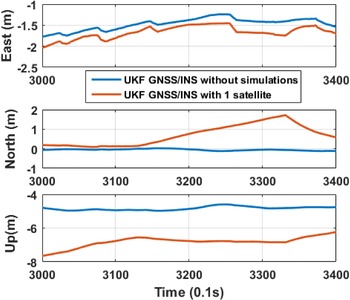
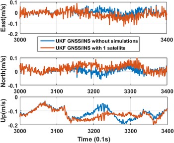
To further observe the robustness of method 2 in GNSS partly blocked areas clearly and concretely, the navigation solutions of method 2 with and without GNSS partly blocked simulations during the seven simulated periods are drawn separately. Due to similar offset tread of method 2 with and without simulations in four simulated scenarios, only one of the typical results in one simulated satellite are analysed in detail, and other results are shown in Appendix A.
Figures 11 and 12 show the position and velocity difference comparison of method 2 with and without one simulated satellite. Note that there is a sight deviation between method 2 with and without one simulated satellite. It is further verified that method 2 can provide robust navigation solutions in GNSS partly blocked environments.
Position difference of method 2 with and without one visible satellite

Velocity difference of method 2 with and without one visible satellite

However, the navigation solution accuracy still has a divergence in different GNSS partly blocked environments and in different navigation directions compared to that in GNSS open-sky environments. Therefore, an advanced map-matching using a binary search algorithm and an additional position update with the DTM is proposed to enhance and optimise navigation performance.
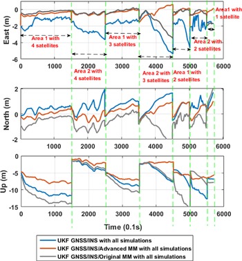
To evaluate the robustness of method 3, the navigation solution comparison of method 2 and method 4 are made. To focus on analysing the robustness only in GNSS partly blocked areas, all the simulated areas are extracted separately and spliced together according to simulation types, as shown in Figure 13. Different simulation scenarios are separated by green dotted lines. The entire simulation time is 570 s.
Comparison of position difference of method 2, method 3 and method 4 in all GNSS partly blocked simulation areas

As shown in Figure 13, the position difference of method 3 in orange, is obviously smaller and smoother than that of method 2 in all three directions in each simulation scenario. It indicates that method 3 can generate better position solutions compared with method 2 in GNSS partly blocked environments. It is because the new MM position measurement generated by advanced map-matching is added to locate with the original GNSS measurements. At the same time, the MM position measurement performs high accuracy and takes up more weight than poor GNSS pseudorange measurement, which is reflected by the corresponding measurement noise covariance matrix.
In addition, the position difference of method 4 is significantly larger than that of method 3 in area 2 with three satellites, but the position difference of both methods is very close to each other in other GNSS partly blocked areas. The north and up position difference of method 4 is larger than that of method 3 in all GNSS partly blocked areas. These results indicate that method 3 can generate better position solutions compared with method 2 in GNSS partly blocked environments. It is because the MM results of advanced MM is not directly output like original MM, but is further integrated with INS as augmented measurement input to weaken the divergence of INS errors.
Hence, the proposed method 3 has superior accuracy and robustness compared with method 2 and method 4 in GNSS partly blocked environments.
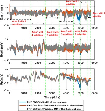
Figure 14 shows the comparison of velocity difference of method 2, method 3 and method 4 in all GNSS partly blocked simulation areas. It can be seen that velocity accuracy of method 3 is improved to a certain extent compared with method 2 and method 4. However, compared to the improvement in position accuracy, the improvement in velocity accuracy is not obvious. The MM position measurement is the main reason for the obvious improvement in positioning accuracy. With the aid of the MM position measurement, the GNSS receiver's antenna position changes, which leads to the line-of-sight vector to change, thereby affecting the final velocity estimation.
Comparison of velocity difference of method 2, method 3 and method 4 in all GNSS partly blocked simulation areas

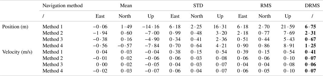
To accurately evaluate positioning accuracy of proposed method 3 in GNSS partly blocked areas, the position and velocity difference DRMS, RMS, mean and standard deviation (STD) of method 2, method 3 and method 4 are summarised in Table 3. The position DRMS and of method 3 is 0 ⋅ 67 m and shows a great improvement of about 71% and 46% compared to that of method 2 in 2 ⋅ 31 m and method 4 in 1 ⋅ 25 m. The up-position RMS also exhibits an improvement of about 29% from 7 ⋅ 69 m in method 2 and about 39% from 8 ⋅ 91 m in method 4 to 5 ⋅ 43 m in method 3.
Difference statistics of four different navigation method with simulations

By comparing the position mean, STD and RMS of the two methods, a similar conclusion is obtained. However, the velocity statistical values of the two methods are almost equal.
Furthermore, the statistical results of method 1 (EKF) in GNSS partly blocked areas are also listed in Table 3. The position and velocity DRMS of method 2 have an obvious improvement of about 66% (from 6 ⋅ 75 m to 2 ⋅ 31 m) and 83% (from 0 ⋅ 41 m/s to 0 ⋅ 07 m/s) compared with those of method 1.
The up position and velocity RMS of method 2 also perform an obvious improvement of about 64% (from 21 ⋅ 59 m to 7 ⋅ 69 m) and 81% (from 0 ⋅ 54 m/s to 0 ⋅ 10 m/s). The results further demonstrate that UKF can provide more accurate and robust navigation solutions than EKF when a train runs in GNSS partly blocked areas.
6. Conclusion and future work
To maintain the positioning accuracy and robustness for TC GNSS/INS integration in GNSS partly blocked areas, an advanced MM measurement-augmented TC GNSS/INS integration method with error-state UKF is proposed. In the proposed method, a binary search algorithm is applied to quickly find the nearest match interval from the DTM to improve search efficiency. Based on the nearest match interval, the matched position of one-step predicted position generated via point-line projection inputs as an augmented measurement to further fuse with INS. The augmented measurement can provide a compensation for degraded GNSS pseudorange in position domain. In GNSS open-sky areas, the TC GNSS/INS integration method with error-state UKF is operated to provide accurate and robust navigation solutions. By combining the two methods, a robust train localisation system is designed to achieve continuous and reliable position information in all environments.
Both the real train test and simulations experiment were conducted. On the one hand, the results confirm that UKF can provide better navigation solutions, especially in GNSS partly blocked areas. On the other hand, the horizontal position of proposed advanced MM measurement-augmented TC GNSS/INS method with UKF can achieve 0 ⋅ 67 m with an improvement of 71% compared with standalone UKF method. The result indicates that the advanced map-matching method could optimise positioning accuracy and system robustness.
In addition, the proposed method in this research aims to aid trackside equipment but not to totally replace them. Due to the slow transition from a ground trackside method to a train-onboard method, some existing railway lines still adopt the ground trackside method to provide position information. When the traditional method fails, the proposed method can be used as an aid or supplement to continue to provide navigation solutions. To ensure the safety requirements of trains, the proposed method can be considered as an aid to the traditional ground trackside method.
In summary, the proposed robust train localisation method based on TC GNSS/INS integration with error-state UKF and advanced MM-augmented measurement can provide superior navigation solutions in all environments in terms of both accuracy and robustness. In addition, the proposed method improves system positioning performance in GNSS degraded areas simply by changing the MM order to generate a new measurement without adding external sensors, which is also low-cost and easy to implement in practical train localisation applications.
The next-step challenges to address include:
• The optimised digital track map not only includes position information, but also related attitude information. The MM-augmented measurements can extend from single position to position/ attitude to further improve system navigation performance, while at the same time balancing navigation performance and cost/efficiency by choosing different-precision maps for different train localisation applications.
• The simple point-line projection method applied in this research is limited for parallel tracks or turnouts due to the positioning accuracy of the original point. The weighted distance from point-line projection and heading can combinate to achieve more accurate matching.
• The Beidou Navigation Satellite System (BDS) built by China (Jun et al., Reference Jun, Xia and Chengeng2020) could be introduced to achieve BDS/GPS multi-constellation-based TC integration. Using only a multi-system GNSS receiver, this method could reduce the risk of single-constellation positioning decrease and failure due to the increased number of visible satellites.
Future research would be focused on robust train integration positioning without adding other sensors via taking full advantage of the existing sensors.
Acknowledgments
The first author would like to thank the China Scholarship Council (CSC) for supporting her visit at the Institute of Communications and Navigation, German Aerospace Center (DLR- Deutsches Zentrum für Luft- und Raumfahrt) in Oberpfaffenhofen, Germany.
Funding statement
This work was supported in part by the Joint Funds of the National Nature Science Foundation of China (Grant number U1934222), National Natural Science Foundation of China (62027809) and National Natural Science Foundation of China (U2268206).
Appendix A
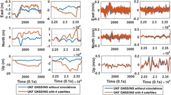
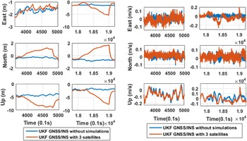
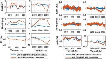
The position and velocity for method 2 with and without simulations in different scenarios are shown as follows.
Position and velocity difference for method with and without four visible satellites

Position and velocity difference for method 2 with and without three visible satellites

Position difference for method 2 with and without two visible satellites