1 Introduction
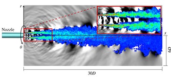
Turbulent jets at high subsonic Mach number are relevant to commercial aircraft noise and have been the subject of recent experiments (Viswanathan Reference Viswanathan2004; Hileman et al. Reference Hileman, Thurow, Caraballo and Samimy2005; Suzuki & Colonius Reference Suzuki and Colonius2006; Cavalieri et al. Reference Cavalieri, Rodríguez, Jordan, Colonius and Gervais2013; Fontaine et al. Reference Fontaine, Elliott, Austin and Freund2015) and large-eddy simulations (Bodony & Lele Reference Bodony and Lele2008; Bogey & Bailly Reference Bogey and Bailly2010; Bogey, Mardsen & Bailly Reference Bogey, Mardsen and Bailly2012; Brès et al. Reference Brès, Jordan, Colonius, Rallic, Jaunet and Lele2014, Reference Brès, Jaunet, Le Rallic, Jordan, Colonius and Lele2015; Lorteau, Cléro & Vuillot Reference Lorteau, Cléro and Vuillot2015). In the simulations of Brès et al. (Reference Brès, Jordan, Colonius, Rallic, Jaunet and Lele2014, Reference Brès, Jaunet, Le Rallic, Jordan, Colonius and Lele2015), for example, waves are clearly visible in the potential core of the jet. Figure 1 shows an instantaneous snapshot of the jet that illustrates this phenomenon. The colour and greyscale contours show the vorticity and pressure fluctuations, respectively, on a planar slice of the jet passing through the polar axis. In addition to the signatures of vortical structures in the shear layer, the pressure field in the potential core clearly contains waves that have a coherent phase and slowly varying wavelength over the first several diameters of the jet. The purpose of this paper is to examine and model these waves. We will show that they are an intrinsic feature of the jet dynamics that can be described by linear instability modes of the jet. In particular, we will show that they are resonating acoustic waves that are trapped within the potential core.
The linear modes of jets have been studied for over fifty years using models with various approximations. Batchelor & Gill (Reference Batchelor and Gill1962) and Lessen, Fox & Zien (Reference Lessen, Fox and Zien1965) investigated the temporal stability of incompressible and compressible jets, respectively, using an inviscid, parallel-flow idealization of the jet in the form of an infinite, cylindrical vortex sheet. In his seminal study, Michalke (Reference Michalke1970) considered the spatial stability of the compressible cylindrical vortex sheet and identified two distinct families of modes: the well-known Kelvin–Helmholtz mode and a second family that he called mode II. Michalke (Reference Michalke1971) went on to show that these same two mode families persist when the finite thickness of the shear layer is taken into account. We will show that the potential-core waves can be modelled using modes from the mode II family.
Tam & Hu (Reference Tam and Hu1989) further investigated models equivalent to Michalke’s and distinguished two subfamilies of mode II based on phase velocity, which they called supersonic and subsonic instability waves. The group velocity of these waves depends on the jet Mach number. Jets with sufficiently high supersonic Mach numbers support both subfamilies, which include both upstream- and downstream-propagating waves. Jets with low subsonic Mach numbers support only upstream-propagating subsonic instability waves. For an intermediate range of Mach numbers that was not considered by Tam & Hu (Reference Tam and Hu1989), we will show that there exist narrow frequency bands for which both upstream- and downstream-propagating waves are supported, while only upstream-propagating waves exist at all other frequencies. This provides one of the necessary ingredients for the trapped waves to resonate. We also show that at certain frequencies the relevant jet instability modes experience the annular shear layer as a duct with a pressure-release surface and are therefore radially confined to the potential core. This motivates our use of the term ‘trapped’ to describe the waves.
Instantaneous snapshot of the jet. Greyscale: pressure fluctuations. Colour: vorticity. The pressure field shows the presence of waves in the potential core of the jet.

Parallel-flow jet models have also been analysed using the spatiotemporal stability theory developed by Briggs (Reference Briggs1964) and Bers (Reference Bers1983) to study the absolute instability that is observed in heated, low-speed jets (Monkewitz & Sohn Reference Monkewitz and Sohn1988; Jendoubi & Strykowski Reference Jendoubi and Strykowski1994; Lesshafft & Huerre Reference Lesshafft and Huerre2007). We will apply the spatiotemporal theory to an isothermal jet to show that the core waves are neutrally stable over a range of streamwise positions.
To partially account for the influence of the slow streamwise variation of the jet, weakly non-parallel models have been developed based on energy methods (Chan Reference Chan1974; Liu Reference Liu1974), asymptomatic analysis (Crighton & Gaster Reference Crighton and Gaster1976; Tam & Morris Reference Tam and Morris1980; Tam & Burton Reference Tam and Burton1984) and parabolized stability equations (Balakumar Reference Balakumar1998; Yen & Messersmith Reference Yen and Messersmith1998; Gudmundsson & Colonius Reference Gudmundsson and Colonius2011; Sinha et al. Reference Sinha, Rodriguez, Brès and Colonius2014). These analyses have all focused on the streamwise evolution of the Kelvin–Helmholtz mode, which forms a coherent wavepacket structure in the jet mixing layer. We will construct a weakly non-parallel model of the potential-core waves based on a Wentzel–Kramers–Brillouin (WKB) approximation of the relevant modes. To our knowledge, this represents the first weakly non-parallel model of waves from the mode II family. We will show that ‘turning points’ of the WKB solutions play an essential role in the resonance of the trapped core waves.
Global linear stability modes that fully account for the spatial variation of the jet have also been computed for low Reynolds number jets (Nichols & Lele Reference Nichols and Lele2011; Garnaud et al. Reference Garnaud, Lesshafft, Schmid and Huerre2013). In a parallel investigation (Schmidt et al. Reference Schmidt, Towne, Colonius, Cavalieri, Jordan and Brès2017), we compute the global modes of the same Mach 0.9 turbulent jet considered in this paper, which provide additional insight into the trapped waves.
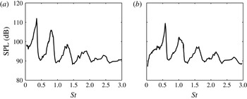
We use an extensive large-eddy simulation (LES) database for a Mach 0.9, isothermal jet to directly observe the trapped acoustic waves and confirm the predictions of the linear theory. In addition, we associate the waves with a series of tones that has previously been observed in experiments using microphones in the near-nozzle region (Suzuki & Colonius Reference Suzuki and Colonius2006; Sinha Reference Sinha2011). An example is reproduced in figure 2. These tones have been observed for only certain combinations of Mach number and temperature ratio and were previously attributed to extrinsic factors such as the presence of debris or an internal resonance in the upstream plumbing. We will show that they are instead generated by the intrinsic resonance of the trapped acoustic waves in the potential core.
Sound pressure level measured by Suzuki & Colonius (Reference Suzuki and Colonius2006) at
 $(x/D,r/D)=(0.35,0.875)$
in a jet with
 $M=U_{j}/a_{\infty }=0.9$
and
 $T_{j}/T_{\infty }=0.84$
: (a)
 $m=0$
; (b)
 $m=1$
. Within the same set of experiments, the substantial peaks seen here were observed at only certain jet operating conditions.

The remainder of the paper is organized as follows. We begin in § 2 by introducing and probing the large-eddy simulation data for the Mach 0.9 isothermal jet that are used throughout the paper to chronicle the fundamental properties of the trapped waves. In § 3, we use three parallel-flow models, along with spatiotemporal stability theory, to investigate the local properties of the trapped waves close to the jet inlet. The weakly non-parallel model is developed in § 4. Mach number and temperature ratio effects are considered in § 5 with the goal of explaining the associated tones that are observed only for certain jet operating conditions. In § 6, we summarize the paper and speculate as to the relevance of the trapped waves to the overall dynamics and acoustics of the jet.
2 Observations from data
In this section, we characterize the waves observed within the potential core and detected outside of the jet in the near-nozzle region. After describing the physical set-up and numerical database that is used throughout the paper, we identify the pertinent waves within the data and examine their traits.
2.1 LES database
We use data from a high-fidelity large-eddy simulation (LES) of a subsonic turbulent jet issued from a round convergent–straight nozzle. The jet is isothermal (
 $T_{j}/T_{\infty }=1.0$
), and the jet Mach number is
 $M_{j}=U_{j}/c_{j}=0.9$
, where
 $U$
is the mean (time-averaged) streamwise velocity,
 $c$
is the speed of sound,
 $T$
is the mean temperature and the subscripts
 $j$
and
 $\infty$
refer to the jet exit and free-stream conditions, respectively. The Reynolds number is
 $Re_{j}=\unicode[STIX]{x1D70C}_{j}U_{j}D/\unicode[STIX]{x1D707}_{j}\approx 1\times 10^{6}$
, where
 $D$
is the nozzle exit diameter.
The simulation was performed using the compressible flow solver ‘Charles’ developed at Cascade Technologies (Brès et al.
Reference Brès, Ham, Nichols and Lele2017), which solves the spatially filtered compressible Navier–Stokes equations on unstructured grids using a finite-volume method. The nozzle geometry is explicitly included in the computational domain and synthetic turbulence boundary conditions are used to trip the boundary layer inside the nozzle. The simulation used approximately sixteen million grid points and was run for a duration of 2000 acoustic time units (
 $tc_{\infty }/D$
). Convergence was demonstrated using a second simulation in which the mesh was refined by a factor of two in each direction. We use data from the baseline simulation (sampled every
 $0.2$
acoustic time units) because of its longer time duration, except for the frequency–wavenumber decomposition described in § 2.5 for which the additional spatial resolution is helpful for resolving high wavenumbers. The accuracy of the LES data was verified via extensive comparisons with measurements taken from a companion experiment conducted at the Bruit & Vent jet noise facility of the PPRIME Institute, Poitiers. Additional details on the simulation and its validation are available in a series of papers by Brès et al. (Reference Brès, Jordan, Colonius, Rallic, Jaunet and Lele2014, Reference Brès, Jaunet, Le Rallic, Jordan, Colonius and Lele2015, Reference Brès, Jaunet, Le Rallic, Jordan, Towne, Schmidt, Colonius, Cavalieri and Lele2016).
2.2 Spectral estimation
Since the jet is stationary in time and periodic in the azimuthal direction, it can be decomposed into Fourier modes of the form
 $$\begin{eqnarray}\boldsymbol{q}(x,r,\unicode[STIX]{x1D703},t)=\mathop{\sum }_{\unicode[STIX]{x1D714}}\mathop{\sum }_{m}\hat{\boldsymbol{q}}_{m,\unicode[STIX]{x1D714}}\text{e}^{\text{i}m\unicode[STIX]{x1D703}}\text{e}^{\text{i}\unicode[STIX]{x1D714}t},\end{eqnarray}$$
where
 $\boldsymbol{q}$
is a vector of flow variables. The ergodic hypothesis permits different temporal segments of the flow data to be regarded as statistically distinct realizations of the jet. For the baseline data, we use segments containing 256 instantaneous snapshots of the jet with 75 % overlap, which provides 154 independent realizations of the jet and a frequency resolution of
 $\unicode[STIX]{x0394}St=\unicode[STIX]{x0394}\unicode[STIX]{x1D714}D/(2\unicode[STIX]{x03C0}U_{jet})=0.0217$
. For the refined data, which have been sampled at a higher rate, we use 1024 snapshots per segment with 75 % overlap to obtain 37 realizations with the same frequency resolution. Estimates of the power spectral density may be computed from these data ensembles as
 $$\begin{eqnarray}\boldsymbol{P}_{m,\unicode[STIX]{x1D714}}(x,r)=\frac{1}{N}\mathop{\sum }_{j=1}^{N}|\hat{\boldsymbol{q}}_{m,\unicode[STIX]{x1D714}}^{(j)}|^{2},\end{eqnarray}$$
where
 $\hat{\boldsymbol{q}}_{m,\unicode[STIX]{x1D714}}^{(j)}$
is the Fourier mode of the
 $j$
th realization of the jet and
 $N$
is the total number of realizations.
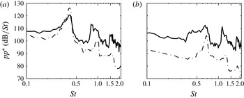
Power spectral density of the of pressure at
 $(x/D,r/D)=(0.02,0.8)$
: (a)
 $m=0$
; (b)
 $m=1$
. Data: (——) Brès et al. (Reference Brès, Jordan, Colonius, Rallic, Jaunet and Lele2014) LES data; (– ⋅ – ⋅ –) experimental measurements.

2.3 Near-nozzle tones
The Mach number and temperature ratio of the present jet are similar to those for which previous authors (Suzuki & Colonius Reference Suzuki and Colonius2006; Sinha Reference Sinha2011) have reported the appearance of discrete spectral tones in pressure measurements taken in the near-nozzle region. These tones exist in the present LES data and also in the companion set of experimental measurements. Figure 3 shows the power spectral density of the
 $m=0$
and 1 components of the pressure signal from both data sets at
 $(x/D,r/D)=(0.02,0.8)$
. The frequency is reported in terms of the Strouhal number
 $St=fD/U_{j}$
. Although some discrepancies exist between the experimental and simulation spectra, both clearly exhibit tones at the same frequencies, which are not harmonic.
2.4 Waves in the potential core
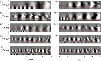
The spatial structure of the pressure field for one realization of the jet at several frequencies is shown in figure 4. Specifically, the real part of the pressure is plotted using linearly distributed contour levels for azimuthal modes 0 and 1 and
 $St=0.39,0.61,0.91,1.21$
and
 $1.52$
. The first, third and fifth frequencies lie within the tonal peaks for
 $m=0$
, while the second and fourth frequencies correspond to tones for
 $m=1$
(see figure 3). In addition to wavepackets associated with the Kelvin–Helmholtz instability in the shear layer (Gudmundsson & Colonius Reference Gudmundsson and Colonius2011), the Fourier modes for
 $St,m$
mode pairs for which tones are observed clearly show the presence of waves within the potential core, while the remaining modes show only weak signs of such waves. This provides a first link between the waves within the potential core and the tones detected outside of the jet.
Fourier components of the LES pressure field. The first and second column are
 $m=0$
and
 $m=1$
, respectively, and the rows, from top to bottom, show
 $St=0.39,0.61,0.91,1.21$
and
 $1.52$
. The contour levels are linearly distributed. The dashed line shows the location where
 $\bar{u}_{x}=0.99U_{j}$
, which serves as a proxy for the outer boundary of the potential core.

Several important properties of these waves can be distinguished from the data. The streamwise wavelength decreases with increasing frequency. The radial shape of the waves follows a regular pattern: at both azimuthal wavenumbers, there is one peak (or anti-node) for the first tonal frequency, two anti-nodes for the second tonal frequency and so on. In all cases, the waves appear to decay rapidly in the radial direction outside of the potential core. The waves are energetic only within the first few diameters of the jet, even though the potential core persists to at least six jet diameters in the streamwise direction.
2.5 Frequency–wavenumber decomposition
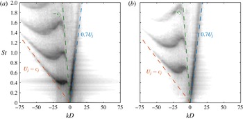
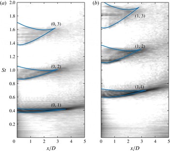
To reveal the spatiotemporal dynamics of these waves, we obtain their empirical dispersion relations by further decomposing the temporally transformed pressure fluctuations into a set of streamwise Fourier modes at fixed radial positions within the potential core. Only the first five jet diameters are included in the Fourier transform to ensure that the results are dominated by the dynamics within the potential core, and we have verified that the results are insensitive to the precise spatial extent and windowing of the transform. This procedure leads to the frequency–wavenumber diagram shown in figure 5. Results are shown for the radial positions
 $r/D=0$
and 0.1 for
 $m=0$
and 1, respectively. Here, iso-contours of the power spectral density of the pressure signal are plotted as a function of the Strouhal number and streamwise wavenumber, which is scaled by the jet diameter. In order to resolve fluctuations occurring at different amplitudes, the scale of the contours is logarithmic and spans five orders of magnitude.
The various bands of energy (the dark regions on the plot) represent a kind of ‘empirical dispersion relation’ for the waves within the potential core. The phase velocity of each wave, scaled by the ambient speed of sound, is
 $v_{p}/c_{\infty }=\unicode[STIX]{x1D714}/k=2\unicode[STIX]{x03C0}MSt/k$
. Therefore, waves in the right and left half-planes have positive and negative phase velocities, respectively. The scaled group velocity is
 $v_{g}/c_{\infty }=\unicode[STIX]{x2202}\unicode[STIX]{x1D714}/\unicode[STIX]{x2202}k=2\unicode[STIX]{x03C0}M\unicode[STIX]{x2202}St/\unicode[STIX]{x2202}k$
and is therefore proportional to the slope of the empirical dispersion relation. Thus, positive and negative slopes represent waves whose energy propagates downstream and upstream, respectively. Locations where the contour line slopes are zero are points of zero group velocity, which play an important role in the theoretical description of the waves developed in §§ 3 and 4.
Frequency–wavenumber decomposition of the pressure in the potential core: (a)
 $m=0$
,
 $r/D=0$
; (b)
 $m=1$
,
 $r/D=0.1$
. The greyscale contours are distributed logarithmically over five orders of magnitude and show the magnitude of the energy, providing an empirical dispersion relation for the waves in the potential core. The lines represent waves with constant group and phase velocities equal to the labelled values.

The properties of the right-most energy band are consistent with Kelvin–Helmholtz instability waves. Its phase and group velocity are positive and nearly equal with a value of approximately
 $0.7U_{j}$
. These waves are vortical and are primarily associated with the dynamics of the shear layer but also have non-zero support in the pressure field within the potential core. In addition to this well-known Kelvin–Helmholtz instability wave, three bands of energy with negative phase velocities can be clearly distinguished for each azimuthal mode (part of a fourth band is visible at the top of the figure for
 $m=0$
). The group velocity of each band is negative for most frequencies and asymptotically approaches the values
 $-c_{j}$
and
 $U_{j}-c_{j}$
at low and high frequencies, respectively. However, for each band there is also a narrow range of frequencies for which their exist waves with both positive and negative group velocities. The waves in these regions are especially energetic, and their frequencies and wavenumbers match those of the waves observed within the potential core and the tones detected just outside the jet.
3 Local models
In this section, we develop a local description of the waves within the potential core of the Mach 0.9 jet using the parallel-flow spatiotemporal linear stability theory developed by Briggs (Reference Briggs1964) and Bers (Reference Bers1983). Although the jet is not a strictly parallel flow, the local theory is applicable due to the slow streamwise variation of the mean flow, compared to the wavelengths of interest, up to the end of the potential core. The local stability theory will be applied to three different models for the jet: the Euler equations linearized about the mean jet, a cylindrical vortex sheet and a cylindrical duct – each of which offers different insights into the potential-core waves.
3.1 Briggs–Bers stability theory
Let the linear one-dimensional partial differential equation
 $$\begin{eqnarray}{\mathcal{D}}\left(-\text{i}\frac{\unicode[STIX]{x2202}}{\unicode[STIX]{x2202}x},\text{i}\frac{\unicode[STIX]{x2202}}{\unicode[STIX]{x2202}t}\right)q(x,t)=s(x,t)\end{eqnarray}$$
represent a parallel-flow model of the jet. The operator does not depend on
 $x$
or
 $t$
. The solution of (3.1) for any source
 $s(x,t)$
, which for the jet could represent incoming fluctuations at the nozzle or volumetric turbulent forcing, can be obtained by convolving the source with a Green’s function
 ${\mathcal{G}}(x,t)$
satisfying
 $$\begin{eqnarray}{\mathcal{D}}\left(-\text{i}\frac{\unicode[STIX]{x2202}}{\unicode[STIX]{x2202}x},\text{i}\frac{\unicode[STIX]{x2202}}{\unicode[STIX]{x2202}t}\right){\mathcal{G}}(x,t)=\unicode[STIX]{x1D6FF}(x)\unicode[STIX]{x1D6FF}(t).\end{eqnarray}$$
Therefore, the dynamics of (3.1) under arbitrary forcing can be determined by analysing the properties of
 ${\mathcal{G}}(x,t)$
.
The Green’s function can be obtained using Fourier and Laplace transforms. Specifically, applying a Fourier transform in
 $x$
and a Laplace transform in
 $t$
to (3.2) gives
 $$\begin{eqnarray}{\mathcal{D}}(k,\unicode[STIX]{x1D714})\hat{{\mathcal{G}}}(k,\unicode[STIX]{x1D714})=1,\end{eqnarray}$$
where
 $k$
and
 $\unicode[STIX]{x1D714}$
are the Fourier and Laplace duals of
 $x$
and
 $t$
, respectively, and
 $\hat{{\mathcal{G}}}(k,\unicode[STIX]{x1D714})$
is the Fourier–Laplace transform of
 ${\mathcal{G}}(x,t)$
. We have ignored initial transients since the jet is statistically stationary. For future use, we define the expression
 $\unicode[STIX]{x1D714}=\unicode[STIX]{x1D714}(k)$
to represent a
 $(k,\unicode[STIX]{x1D714})$
pair that satisfies the dispersion relation
 ${\mathcal{D}}(k,\unicode[STIX]{x1D714})=0$
. Equivalently, the inverse of the expression can be written
 $k=k(\unicode[STIX]{x1D714})$
.
The Green’s function
 ${\mathcal{G}}(x,t)$
is obtained by solving (3.3) for
 $\hat{{\mathcal{G}}}(k,\unicode[STIX]{x1D714})$
and taking the inverse transforms:
 $$\begin{eqnarray}{\mathcal{G}}(x,t)=\frac{1}{4\unicode[STIX]{x03C0}^{2}}\int _{L}\int _{F}\frac{1}{{\mathcal{D}}(k,\unicode[STIX]{x1D714})}\text{e}^{\text{i}(kx-\unicode[STIX]{x1D714}t)}\,\text{d}k\,\text{d}\unicode[STIX]{x1D714}.\end{eqnarray}$$
By the residue theorem, the Green’s function, and thus the general solution of (3.1), is determined by the zeros of the dispersion relation, i.e. the eigenvalues of
 ${\mathcal{D}}$
. In turn, the physical interpretation and significance of these eigenmodes is dictated by their contribution to the Fourier–Laplace integral. Briggs (Reference Briggs1964) and later Bers (Reference Bers1983) performed a detailed analysis of (3.4) that brought to light a number of important concepts that we briefly summarize here.
One important distinction is whether the wave described by an eigenvalue
 $k(\unicode[STIX]{x1D714})$
will contribute to the solution to the right (
 $x>0$
) or left (
 $x<0$
) of the location at which it is excited, i.e. whether it transfers energy downstream or upstream. This question can be addressed by requiring the solution to be causal, which ultimately reduces to a simple criterion based on the asymptotic behaviour of
 $k(\unicode[STIX]{x1D714})$
at large
 $\unicode[STIX]{x1D714}_{i}$
: a mode transfers energy downstream if
 $$\begin{eqnarray}\lim _{\unicode[STIX]{x1D714}_{i}\rightarrow +\infty }k_{i}=+\infty\end{eqnarray}$$
and upstream if
 $$\begin{eqnarray}\lim _{\unicode[STIX]{x1D714}_{i}\rightarrow +\infty }k_{i}=-\infty .\end{eqnarray}$$
The subscripts
 $r$
and
 $i$
refer to the real and imaginary parts of a variable. These two categories of modes are denoted as
 $k^{+}$
and
 $k^{-}$
, respectively.
Two more properties can be distinguished by studying the long-time asymptotic solution of (3.4) along fixed spatiotemporal rays. The first outcome of this analysis is that only eigenmodes that satisfy the condition
 $$\begin{eqnarray}\frac{\unicode[STIX]{x2202}\unicode[STIX]{x1D714}}{\unicode[STIX]{x2202}k}(k^{\ast })=V\end{eqnarray}$$
contribute to the solution along the ray
 $x/t=V$
as
 $t\rightarrow \infty$
. This is a generalization of the standard concept of group velocity and gives a measure of the speed at which the wave propagates. Note that (3.7) implies that
 $\unicode[STIX]{x2202}\unicode[STIX]{x1D714}/\unicode[STIX]{x2202}k$
only takes on this meaning when it is real valued.
Second, the temporal growth rate experienced by a moving observer along the ray
 $x/t=V$
is
 $$\begin{eqnarray}\unicode[STIX]{x1D70E}=\unicode[STIX]{x1D714}_{i}^{\ast }-Vk_{i}^{\ast },\end{eqnarray}$$
where the complex wavenumber
 $k^{\ast }$
satisfies (3.7) and
 $\unicode[STIX]{x1D714}^{\ast }=\unicode[STIX]{x1D714}(k^{\ast })$
. Of particular interest is the so-called absolute growth rate observed at the source location
 $x=0$
, which is determined by the growth rate along the ray
 $x/t=V=0$
, i.e. by waves that do not propagate away from their source. According to (3.8), the absolute growth rate is
 $\unicode[STIX]{x1D70E}^{0}=\unicode[STIX]{x1D714}_{i}^{0}$
, where
 $$\begin{eqnarray}\displaystyle & \displaystyle \frac{\unicode[STIX]{x2202}\unicode[STIX]{x1D714}}{\unicode[STIX]{x2202}k}(k^{0})=0, & \displaystyle\end{eqnarray}$$
 $$\begin{eqnarray}\displaystyle & \displaystyle \unicode[STIX]{x1D714}^{0}=\unicode[STIX]{x1D714}(k^{0}). & \displaystyle\end{eqnarray}$$
 $t$
becomes large. The flow is then said to be absolutely stable. On the other hand, if the absolute growth rate is positive, disturbances grow at their source location and eventually engulf the entire domain – the flow is absolutely unstable. If the absolute growth rate is zero, disturbances neither grow nor decay at their source but instead persist indefinitely – they are neutrally stable. An eigenvalue pair
 $(k^{0},\unicode[STIX]{x1D714}^{0})$
that satisfies (3.9) corresponds to a saddle point in the complex
 $k$
plane formed by the coalescence of two solutions of
 $k=k(\unicode[STIX]{x1D714})$
at
 $k^{0}$
. As emphasized by Bers (Reference Bers1983), a saddle point corresponds to an absolute eigenvalue pair only if formed by one
 $k^{+}$
mode and one
 $k^{-}$
mode.
Finally, the spatiotemporal theory reduces to the classical concepts of temporal and spatial stability when the source is harmonic in space and time, respectively. The spatial theory, in which
 $k(\unicode[STIX]{x1D714})$
is determined for real values of
 $\unicode[STIX]{x1D714}$
, will be particularly relevant to the present investigation. The sign of
 $k_{i}$
governs the growth or decay of the spatial modes –
 $k^{+}$
modes grow in space if
 $k_{i}<0$
and decay if
 $k_{i}>0$
, while the situation is reversed for
 $k^{-}$
modes. Decaying modes represent evanescent waves. Modes with
 $k_{i}=0$
are called propagative waves – they neither grow nor decay as they propagate at their group velocity.
3.2 Linearized Euler equations
We next describe three models for the jet that will be used, in conjunction with the preceding theory, to investigate the potential-core waves and their associated tones. The first model is the Euler equations, linearized about the time-averaged (mean) turbulent jet. The idea here is that large-scale waves, such as those observed in the jet core, experience the mean jet as an ‘equivalent laminar flow’ (Crighton & Gaster Reference Crighton and Gaster1976). This is undoubtedly a caricature of reality (the mean flow never actually exists instantaneously), but has yielded models that achieve compelling agreement with instability waves observed in turbulent jets (Jordan & Colonius Reference Jordan and Colonius2013). Ultimately, the validity of the model will be established ex post facto by its ability to accurately describe the waves observed in the data. We expect viscous effects to play a limited role in the dynamics of the core waves and accordingly neglect them apart from their influence in establishing the mean flow.
If the flow field is represented by a vector of flow variables
 $\boldsymbol{q}$
, then inserting the Reynolds decomposition
 $$\begin{eqnarray}\boldsymbol{q}(x,r,\unicode[STIX]{x1D703},t)=\bar{\boldsymbol{q}}(x,r)+\boldsymbol{q}^{\prime }(x,r,\unicode[STIX]{x1D703},t)\end{eqnarray}$$
into the Euler equations (in cylindrical coordinates) and neglecting terms that are nonlinear in the fluctuation
 $\boldsymbol{q}^{\prime }$
yields the linearized Euler equations:
 $$\begin{eqnarray}\frac{\unicode[STIX]{x2202}\boldsymbol{q}^{\prime }}{\unicode[STIX]{x2202}t}+\unicode[STIX]{x1D63C}_{x}\frac{\unicode[STIX]{x2202}\boldsymbol{q}^{\prime }}{\unicode[STIX]{x2202}x}+\unicode[STIX]{x1D63C}_{r}\frac{\unicode[STIX]{x2202}\boldsymbol{q}^{\prime }}{\unicode[STIX]{x2202}r}+\unicode[STIX]{x1D63C}_{\unicode[STIX]{x1D703}}\frac{\unicode[STIX]{x2202}\boldsymbol{q}^{\prime }}{\unicode[STIX]{x2202}\unicode[STIX]{x1D703}}+\unicode[STIX]{x1D63C}_{0}\boldsymbol{q}^{\prime }=\mathbf{0}.\end{eqnarray}$$
The matrix coefficients are functions of the mean flow
 $\bar{\boldsymbol{q}}$
. The exact form of the Euler equations and resulting matrix coefficients used in this paper are given in appendix A. All variables have been appropriately non-dimensionalized by the ambient sound speed
 $c_{\infty }$
and density
 $\unicode[STIX]{x1D70C}_{\infty }$
and the nozzle diameter
 $D$
.
To apply the local stability theory, we freeze the mean flow at a particular
 $x$
location and, for consistency with the local approximation, neglect streamwise derivatives of the mean flow and the mean radial velocity. In this section we exclusively consider the profile at the inlet (
 $x=0$
); other streamwise positions will be considered in § 4 within the context of a weakly non-parallel extension of the local theory. Taking Fourier–Laplace transforms of the frozen equations, or equivalently applying the normal-mode ansatz
 $$\begin{eqnarray}\boldsymbol{q}^{\prime }(x,r,\unicode[STIX]{x1D703},t)=\hat{\boldsymbol{q}}(r)\text{e}^{(\text{i}kx+\text{i}m\unicode[STIX]{x1D703}-\text{i}\unicode[STIX]{x1D714}t)},\end{eqnarray}$$
yields
 $$\begin{eqnarray}\left[-\text{i}\unicode[STIX]{x1D714}\unicode[STIX]{x1D644}+\text{i}k\unicode[STIX]{x1D63C}_{x}+\unicode[STIX]{x1D63C}_{r}\frac{\unicode[STIX]{x2202}}{\unicode[STIX]{x2202}r}+\text{i}m\unicode[STIX]{x1D63C}_{\unicode[STIX]{x1D703}}+\unicode[STIX]{x1D63C}_{0}\right]\hat{\boldsymbol{q}}(r)=0.\end{eqnarray}$$
Note that
 $m$
is an integer since the azimuthal coordinate is periodic.
Since we wish to identify saddle points in the complex
 $k$
-plane, we will specify (real or complex) values for
 $\unicode[STIX]{x1D714}$
and solve the resulting eigenvalue problem for
 $k=k(\unicode[STIX]{x1D714})$
. The eigenvalue problem is solved numerically by discretizing (3.13) in the radial direction, leading to a matrix eigenvalue problem for
 $k$
. We use fourth-order central finite differences with summation-by-parts boundary closures (Strand Reference Strand1994). Radiation boundary conditions are enforced using a ‘super-grid’ damping layer (Colonius & Ran Reference Colonius and Ran2002) truncated by Thompson (Reference Thompson1987) characteristic conditions, and pole conditions are implemented using the scheme of Mohseni & Colonius (Reference Mohseni and Colonius2000). The eigenvalues and eigenvectors of interest are well resolved and converged using 200 grid points that are non-uniformly distributed to efficiently resolve the shear layer.
3.3 Cylindrical vortex sheet
The second model considered is a compressible, cylindrical vortex sheet, which constitutes an inviscid idealization of the jet – the infinitely thin vortex sheet separates the interior flow from the surrounding quiescent fluid, resulting in a jet with a top-hat profile.
The dispersion relation for this flow was first derived by Lessen et al. (Reference Lessen, Fox and Zien1965) and has been studied by a number of authors (Michalke Reference Michalke1970; Tam Reference Tam1971; Tam & Hu Reference Tam and Hu1989). It can be written schematically as
 $$\begin{eqnarray}{\mathcal{D}}_{j}(k,\unicode[STIX]{x1D714};M,T)=0,\end{eqnarray}$$
with
 $$\begin{eqnarray}{\mathcal{D}}_{j}=\frac{1}{\displaystyle \left(1-\frac{kM}{\unicode[STIX]{x1D714}}\right)^{2}}+\frac{1}{T}\frac{\text{I}_{m}\displaystyle \left(\frac{\unicode[STIX]{x1D6FE}_{i}}{2}\right)\left[\frac{\unicode[STIX]{x1D6FE}_{o}}{2}\text{K}_{m-1}\left(\frac{\unicode[STIX]{x1D6FE}_{o}}{2}\right)+m\text{K}_{m}\left(\frac{\unicode[STIX]{x1D6FE}_{o}}{2}\right)\right]}{\text{K}_{m}\displaystyle \left(\frac{\unicode[STIX]{x1D6FE}_{o}}{2}\right)\left[\frac{\unicode[STIX]{x1D6FE}_{i}}{2}\text{I}_{m-1}\left(\frac{\unicode[STIX]{x1D6FE}_{i}}{2}\right)-m\text{I}_{m}\left(\frac{\unicode[STIX]{x1D6FE}_{i}}{2}\right)\right]}\end{eqnarray}$$
and
 $$\begin{eqnarray}\displaystyle & \displaystyle \unicode[STIX]{x1D6FE}_{i}=\sqrt{k^{2}-\frac{1}{T}(\unicode[STIX]{x1D714}-Mk)^{2}}, & \displaystyle\end{eqnarray}$$
 $$\begin{eqnarray}\displaystyle & \displaystyle \unicode[STIX]{x1D6FE}_{o}=\sqrt{k^{2}-\unicode[STIX]{x1D714}^{2}}. & \displaystyle\end{eqnarray}$$
 $-\unicode[STIX]{x03C0}/2\leqslant \arg (\unicode[STIX]{x1D6FE}_{i,o})<\unicode[STIX]{x03C0}/2$
.
 $\text{I}_{m}$
and
 $\text{K}_{m}$
are modified Bessel functions of the first and second kind, respectively. Again, all quantities have been normalized by the jet diameter and outer thermodynamic quantities such that
 $M=U_{j}/c_{\infty }$
is the acoustic Mach number and
 $T=T_{j}/T_{\infty }$
is the temperature ratio. The jet Mach number is a function of the acoustic Mach number and the temperature ratio:
 $M_{j}=U_{j}/c_{j}=M/\sqrt{T}$
. A short derivation of the dispersion relation is given in appendix B.
Cylindrical vortex-sheet modes are then given by
 $(k,\unicode[STIX]{x1D714})$
pairs that satisfy (3.14). Again, we choose to specify
 $\unicode[STIX]{x1D714}$
and find
 $k$
, which is accomplished using a trust-region-based nonlinear root-finding algorithm (Coleman & Li Reference Coleman and Li1996). Saddle points can be located directly by finding
 $(k,\unicode[STIX]{x1D714})$
pairs that simultaneously satisfy the dispersion relation and the zero-group-velocity condition
 $$\begin{eqnarray}\frac{\unicode[STIX]{x2202}\unicode[STIX]{x1D714}}{\unicode[STIX]{x2202}k}=\frac{\unicode[STIX]{x2202}{\mathcal{D}}_{j}/\unicode[STIX]{x2202}k}{\unicode[STIX]{x2202}{\mathcal{D}}_{j}/\unicode[STIX]{x2202}\unicode[STIX]{x1D714}}=0.\end{eqnarray}$$
The same root-finding method is used to find these points.
3.4 Cylindrical soft duct
The modes of an inviscid cylindrical soft duct (a duct with pressure-release boundary conditions at the wall) will be shown to explain certain aspects of the behaviour of the relevant Euler and vortex-sheet modes and provide insight into the physical mechanisms they describe. The dispersion relation for the soft duct is
 $$\begin{eqnarray}\text{J}_{m}(\unicode[STIX]{x1D6FD})=0,\end{eqnarray}$$
where
 $\text{J}_{m}$
is the Bessel function of the first kind,
 $\unicode[STIX]{x1D6FD}=\text{i}\unicode[STIX]{x1D6FE}_{i}/2$
and
 $\unicode[STIX]{x1D6FE}_{i}$
is given by (3.16a
). A derivation of the dispersion relation is given in appendix C. Equation (3.18) is satisfied for a countably infinite set of
 $\unicode[STIX]{x1D6FD}$
values – the zeros of
 $\text{J}_{m}$
. We denote the
 $n$
th zero of
 $\text{J}_{m}$
as
 $\unicode[STIX]{x1D6FD}_{m,n}$
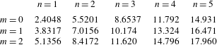
. The first five zeros for
 $m=1$
, 2 and 3 are listed in table 1 for reference. These zeros in turn define a complete set of duct modes.
The
 $n$
th zero of the Bessel function
 $\text{J}_{m}$
, listed to five significant figures.

Starting from the definition
 $\unicode[STIX]{x1D6FD}_{m,n}=\text{i}\unicode[STIX]{x1D6FE}_{i}/2$
, the dispersion relation can be analytically written in the form
 $k=k(\unicode[STIX]{x1D714})$
. There are two roots:
 $$\begin{eqnarray}k_{m,n}^{\pm }=\frac{-\unicode[STIX]{x1D714}M\pm \sqrt{T}\sqrt{\unicode[STIX]{x1D714}^{2}-4(T-M^{2})\unicode[STIX]{x1D6FD}_{m,n}^{2}}}{T-M^{2}}.\end{eqnarray}$$
Using (3.5) and (3.6), the positive and negative roots can be identified as
 $k^{+}$
and
 $k^{-}$
waves, respectively, as denoted by their superscripts. The two roots form a saddle point in the complex
 $k$
plane at
 $$\begin{eqnarray}k_{m,n}^{0}=\frac{-2M}{\sqrt{T-M^{2}}}\unicode[STIX]{x1D6FD}_{m,n},\end{eqnarray}$$
with corresponding absolute frequency
 $$\begin{eqnarray}\unicode[STIX]{x1D714}_{m,n}^{0}=2\sqrt{T-M^{2}}\unicode[STIX]{x1D6FD}_{m,n}.\end{eqnarray}$$
The absolute frequency at each saddle point has zero imaginary part when
 $M^{2}<T$
(which corresponds to
 $M_{j}^{2}<1$
), so the duct modes are neutrally stable in a subsonic flow, as one could anticipate from acoustic theory.
The duct modes approximately satisfy the vortex-sheet dispersion relation in certain situations. Substituting a
 $(k_{m,n}^{\pm },\unicode[STIX]{x1D714})$
combination that satisfies (3.19) into (3.15) gives
 $$\begin{eqnarray}{\mathcal{D}}_{j}(k_{m,n}^{\pm },\unicode[STIX]{x1D714};M,T)=\frac{1}{\displaystyle \left(1-\frac{Mk_{m,n}^{\pm }}{\unicode[STIX]{x1D714}}\right)^{2}}.\end{eqnarray}$$
Therefore, the dispersion relationship
 ${\mathcal{D}}_{j}=0$
is approximately satisfied by the duct mode when
 $$\begin{eqnarray}\left|1-\frac{k_{m,n}^{\pm }M}{\unicode[STIX]{x1D714}}\right|^{2}\gg 1.\end{eqnarray}$$
The parameter
 $1-kM/\unicode[STIX]{x1D714}$
can be expressed as
 $1-M/M_{\unicode[STIX]{x1D719}}$
, where
 $M_{\unicode[STIX]{x1D719}}=\unicode[STIX]{x1D714}/k$
is a Mach number related to the complex-valued phase velocity. Condition (3.23) is satisfied if
 $|M_{\unicode[STIX]{x1D719}}|\ll M$
, i.e. there is a scale separation between the phase velocity and jet velocity. The physical consequence of this condition can be ascertained by considering the vortex-sheet displacement, which arises in the derivation of the vortex-sheet dispersion relation (see appendix B) and can be written as
 $$\begin{eqnarray}\unicode[STIX]{x1D702}=\frac{T}{\unicode[STIX]{x1D714}^{2}\displaystyle \left(1-\frac{M}{M_{\unicode[STIX]{x1D719}}}\right)^{2}}\frac{\text{d}p_{i}}{\text{d}r}\left(\frac{1}{2}\right).\end{eqnarray}$$
Thus, condition (3.23) implies that the vortex-sheet displacement is small for modes that approximately satisfy the soft duct dispersion relation. Furthermore, if
 $|M_{\unicode[STIX]{x1D719}}|\ll M$
we also have
 $|M_{\unicode[STIX]{x1D719}}|\ll 1$
for jets with subsonic acoustic Mach numbers. In this case, the phase velocity of the duct mode is much smaller than the speed of sound, and we have
 $|k|^{2}\gg \unicode[STIX]{x1D714}^{2}$
. In this case, the outer stream only supports evanescent waves with fast radial decay, since
 $\unicode[STIX]{x1D6FE}_{o}$
in (3.16b
) has a large real part and
 $\text{K}_{m}(\unicode[STIX]{x1D6FE}_{o}r)\rightarrow \sqrt{\unicode[STIX]{x03C0}/(2\unicode[STIX]{x1D6FE}_{o}r)}\exp (-\unicode[STIX]{x1D6FE}_{o}r)$
for large
 $|\unicode[STIX]{x1D6FE}_{o}r|$
.
In summary, a soft duct mode satisfying (3.23) is also an approximate solution of the vortex-sheet problem with small vortex-sheet displacement and rapid radial decay in the outer stream – it represents an acoustic wave trapped within the jet core. We will show in the next section that these trapped duct modes are closely related to the waves observed in the potential core of the Mach 0.9 jet.
3.5 Local eigenmodes
The spatiotemporal stability theory outlined in § 3.1 is now applied to each of the three models, with the goal of characterizing the local properties of the waves within the potential core. We begin by examining the eigenmodes of each of the three models at a fixed real frequency. Note that the real part of
 $\unicode[STIX]{x1D714}$
and the Strouhal number are related as
 $St=\unicode[STIX]{x1D714}_{r}/2\unicode[STIX]{x03C0}M$
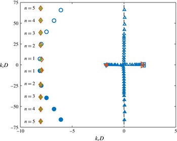
. Figure 6 shows the spatial eigenvalues for each model for
 $m=0$
and
 $St=0.3$
, which serve to introduce the main families of the modes that exist over a wide range of frequencies and azimuthal wavenumbers. Modes from the linearized Euler model that have been identified as spurious, i.e. unphysical artefacts of the numerical discretization, have been omitted from the plot. A number of distinct families of modes can be identified, some of which exist for only a subset of the three models.
The Euler equations and the vortex sheet support a single convectively unstable discrete mode that corresponds to the well-known Kelvin–Helmholtz instability. It is a
 $k^{+}$
mode and has positive phase velocity. The spatial growth rate of the mode is nearly identical for both models, but the vortex-sheet mode has slightly higher phase velocity than its Euler equation counterpart. Since both models are inviscid, the unstable Kelvin–Helmholtz mode also has an evanescent complex-conjugate pair. The Euler equations also support additional convective
 $k^{+}$
modes that describe the neutral transport of vorticity and entropy at the local mean velocity at each radial station. These modes are omitted from the figure to reduce clutter.
Eigenvalues for
 $St=0.3$
and
 $m=0$
. Linearized Euler modes: (▫) Kelvin–Helmholtz; (▵)
 $k^{+}$
free-stream acoustic; (▴)
 $k^{-}$
free-stream acoustic; (▾)
 $k^{-}$
discrete free stream; (○)
 $k^{+}$
duct-like; (●)
 $k^{-}$
duct-like. Vortex-sheet modes: (▹) Kelvin–Helmholtz; (◂)
 $k^{-}$
discrete free stream; (♢)
 $k^{+}$
duct-like; (♦)
 $k^{-}$
duct-like. Duct modes: (
 $+$
)
 $k^{+}$
; (
 $\times$
)
 $k^{-}$
. The dashed lines show the continuous branch of eigenvalues for acoustic waves in an unbounded quiescent fluid.

The Euler equations support two families of modes that represent the discrete approximation of continuous branches of
 $k^{+}$
and
 $k^{-}$
free-stream acoustic modes. These modes have supersonic phase velocity and approximately satisfy the dispersion relation for an acoustic wave in an unbounded quiescent fluid:
 $$\begin{eqnarray}k=\pm \sqrt{\unicode[STIX]{x1D714}^{2}-z^{2}},\end{eqnarray}$$
with
 $z\in [0,\infty ]$
. These branches can be further divided into modes that lie on the real
 $k$
axis, and are therefore propagative, and modes with
 $k_{i}\neq 0$
. The latter modes have positive imaginary part on the
 $k^{+}$
branch and negative imaginary part on the
 $k^{-}$
branch, and are therefore evanescent. The
 $k^{+}$
and
 $k^{-}$
propagative modes together represent acoustic radiation in all directions.
At this frequency, the Euler equations and vortex-sheet model also support a single discrete propagative
 $k^{-}$
mode with negative, subsonic phase velocity that lies near the locus of the
 $k^{-}$
free-stream acoustic branch. For the Euler equations, this mode broke off from the free-stream branch when one of the free-stream modes crossed (below) the sonic point
 $k_{r}=-\unicode[STIX]{x1D714}$
at a critical frequency. Similarly, for the vortex-sheet model, it emanated from a branch point along the branch cut
 $k=-\unicode[STIX]{x1D714}$
. In both cases, then, the locus of this mode represents an acoustic wave that has support both inside and outside of the jet and propagates directly upstream. Accordingly, even though it has subsonic phase velocity and is therefore not a true free-stream acoustic mode, we will call this mode the discrete free-stream acoustic mode to distinguish it from additional discrete acoustic modes that are described next and have significantly less support in the free stream. While both models support only one of these modes at
 $St=0.3$
, more will appear, one at a time, in the same way already described, as the frequency is increased.
Finally, all three models support a number of discrete modes with large negative phase velocities. These modes appear in complex-conjugate pairs, and the modes with
 $k_{i}>0$
and
 $k_{i}<0$
can be shown, using (3.5) and (3.6), to be
 $k^{+}$
and
 $k^{-}$
modes, respectively. They are all therefore evanescent at this frequency, but we will see that each mode pair becomes propagative at certain frequencies. The mode pairs can be classified using two integers,
 $(m,n)$
, where
 $m\in \{0,1,\ldots \}$
is the azimuthal wavenumber and
 $n\in \{1,2,\ldots \}$
is ordered according to
 $|k_{i}|$
, as shown in figure 6. The vortex sheet and duct eigenvalues are nearly identical at this frequency. This is the case because the duct modes satisfy condition (3.23) – their phase velocity
 $\unicode[STIX]{x1D714}/k$
is small compared to the jet velocity, indicating that the duct modes approximately satisfy the vortex-sheet dispersion relation. Equivalently, the vortex-sheet modes nearly satisfy the soft duct dispersion relation – they are duct-like modes. The equivalent Euler eigenvalues are well approximated by the duct and duct-like vortex-sheet eigenvalues for low values of
 $n$
, but diverge for higher values of
 $n$
, a fact that can that can be attributed to the finite thickness of the shear layer. The higher modes, however, are highly damped at this frequency. As mentioned already, each mode pair will become propagative at some frequency, at which point the discrepancy becomes small for every
 $n$
. Therefore, the Euler modes can also be viewed as duct-like. The close correspondence of the vortex-sheet and Euler modes to the duct modes indicates that they represent acoustic waves that experience the jet as a soft duct. Recalling that the waves observed in the potential core had negative phase velocities, these are the modes, along with the discrete free-stream mode, that we will study in detail throughout the remainder of this paper.
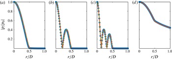
Pressure eigenfunctions at
 $m=0$
,
 $St=0.3$
for (a–c)
 $n=1,2,3$
duct (or duct-like) modes and (d) discrete free-stream mode: (●, blue) linearized Euler; (——, orange) vortex sheet; (– – –, green) soft duct. Note that the duct model does not support the free-stream mode.

The pressure component of the eigenfunction of the first three duct-like modes for all three models is shown in figure 7(a–c). These eigenfunctions exhibit two noteworthy features. First, it is apparent that
 $n$
plays the role of a radial wavenumber, equal to the number of radial anti-nodes in the pressure distribution. Second, the pressure falls off rapidly outside of the jet core for the vortex-sheet and Euler modes (it is zero for the duct modes). In other words, the modes are radially confined, or trapped, in the potential core. This was predicted analytically for the vortex-sheet modes in § 3.4, and is here shown to be true also for the Euler modes. In contrast, the discrete free-stream modes decay much more slowly in the radial direction, as shown in figure 7(d). The eigenfunctions for other azimuthal modes are qualitatively similar, except that the pressure necessarily goes to zero at the polar axis.
We will see that the duct-like and discrete free-stream modes in the vortex-sheet and Euler models, as well as the duct modes, interact with one another in a number of important ways. To be concise, we will use the term core modes to refer to these different modes together as a group.
We next study the behaviour of the core modes as a function of frequency. In particular, we apply the local spatiotemporal theory outlined in § 3.1. To do so, we map lines of varying
 $\unicode[STIX]{x1D714}_{r}$
and constant
 $\unicode[STIX]{x1D714}_{i}$
into the complex
 $k$
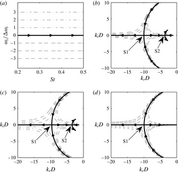
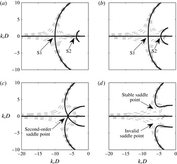
-plane. This is depicted in figure 8, which shows the image of the mapping for the
 $(0,1)$
core-mode group. Focus first on the solid line, which corresponds to
 $\unicode[STIX]{x1D714}_{i}$
= 0. The arrows show the direction of increasing
 $\unicode[STIX]{x1D714}_{r}$
. For all three models, the duct or duct-like eigenvalues start with non-zero imaginary part for low
 $\unicode[STIX]{x1D714}_{r}$
, as shown previously in figure 6, and move toward the real axis as
 $\unicode[STIX]{x1D714}_{r}$
is increased. At a critical frequency, the
 $k^{+}$
and
 $k^{-}$
eigenvalues coalesce. Beyond this frequency, they move along the
 $k_{r}$
axis. The eigenvalue moving toward
 $k_{r}=0$
is a
 $k^{+}$
mode, while the eigenvalue moving away from
 $k_{r}=0$
is a
 $k^{-}$
mode. As
 $\unicode[STIX]{x1D714}_{r}$
is further increased, the
 $k^{+}$
modes in the Euler and vortex-sheet models coalesce with the discrete
 $k^{-}$
free-stream mode, which moves along the real axis away from the origin. Both modes move off the
 $k_{r}$
axis beyond this second critical frequency. In contrast, the second critical point does not exist in the duct model; the
 $k^{+}$
duct mode continuous to move along the real axis toward the origin. The lines with
 $\unicode[STIX]{x1D714}_{i}\neq 0$
make it clear that the two mode intersection points are in fact saddles points, which will hereafter be denoted as S1 and S2, respectively.
The break in the behaviour of the vortex-sheet duct-like modes from that of the duct modes is explained by (3.23). As the modes move toward the origin, their phase velocities increase, so the duct modes less accurately satisfy the vortex-sheet dispersion relation. Eventually, the duct analogy fails, and the two sets of modes diverge. Specifically, since the second saddle is formed between the duct-like mode and a discrete free-stream mode, it represents communication between the acoustic waves in the jet core and the free stream.
Qualitatively equivalent behaviour is observed for other
 $(m,n)$
combinations, most importantly the appearance of two neutrally stable saddle points for the Euler and vortex-sheet models and one neutrally stable saddle for the duct model. The
 $(k^{0},\unicode[STIX]{x1D714}^{0})$
values of each saddle are different for each
 $(m,n)$
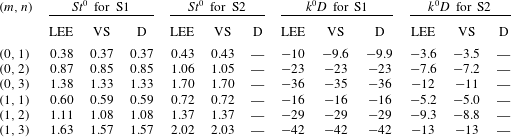
mode group and are reported in table 2 for
 $m=0$
and 1 and
 $n\leqslant 3$
. The values increase monotonically with
 $n$
for a fixed
 $m$
and with
 $m$
for a fixed
 $n$
, a property consistent with the Bessel function zeros,
 $\unicode[STIX]{x1D6FD}_{m,n}$
.
Saddle-point mappings: (a) lines of constant
 $\unicode[STIX]{x1D714}_{i}$
, mapped into the
 $k$
-plane by the (0,1) mode group for (b) the linearized Euler equations, (c) the vortex sheet and (d) the soft duct. The Euler and vortex-sheet mappings contain two saddle points, while the duct mapping has only the first of the two saddle points. The arrows show the direction of increasing
 $\unicode[STIX]{x1D714}_{r}$
. The line types correspond to: (——)
 $\unicode[STIX]{x1D714}_{i}=0$
; (– – –)
 $\unicode[STIX]{x1D714}_{i}<0$
; (– ⋅ – ⋅ –)
 $\unicode[STIX]{x1D714}_{i}>0$
. The lines in the
 $\unicode[STIX]{x1D714}$
-plane have a spacing of
 $\unicode[STIX]{x0394}\unicode[STIX]{x1D714}_{i}=0.015$
.

Absolute wavenumber and frequency values
 $(k^{0},St^{0})$
for the S1 and S2 saddle points for the linearized Euler equations (LEE), vortex sheet (VS) and the soft duct (D) for core-mode group
 $(m,n)$
. Note that the duct model does not contain S2.
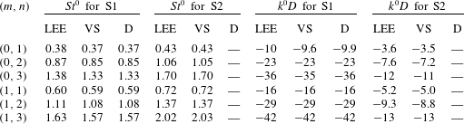
In all cases, the saddle points are formed by a
 $k^{+}$
mode and a
 $k^{-}$
mode and therefore define an absolute frequency–wavenumber pair as described in § 3.1. Since they occur for
 $\unicode[STIX]{x1D714}_{i}=0$
, they correspond to neutrally stable solutions. That is, within a purely linear, inviscid, parallel flow they would neither grow nor decay in time, but rather persist indefinitely.
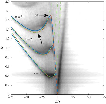
Comparison between modelled and empirical dispersion relations for the
 $m=0$
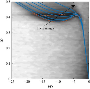
potential-core waves: (——, blue) linearized Euler model; (– – –, orange) vortex-sheet model; (– ⋅ – ⋅ –, green) duct model. The contours show the empirical dispersion relation, as described in § 2.5.

The two saddle points also define so-called ‘cut-on’ and ‘cut-off’ frequencies. At the frequency corresponding to the first saddle point, the two initially evanescent modes become propagative, i.e. they are cut-on. At the frequency corresponding to the second saddle point, two of the modes once more become evanescent – they are cut-off.
3.6 Comparison of local models with data
A useful way to visualize the propagative waves and to compare them to the waves observed in the LES data is to examine their dispersion relation in frequency–wavenumber space. For each model, the first three radial mode groups for
 $m=0$
are plotted in figure 9 on top of the previously discussed frequency–wavenumber spectra of the centreline LES pressure fluctuations. The dispersion relations for the three radial modes are qualitatively similar (as are those for other azimuthal modes). For each dispersion relation, below the frequency of the first saddle point, there exists a single
 $k^{-}$
wave for the Euler and vortex-sheet models with a (negative) group velocity approximately equal to the speed of sound. This is the discrete free-stream mode. There are no propagative duct modes at these frequencies. Note that these curves have been extended to frequencies below their branch point along the path of their locus
 $k=-\unicode[STIX]{x1D714}$
. As the frequency increases, two waves are cut-on in each model – one
 $k^{+}$
mode and one
 $k^{-}$
mode – at a point of zero group velocity. These waves are the propagative duct (or duct-like) modes, and the zero-group-velocity point exactly corresponds to the S1 saddle point. At the second point of zero group velocity, which corresponds to the S2 saddle point, the
 $k^{+}$
duct (or duct-like) wave and the
 $k^{-}$
discrete free-stream mode are cut-off, leaving a single
 $k^{-}$
propagative wave – the
 $k_{-}$
duct (or duct-like) mode. The dispersion relations from the Euler and vortex-sheet models approximate the corresponding empirical dispersion relation extracted from the LES data with striking accuracy, and the duct dispersion relation is a good approximation for wavenumbers to the left of the S2 saddle point. This match gives a first indication that the core modes represent the essential physics of the waves observed within the potential core.
Within the dispersion relation for each mode group, the waves in the LES data are especially energetic at frequencies between the two saddle points. A defining feature of the dispersion relations at these frequencies is the presence of both
 $k_{-}$
and
 $k_{+}$
propagative waves. Each dispersion relation contains only a single
 $k^{-}$
propagative mode at all other frequencies. That is, for each radial mode group, there is a restricted frequency range, bounded by the two saddle points, for which there exist both
 $k^{+}$
and
 $k^{-}$
propagative core modes. We will see in the next section that this provides a necessary ingredient for resonance in the potential core at these frequencies. For now, we simply observe that these frequency ranges accurately predict the tonal peaks observed outside of the jet. For example, the shaded regions in figure 10 indicate the range of frequencies between the two vortex-sheet saddle points for the first three radial mode groups at
 $m=0$
and
 $1$
. These frequency bands, which are almost identical for the Euler model (see table 2) provide an accurate prediction of the tonal frequencies detected in the experimental and numerical near-nozzle pressure field. The duct saddle point gives a good approximation of the lower limit of each frequency band.
Power spectral density of the pressure in the near-nozzle region (
 $(x/D,r/D)=(0.02,0.8)$
): (a)
 $m=0$
; (b)
 $m=1$
. Data: (——) Brès et al. (Reference Brès, Jordan, Colonius, Rallic, Jaunet and Lele2014) LES data; (– ⋅ – ⋅ –) experimental measurements. Model predictions: (


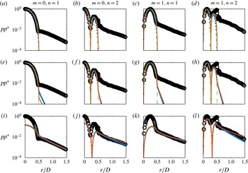
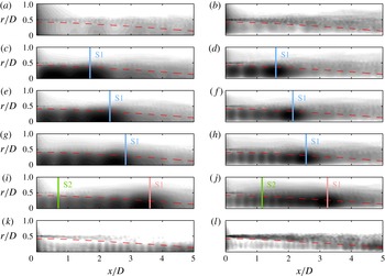
We conclude this section by comparing the radial structure of the core modes to the LES data. In anticipation of the key role of the aforementioned resonance, we make these comparisons for each
 $(m,n)$
mode group at a frequency between the two saddle points. Each column in figure 11 makes this comparison for one mode group. The rows, from top to bottom, show model predictions for the
 $k^{-}$
and
 $k^{+}$
duct (or duct-like modes) and the discrete free-stream mode. For each case, the squared magnitude of the pressure component of the eigenfunction from each model is compared to the power spectral density of the LES pressure fluctuation at the jet inlet (the data are the same in each row). The data and eigenfunctions have been normalized to have a maximum value of one, except in the bottom row where the eigenfunctions have been scaled to visually match the data outside of the potential core.
Within the potential core (
 $r/D<1/2$
), the
 $k^{+}$
and
 $k^{-}$
duct (or duct-like) modes for the three models are indistinguishable from one another, and also closely match the LES data. Outside of the potential core, the data fall off at a rate that is much slower than the duct modes, but that is accurately captured by the discrete free-stream mode. The shape of the free-stream mode is similar to that of the duct modes within the core. Therefore, a linear combination of the duct-like modes and the free-stream mode can account for the radial shape of the power spectral density of the LES data at
 $x=0$
both inside and outside of the potential core. To properly match the data, the free-stream wave is set to be about an order-of-magnitude less energetic than the duct-like modes.
Radial form of the power spectral density of the pressure: (○) LES data at
 $x/D=0$
; (
 $\cdots \cdots$
, blue) linearized Euler model; (——, orange) vortex-sheet model; (– – –, green) duct model. (a–l)
 $m=0$
,
 $St=0.4$
;
 $m=0$
,
 $St=0.96$
;
 $m=1$
,
 $St=0.66$
;
 $m=1$
,
 $St=1.30$
. (a–l) the
 $k^{-}$
and
 $k^{+}$
duct (or duct-like) modes and the discrete free-stream mode. The LES data are the same in each row.

4 Weakly non-parallel model
The underlying assumption of the models developed in the previous section was that the jet can be approximated as an infinite parallel flow. In this section, we pursue a model for the potential-core waves that accounts for two additional effects: the streamwise spreading of the jet and the presence of the nozzle. Specifically, we use a weakly non-parallel extension of the previous parallel-flow spatiotemporal theory based on a WKB ansatz of the form
 $$\begin{eqnarray}q(x,t)\sim A(X)\exp \left[\frac{\text{i}}{\unicode[STIX]{x1D716}}\int _{0}^{X}k(\unicode[STIX]{x1D714};X)\,\text{d}X-\text{i}\unicode[STIX]{x1D714}t\right].\end{eqnarray}$$
Here,
 $\unicode[STIX]{x1D716}$
is a small parameter that typifies the slow streamwise variation of the flow,
 $X=\unicode[STIX]{x1D716}x$
is the slow streamwise variable and
 $A(X)$
is an unknown amplitude function. After some analysis, the complex wavenumber
 $k(\unicode[STIX]{x1D714},X)$
is found to be the solution of a local dispersion relation
 $$\begin{eqnarray}{\mathcal{D}}(k,\unicode[STIX]{x1D714};X)=0\end{eqnarray}$$
obtained by freezing the coefficients of the slowly varying equations at a given
 $x$
and neglecting streamwise derivatives of the mean flow as well as the mean transverse velocity (Bender & Orszag Reference Bender and Orszag1999). Therefore, to first order, the flow dynamics is governed by its local stability properties, which can be analysed using the parallel-flow Briggs–Bers analysis (Huerre & Monkewitz Reference Huerre and Monkewitz1990; Huerre Reference Huerre, Batchelor, Moffatt and Worster2002). We will apply this weakly non-parallel theory to the Euler equations linearized about the spatially evolving mean jet, and in particular to the core modes identified in the previous section. Note that the wavelengths of interest are small compared to the length of the potential core (the longest waves are less than one third of the potential-core length), so the weakly non-parallel model is expected to provide a good approximation of the global behaviour of the potential-core waves.
4.1 Local eigenmodes as a function of streamwise position
The local spatiotemporal properties of the core modes at the jet inlet (
 $x=0$
) were studied in § 3.5 by mapping lines of constant
 $\unicode[STIX]{x1D714}_{i}$
and varying
 $\unicode[STIX]{x1D714}_{r}$
into the complex
 $k$
-plane via the dispersion relation
 ${\mathcal{D}}(k,\unicode[STIX]{x1D714};X=0)=0$
. This analysis is now repeated for other streamwise positions. The image of the mapping for the
 $(0,1)$
mode group is shown in figure 12 for four streamwise locations. As
 $x$
increases, the two saddle points that were identified at
 $x=0$
slowly deform and move towards each other along the
 $k_{r}$
-axis. The absolute frequency remains real valued for both saddle points. They continue this trajectory until they coalesce at
 $x/D=3.62$
, forming a second-order saddle point. Beyond this critical
 $x$
location, both saddle points move off the
 $k_{r}$
-axis and the associated absolute frequency becomes complex valued. The upper saddle point occurs for
 $w_{i}<0$
and is therefore absolutely stable. The lower saddle point occurs for
 $w_{i}>0$
, but both participating modes can be shown to be
 $k^{-}$
modes, making the saddle point irrelevant, as discussed in § 3.1. Therefore, the
 $(0,1)$
core modes are absolutely neutral for
 $x\leqslant 3.62$
and absolutely stable for
 $x>3.62$
.
Saddle points of the LES mean flow at
 $m=0$
and (a)
 $x=0$
, (b)
 $x=3$
, (c)
 $x=3.62$
and (d)
 $x=4$
. The line types correspond to: (——)
 $\unicode[STIX]{x1D714}_{i}=0$
; (– – –)
 $\unicode[STIX]{x1D714}_{i}<0$
; (– ⋅ – ⋅ –)
 $\unicode[STIX]{x1D714}_{i}>0$
. The two saddle points that occur on the real axis for low
 $x$
merge at
 $x=3.62$
and subsequently move off of the real axis.

Dispersion relations for the
 $(0,1)$
mode group: (——) local Euler model at
 $x=0,2,3,3.62,4$
; greyscale contours show the empirical dispersion relation from the LES data. The region outlined by (– – –) shows frequency–wavenumber combinations for which there exist both
 $k^{-}$
and
 $k^{+}$
propagative core waves at some
 $x$
.

The deformation of the image of the
 $k=k(\unicode[STIX]{x1D714};X)$
mapping with streamwise location has a profound impact on the properties of the propagative core waves that are locally supported by the jet. Figure 13 shows the dispersion relations of the
 $(0,1)$
propagative waves at several streamwise locations. As discussed previously, the dispersion relation at
 $x=0$
has two points of zero group velocity, which correspond to the two saddle points and bound a limited range of frequencies for which there exists both
 $k^{-}$
and
 $k^{+}$
propagative waves. As
 $x$
increases, the
 $k_{r}$
separation between the saddle points decreases (cf. figure 12), as does the frequency difference. This results in a progressively narrower frequency range for which the jet supports both
 $k^{-}$
and
 $k^{+}$
propagative trapped waves. At the streamwise location where the two saddles merge, there is a single point of zero group velocity. The saddle points subsequently move off of the real axis, leaving no points of zero group velocity in the dispersion relation for the propagative waves. Since the dispersion curve begins with negative group velocity at low frequencies, and a switch from negative to positive group velocity requires a point of zero group velocity, only
 $k^{-}$
propagative waves remain beyond the streamwise location at which the two saddles coalesce; all
 $k^{+}$
waves are evanescent. We’ll see shortly that this has important implications for the dynamics of the core waves. The outlined region in figure 13 delineates frequency–wavenumber combinations for which there exist both
 $k^{-}$
and
 $k^{+}$
propagative core waves at some
 $x$
. This approximately bounds the high-energy region in the frequency–wavenumber decomposition of the LES pressure data.
Similar behaviour is observed for other
 $(m,n)$
mode groups, but the absolute frequencies and wavenumbers associated with the saddle points are different, as are the critical
 $x$
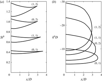
values at which they coalesce and become absolutely stable. Figure 14 gives the frequency and wavenumber values of the two saddle points as a function of
 $x$
for several
 $(m,n)$
mode groups up until the critical merger point. For both
 $St^{0}$
and
 $k^{0}$
, there are two lines for each
 $(m,n)$
that correspond to the two saddle points. These lines necessarily intersect at the streamwise location at which the two saddle points coalesce. Recall that, at each
 $x$
, the two saddle points bound the frequencies and wavenumbers for which both
 $k^{-}$
and
 $k^{+}$
propagative waves exist. Therefore, for each
 $(m,n)$
, both
 $k^{-}$
and
 $k^{+}$
propagative waves exist only for frequencies and wavenumbers on the interior of the region bounded by the
 $St^{0}(x)$
and
 $k^{0}(x)$
curves, respectively, and the line
 $x=0$
. Outside of this region, the
 $k^{+}$
duct-like mode and the
 $k^{-}$
mode that had formed the saddle are cut off.
The (a) frequency and (b) wavenumber position of the two saddle points as a function of
 $x$
up until the merger point for several
 $(m,n)$
mode groups.

4.2 Turning points
In the WKB ansatz (4.1), the streamwise-varying local modes,
 $k(\unicode[STIX]{x1D714};X)$
, are stitched together by the amplitude function
 $A(X)$
to form an approximate global solution at a given frequency
 $\unicode[STIX]{x1D714}$
. The amplitude function, which is determined by a solvability condition at
 $O(\unicode[STIX]{x1D716})$
, becomes singular at so-called turning points of the WKB approximation (Bender & Orszag Reference Bender and Orszag1999). These singularities occur at locations of zero group velocity, which again correspond to saddle points in the complex
 $k$
-plane. These turning points represent special locations in the complex
 $(k,\unicode[STIX]{x1D714},X)$
space at which
 $k^{+}$
and
 $k^{-}$
solutions of the local dispersion relation can exchange energy. Specifically, the
 $k^{+}$
and
 $k^{-}$
modes that coalesce to form the saddle point can be connected at the singularity using a modified ‘inner’ solution that is valid in the vicinity of the turning point (Bender & Orszag Reference Bender and Orszag1999). Therefore, the streamwise-varying saddle points computed in the previous section not only govern the stability properties of the flow, but also represent a mechanism by which
 $k^{+}$
and
 $k^{-}$
core waves can interact.
Before applying these ideas to the jet core modes, it is helpful to first consider them in a simplified context. The WKB solution for acoustic waves within a hard-walled duct with a slowly varying cross-section, and in particular the behaviour of its turning points, has recently been studied by Rienstra (Reference Rienstra2000, Reference Rienstra2003). The duct modes have turning points at the frequencies
 $$\begin{eqnarray}\unicode[STIX]{x1D714}_{m,n}^{0}=\sqrt{1-M^{2}}\unicode[STIX]{x1D6FD}_{m,n}^{\prime }/R(X),\end{eqnarray}$$
where
 $\unicode[STIX]{x1D6FD}_{m,n}^{\prime }$
are the zeros of
 $\text{J}_{m}^{\prime }$
(the derivatives of the Bessel functions) and
 $R(X)$
is the spatially varying duct radius. These saddle points constitute a cut-on/cut-off transition between propagative and evanescent waves, just as they did for the soft duct modes previously discussed in § 3.4. For the infinite duct with constant cross-section, a mode at a given frequency was always either cut-on or cut-off. In contrast, a propagative mode of the spatially varying duct at frequency
 $\unicode[STIX]{x1D714}$
can be cut-off, i.e. become evanescent, due to the changing cross-section at the streamwise location
 $x_{t}$
for which
 $\unicode[STIX]{x1D714}=\unicode[STIX]{x1D714}_{m,n}^{0}(x_{t})$
. At this turning point, an incident
 $k^{+}$
propagative wave is split into a reflected
 $k^{-}$
wave that is propagative (cut-on) and a transmitted
 $k^{+}$
wave that is evanescent (cut-off). The magnitudes and phases of these waves, relative to the incident wave, are described by reflection and transmission coefficients that are determined by matching the outer solutions on either side of the turning point with the appropriate inner solution. The reflection and transmission coefficients are
 $i$
and
 $1$
, respectively.
The situation is quite similar for the jet core modes. A turning point is encountered at
 $x=x_{t}$
by a wave in the
 $(m,n)$
mode group if its Strouhal number satisfies the condition
 $St=St^{0}(x_{t})$
for one of the two
 $(m,n)$
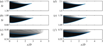
saddle points. This condition can be conveniently visualized by drawing a horizontal line at the desired frequency in figure 14(a). A turning point exists at that frequency for mode group
 $(m,n)$
if the horizontal line intersects one of the
 $St^{0}$
curves for that mode group, and the streamwise location of the turning point is given by the
 $x$
value of the intersection point. If the line does not intersect one of the
 $St^{0}$
curves, then no turning point exists at that frequency. It is interesting to note that the turning points occur well before the end of the potential core at
 $x/D\approx 6$
. By analogy with the spatially varying duct, the turning points are presumably caused by the slow narrowing of the potential core.
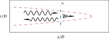
Schematic representation of the behaviour of a
 $k^{+}$
propagative duct-like mode that encounters a turning point at
 $x=x_{t}$
. It is reflected as a
 $k^{-}$
propagative wave and transmitted as an evanescent
 $k^{+}$
wave.

An incident core wave that encounters a turning point is partially reflected and partially transmitted. Since the saddle points represent a cut-on/cut-off transition, an incident wave that is propagative is split into a reflected wave that is propagative and a transmitted wave that is evanescent. For example, the case in which a propagative
 $k^{+}$
core wave encounters a turning point is shown schematically in figure 15. Conversely, an incident wave that is evanescent is split into a reflected wave that is evanescent and a transmitted wave that is propagative. This latter scenario is physically relevant only if the decay rate of the incident evanescent wave is small. An evanescent wave decays exponentially as it travels toward the turning point, leaving little energy to be transmitted to the propagative wave if the decay rate is significant.
The identities of the incident, reflected, and transmitted waves that interact at a given turning point are determined by the modes that coalesce to form the saddle point. Therefore, the participating modes are different for turning points on the upper and lower
 $St^{0}$
curves, which correspond to the S1 and S2 saddle points, respectively. The S1 saddle points are formed between
 $k^{+}$
and
 $k^{-}$
duct-like modes, and therefore provide a mechanism by which
 $k^{+}$
duct-like modes can be converted into
 $k^{-}$
duct-like modes, and vice versa. The S2 saddle points are formed between a
 $k^{+}$
duct-like mode and a
 $k^{-}$
discrete free-stream mode, providing a mechanism for interaction between duct-like modes, which are radially confined to the potential core, and free-stream modes.
The switch between internal and external flow at the nozzle (
 $x=0$
) can also lead to an exchange of energy between
 $k^{-}$
and
 $k^{+}$
waves. Although this transition does not constitute a physical boundary condition, the effect of the nozzle is often modelled by truncating the domain and applying an approximate impedance boundary condition, leading to a matrix of reflection coefficients that describes the redistribution of energy from each
 $k^{-}$
wave that hits the boundary into every possible
 $k^{+}$
wave. If the reflection coefficient between a given pair of
 $k^{-}$
and
 $k^{+}$
waves is non-zero, then part of the incident
 $k^{-}$
wave is converted into that
 $k^{+}$
wave. Within the context of the WKB theory, the boundary at
 $x=0$
constitutes a second type of turning point (Monkewitz, Huerre & Chomaz Reference Monkewitz, Huerre and Chomaz1993) capable of linking
 $k^{+}$
and
 $k^{-}$
waves.
4.3 Resonance
We have seen that the turning points depicted in figure 14 and the nozzle inlet plane are capable of transferring energy between
 $k^{+}$
and
 $k^{-}$
waves. This leads to the possibility of energy accumulation, i.e. resonance, at certain frequencies and locations in the jet. The basic idea is that a wave can be reflected back and forth between two end conditions provided by the turning points and/or nozzle. Several distinct resonance scenarios are possible, each involving different waves and end conditions. Each type of resonance is possible only at certain frequencies and in certain streamwise sections of the jet that are dictated by the shape of the
 $St^{0}$
curves, which are qualitatively equivalent for each
 $(m,n)$
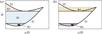
mode group. Five possible resonance mechanisms are depicted schematically in figure 16.
In the first three types of resonances, which are represented in figure 16(a), the upstream/downstream loop is formed entirely by propagative waves. The first type of resonance (denoted R1) can occur at frequencies between the value of the S1 curve at
 $x=0$
and the minimum value of the S2 curve. At these frequencies, a propagative
 $k^{+}$
duct-like wave will encounter an S1 turning point and therefore be reflected as a propagative
 $k^{-}$
duct-like mode. The reflected duct-like mode propagates until is encounters the nozzle plane at
 $x=0$
, at which point it is reflected in accordance with the matrix of reflection coefficients dictated by the the impedance boundary condition. Assuming that the reflection coefficient between the
 $k^{-}$
and
 $k^{+}$
duct-like modes is non-zero, a propagative
 $k^{+}$
duct-like mode will be reflected back toward the turning point, completing the loop required for resonance.
Schematic depiction of the possible types of resonance involving (a) propagative waves only and (b) both propagative and evanescent waves.

A second type of resonance (R2) is possible at frequencies between the maximum and minimum values of the S2 curve. Here, a propagative
 $k^{+}$
duct-like mode encounters an S2 turning point, and is therefore reflected as a propagative
 $k^{-}$
discrete free-stream mode, which propagates to the nozzle where it is again reflected according to the matrix of reflection coefficients. The loop is completed if the reflection coefficient between the discrete free-stream mode and the
 $k^{+}$
duct-like mode is non-zero.
A third type of resonance (R3), which can occur at frequencies between the minimum value of the S1 curve and its value at
 $x=0$
, is similar to R1, but the propagative
 $k^{-}$
duct-like mode encounters a second S1 turning point before it reaches the nozzle. At the turning point, a propagative
 $k^{+}$
duct-like mode is reflected and propagates back to the original downstream turning point, completing the loop.
Two additional possible resonance mechanisms, which are represented in figure 16(b), involve evanescent waves. The first is similar to R3. The propagative
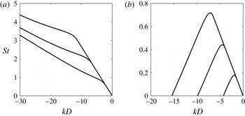
 $k^{-}$
duct-like mode is reflected at the S1 turning point, as in R3, but is also transmitted as an evanescent
 $k^{-}$
duct-like mode. The transmitted wave can be reflected at the nozzle plane as an evanescent
 $k^{+}$
duct-like mode that travels downstream until it again encounters the S1 turning point. It is then reflected as an evanescent
 $k^{-}$
duct-like wave and transmitted as a propagative
 $k^{+}$
duct-like wave. The transmitted wave propagates to the second S1 turning point, where it is reflected as a propagative
 $k^{-}$
duct-like wave, completing the loop.
The final type of resonance (R5) occurs at frequencies between the minimum value of the S2 curve and its value at the merger point of the two saddle points. To understand this scenario, begin with a propagative
 $k^{+}$
duct-like mode at a streamwise position between the S1 and S2 curves. This wave encounters an S1 turning point and is reflected as a propagative
 $k^{-}$
duct-like mode. The reflected wave propagates to the S2 curve but is unaffected because the saddle points on this curve do not involve
 $k^{-}$
duct-like modes (they are formed between a
 $k^{+}$
duct-like mode and a
 $k^{-}$
discrete free-stream mode). The reflected wave therefore propagates all the way to the nozzle plane, where part of the wave is likely reflected as a propagative
 $k^{+}$
duct-like mode. Before this wave can propagate back to its starting point, it is intercepted by an S2 turning point, where it is reflected as a propagative
 $k^{-}$
discrete free-stream mode (as in R2), but also transmitted as an evanescent
 $k^{+}$
duct-like mode. This represents a break in the loop between the
 $k^{-}$
and
 $k^{+}$
propagative waves, but if the transmitted wave does not decay significantly before it reaches the second S2 turning point, where it again becomes propagative, the feedback loop is completed.
Decay rate
 $k_{i}D$
of the
 $k^{+}$
duct-like mode for: (a)
 $m=0$
,
 $n=1$
; (b)
 $m=0$
,
 $n=2$
; (c)
 $m=0$
,
 $n=3$
; (d)
 $m=1$
,
 $n=1$
; (e)
 $m=1$
,
 $n=2$
; (f)
 $m=1$
,
 $n=3$
. The contour levels are distributed on a linear scale and range from
 $\ln (1)=0$
(black) to
 $\ln (0.01)\approx -4.6$
(white).

Whether the R4 and R5 resonance mechanisms are feasible depends on the decay rate of the evanescent waves. Both involve evanescent
 $k^{+}$
duct-like modes, so we address this question by examining the decay rates of these waves. Figure 17 shows contours of
 $k_{i}$
as a function of frequency and streamwise location for the first three radial mode groups at
 $m=0$
and 1. The contour levels are distributed on a linear scale and range from
 $\ln (1)=0$
(black) to
 $\ln (0.01)\approx -4.6$
(white). Waves with
 $k_{i}=\ln (0.01)$
decay by a factor of 100 over a distance of one jet diameter. The S1 and S2 curves are also shown for reference. There are a few noteworthy trends. First, the decay rate is zero in the region bound by the S1, S2 and
 $x=0$
curves, as we already knew. Second, for each mode group, the decay rate is smaller for waves transmitted through S2 turning points than for waves transmitted through S1 turning points. Third, the decay rate for the S2 transmitted waves grow with
 $n$
and are quite small for
 $n=1$
. This suggests that the R5 resonance mechanism is likely to be active for
 $n=1$
, which will be confirmed shortly. This process of transmitting energy through a region that does not support propagative waves (i.e. the region between the two S2 turning points) is analogous to the quantum mechanical concept of tunnelling (Bender & Orszag Reference Bender and Orszag1999; Hall Reference Hall2013).
The wave reflection processes so far described leads to a true resonance only if the
 $k^{+}$
and
 $k^{-}$
waves mutually reinforce one another by interfering constructively rather than destructively. The solutions where constructive reinforcement occurs constitute a set of discrete resonance frequencies. Given the large number of possible resonances and the complicated algebra associated with matching the ‘outer’ WKB solutions on either side of the turning point with the proper ‘inner’ solution, we do not pursue numerical solutions of the problem here. Instead, we address the selection of discrete resonance frequencies in a parallel investigation using global modes of the linearized equations (Schmidt et al.
Reference Schmidt, Towne, Colonius, Cavalieri, Jordan and Brès2017), which confirm that the core modes do resonate at certain discrete frequencies.
4.4 Comparison of weakly non-parallel theory with data
Next, we return to the LES data to assess whether the weakly non-parallel theory describes the global behaviour of the waves within the potential core. Whereas our theoretical model is meant to describe the core waves only, the data are made up of convective disturbances in addition to the acoustic core waves (see, for example, figure 5). To foster a fair comparison, we use the wavenumber decomposition discussed in § 2.5 as a filter to isolate the core waves. The key insight is that the core waves have negative phase velocities while the dominant convective instabilities have positive phase velocities. Therefore, zeroing the positive wavenumber components and taking an inverse streamwise Fourier transform filters out all waves with positive phase velocity, effectively distilling the negative-phase-velocity core waves. This procedure is applied at every radial position to give spatially resolved fields that are dominated by the core waves. Note that the filtering procedure was unnecessary for the local comparisons at the jet inlet in § 3 because the convective disturbances are small there compared to the core waves.
Power spectral density of the phase-velocity-filtered pressure. In the left column (a,c,e,g,i,k)
 $m=0$
and (from top to bottom)
 $St=0.25,0.38,0.39,0.40,0.42,$
and 0.60. In the right column (b,d,f,h,j,l)
 $m=1$
and (from top to bottom)
 $St=0.50,0.62,0.64,0.66,0.69,$
and 0.90. The contour levels are distributed on a logarithmic scale spanning four orders of magnitude. Dashed lines:
 $u_{x}=0.99U_{j}$
. Solid lines show the WKB turning points intrinsic to different resonance mechanisms: (——, blue) R1; (——, green) R2; (——, pink) R5.

The power spectral density of the
 $m=0$
and 1 components of the the phase-velocity-filtered pressure field is plotted in figure 18 for several frequencies. The contour levels are distributed on a logarithmic scale spanning four orders of magnitude, with the maximum level set to the maximum value (over all frequencies) of the power spectral density for the given azimuthal wavenumber. The left (figure 18
a–c) and right (figure 18
d–f) columns contain six frequencies at
 $m=0$
and
 $m=1$
, respectively (the frequencies are different for the two azimuthal wavenumbers). The dashed line in each subplot shows the
 $\bar{u}_{x}=0.99U_{j}$
contour, which serves as a proxy for the outer boundary of the potential core. When present, the solid vertical lines give the streamwise locations of a WKB turning point at the corresponding frequency.
Figure 18(a,b) corresponds to frequencies (
 $St=0.25$
and 0.50 for
 $m=0$
and 1, respectively) that are below the cut-on frequency of the
 $n=1$
duct-like modes. The energy levels at these frequencies are about three orders of magnitude below the maximum, and exhibit no particular concentration in the potential-core region. This is consistent with the model: since no propagative (or lightly damped)
 $k^{+}$
modes exist at these frequencies, there is no possibility of an accumulation of energy due to resonating core modes.
Figure 18(c–h) correspond to frequencies associated with the R1 resonance mechanism for the
 $n=1$
mode group (
 $St=0.38$
,
 $0.39$
, and
 $0.40$
for
 $m=0$
and
 $St=0.62$
,
 $0.64$
and
 $0.66$
for
 $m=1$
). Accordingly, we expect a region of high energy within the potential core, stretching from the nozzle to the S1 turning point and somewhat beyond due to the finite damping rate of the transmitted evanescent waves. This is precisely what is observed in the data. One especially noteworthy feature of the data is the appearance of distinguishable streamwise nodes and anti-nodes within the resonance region. For example, the three frequencies at
 $m=1$
contain three, five and seven anti-nodes, respectively. This pattern is a result of beating between the
 $k^{+}$
and
 $k^{-}$
waves, which have similar but unequal (slowly varying) wavelengths. As shown in Schmidt et al. (Reference Schmidt, Towne, Colonius, Cavalieri, Jordan and Brès2017), this beating is accurately reproduced by discrete global modes of the jet. This constitutes strong evidence that the observed concentration of energy in the potential core is the result of resonance, rather than some other mechanism. Note that the frequency resolution of the transformed data is too low to unambiguously distinguish the narrow frequency range of the R3 and R4 resonance mechanisms.
Figure 18(i,j) corresponds to frequencies (
 $St=0.42$
and 0.69 for
 $m=0$
and 1, respectively) associated with both the R2 and R5 resonance mechanisms. The two vertical lines in these subplots give the streamwise location of the turning points intrinsic to the two different mechanisms. The turning point closer to the nozzle is the downstream end condition for R2, while the second turning point is the downstream end condition for R5. It appears that the latter mechanism dominates. Recall that the R5 resonance involves tunnelling of evanescent waves that is viable for the
 $(0,1)$
mode group because of the low decay rate of the
 $k^{+}$
duct-like modes at these frequencies. It is not immediately clear why there is little evidence for an R2 resonance. One explanation is that the reflection coefficients for the R2 resonance may be small compared to those for R5. The global modes computed by Schmidt et al. (Reference Schmidt, Towne, Colonius, Cavalieri, Jordan and Brès2017) support this hypothesis; at the relevant frequencies, the S1 turning points associated with the R5 mechanism have a significant impact on the form of the global modes, while the S2 turning points associated with R2 have a lesser impact.
Figure 18(k,l) corresponds to frequencies (
 $St=0.60$
and 0.90 for
 $m=0$
and 1, respectively) well above the cut-off frequency of the
 $n=1$
 $k^{+}$
duct-like mode (and below the cut-on frequency for
 $n=2$
). Accordingly, no resonance is expected. The data show this model prediction to be correct. The high energy concentration in the potential core observed at the previous resonant frequencies has vanished, and the remaining waves are less energetic by almost three orders of magnitude.
Power spectral density of the phase-velocity-filtered pressure: (a)
 $m=0$
,
 $r/D=0$
; (b)
 $m=1$
,
 $r/D=0.1$
. The contours levels are distributed on a logarithmic scale spanning four orders of magnitude. The lines show the locations of the WKB turning points.

Other frequencies can be examined by plotting the power spectral density of the phase-velocity-filtered pressure data at a fixed radial position as a function of frequency and streamwise position. Figure 19 shows these data at
 $r/D=0$
and 0.1 for
 $m=0$
and 1, respectively. The contours levels are again distributed on a logarithmic scale spanning four orders of magnitude. This visualization of the data makes it clear that the core waves are energetic primarily within regions of
 $x-St$
space that support a resonance of propagative waves, i.e. on the interior of the region bound by the S1, S2 and
 $x=0$
curves. For both azimuthal wavenumbers, there is also significant energy somewhat farther downstream and at slightly higher frequencies for the first radial mode group. This is explained by the lower damping rate for
 $n=1$
waves transmitted through S2 turning points, as shown in figure 17, and suggests the existence of a sixth resonance entirely composed of lightly damped waves.
5 Model predictions for other operating conditions
The near-nozzle tones that are generated by the acoustic resonance in the potential core have been experimentally observed for only certain combinations of Mach number and temperature ratio. In this section, we will use the vortex-sheet model to explain this observation and to provide a rough guideline for when the resonance and resulting tones will and will not be present. At first glance, the vortex-sheet model may appear ill suited for this task since it is a strictly parallel representation of the jet and therefore cannot predict the turning points necessary for resonance and the formation of tones. However, in the isothermal Mach 0.9 jet, the two vortex-sheet saddle points approximately bound the frequencies for which there exist both
 $k^{+}$
and
 $k^{-}$
propagative waves, which is a necessary ingredient for resonance, and provide a good approximation of the tonal frequencies (see figure 10). As we consider jets with other Mach numbers and temperature ratios, we will use the existence of a limited range of frequencies for which both
 $k^{+}$
and
 $k^{-}$
propagative waves exist for the same core-mode group as a criterion to decide whether or not tones are likely to be observed.
5.1 Mach number dependence
We first investigate the Mach number dependence of the core modes at a fixed temperature ratio. Specifically, the
 $(k,\unicode[STIX]{x1D714})$
coordinates of the vortex-sheet and duct saddle points are calculated as a function of the Mach number at
 $T=1$
. The results for
 $(m=0,n=0)$
are shown in figure 20.
Saddle-point locations as a function of Mach number for the vortex sheet (——) and the duct (– – –). Bifurcations exist at
 $M=0.82$
and
 $M=1$
.

At
 $M=0.9$
, the vortex-sheet modes form two saddle points as shown in figure 8. Moving toward smaller Mach numbers, a bifurcation is encountered at
 $M=0.82$
at which the two saddle points merge and move off the real
 $k$
and
 $\unicode[STIX]{x1D714}$
axes. To exemplify the situation beyond the bifurcation point, the saddle points for
 $M=0.6$
are shown in figure 21(a). The saddle point with
 $\unicode[STIX]{x1D714}_{i}>0$
occurs between two
 $k^{-}$
modes and is therefore irrelevant. The saddle with
 $\unicode[STIX]{x1D714}_{i}<0$
occurs between a
 $k^{+}$
mode and
 $k^{-}$
mode, and is therefore valid. Accordingly, the core modes are absolutely stable for
 $M<0.82$
. This bifurcation is not predicted by the duct model; the duct modes remain neutrally stable for all subsonic Mach numbers.
Moving now from
 $M=0.9$
toward higher Mach numbers, we encounter a different kind of bifurcation at
 $M=1$
. The S2 vortex-sheet saddle point continues on the real axes unaffected by the switch from subsonic to supersonic flow, but the S1 saddle point asymptotically approaches zero frequency and a negative infinite wavenumber, never crossing
 $M=1$
. This behaviour is accurately predicted by the duct saddle point as given by (3.20) and (3.21). Therefore, for
 $M>1$
, there is one saddle point on the real axes. The saddle point for
 $M=1.5$
is shown in figure 21(b).
Saddle points for the
 $(0,1)$
mode group of the vortex sheet for
 $T=1$
and (a)
 $M=0.6$
(b)
 $M=1.5$
. Lines of varying
 $\unicode[STIX]{x1D714}_{r}$
and: (——)
 $\unicode[STIX]{x1D714}_{i}=0$
; (– – –)
 $\unicode[STIX]{x1D714}_{i}<0$
; (– ⋅ – ⋅ –)
 $\unicode[STIX]{x1D714}_{i}>0$
.

The number of neutral saddle points on the real
 $k$
-axis – zero for
 $M<0.82$
, two for
 $0.82<M<1$
, and one for
 $M>1$
– has a profound impact on the types of core waves supported by the jet. The dispersion relation of the
 $(0,1)$
propagative waves for
 $M=0.9$
, which lies in the intermediate region, was shown in figure 9. Since there is a distinct frequency range, bounded by the two saddle points, for which both
 $k^{+}$
and
 $k^{-}$
waves exist, the previously described resonance is possible at certain frequencies but not others, leading to spectral tones. Figure 22 shows the dispersion relation of the
 $(0,1)$
propagative waves for
 $M=0.6$
and
 $M=1.5$
, which serve as examples for the low and high Mach number ranges. For
 $M=0.6$
, there exist only
 $k^{-}$
propagative waves at all frequencies since there are no saddle points on the real axes, and therefore no upstream/downstream transition. Since only
 $k^{-}$
waves are supported by the flow, no resonance is possible, precluding the possibility of tones. For
 $M=1.5$
, there exist both
 $k^{+}$
and
 $k^{-}$
waves at the same frequencies due to the presence of a single saddle point on the real axis. Accordingly, there is the possibility of resonance, but this resonance mechanism exists at all frequencies, resulting in broadband energy distribution rather than discrete tones.
Dispersion relations of the propagative waves for the first three
 $m=0$
radial mode groups of the vortex sheet at
 $T=1$
and (a)
 $M=0.6$
and (b)
 $M=1.5$
. The analogous dispersion relations for
 $M=0.9$
appear in figure 9.

Our results at
 $M=0.6$
and
 $M=1.5$
are consistent with the findings of Tam & Hu (Reference Tam and Hu1989). They referred to the core modes described in this paper as ‘subsonic instability modes’, and noted that only
 $k^{-}$
waves exist for
 $M=0.6$
while both
 $k^{-}$
and
 $k^{+}$
propagative waves exist for
 $M=1.5$
and other supersonic Mach numbers. However, they did not investigate the transition between these two cases that gives rise to the interesting resonances discussed in this paper.
To summarize, the vortex-sheet model suggests that only jets within a limited Mach number range,
 $0.82<M<1$
for
 $T=1$
, have two saddle points on the real axes, which is a key ingredient for generating tones. However, it is appropriate at this stage to reflect on the fact that we are analysing a turbulent flow based on a linearization about the mean. Perturbations to the mean flow field could broaden the range of resonating Mach numbers, and lightly damped modes that are excited by turbulence could also participate in the resonance (as we already observed in § 4.3). Therefore, we speculate that the tones should gradually appear as the Mach number approaches 0.82 and reach their strongest resonance before dissolving away again into a broadband spectrum for
 $M>1$
.
5.2 Temperature ratio dependence
Finally, the temperature ratio dependence of the core modes is incorporated into the analysis with the goal of determining certain Mach number, temperature ratio combinations that support two neutral saddle points. Specifically, the two Mach number bifurcation points described in the previous subsection for
 $T=1$
that bound the two-saddle-point region are computed as a function of temperature ratio.
The results are summarized for
 $m=0$
and 1 in figure 23. The solid curve represents the supersonic bifurcation, which occurs when
 $M_{j}=1$
irrespective of the temperature ratio for all mode groups. This behaviour is exactly predicted by the duct model based on (3.20); the duct saddle point asymptotically vanishes when
 $M_{j}\rightarrow 1$
(i.e.
 $M^{2}\rightarrow T$
) for all
 $\unicode[STIX]{x1D6FD}_{m,n}$
. On the other hand, the subsonic bifurcation point is not predicted by the duct model and its location is a weak function of
 $n$
. The three dashed curves, from top to bottom, show the bifurcation point for
 $n=0$
, 1 and 2, respectively. The spacing between the curves decreases with increasing
 $n$
, suggesting the existence of an asymptotic curve that bounds the region for all
 $n$
.
Saddle-point bifurcations as a function of Mach number and temperature ratio for (a)
 $m=0$
and (b)
 $m=1$
. Black curve: supersonic bifurcation. Other curves: subsonic bifurcation. Shaded region: operating conditions where the model predicts the existence of tones. Closed symbols: jets in which tones have been observed. Open symbols: jets in which tones have not been observed. Squares: computational jets. Circles: experimental jets.

The shaded region demarcates the Mach number, temperature ratio combinations between the two bifurcations (up to
 $n=3$
). For these values, two saddle points exist and tones are therefore expected to be present in the near-nozzle region outside of the jet. The lower boundary should not be viewed as a precise limit, however, since tones likely exist at somewhat lower Mach numbers, as discussed in the previous section. These predictions can be compared to the aforementioned experimental and numerical observations of near-nozzle tones. The filled and open symbols represent jet set points where tones have and have not been observed, respectively. The circles correspond to results from Suzuki & Colonius (Reference Suzuki and Colonius2006) while the squares correspond to two LES databases, including the Mach 0.9 isothermal jet used throughout the paper. The agreement between the model predictions and the experimental and numerical observations is excellent, especially if we permit ourselves to blur the lower boundary of resonance in accordance with comments at the end of § 5.1.
6 Summary and discussion
We have used LES data from a Mach 0.9 isothermal, turbulent jet along with parallel and weakly non-parallel linear modal analysis to investigate trapped waves that are observed within the potential core of the jet and detected as tones outside of the jet in the near-nozzle region. Three types of waves are identified. The first two approximately satisfy the dispersion relation for a soft duct and can therefore be understood as
 $k^{+}$
and
 $k^{-}$
duct-like acoustic modes. These waves experience the shear-layer as a pressure-release surface and are therefore radially confined to the potential core. The third type of wave is a
 $k^{-}$
mode and represents a weak coupling between the jet core and the free stream. Each of these modes are either cut-on or cut-off depending on frequency and (for the weakly non-parallel model) streamwise location, and the cut-on/cut-off transition points correspond to saddle points in the complex wavenumber plane. Within the weakly non-parallel model, these saddle points also constitute turning points of the asymptotic WKB approximation that provide a mechanism by which
 $k^{+}$
waves can be converted into
 $k^{-}$
waves, and vice versa. Paired with a second end condition provided by the nozzle, this leads to the possibility of resonance within the limited frequency bands that contain turning points. The resonance mechanisms are further investigated and refined by the parallel global analysis of Schmidt et al. (Reference Schmidt, Towne, Colonius, Cavalieri, Jordan and Brès2017).
Drawing on these results, a vortex-sheet model is used to explore the effect of Mach number and temperature ratio on the trapped waves. It is found that, for isothermal jets, the necessary conditions for resonance between propagative waves exist only for
 $0.82<M<1$
, but that the possibility of lightly damped resonance persists at somewhat lower Mach numbers. The upper limit is the same for all temperature ratios, indicating that the jet must be subsonic, while the lower limit is a function of temperature ratio.
Our three simple models capture with surprising accuracy numerous aspects of the trapped waves that are extracted from the LES data. The model dispersion relations closely follow the empirical dispersion relations obtained through frequency–wavenumber decomposition of the data. The frequency bands between the two saddle points predict the tonal frequencies. The radial structure of the pressure field near the nozzle is accurately described by the eigenfunctions of the core modes. The turning point analysis and the resulting resonance mechanisms provide predictions for the frequency and spatial energy distribution of the trapped waves that closely match the data. These results confirm that the models capture the essential physics of the potential core waves. Similar comparisons with simulation or experimental data will be required to further analyse the predictions obtained from the vortex-sheet model at other Mach numbers and temperature ratios.
Whether or not these trapped waves are important to the overall jet dynamics or acoustics remains to be established. An ongoing experimental campaign (Jaunet et al. Reference Jaunet, Jordan, Cavalieri, Towne, Colonius, Schmidt and Brès2016) suggests that the trapped waves can be observed in the far-field acoustic spectrum at angles nearly tangent to the jet, and that these tones appear to be related to the R2 resonance mechanism. The latter result is consistent with the slower radial decay of the discrete free-stream modes that participate in this resonance mechanism. The same experimental investigation also suggests that the trapped waves are responsible for strong tones that are observed in the acoustic field when a solid edge is introduced near the jet. Previous attempts to explain these edge tones assumed a Rossiter-like scenario (Lawrence & Self Reference Lawrence and Self2015; Zaman et al. Reference Zaman, Fagan, Bridges and Brown2015) and have not yielded an accurate model. The analysis presented in this paper could provide the necessary building blocks to explain and model these edge tones.
Acknowledgements
A.T. and T.C. gratefully acknowledge support from the Office of Naval Research under contract N0014-11-1-0753. A.V.G.C. and P.J. acknowledge support from the Science Without Borders project no. A073/2013. OTS was supported by DFG grant no. 3114/1-1. The LES study was supported by NAVAIR SBIR project, under the supervision of Dr J. T. Spyropoulos. The main LES calculations were carried out on CRAY XE6 machines at DoD HPC facilities in ERDC DSRC. The authors also thank S. Piantanida and R. Kari for performing the experimental measurements reported in figures 3 and 10.
Appendix A. Linearized Euler equations
We write the compressible Euler equations in cylindrical coordinates in terms of specific volume
 $\unicode[STIX]{x1D708}$
, streamwise velocity
 $u_{x}$
, radial velocity
 $u_{r}$
, azimuthal velocity
 $u_{\unicode[STIX]{x1D703}}$
and pressure
 $p$
:
 $$\begin{eqnarray}\displaystyle & \displaystyle \frac{\text{D}\unicode[STIX]{x1D708}}{\text{D}t}-\unicode[STIX]{x1D708}(\unicode[STIX]{x1D735}\boldsymbol{\cdot }u)=0, & \displaystyle\end{eqnarray}$$
 $$\begin{eqnarray}\displaystyle & \displaystyle \frac{\text{D}u_{x}}{\text{D}t}+\unicode[STIX]{x1D708}\frac{\unicode[STIX]{x2202}p}{\unicode[STIX]{x2202}x}=0, & \displaystyle\end{eqnarray}$$
 $$\begin{eqnarray}\displaystyle & \displaystyle \frac{\text{D}u_{r}}{\text{D}t}-\frac{u_{\unicode[STIX]{x1D703}}^{2}}{r}+\unicode[STIX]{x1D708}\frac{\unicode[STIX]{x2202}p}{\unicode[STIX]{x2202}r}=0, & \displaystyle\end{eqnarray}$$
 $$\begin{eqnarray}\displaystyle & \displaystyle \frac{\text{D}u_{\unicode[STIX]{x1D703}}}{\text{D}t}+\frac{u_{r}u_{\unicode[STIX]{x1D703}}}{r}+\frac{\unicode[STIX]{x1D708}}{r}\frac{\unicode[STIX]{x2202}p}{\unicode[STIX]{x2202}\unicode[STIX]{x1D703}}=0, & \displaystyle\end{eqnarray}$$
 $$\begin{eqnarray}\displaystyle & \displaystyle \frac{\text{D}p}{\text{D}t}+\unicode[STIX]{x1D6FE}p(\unicode[STIX]{x1D735}\boldsymbol{\cdot }u)=0, & \displaystyle\end{eqnarray}$$
 $$\begin{eqnarray}\frac{\text{D}}{\text{D}t}=\frac{\unicode[STIX]{x2202}}{\unicode[STIX]{x2202}t}+u_{x}\frac{\unicode[STIX]{x2202}}{\unicode[STIX]{x2202}x}+u_{r}\frac{\unicode[STIX]{x2202}}{\unicode[STIX]{x2202}r}+\frac{u_{\unicode[STIX]{x1D703}}}{r}\frac{\unicode[STIX]{x2202}}{\unicode[STIX]{x2202}\unicode[STIX]{x1D703}}\end{eqnarray}$$
and
 $$\begin{eqnarray}\unicode[STIX]{x1D735}\boldsymbol{\cdot }u=\frac{\unicode[STIX]{x2202}u_{x}}{\unicode[STIX]{x2202}x}+\frac{\unicode[STIX]{x2202}u_{r}}{\unicode[STIX]{x2202}r}+\frac{u_{r}}{r}+\frac{1}{r}\frac{\unicode[STIX]{x2202}u_{\unicode[STIX]{x1D703}}}{\unicode[STIX]{x2202}\unicode[STIX]{x1D703}}.\end{eqnarray}$$
All variables have been appropriately non-dimensionalized by the ambient sound speed
 $c_{\infty }$
and density
 $\unicode[STIX]{x1D70C}_{\infty }$
and the nozzle diameter
 $D$
. The fluid is approximated as a perfect gas with specific heat ratio
 $\unicode[STIX]{x1D6FE}$
. For the state vector
 $\boldsymbol{q}=\{\unicode[STIX]{x1D708},u_{x},u_{y},u_{\unicode[STIX]{x1D703}},p\}^{\text{T}}$
, the linearized Euler operators defined in (3.11) are:
 $$\begin{eqnarray}\unicode[STIX]{x1D63C}_{x}=\left[\begin{array}{@{}ccccc@{}}\displaystyle \bar{u}_{x} & -\bar{\unicode[STIX]{x1D708}} & 0 & 0 & 0\\ \displaystyle 0 & \bar{u}_{x} & 0 & 0 & \bar{\unicode[STIX]{x1D708}}\\ \displaystyle 0 & 0 & \bar{u}_{x} & 0 & 0\\ \displaystyle 0 & 0 & 0 & \bar{u}_{x} & 0\\ \displaystyle 0 & \unicode[STIX]{x1D6FE}\bar{p} & 0 & 0 & \bar{u}_{x}\end{array}\right],\quad \unicode[STIX]{x1D63C}_{r}=\left[\begin{array}{@{}ccccc@{}}\displaystyle \bar{u}_{r} & 0 & -\bar{\unicode[STIX]{x1D708}} & 0 & 0\\ \displaystyle 0 & \bar{u}_{r} & 0 & 0 & 0\\ \displaystyle 0 & 0 & \bar{u}_{r} & 0 & \bar{\unicode[STIX]{x1D708}}\\ \displaystyle 0 & 0 & 0 & \bar{u}_{r} & 0\\ \displaystyle 0 & 0 & \unicode[STIX]{x1D6FE}\bar{p} & 0 & \bar{u}_{r}\end{array}\right],\end{eqnarray}$$
 $$\begin{eqnarray}\unicode[STIX]{x1D63C}_{\unicode[STIX]{x1D703}}=\frac{1}{r}\left[\begin{array}{@{}ccccc@{}}\displaystyle \bar{u}_{\unicode[STIX]{x1D703}} & 0 & 0 & -\bar{\unicode[STIX]{x1D708}} & 0\\ \displaystyle 0 & \bar{u}_{\unicode[STIX]{x1D703}} & 0 & 0 & 0\\ \displaystyle 0 & 0 & \bar{u}_{\unicode[STIX]{x1D703}} & 0 & 0\\ \displaystyle 0 & 0 & 0 & \bar{u}_{\unicode[STIX]{x1D703}} & \bar{\unicode[STIX]{x1D708}}\\ \displaystyle 0 & 0 & 0 & \unicode[STIX]{x1D6FE}\bar{p} & \bar{u}_{\unicode[STIX]{x1D703}}\end{array}\right],\quad \unicode[STIX]{x1D63C}_{0}=\left[\begin{array}{@{}ccccc@{}}\displaystyle -\bar{\unicode[STIX]{x1D6F7}} & \displaystyle \frac{\unicode[STIX]{x2202}\bar{\unicode[STIX]{x1D708}}}{\unicode[STIX]{x2202}x} & \displaystyle \frac{\unicode[STIX]{x2202}\bar{\unicode[STIX]{x1D708}}}{\unicode[STIX]{x2202}r}-\frac{\bar{\unicode[STIX]{x1D708}}}{r} & 0 & 0\\ \displaystyle \frac{\unicode[STIX]{x2202}\bar{p}}{\unicode[STIX]{x2202}x} & \displaystyle \frac{\unicode[STIX]{x2202}\bar{u}_{x}}{\unicode[STIX]{x2202}x} & \displaystyle \frac{\unicode[STIX]{x2202}\bar{u}_{x}}{\unicode[STIX]{x2202}r} & 0 & 0\\ \displaystyle \frac{\unicode[STIX]{x2202}\bar{p}}{\unicode[STIX]{x2202}r} & \displaystyle \frac{\unicode[STIX]{x2202}\bar{u}_{r}}{\unicode[STIX]{x2202}x} & \displaystyle \frac{\unicode[STIX]{x2202}\bar{u}_{r}}{\unicode[STIX]{x2202}r} & 0 & 0\\ \displaystyle 0 & \displaystyle \frac{\unicode[STIX]{x2202}\bar{u}_{\unicode[STIX]{x1D703}}}{\unicode[STIX]{x2202}x} & \displaystyle \frac{\unicode[STIX]{x2202}\bar{u}_{\unicode[STIX]{x1D703}}}{\unicode[STIX]{x2202}r}+\frac{\bar{u}_{\unicode[STIX]{x1D703}}}{r} & \displaystyle \frac{1}{r}\bar{u}_{r} & 0\\ \displaystyle 0 & \displaystyle \frac{\unicode[STIX]{x2202}\bar{p}}{\unicode[STIX]{x2202}x} & \displaystyle \frac{\unicode[STIX]{x2202}\bar{p}}{\unicode[STIX]{x2202}r}+\frac{\unicode[STIX]{x1D6FE}\bar{p}}{r} & 0 & \unicode[STIX]{x1D6FE}\bar{\unicode[STIX]{x1D6F7}}\end{array}\right],\end{eqnarray}$$
where
 $\bar{\unicode[STIX]{x1D6F7}}=\unicode[STIX]{x1D735}\boldsymbol{\cdot }\bar{\boldsymbol{u}}$
.
Appendix B. Derivation of the vortex-sheet dispersion relation
The cylindrical vortex sheet is governed by the compressible Euler equations linearized about inner and outer regions of uniform flow. These equations can be reduced to a Helmholtz equation for the pressure in each region:
 $$\begin{eqnarray}\displaystyle & \displaystyle \left[\left(\frac{\unicode[STIX]{x2202}}{\unicode[STIX]{x2202}t}+M\frac{\unicode[STIX]{x2202}}{\unicode[STIX]{x2202}x}\right)^{2}-T\unicode[STIX]{x1D6FB}^{2}\right]p_{i}=0, & \displaystyle\end{eqnarray}$$
 $$\begin{eqnarray}\displaystyle & \displaystyle \left[\frac{\unicode[STIX]{x2202}}{\unicode[STIX]{x2202}t}^{2}-\unicode[STIX]{x1D6FB}^{2}\right]p_{o}=0. & \displaystyle\end{eqnarray}$$
 $$\begin{eqnarray}\left[\frac{\unicode[STIX]{x2202}^{2}}{\unicode[STIX]{x2202}r^{2}}+\frac{1}{r}\frac{\unicode[STIX]{x2202}}{\unicode[STIX]{x2202}r}-\unicode[STIX]{x1D6FE}_{i,o}^{2}-\frac{m^{2}}{r^{2}}\right]\hat{p}_{i,o}(r)=0,\end{eqnarray}$$
with
 $\unicode[STIX]{x1D6FE}_{i}$
and
 $\unicode[STIX]{x1D6FE}_{o}$
given by (3.16). As stated previously, all quantities have been normalized by the jet diameter and outer thermodynamic quantities such that
 $M=U_{j}/c_{\infty }$
is the acoustic Mach number and
 $T=T_{j}/T_{\infty }$
is the temperature ratio.
Enforcing boundedness at the centreline and at infinity leads to the solutions
 $$\begin{eqnarray}p_{i}(r)=C_{i}\text{I}_{m}(\unicode[STIX]{x1D6FE}_{i}r)\end{eqnarray}$$
at the inner part of the sheet, and
 $$\begin{eqnarray}p_{o}(r)=C_{o}\text{K}_{m}(\unicode[STIX]{x1D6FE}_{o}r)\end{eqnarray}$$
in the outer flow. These two functions should be matched at the vortex-sheet location
 $r=1/2$
, which leads to
 $$\begin{eqnarray}\displaystyle & \displaystyle p_{i}({\textstyle \frac{1}{2}})=p_{o}({\textstyle \frac{1}{2}}), & \displaystyle\end{eqnarray}$$
 $$\begin{eqnarray}\displaystyle & \displaystyle \frac{\text{d}p_{i}}{\text{d}r}\left(\frac{1}{2}\right)=\frac{(\unicode[STIX]{x1D714}-kM)^{2}}{T\unicode[STIX]{x1D714}^{2}}\frac{\text{d}p_{o}}{\text{d}r}\left(\frac{1}{2}\right), & \displaystyle\end{eqnarray}$$
 $\unicode[STIX]{x1D702}$
from
 $$\begin{eqnarray}\displaystyle & \displaystyle (\unicode[STIX]{x1D714}-kM)^{2}\unicode[STIX]{x1D702}=T\frac{\text{d}p_{i}}{\text{d}r}\left(\frac{1}{2}\right), & \displaystyle\end{eqnarray}$$
 $$\begin{eqnarray}\displaystyle & \displaystyle \unicode[STIX]{x1D714}^{2}\unicode[STIX]{x1D702}=\frac{\text{d}p_{o}}{\text{d}r}\left(\frac{1}{2}\right). & \displaystyle\end{eqnarray}$$
 $C_{i}$
and
 $C_{o}$
from (B 5a
) and (B 5b
).
Appendix C. Derivation of the soft duct dispersion relation
An inviscid flow inside a duct is governed by the Euler equations linearized about a uniform velocity, which can be reduced to the same Helmholtz equation that governs the inner stream of the vortex-sheet model. All quantities have been normalized by the duct diameter and ambient thermodynamic quantities so that non-dimensional quantities are consistent with those in the linearized Euler and vortex-sheet models. Enforcing boundedness at the centreline leads to the solution
 $$\begin{eqnarray}p_{d}(r)=C_{d}\text{I}_{m}\left(\unicode[STIX]{x1D6FE}_{i}r\right)\end{eqnarray}$$
and enforcing a homogeneous Dirichlet boundary condition at the duct wall,
 $$\begin{eqnarray}\hat{p}_{d}({\textstyle \frac{1}{2}})=0,\end{eqnarray}$$
implies that
 $$\begin{eqnarray}\text{I}_{m}\left(\frac{\unicode[STIX]{x1D6FE}_{i}}{2}\right)=0.\end{eqnarray}$$
Using the relationship between
 $\text{I}_{m}$
and
 $\text{J}_{m}$
, equation (C 3) leads to the soft duct dispersion relation (3.18).