



1 Introduction
An improved understanding of gas–solid heat transfer is crucial for design and scale-up of process equipment in many industries, such as biomass fast pyrolysis (Brown Reference Brown2011), chemical looping combustion (Shen et al.
Reference Shen, Zheng, Xiao and Xiao2008) and
 $\text{CO}_{2}$
capture (Abanades et al.
Reference Abanades, Anthony, Lu, Salvador and Alvarez2004; Yi et al.
Reference Yi, Jo, Seo, Lee and Ryu2007). Instead of conducting expensive experiments, multiphase computational fluid dynamics (CFD) (Syamlal, Rogers & O’Brien Reference Syamlal, Rogers and O’Brien1993; Kashiwa & Gaffney Reference Kashiwa and Gaffney2003; Sun, Battaglia & Subramaniam Reference Sun, Battaglia and Subramaniam2007) is increasingly being used for reactor scale-up from laboratory to pilot and full-scale plants, and also for evaluation of different design options (Halvorsen, Guenther & O’Brien Reference Halvorsen, Guenther and O’Brien2003). Device-scale multiphase CFD simulations are usually based on the Eulerian–Eulerian two-fluid model (Anderson & Jackson Reference Anderson and Jackson1967; Drew & Passman Reference Drew and Passman1998) in which averaged equations for conservation of mass, momentum and energy are given for each phase, with coupling terms representing the interphase interactions. These equations contain unclosed terms that need to be modelled accurately, since the predictive capability of multiphase CFD simulations depends on the accuracy of models for interphase exchange of species, momentum and heat.
In the absence of mass transfer between phases, the average fluid temperature equation from two-fluid theory (Syamlal et al. Reference Syamlal, Rogers and O’Brien1993; Garg Reference Garg2009) reads as follows:
 $$\begin{eqnarray}\displaystyle & & \displaystyle \underbrace{\frac{\partial }{\partial t}\{{\it\rho}_{f}{\it\varepsilon}_{f}c_{pf}\langle T^{(f)}\rangle \}}_{\text{unsteady term}}+\underbrace{{\displaystyle \frac{\partial }{\partial x_{j}}}\{{\it\rho}_{f}{\it\varepsilon}_{f}c_{pf}\langle u_{j}^{(f)}\rangle \langle T^{(f)}\rangle \}}_{\text{mean flow convection}}\nonumber\\ \displaystyle & & \displaystyle \quad =\underbrace{\left\langle {\displaystyle \frac{\partial I_{f}}{\partial x_{j}}}q_{j}\right\rangle }_{\substack{ \text{(1) average gas{-}solid} \\ \text{heat transfer}}}-\underbrace{{\displaystyle \frac{\partial }{\partial x_{j}}}\langle I_{f}q_{j}\rangle }_{\substack{ \text{(2) average conduction} \\ \text{in the fluid phase}}}-\underbrace{\frac{\partial }{\partial x_{j}}\{{\it\rho}_{f}c_{pf}\langle I_{f}u_{j}^{\prime \prime (f)}T^{\prime \prime (f)}\rangle \}}_{\substack{ \text{(3) pseudo-turbulent} \\ \text{heat flux term}}},\end{eqnarray}$$
and it contains the following unclosed terms:
-
(1) average gas–solid heat transfer;
-
(2) average conduction in the fluid phase; and
-
(3) transport term involving the pseudo-turbulent heat flux
 ${\it\rho}_{f}c_{pf}\langle I_{f}u_{j}^{\prime \prime (f)}T^{\prime \prime (f)}\rangle$
arising from temperature–velocity covariance.
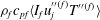
In (1.1),
 ${\it\rho}_{f}$
and
 $c_{pf}$
are the density and specific heat of the fluid phase, respectively,
 $q_{j}=-k_{f}\partial T/\partial x_{j}$
is the heat flux vector and
 ${\it\varepsilon}_{f}=\langle I_{f}\rangle$
is the average volume fraction of the fluid phase, where
 $I_{f}(\boldsymbol{x},t)$
is the fluid-phase indicator function that is unity if the point
 $\boldsymbol{x}$
lies on the fluid phase at time
 $t$
, and zero otherwise. If
 ${\it\psi}(\boldsymbol{x},t)$
is any field (velocity or temperature), then its phasic average
 $\langle {\it\psi}^{(f)}\rangle (\boldsymbol{x},t)$
(e.g. the average fluid velocity
 $\langle u_{j}^{(f)}\rangle$
and average fluid temperature
 $\langle T^{(f)}\rangle$
) is its average value conditional on being in the fluid phase, which is defined as:
 $$\begin{eqnarray}\langle {\it\psi}^{(f)}\rangle (\boldsymbol{x},t)=\frac{\langle I_{f}(\boldsymbol{x},t){\it\psi}(\boldsymbol{x},t)\rangle }{\langle I_{f}(\boldsymbol{x},t)\rangle }.\end{eqnarray}$$
We use angle brackets to denote ensemble averaging of random fields over all particle configurations and an overbar to indicate spatial averages (in this problem these spatial averages appear either as a cross-sectional average of a random field that depends on the particle configuration, or as a streamwise average of an inhomogeneous ensemble-averaged field.) Using the phasic average, the fluctuating components of the fluid velocity and temperature in (1.1) are defined as
 $u_{j}^{\prime \prime (f)}=u_{j}-\langle u_{j}^{(f)}\rangle$
and
 $T^{\prime \prime (f)}=T-\langle T^{(f)}\rangle$
, where these fluctuations depend on spatial location and time, although for brevity this dependence is not explicitly shown. The average fluid velocity is obtained by solving the averaged momentum and mass conservation equations. In order to solve (1.1) for the average fluid temperature, closure models are needed for terms (1)–(3). In a typical two-fluid simulation of gas–solid flow, this equation is coupled to a similar averaged temperature equation for the solid phase (Hrenya & Morris Reference Hrenya and Morris2014), but this work only focuses on models for the unclosed terms in the average fluid temperature equation. In a recent study (Sun, Tenneti & Subramaniam Reference Sun, Tenneti and Subramaniam2015) the average gas–solid heat transfer term was quantified and modelled. This study focuses on quantification and modelling of the pseudo-turbulent heat flux that arises from the temperature–velocity covariance, and average conduction in the fluid phase.
The transport term (3) in the average fluid temperature equation (1.1) arises from correlation of gas-phase velocity and temperature fluctuations that result in a pseudo-turbulent heat flux, and it is typically neglected in CFD simulations. These gas-phase velocity fluctuations can arise from turbulence inherent in the gas phase, or they can be generated by wakes resulting from the interaction of particles with the mean slip velocity between the gas and solid phases. The second mechanism can generate gas-phase velocity fluctuations even in laminar gas–solid flow and these are termed pseudo-turbulent velocity fluctuations. They arise due to spatio-temporal fluctuations in the fluid velocity, and in steady flows their primary contribution is from the spatial variation of fluid velocity due to the presence of particles in a flow with a non-zero mean slip velocity. The kinetic energy associated with these fluctuations is called the pseudo-turbulent kinetic energy (PTKE). Mehrabadi, Tenneti & Subramaniam (Reference Mehrabadi, Tenneti and Subramaniam2015) have quantified PTKE in fixed particle assemblies and freely evolving suspensions, and have shown that the level of PTKE is a significant fraction of the kinetic energy associated with the mean slip velocity. Similarly, the temperature–velocity covariance results in a pseudo-turbulent heat flux (PTHF), which needs to be quantified in non-isothermal gas–solid flow.
The study of pseudo-turbulent heat flux in fixed bed heat transfer is closely related to the mass transfer problem of a solute dispersing in a porous medium or a bed of particles. Together these may be termed the passive scalar transport problem provided the effects of free convection can be neglected. There are several theoretical studies related to hydrodynamic dispersion in a random fixed bed of particles (Koch & Brady Reference Koch and Brady1985, Reference Koch and Brady1987a ,Reference Koch and Brady b ) or a periodic porous medium (Brenner & Gaydos Reference Brenner and Gaydos1977; Brenner Reference Brenner1980; Edwards et al. Reference Edwards, Shapiro, Brenner and Shapira1991) in Stokes or low Reynolds number flow.
Koch & Brady (Reference Koch and Brady1985) solved the convection–diffusion equation for mass transfer in Stokes flow through fixed beds using an asymptotic analysis that is valid in the dilute limit (low solid volume fraction). In their analysis, Koch & Brady (Reference Koch and Brady1985) assumed a linear concentration profile that varies slowly (on the length scale of the one-particle problem) in the axial direction. Koch & Brady (Reference Koch and Brady1985) decompose the mean flux as the sum of a mean convective term and an effective diffusive flux, which includes the covariance of concentration and velocity (the analogue of PTHF). They obtained the dependence of the effective diffusivity
 $D_{eff}$
on the Péclet number (
 $Pe=Ua/D_{f}$
), which characterizes the ratio of convective effects to diffusive effects. Here
 $U$
is the superficial fluid velocity,
 $a$
is the particle diameter and
 $D_{f}$
is the molecular diffusivity of the solute. At low Péclet number (
 $Pe=Ua/D_{f}<1$
) they obtained a
 $Pe^{2}$
dependence, whereas at high Péclet number they obtained terms proportional to
 $Pe$
and
 $Pe\ln (Pe)$
. The linear dependence is attributed to the mechanical dispersion mechanism while the
 $Pe\ln (Pe)$
dependency is attributed to a non-mechanical dispersion mechanism that arises from the no-slip boundary condition (obtained from a boundary layer analysis). Koch’s work provides early evidence that in fixed particle beds the presence of bulk convective motion induces fluid velocity fluctuations (mechanical dispersion) because of the presence of particles, and this is an important factor affecting macrotransport.
Hydrodynamic dispersion as described by Brenner and others treats the dispersion of solute particles through periodic porous media (Brenner Reference Brenner1980; Lowe & Frenkel Reference Lowe and Frenkel1996; Manz, Gladden & Warren Reference Manz, Gladden and Warren1999; Capuani, Frenkel & Lowe Reference Capuani, Frenkel and Lowe2003; Mostaghimi, Bijeljic & Blunt Reference Mostaghimi, Bijeljic and Blunt2012) or randomly placed particles (Maier et al.
Reference Maier, Kroll, Bernard, Howington, Peters and Davis2000, Reference Maier, Kroll, Bernard, Howington, Peters and Davis2003). Brenner (Reference Brenner1980) showed that by considering the evolution equation of the transition probability density
 $P(\boldsymbol{R},t|\boldsymbol{R}^{\prime },t=0)$
for the spatial position of solute molecules, one can formally arrive at the convection–diffusion equation governing the instantaneous concentration
 $c(\boldsymbol{R},t)$
(or solute number density) field, which is nothing but the unnormalized probability density of solute molecule position
 $P(\boldsymbol{R},t)$
. It has been established by several authors (Brenner Reference Brenner1980; Pope Reference Pope1998) that the mean squared displacement of solute molecules, which Brenner showed can be obtained from moments of the transition probability density of the solute particles, is related to the effective diffusivity. The moments of the transition probability density lead to the
 $B$
–field in periodic porous media.
Thermal dispersion in fixed beds or porous media defined by Whitaker (Reference Whitaker1999) and Kaviany (Reference Kaviany2012) based on temperature–velocity covariance and a gradient-diffusion model were studied experimentally (Yagi, Kunii & Wakao Reference Yagi, Kunii and Wakao1960; Özgümüş, Mobedi, Özkol & Nakayama Reference Özgümüş, Mobedi, Özkol and Nakayama2013) and numerically (Kuwahara, Nakayama & Koyama Reference Kuwahara, Nakayama and Koyama1996; Pedras & de Lemos Reference Pedras and de Lemos2008; Jeong & Choi Reference Jeong and Choi2011). In the above experimental and numerical works, local thermal equilibrium between solid and fluid phases is assumed to be valid and the solid surface temperature evolves identically to the fluid temperature in time. Several numerical studies (Kuwahara et al.
Reference Kuwahara, Nakayama and Koyama1996; Pedras & de Lemos Reference Pedras and de Lemos2008; Jeong & Choi Reference Jeong and Choi2011) that simulated flow past a two-dimensional (2-D) or three-dimensional (3-D) ordered array of objects with interphase heat transfer in a periodic media at high Péclet number found a
 $Pe^{n}$
scaling of the thermal dispersion, where
 $n$
is close to 2. Acrivos, Hinch & Jeffrey (Reference Acrivos, Hinch and Jeffrey1980) theoretically analysed Stokes flow past a fixed bed of spheres with interphase heat transfer and studied the case of arbitrary conductivities in the fluid and solid phases without assuming local thermal equilibrium. One of the key differences between their study and the thermal dispersion studies is that they did not assume local thermal equilibrium between the solid and fluid phases. They considered interphase heat transfer at low Reynolds number and low Péclet number and found that it is important to account for the effect of heat transfer on the mean temperature field. Assuming a locally linear mean temperature field they only focused on the analysis of mean temperature conditional on particle location for Péclet number far less than unity.
The present study considers a similar scalar transport problem as Koch & Brady (Reference Koch and Brady1985), but for heat transfer in flow through a random arrangement of isothermal particles over a wide range of Reynolds number and solid volume fraction. The assumption of isothermal particles with non-zero interphase transfer precludes a direct comparison with the findings of Koch & Brady (Reference Koch and Brady1985), even if the scaling of effective diffusivity with Péclet number were to hold outside the Stokes flow regime. The problem in our study is formulated in an Eulerian frame and the pseudo-turbulent heat flux is directly obtained by statistically averaging the product of the instantaneous Eulerian velocity and concentration/temperature fields. Our formulation accounts for the finite size of particles and resolves the fluid–particle interface, without resorting to drag models as in White & Nepf (Reference White and Nepf2003). Essentially, we generate the microtransport fields in the presence of interphase transfer, which when averaged manifest as macrotransport. We also do not assume the spatial variation of the mean fluid temperature field. In fact, we show that the need to account for fluid heating (Acrivos et al. Reference Acrivos, Hinch and Jeffrey1980) automatically results in a mean fluid temperature variation that is naturally obtained as part of the solution by assuming a thermally fully developed flow. This fluid heating resulting from the interphase heat transfer is also absent in the studies of Brenner and others who assumed a linear concentration gradient with zero interphase mass transfer (Brenner Reference Brenner1980; Lowe & Frenkel Reference Lowe and Frenkel1996; Manz et al. Reference Manz, Gladden and Warren1999; Maier et al. Reference Maier, Kroll, Bernard, Howington, Peters and Davis2000, Reference Maier, Kroll, Bernard, Howington, Peters and Davis2003; Capuani et al. Reference Capuani, Frenkel and Lowe2003; Mostaghimi et al. Reference Mostaghimi, Bijeljic and Blunt2012). The effect of the interphase transfer on transport can be quantified by the product of Damköhler number and Péclet number (Bekri, Thovert & Adler Reference Bekri, Thovert and Adler1995) which is the Nusselt number in our set-up.
The term corresponding to average conduction in the fluid phase in the average fluid temperature equation is often neglected, or modelled using one-dimensional (1-D) models. These 1-D models for axial conduction are in fact used to interpret experimental data (Littman, Barile & Pulsifer Reference Littman, Barile and Pulsifer1968; Gunn & Desouza Reference Gunn and Desouza1974; Wakao, Kaguei & Funazkri Reference Wakao, Kaguei and Funazkri1979; Wakao & Kaguei Reference Wakao and Kaguei1982). In these 1-D models (Littman et al.
Reference Littman, Barile and Pulsifer1968; Gunn & Desouza Reference Gunn and Desouza1974; Wakao et al.
Reference Wakao, Kaguei and Funazkri1979; Wakao & Kaguei Reference Wakao and Kaguei1982), axial conduction in the fluid phase (average conduction is denoted axial conduction in the 1-D context) is calculated in terms of the second derivative of the average fluid temperature, and the axial (fluid) thermal dispersion coefficient which is obtained from experimental measurements. Although it is to be expected that the relative magnitude of average conduction in the fluid phase compared to interphase gas–solid heat transfer will decrease with increasing Péclet number (
 $Pe_{D}=Re_{m}Pr=|\langle \boldsymbol{W}\rangle |D/{\it\alpha}_{f}$
, where the Reynolds number is based on the mean slip velocity between the phases and particle diameter
 $D$
, with
 ${\it\alpha}_{f}$
being the thermal diffusivity in the fluid phase), there is a lack of quantitative data on average conduction in the fluid phase in flow through fixed or fluidized beds, and its variation with Reynolds number and volume fraction. Owing to this lack of quantitative data, the 1-D model for axial conduction has also not been verified.
Although theoretical analyses and experimental measurements have been used to study dispersion in fixed beds, it is difficult to develop models for the unclosed terms corresponding to the PTHF and average fluid-phase conduction that are valid over a wide range of solid volume fraction and mean slip Reynolds number using these approaches. At finite Reynolds number, the nonlinearity of the governing equations and the randomness in particle positions and velocities pose significant obstacles to theoretical analysis. Experimental measurement of gas–solid heat or mass transfer is also challenging because of limited optical access. Various experimental techniques such as frequency response or a pulse input that are reviewed by Delgado (Reference Delgado2006) have been used to measure longitudinal (axial) dispersion in porous media for gas–solid flow. Early experimental measurements of gas–solid heat transfer (Kunii & Smith Reference Kunii and Smith1961; Handley & Heggs Reference Handley and Heggs1968; Littman et al. Reference Littman, Barile and Pulsifer1968; Gunn & Desouza Reference Gunn and Desouza1974; Wakao, Tanisho & Shiozawa Reference Wakao, Tanisho and Shiozawa1977; Shen, Kaguei & Wakao Reference Shen, Kaguei and Wakao1981) used point-wise temperature measurements using simplified 1-D models of heat transfer that are based on assumptions such as the neglect of axial conduction in the fluid phase. Therefore, such measurements cannot be used to quantify the average axial conduction. Measurement of the temperature–velocity covariance requires simultaneous field measurements of velocity and temperature in a gas–solid flow. While such planar measurements are possible using laser-based techniques such as simultaneous particle image velocimetry (PIV) (Adrian Reference Adrian1991, Reference Adrian2005) and planar laser-induced fluorescence (PLIF) (Van Cruyningen, Lozano & Hanson Reference Van Cruyningen, Lozano and Hanson1990; Crimaldi Reference Crimaldi2008), these are difficult to deploy in dense gas–solid flow.
In order to overcome these difficulties in theoretical analysis and experimental measurements of gas–solid heat transfer, we use a particle-resolved direct numerical simulation (PR-DNS) approach to quantify unclosed terms and develop models for them. The PR-DNS methodology can be used to accurately quantify the unclosed terms in (1.1), since these unclosed terms can be directly calculated from the instantaneous 3-D velocity and temperature fields. In recent years, the average interphase momentum transfer in gas–solid flow has been quantified by simulating steady flow past statistically homogeneous fixed assemblies of spherical particles (Hill, Koch & Ladd Reference Hill, Koch and Ladd2001a ,Reference Hill, Koch and Ladd b ; van der Hoef, Beetstra & Kuipers Reference van der Hoef, Beetstra and Kuipers2005; Beetstra, van der Hoef & Kuipers Reference Beetstra, van der Hoef and Kuipers2007; Yin & Sundaresan Reference Yin and Sundaresan2009; Tenneti, Garg & Subramaniam Reference Tenneti, Garg and Subramaniam2011) using PR-DNS. More recently, heat transfer in gas–solid flow (Yu, Shao & Wachs Reference Yu, Shao and Wachs2006; Feng & Michaelides Reference Feng and Michaelides2009; Deen et al. Reference Deen, Kreibitzsch, van der Hoef and Kuipers2012; Haeri & Shrimpton Reference Haeri and Shrimpton2013; Tavassoli et al. Reference Tavassoli, Kreibitzsch, van der Hopf, Peters and Kuipers2013; Deen et al. Reference Deen, Peters, Padding and Kuipers2014) has also been reported using PR-DNS approaches. However, these studies did not quantify all the unclosed terms in the average fluid temperature equation (1.1).
In order to quantify and model unclosed terms in the average fluid temperature equation (1.1), Tenneti et al. (Reference Tenneti, Sun, Garg and Subramaniam2013) have developed 3-D PR-DNS of thermally fully developed flow in periodic domains using a thermal self-similarity condition that accounts for fluid heating by the particles. The role of fluid heating by particles and the Nusselt number for gas–solid heat transfer were reported for a limited range of Reynolds number
 $Re_{m}$
and solid volume fraction
 ${\it\varepsilon}_{s}$
. Sun et al. (Reference Sun, Tenneti and Subramaniam2015) used the same PR-DNS of thermally fully developed flow past fixed particle of assemblies to develop an improved model for the average gas–solid heat transfer rate (see the term (1) in (1.1)). In that work, a new Nusselt number correlation corresponding to average gas–solid heat transfer was proposed over a range of Reynolds numbers
 $1\leqslant Re_{m}\leqslant 100$
and volume fractions
 $0.1\leqslant {\it\varepsilon}_{s}\leqslant 0.5$
. Following the same methodology of Tenneti et al. (Reference Tenneti, Sun, Garg and Subramaniam2013) and Sun et al. (Reference Sun, Tenneti and Subramaniam2015), we consider gas–solid heat transfer in steady flow past a homogeneous fixed assembly of monodisperse spherical particles to quantify and model the pseudo-turbulent heat flux and average conduction in the fluid phase in (1.1).
The rest of the paper is organized as follows. In § 2, we describe the heat transfer problem in a fixed particle assembly and discuss the assumptions used to simplify this problem. In § 3, the PR-DNS approach that is used to solve this heat transfer problem is briefly described. In § 4, we quantify and model the axial variation of the mean fluid temperature using PR-DNS data. In § 5, the PTHF arising from temperature–velocity covariance is quantified and a model for the PTHF is proposed by using a scaling analysis. In § 6, we quantify the average fluid-phase conduction term from PR-DNS data and verify its model. We also perform a budget analysis of the average fluid temperature equation (1.1) and discuss the relative magnitude of terms at steady state as a function of solid volume fraction and mean slip Reynolds number in § 7. Finally, the principal findings of this work are summarized in § 8.
Contours of the steady (a) axial velocity and (b) temperature field (see (2.7)) in flow past a fixed particle assembly. The corresponding (c) average axial fluid velocity (see (1.2)) and (d) average non-dimensional fluid temperature along the axial location
 $x_{\Vert }$
(see (1.2) and (2.7)) are shown in the bottom panel. In this figure
 $\langle \boldsymbol{W}\rangle$
is the mean slip velocity between the solid and fluid phase,
 $T_{f}$
is the fluid temperature,
 $\langle u_{\Vert }^{(f)}\rangle$
is the average axial fluid velocity,
 $\langle T^{(f)}\rangle$
is the average fluid temperature at the axial location
 $x_{\Vert }$
,
 $\langle T^{(s)}\rangle$
is the average solid temperature and
 $T_{m,in}$
is the inlet bulk fluid temperature. At particle surfaces the no-slip and no-penetration boundary conditions are imposed on the fluid velocity and the isothermal boundary condition is imposed on the fluid temperature. Periodic boundary conditions are imposed on the fluctuating velocity and pressure fields at domain boundaries, and the self-similarity boundary condition is used for the fluid temperature (see (2.11)).

2 Problem description
A canonical problem that is useful for understanding the physical mechanisms in heat transfer as well as for developing models for the unclosed terms is steady flow past a homogeneous assembly of monodisperse spherical particles. As figure 1 shows, in this gas–solid heat transfer set-up the fluid is heated up or cooled down by the difference between the solid- and gas-phase temperature. The directional nature of the flow (the mean fluid velocity is anisotropic) implies that although the hydrodynamic problem is homogeneous, the average fluid temperature cannot be assumed to be uniform. Due to this heating or cooling of fluid by particles, the thermal problem becomes statistically inhomogeneous in the streamwise direction. This feature of heat transfer in gas–solid flows is well established (Acrivos et al. Reference Acrivos, Hinch and Jeffrey1980).
The inhomogeneity of the fluid temperature in a fixed particle assembly has implications for the quantification of unclosed terms in the average fluid temperature equation (1.1). Specifically, if statistics calculated at the gas–solid interface, such as the average gas–solid heat transfer, vary along the streamwise coordinate, then these need to be extracted from spatially varying surface statistics. Xu & Subramaniam (Reference Xu and Subramaniam2010) noted that spatially varying surface statistics converge slowly even with a large number of realizations, where each realization corresponds to a different particle configuration with the same solid volume fraction and pair correlation function. However, Tenneti et al. (Reference Tenneti, Sun, Garg and Subramaniam2013) and Sun et al. (Reference Sun, Tenneti and Subramaniam2015) showed that if the flow is thermally fully developed, then the Nusselt number is statistically homogeneous even though the average fluid temperature and average gas–solid heat transfer vary in the streamwise direction. A statistically homogeneous Nusselt number can be computed by volume averaging and this yields fast convergence with even a few realizations. For this reason, Tenneti et al. (Reference Tenneti, Sun, Garg and Subramaniam2013) developed a thermal self-similarity condition for gas–solid heat transfer in steady flow past a statistically homogeneous fixed assembly of particles that results in a thermally fully developed flow. The same boundary condition has also been used by Tyagi & Acharya (Reference Tyagi and Acharya2005) for simulating heat transfer in duct flow. We briefly summarize Tenneti et al.’s (Tenneti et al. Reference Tenneti, Sun, Garg and Subramaniam2013) formulation of thermally fully developed gas–solid flow here.
The following assumptions are used to simplify this heat transfer problem. Particles are assumed to be isothermal with a single spatially uniform temperature for all particles that is constant in time. Radiation and free convection effects are neglected. A detailed justification for these assumptions can be found in Tenneti et al. (Reference Tenneti, Sun, Garg and Subramaniam2013). Under these conditions, the fluid temperature field
 $T(\boldsymbol{x},t)$
obeys the following convection–diffusion equation:
 $$\begin{eqnarray}\frac{\partial T}{\partial t}+\frac{\partial (u_{j}T)}{\partial x_{j}}={\it\alpha}_{f}\frac{\partial ^{2}T}{\partial x_{j}\partial x_{j}},\end{eqnarray}$$
where
 ${\it\alpha}_{f}=k_{f}/{\it\rho}_{f}c_{Pf}$
is the thermal diffusivity in the fluid phase and
 $k_{f}$
is the thermal conductivity in the fluid phase. Note that the above gas properties are assumed to be constant for this heat transfer problem. This equation needs to be solved in conjunction with the Dirichlet boundary condition
 $T=T_{s}$
at the surface of the particles, where
 $T_{s}$
is the uniform temperature for all the particles. If the flow is thermally fully developed (as in internal pipe flow, see Incropera et al. (Reference Incropera, Dewitt, Bergman and Lavine2006) for example), then the locally scaled excess fluid temperature field
 ${\it\theta}$
, defined as:
 $$\begin{eqnarray}{\it\theta}(\boldsymbol{x},t)=\frac{T(\boldsymbol{x},t)-T_{s}}{\langle T_{m}\rangle (x_{\Vert },t)-T_{s}},\end{eqnarray}$$
does not vary in the streamwise or axial direction
 $x_{\Vert }$
at steady state (Tenneti et al.
Reference Tenneti, Sun, Garg and Subramaniam2013), i.e.
 $$\begin{eqnarray}\frac{\partial {\it\theta}}{\partial x_{\Vert }}=\frac{\partial }{\partial x_{\Vert }}\left(\frac{T(\boldsymbol{x})-T_{s}}{\langle T_{m}\rangle (x_{\Vert })-T_{s}}\right)=0.\end{eqnarray}$$
This thermal self-similarity condition also ensures that the
 ${\it\theta}$
field is statistically homogeneous at steady state. For simplicity
 ${\it\theta}$
is later referred to as simply the scaled fluid temperature. In the above definition,
 $\langle T_{m}\rangle (x_{\Vert },t)$
is the ensemble-averaged bulk fluid temperature, which is defined as the average of the bulk fluid temperature on each realization
 ${\it\omega}$
(corresponding to a particle configuration, which occurs with probability
 $\text{d}P_{{\it\omega}}$
), such that
 $$\begin{eqnarray}\langle T_{m}\rangle (x_{\Vert },t)=\int _{{\it\omega}\in {\it\Omega}}T_{m}(x_{\Vert },t;{\it\omega})\,\text{d}P_{{\it\omega}},\end{eqnarray}$$
where the bulk fluid temperature on each realization is
 $$\begin{eqnarray}T_{m}(x_{\Vert },t;{\it\omega})=\frac{\displaystyle \int _{A_{f}}(\boldsymbol{u}T)\boldsymbol{\cdot }\boldsymbol{e}_{\Vert }\,\text{d}A}{\displaystyle \int _{A_{f}}\boldsymbol{u}\boldsymbol{\cdot }\boldsymbol{e}_{\Vert }\,\text{d}A},\end{eqnarray}$$
where
 $\boldsymbol{e}_{\Vert }$
is the unit vector along the streamwise direction and
 $A_{f}$
is the area occupied by the fluid in a plane perpendicular to the streamwise direction. In general, for any function
 $Q(x_{\Vert },t;{\it\omega})$
that is defined for a realization
 ${\it\omega}$
, we define the ensemble average as
 $$\begin{eqnarray}\langle Q\rangle (x_{\Vert },t)=\int _{{\it\omega}\in {\it\Omega}}Q(x_{\Vert },t;{\it\omega})\,\text{d}P_{{\it\omega}}.\end{eqnarray}$$
The thermally fully developed condition implies that at steady state the local wall heat flux scaled by the temperature difference
 $(\langle T_{m}\rangle (x_{\Vert })-T_{s})$
is constant. The advantage of establishing a thermally fully developed flow is that there are no entrance length effects. Note that the entrance length region can contribute very high Nusselt number values that can contaminate the true Nusselt number in a gas–solid flow. Thermally fully developed flow is accomplished by implementing the thermal self-similarity condition (cf. (2.3)), which requires periodic boundary conditions on the scaled fluid temperature (Tenneti et al.
Reference Tenneti, Sun, Garg and Subramaniam2013).
For reasons detailed in Tenneti et al. (Reference Tenneti, Sun, Garg and Subramaniam2013), it is easier to transform the periodic boundary conditions on
 ${\it\theta}$
to obtain similarity conditions on the temperature field
 $T(\boldsymbol{x},t)$
and solve (2.1) for
 $T(\boldsymbol{x},t)$
. Simplification of the thermal similarity conditions and homogenization of the boundary conditions on the particle surfaces is accomplished by defining a non-dimensional excess temperature field (for simplicity this quantity is referred to as the non-dimensional temperature)
 ${\it\phi}(\boldsymbol{x},t)$
as follows:
 $$\begin{eqnarray}{\it\phi}(\boldsymbol{x},t)=\frac{T(\boldsymbol{x},t)-T_{s}}{\langle T_{m,in}\rangle -T_{s}},\end{eqnarray}$$
where
 $\langle T_{m,in}\rangle$
is the average inlet bulk fluid temperature that is defined by (2.4) in terms of the inlet bulk fluid temperature
 $T_{m,in}$
, which is given by (2.5) evaluated at
 $x_{\Vert }=0$
. Using this definition of the non-dimensional temperature, the non-dimensional bulk fluid temperature
 ${\it\phi}_{m}(x_{\Vert },t;{\it\omega})$
on a realization
 ${\it\omega}$
is defined as,
 $$\begin{eqnarray}{\it\phi}_{m}(x_{\Vert },t;{\it\omega})=\frac{T_{m}(x_{\Vert },t;{\it\omega})-T_{s}}{\langle T_{m,in}\rangle -T_{s}},\end{eqnarray}$$
and the average non-dimensional bulk fluid temperature
 $\langle {\it\phi}_{m}\rangle$
has a similar definition:
 $$\begin{eqnarray}\langle {\it\phi}_{m}\rangle (x_{\Vert },t)=\frac{\langle T_{m}\rangle (x_{\Vert },t)-T_{s}}{\langle T_{m,in}\rangle -T_{s}}.\end{eqnarray}$$
We solve the governing equation for the non-dimensional temperature derived by substituting (2.7) in (2.1) as:
 $$\begin{eqnarray}\frac{\partial {\it\phi}}{\partial t}+\frac{\partial (u_{j}{\it\phi})}{\partial x_{j}}={\it\alpha}_{f}\frac{\partial ^{2}{\it\phi}}{\partial x_{j}^{2}}.\end{eqnarray}$$
In this non-dimensional temperature equation, the isothermal boundary conditions on the particle surface reduce to
 ${\it\phi}=0$
. The periodic boundary conditions on
 ${\it\phi}$
appear in a very simple form:
 $$\begin{eqnarray}\displaystyle \left.\begin{array}{@{}c@{}}{\it\phi}(0,y,z)=r_{h}{\it\phi}(L,y,z),\\ {\it\phi}(x_{\Vert },0,z)={\it\phi}(x_{\Vert },L,z),\\ {\it\phi}(x_{\Vert },y,0)={\it\phi}(x_{\Vert },y,L),\end{array}\right\} & & \displaystyle\end{eqnarray}$$
where
 $r_{h}$
is the heat ratio, which is defined as:
 $$\begin{eqnarray}r_{h}=\frac{\langle T_{m,in}\rangle -T_{s}}{\langle T_{m,out}\rangle -T_{s}}.\end{eqnarray}$$
In the definition of the heat ratio,
 $\langle T_{m,out}\rangle$
is the average bulk fluid temperature at
 $x_{\Vert }=L$
, where
 $L$
is the length of the box. The heat ratio quantifies by how much a fluid particle heats up when it leaves the box and so this quantity depends solely on the flow structure and the interphase heat transfer in the domain. Note that the heat ratio, or the amount by which the fluid gets heated up (or cooled down) when it reaches the end of the box, is an unknown quantity and is obtained as a part of the solution.
3 Numerical method
The gas–solid heat transfer problem described in § 2 can be solved using our PR-DNS approach, which is called the Particle-resolved Uncontaminated-fluid Reconcilable Immersed Boundary Method (PUReIBM) (Garg et al. Reference Garg, Tenneti, Mohd-Yusof, Subramaniam, Pannala, Syamlal and O’Brien2010; Tenneti et al. Reference Tenneti, Garg and Subramaniam2011; Tenneti Reference Tenneti2013; Tenneti & Subramaniam Reference Tenneti and Subramaniam2014). The gas-phase velocity and pressure fields in the gas–solid heat transfer problem are solved using the following conservation equations for mass and momentum:
 $$\begin{eqnarray}\displaystyle & \displaystyle \frac{\partial u_{i}}{\partial x_{i}}=0, & \displaystyle\end{eqnarray}$$
 $$\begin{eqnarray}\displaystyle & \displaystyle \frac{\partial u_{i}}{\partial t}+\frac{\partial (u_{i}u_{j})}{\partial x_{j}}=-\frac{1}{{\it\rho}_{f}}g_{i}+{\it\nu}_{f}\frac{\partial ^{2}u_{i}}{\partial x_{j}\partial x_{j}}+I_{s}\,f_{u,i}, & \displaystyle\end{eqnarray}$$
 ${\it\nu}_{f}$
is the fluid-phase kinetic viscosity,
 $g_{i}$
represents the pressure gradient and
 $f_{u,i}$
is the additional immersed boundary (IB) direct forcing term. Complete details of the PUReIBM hydrodynamic solver are discussed by Garg et al. (Reference Garg, Tenneti, Mohd-Yusof, Subramaniam, Pannala, Syamlal and O’Brien2010) and Tenneti et al. (Reference Tenneti, Garg, Hrenya, Fox and Subramaniam2010, Reference Tenneti, Garg and Subramaniam2011, Reference Tenneti2013), while the scalar solver is discussed in Tenneti et al. (Reference Tenneti, Sun, Garg and Subramaniam2013). Here, we briefly review the numerical approach to solve the gas–solid heat transfer problem for steady flow past a fixed assembly of isothermal spherical particles.
It is worth noting that the equations in § 2 are formulated in terms of the ensemble-averaged bulk fluid temperature (see (2.7) and (2.12)). The solution to these equations can be accomplished by simultaneously solving (2.10) in parallel for several different particle configurations subject to the boundary condition in (2.11) on a parallel computer. In this set-up each particle configuration and corresponding fluid temperature field is stored on a node and the ensemble-averaged bulk fluid temperature is communicated to all nodes at the end of each time step. However, it turns out that the statistical variability of the bulk fluid temperature and heating ratio in different particle configurations is small, provided the computational domains are sufficiently large. Therefore, the ensemble-averaged bulk fluid temperature is replaced by the bulk fluid temperature in that realization in our approach. In this case the scaled fluid temperature for each realization is rewritten as
 $$\begin{eqnarray}{\it\theta}(\boldsymbol{x},t;{\it\omega})=\frac{T(\boldsymbol{x},t;{\it\omega})-T_{s}}{T_{m}(x_{\Vert },t;{\it\omega})-T_{s}},\end{eqnarray}$$
and the non-dimensional temperature is rewritten as
 $$\begin{eqnarray}{\it\phi}(\boldsymbol{x},t;{\it\omega})=\frac{T(\boldsymbol{x},t;{\it\omega})-T_{s}}{T_{m,in}({\it\omega})-T_{s}}.\end{eqnarray}$$
This effectively decouples the temperature solution in different particle configurations and allows the solution in each realization to proceed independently. Ensemble-averaged quantities (see (2.6)) are computed from the individual steady temperature fields corresponding to each realization, as described in §§ 5 and 6. The small statistical variability in the bulk fluid temperature from one realization to another justifies this decoupling approach (Tenneti et al. Reference Tenneti, Sun, Garg and Subramaniam2013).
In PUReIBM the following non-dimensional fluid temperature equation is solved at all grid nodes
 $$\begin{eqnarray}{\it\rho}_{f}c_{pf}\left[\frac{\partial {\it\phi}}{\partial t}+\frac{\partial (u_{j}{\it\phi})}{\partial x_{j}}\right]=-\frac{\partial q_{j}^{{\it\phi}}}{\partial x_{j}}+I_{s}f_{{\it\phi}},\end{eqnarray}$$
where
 $q_{j}^{{\it\phi}}=-k_{f}\partial {\it\phi}/\partial x_{j}$
is the heat flux per unit temperature difference,
 $I_{s}$
is the solid-phase indicator function and
 $f_{{\it\phi}}$
is the scalar IB direct forcing in the solid phase (Tenneti et al.
Reference Tenneti, Sun, Garg and Subramaniam2013). The scalar IB forcing
 $f_{{\it\phi}}$
is computed only at grid points located inside the solid particles. This ensures that the fluid temperature field is not contaminated by the scalar IB forcing
 $f_{{\it\phi}}$
. The scalar IB forcing at the
 $(n+1)$
th time step
 $f_{{\it\phi}}^{n+1}$
is specified to cancel the remaining terms in the governing equation and forces the non-dimensional temperature
 ${\it\phi}^{n}$
to its desired value
 ${\it\phi}^{d}$
at the particle surface:
 $$\begin{eqnarray}f_{{\it\phi}}^{n+1}={\it\rho}_{f}c_{pf}\frac{{\it\phi}^{d}-{\it\phi}^{n}}{{\rm\Delta}t}+{\it\rho}_{f}c_{pf}C_{{\it\phi}}^{n}+\left(\frac{\partial q_{j}^{{\it\phi}}}{\partial x_{j}}\right)^{n}.\end{eqnarray}$$
In the above equation
 $C_{{\it\phi}}^{n}=[\partial (u_{j}{\it\phi})/\partial x_{j}]^{n}$
is the convective term at the
 $n$
th time step. Details of the numerical method and validation tests for the hydrodynamic solution (Garg et al.
Reference Garg, Tenneti, Mohd-Yusof, Subramaniam, Pannala, Syamlal and O’Brien2010; Tenneti et al.
Reference Tenneti, Garg and Subramaniam2011; Tenneti Reference Tenneti2013) as well as the temperature calculation (Tenneti Reference Tenneti2013; Tenneti et al.
Reference Tenneti, Sun, Garg and Subramaniam2013; Sun et al.
Reference Sun, Tenneti and Subramaniam2015) appear elsewhere.
Using the PUReIBM approach we have performed PR-DNS simulations over a wide range of mean slip Reynolds number
 $Re_{m}=1$
–100 and solid volume fraction
 ${\it\varepsilon}_{s}=0.1$
–0.5 in homogeneous fixed particle assemblies with a Prandtl number of 0.7, as summarized in table 1. In order to access a range of Péclet number (
 $Pe_{D}=Re_{m}Pr=|\langle \boldsymbol{W}\rangle |D/{\it\alpha}_{f}$
) and thereby deduce scaling behaviour, a few simulations are also presented for Prandtl numbers of 0.01, 0.1, 0.7 and 1 at
 $Re_{m}=1$
and 100 and
 ${\it\varepsilon}_{s}=0.1$
. The convergence of relevant heat transfer characteristics such as the Nusselt number with numerical parameters has been established previously (Sun et al.
Reference Sun, Tenneti and Subramaniam2015). The choice of grid resolution and the number of realizations for these simulations is based on those findings. PR-DNS data from these simulations are now analysed to quantify and model the PTHF and average fluid-phase conduction.
Parameters for simulation of heat transfer in steady flow past random fixed assemblies of particles. The physical parameters are the solid volume fraction
 ${\it\varepsilon}_{s}$
and the mean slip Reynolds number
 $Re_{m}$
. The numerical parameters are the ratio of the box length to the particle diameter
 $L/D$
and the grid resolution
 $D_{m}=D/{\rm\Delta}x$
. The number of particles
 $N_{p}$
is determined by
 ${\it\varepsilon}_{s}$
and
 $L$
. Five independent simulations of each case are simulated to reduce statistical variability.

4 Inhomogeneity of fluid temperature in a fixed particle assembly
A key feature of this gas–solid flow is the variation of mean fluid temperature in the streamwise direction which arises from fluid heating or cooling by the particles. Note that this mean field variation is often assumed in analytical treatments. Here we have obtained it as part of the solution by imposing the thermally fully developed condition at the inlet and outlet domain boundaries. Since it plays an important role in both the PTHF transport term and average fluid-phase conduction, we first quantify and characterize its behaviour.
In § 2 we noted that this gas–solid heat transfer problem for steady flow through a fixed homogeneous assembly of particles is analogous in an average sense to internal forced convection in a pipe. For the case of constant pipe wall temperature, the bulk fluid temperature in thermally fully developed internal pipe flow (Incropera et al. Reference Incropera, Dewitt, Bergman and Lavine2006) can be expressed as
 $$\begin{eqnarray}\frac{\text{d}T_{m}(x_{\Vert })}{\text{d}x_{\Vert }}=\frac{\text{d}(T_{m}(x_{\Vert })-T_{s})}{\text{d}x_{\Vert }}=-\frac{Ph}{{\dot{m}}c_{pf}}(T_{m}(x_{\Vert })-T_{s}),\end{eqnarray}$$
where
 $h$
is the local heat transfer coefficient that is independent of
 $x_{\Vert }$
in thermally fully developed flow,
 ${\dot{m}}$
is the mass flow rate and
 $P$
is the perimeter of the pipe cross-section. Integrating (4.1), the following expression for the non-dimensional bulk fluid temperature
 ${\it\phi}_{m}=(T_{m}(x_{\Vert })-T_{s})/(T_{m,in}-T_{s})$
can be obtained in terms of the Nusselt number
 $Nu=hD/k_{f}$
:
 $$\begin{eqnarray}{\it\phi}_{m}(x_{\Vert })=\exp \left(-\frac{PNuk_{f}}{{\dot{m}}c_{pf}D}x_{\Vert }\right).\end{eqnarray}$$
For our case of a statistically homogeneous random assembly of fixed particles, the analogous expression for the axial variation of
 ${\it\phi}_{m}(x_{\Vert };{\it\omega})$
at steady state for one realization is
 $$\begin{eqnarray}\frac{\text{d}{\it\phi}_{m}(x_{\Vert };{\it\omega})}{\text{d}x_{\Vert }}=-\frac{P(x_{\Vert };{\it\omega})Nu(x_{\Vert };{\it\omega})k_{f}}{{\dot{m}}c_{pf}D}{\it\phi}_{m}(x_{\Vert };{\it\omega}),\end{eqnarray}$$
where the steady flow rate through the homogeneous fixed assembly of particles is
 ${\dot{m}}=A{\it\rho}_{f}|\langle \boldsymbol{W}\rangle |{\it\varepsilon}_{f}$
and
 $P(x_{\Vert };{\it\omega})$
is the perimeter of spheres intersecting the plane at
 $x_{\Vert }$
on realization
 ${\it\omega}$
(see figure 18 in appendix B). Taking the ensemble average of (4.3) results in
 $$\begin{eqnarray}\frac{\text{d}\langle {\it\phi}_{m}\rangle (x_{\Vert })}{\text{d}x_{\Vert }}=-\frac{\langle P(x_{\Vert })Nu(x_{\Vert }){\it\phi}_{m}(x_{\Vert })\rangle k_{f}}{{\dot{m}}c_{pf}D}=-\frac{\langle P(x_{\Vert })\rangle \langle Nu(x_{\Vert })\rangle \langle {\it\phi}_{m}(x_{\Vert })\rangle k_{f}}{{\dot{m}}c_{pf}D}.\end{eqnarray}$$
Note that in general the average of a product of random variables is not equal to the product of the averages. Here we are not assuming that the variables
 ${\it\phi}_{m}(x_{\Vert })$
,
 $Nu(x_{\Vert })$
and
 $P(x_{\Vert })$
are uncorrelated, but that any dependence of
 ${\it\phi}_{m}(x_{\Vert })$
and
 $Nu(x_{\Vert })$
on
 $P(x_{\Vert })$
is captured in the definition of the average heat transfer coefficient (see (B 3) in appendix B and following discussion). Thus, the expression for the average non-dimensional bulk fluid temperature is written as
 $$\begin{eqnarray}\langle {\it\phi}_{m}\rangle (x_{\Vert })=\exp \left(-\frac{\langle P(x_{\Vert })\rangle \langle Nu(x_{\Vert })\rangle k_{f}}{{\dot{m}}c_{pf}D}x_{\Vert }\right).\end{eqnarray}$$
For the average bulk fluid temperature in thermally fully developed gas–solid flow represented by (4.5), we replace
 $Nu(x_{\Vert })$
with the average Nusselt number
 $\langle Nu\rangle$
(see (A 15) and (A 16)) and
 $P(x_{\Vert })$
with the average perimeter
 $\langle P\rangle$
, (see appendix B), to obtain
 $$\begin{eqnarray}\langle {\it\phi}_{m}\rangle (x_{\Vert })=\exp \left(-\frac{6{\rm\pi}{\it\varepsilon}_{s}}{4}\frac{\langle Nu\rangle }{Re_{m}Pr}\frac{x_{\Vert }}{D}\right)=\exp \left(-{\it\lambda}\frac{x_{\Vert }}{D}\right),\end{eqnarray}$$
where the mean slip Reynolds number
 $Re_{m}=|\langle \boldsymbol{W}\rangle |D(1-{\it\varepsilon}_{s})/{\it\nu}_{f}$
, the Prandtl number
 $Pr={\it\nu}_{f}/{\it\alpha}_{f}=({\it\mu}_{f}/{\it\rho}_{f})/(k_{f}/{\it\rho}_{f}c_{pf})$
, and the ratio
 $\langle P\rangle /A=6{\rm\pi}{\it\varepsilon}_{s}/(4D)$
(cf. (B 6)) have been substituted. The non-dimensional coefficient
 ${\it\lambda}$
given by
 $$\begin{eqnarray}{\it\lambda}=\frac{6{\rm\pi}{\it\varepsilon}_{s}\langle Nu\rangle }{4Re_{m}Pr},\end{eqnarray}$$
determines the rate of decay of the bulk temperature with axial distance. The PR-DNS data for
 $\langle {\it\phi}_{m}\rangle$
as a function of axial distance shown in figure 2(a) indicate an exponential decay.
Axial variation of average non-dimensional bulk fluid temperature and average non-dimensional fluid temperature from PR-DNS: (a) comparison of the exponential decay model (lines) for the average non-dimensional bulk fluid temperature (see (4.8)) with PR-DNS data (open symbols). (b) Cross-sectional average of non-dimensional fluid temperature (see (4.14)) from PR-DNS data for
 ${\it\varepsilon}_{s}=0.1$
and 0.4 at two different Reynolds numbers (open symbols). Error bars in both panels represent 95 % confidence intervals inferred from 5 realizations.

We find that the following exponentially decaying model
 $$\begin{eqnarray}\langle {\it\phi}_{m}\rangle (x_{\Vert })=\text{e}^{-{\it\lambda}_{m}x_{\Vert }/D},\end{eqnarray}$$
with the non-dimensional decay coefficient
 ${\it\lambda}_{m}$
given by
 $$\begin{eqnarray}{\it\lambda}_{m}=\frac{6{\rm\pi}{\it\varepsilon}_{s}\langle Nu\rangle }{4(Re_{m}+1.4)Pr},\end{eqnarray}$$
fits the PR-DNS data for axial variation of non-dimensional bulk fluid temperature shown in figure 2(a). This model for
 $\langle {\it\phi}_{m}\rangle$
is similar to (4.7) with a minor difference arising from fitting the data. The average Nusselt number
 $\langle Nu\rangle$
in
 ${\it\lambda}_{m}$
is taken from PR-DNS data corresponding to the
 $Re_{m}$
,
 $Pr$
and
 ${\it\varepsilon}_{s}$
values for each case. Figure 2(a) compares this exponential decay model for the average non-dimensional bulk fluid temperature with PR-DNS data for two different volume fractions. The average error is 2.4 % at
 ${\it\varepsilon}_{s}=0.1$
and 3.8 % at
 ${\it\varepsilon}_{s}=0.4$
for a Reynolds number of
 $Re_{m}=100$
. While in analytical treatments (Acrivos et al.
Reference Acrivos, Hinch and Jeffrey1980) this variation is assumed to be linear, an important finding from our study is that the imposition of thermal self–similarity conditions at the inlet and outlet boundaries results in a thermally fully developed flow with an exponential decay of the mean fluid temperature. As we show later, this has important implications for the pseudo-turbulent (effective) thermal diffusivity that is inferred from the data.
There is a useful relation that shows that the non-dimensional fluid temperature (2.7) is simply the product of the scaled fluid temperature (2.2) and the average non-dimensional bulk fluid temperature (2.9):
 $$\begin{eqnarray}{\it\phi}(\boldsymbol{x},t)=\left(\frac{T(\boldsymbol{x},t)-T_{s}}{\langle T_{m}\rangle (x_{\Vert },t)-T_{s}}\right)\left(\frac{\langle T_{m}\rangle (x_{\Vert },t)-T_{s}}{\langle T_{m,in}\rangle -T_{s}}\right)={\it\theta}(\boldsymbol{x},t)\langle {\it\phi}_{m}\rangle (x_{\Vert },t).\end{eqnarray}$$
Multiplying the above equation by the fluid indicator function
 $I_{f}$
, taking the expectation (see (2.6)) and using the definition in (1.2) leads to the corresponding relation between the phase-averaged counterparts:
 $$\begin{eqnarray}\langle {\it\phi}^{(f)}\rangle (\boldsymbol{x},t)=\langle {\it\theta}^{(f)}\rangle (\boldsymbol{x},t)\langle {\it\phi}_{m}\rangle (x_{\Vert },t).\end{eqnarray}$$
Also noting that the
 ${\it\theta}$
field is statistically homogeneous at steady state reveals that the inhomogeneity in the steady average fluid temperature field arises solely from the inhomogeneity in the bulk fluid temperature:
 $$\begin{eqnarray}\langle {\it\phi}^{(f)}\rangle (x_{\Vert })=\langle {\it\theta}^{(f)}\rangle \langle {\it\phi}_{m}(x_{\Vert })\rangle .\end{eqnarray}$$
The above relation implies
 $\langle {\it\phi}^{(f)}\rangle \sim \exp (-{\it\lambda}x_{\Vert }/D)$
since the average scaled fluid temperature
 $\langle {\it\theta}^{(f)}\rangle$
is statistically homogeneous and does not depend on the axial location (it is only a function of Reynolds number and solid volume fraction).
Figure 2(b) shows the average non-dimensional fluid temperature
 $\langle {\it\phi}^{(f)}\rangle$
that is computed by ensemble averaging the cross-sectional average of the non-dimensional fluid temperature
 $\{{\it\phi}^{(f)}\}_{cs}$
, given by
 $$\begin{eqnarray}\{{\it\phi}^{(f)}\}_{cs}(x_{\Vert };{\it\omega})=\frac{1}{A_{f}}\int _{A_{f}}{\it\phi}(\boldsymbol{x};{\it\omega})\,\text{d}A,\end{eqnarray}$$
to obtain
 $$\begin{eqnarray}\langle {\it\phi}^{(f)}\rangle (x_{\Vert })\approx \frac{1}{M}\mathop{\sum }_{{\it\omega}=1}^{M}\{{\it\phi}^{(f)}\}_{cs}(x_{\Vert };{\it\omega}).\end{eqnarray}$$
The average non-dimensional bulk fluid temperature from PR-DNS data is denoted by symbols in figure 2(a), and it decays exponentially due to fluid cooling in the streamwise direction. The effect of fluid cooling (or heating) by particles is significant at high solid volume fraction and low Reynolds number, and it occurs over progressively shorter length scales as solid volume fraction increases and Reynolds number decreases. The variation of
 $\langle {\it\phi}^{(f)}\rangle$
in figure 2(b) indicates that the average non-dimensional fluid temperature can be inhomogeneous on the scale of a few particle diameters.
With this understanding and exponential decay model for the average bulk temperature and average fluid temperature in hand, we now turn to quantification and modelling of the PTHF and average conduction in the fluid phase.
5 Pseudo-turbulent heat flux
In CFD simulations the PTHF term is typically neglected. Since Tenneti (Reference Tenneti2013) and Mehrabadi et al. (Reference Mehrabadi, Tenneti and Subramaniam2015) have reported that PTKE is an significant fraction of the kinetic energy associated with the mean slip velocity in fixed particle assemblies, this suggests that the PTHF could also be significant in the gas–solid heat transfer problem.
The finding in the previous section that the average fluid temperature decays exponentially in the streamwise direction has several important implications for the PTHF term. In single-phase flows it is well known that scalar fluctuations cannot be sustained in the absence of mean temperature gradients. However, if a linear mean temperature gradient is imposed, then the resulting fluctuating temperature field is homogeneous (Sirivat & Warhaft Reference Sirivat and Warhaft1983; Subramaniam & Pope Reference Subramaniam and Pope1998). Sirivat & Warhaft (Reference Sirivat and Warhaft1983) performed a fundamental scalar mixing experiment by imposing a linear cross-stream temperature gradient and studying the correlation between temperature and velocity fluctuations. The gas–solid heat transfer problem that we describe in this paper is interesting because it offers a similar set-up wherein temperature fluctuations are sustained due to an exponentially decaying streamwise mean temperature gradient.
Another interesting feature of this flow relates to the transport term involving the PTHF. Note that in statistically homogeneous flow this transport term is zero. Indeed in the case of the statistically homogeneous hydrodynamic problem where the mean fluid velocity is homogeneous there is no fluid-phase Reynolds stress transport term (Mehrabadi et al. Reference Mehrabadi, Tenneti and Subramaniam2015). Therefore, although the magnitude of the Reynolds stress in that case was reported by Mehrabadi et al. (Reference Mehrabadi, Tenneti and Subramaniam2015) as the PTKE, its transport could not be quantified or modelled. On the other hand, the inhomogeneous mean temperature field in this corresponding gas–solid heat transfer problem gives us the opportunity to quantify and model the transport term involving the PTHF.
We now deduce an important property of the PTHF in our problem set-up. We show that for this flow set-up the inhomogeneity in the temperature–velocity covariance arises solely from inhomogeneity in the non-dimensional bulk temperature. This observation is later used to propose a gradient-diffusion model for the pseudo-turbulent heat flux. Substituting the definition of the non-dimensional fluid temperature fluctuation
 ${\it\phi}^{\prime \prime (f)}(\boldsymbol{x})={\it\phi}(\boldsymbol{x})-\langle {\it\phi}^{(f)}\rangle (x_{\Vert })$
into the expression for the ensemble-averaged PTHF
 $\langle I_{f}u_{i}^{\prime \prime (f)}{\it\phi}^{\prime \prime (f)}\rangle (x_{\Vert })$
, noting that the average of the fluctuating fluid velocity
 $\langle I_{f}u_{i}^{\prime \prime (f)}\rangle$
is zero due to statistical homogeneity of the velocity field and using the relation
 ${\it\phi}=\langle {\it\phi}_{m}\rangle {\it\theta}$
between the non-dimensional bulk fluid temperature
 ${\it\phi}_{m}$
and the scaled fluid temperature
 ${\it\theta}$
(see (4.10)), results in the following simplification of the ensemble-averaged PTHF:
 $$\begin{eqnarray}\langle I_{f}u_{i}^{\prime \prime (f)}{\it\phi}^{\prime \prime (f)}\rangle (x_{\Vert })=\langle I_{f}u_{i}^{\prime \prime (f)}{\it\theta}\rangle \langle {\it\phi}_{m}\rangle (x_{\Vert }).\end{eqnarray}$$
Note that although
 $\langle I_{f}u_{i}^{\prime \prime (f)}{\it\phi}^{\prime \prime (f)}\rangle$
is inhomogeneous in
 $x_{\Vert }$
, the covariance of velocity and scaled temperature
 $\langle I_{f}u_{i}^{\prime \prime (f)}{\it\theta}\rangle$
is expected to be statistically homogeneous, since both the fluid velocity field
 $u_{i}$
and the scaled fluid temperature field
 ${\it\theta}$
are statistically homogeneous. Interestingly, in this particular thermally fully developed steady gas–solid heat transfer problem, the inhomogeneity in the temperature–velocity covariance arises solely from inhomogeneity of the non-dimensional bulk temperature. It should be noted that in general the initial condition of the fluctuating temperature field will not permit this simplification. Nevertheless, this simplification provides a strong justification for the gradient-diffusion model that we later use to model the PTHF.
The results reported in this study correspond to the simulation of the unsteady temperature equation (see (3.5)) with a steady velocity field that is a converged hydrodynamic solution to flow past the particle configuration. This solution approach is valid because temperature is a passive scalar in the regime of gas–solid heat transfer considered in this study. We have also simulated a case with fully coupled instantaneous velocity and temperature fields to account for any unsteady effects as shown in figure 3. We do not find significant differences in the PTHF between the steady results of the fully coupled simulation and that obtained from coupling with the steady velocity field. This is because the primary contribution to the PTHF arises from spatial fluctuations of velocity and temperature that are adequately captured by our averaging procedure. Here we provide the first report of PTHF data in gas–solid flow from PR-DNS.
Variation of
 $\langle I_{f}u_{\Vert }^{\prime \prime (f)}{\it\theta}\rangle$
with non-dimensional time for the case with mean slip Reynolds number of 100 and solid volume fraction of 0.1. The solid line represents the evolution of
 $\langle I_{f}u_{\Vert }^{\prime \prime (f)}{\it\theta}\rangle$
for a computation where the scalar solver is coupled to the instantaneous velocity field. The open circle represents the value of
 $\langle I_{f}u_{\Vert }^{\prime \prime (f)}{\it\theta}\rangle$
obtained with the scalar solver using a frozen velocity field, and the error bars are obtained from 5 realizations.

5.1 Computation of PTHF
First we describe the computation of the PTHF from our PR-DNS set-up, and then the computation of the corresponding transport term. In our thermal fully developed gas–solid flow, the fluid velocity is statistically homogeneous whereas the fluid temperature is inhomogeneous along the axial location
 $x_{\Vert }$
. Therefore, any average involving fluid temperature has to be computed over a cross-sectional plane at a given axial location. Here the PTHF is computed from PR-DNS data using cross-sectional averages over
 $M$
realizations as
 $$\begin{eqnarray}\langle I_{f}u_{i}^{\prime \prime (f)}{\it\phi}^{\prime \prime (f)}\rangle (x_{\Vert })\approx \frac{1}{M}\mathop{\sum }_{{\it\omega}=1}^{M}\left\{\frac{1}{A}\int _{A}I_{f}u_{i}^{\prime \prime (f)}{\it\phi}^{\prime \prime (f)}(\boldsymbol{x};{\it\omega})\,\text{d}A\right\},\end{eqnarray}$$
where the fluid velocity fluctuation for each realization is defined as
 $$\begin{eqnarray}u_{i}^{\prime \prime (f)}(\boldsymbol{x};{\it\omega})=u_{i}(\boldsymbol{x};{\it\omega})-\{u_{i}^{(f)}\}_{V}({\it\omega}),\end{eqnarray}$$
and where
 $\{u_{i}^{(f)}\}_{V}$
is the volumetric mean fluid velocity that is computed as
 $$\begin{eqnarray}\{u_{i}^{(f)}\}_{V}({\it\omega})=\frac{\displaystyle \frac{1}{V}\int _{V}I_{f}(\boldsymbol{x};{\it\omega})u_{i}(\boldsymbol{x};{\it\omega})\,\text{d}V}{\displaystyle \frac{1}{V}\int _{V}I_{f}(\boldsymbol{x};{\it\omega})\,\text{d}V}=\frac{1}{V_{f}}\int _{V}I_{f}u_{i}\,\text{d}V.\end{eqnarray}$$
The non-dimensional temperature fluctuation
 ${\it\phi}^{\prime \prime }(\boldsymbol{x};{\it\omega})$
for each realization is defined as
 $$\begin{eqnarray}{\it\phi}^{\prime \prime }(\boldsymbol{x};{\it\omega})={\it\phi}(\boldsymbol{x};{\it\omega})-\{{\it\phi}^{(f)}\}_{cs}(x_{\Vert };{\it\omega}),\end{eqnarray}$$
where
 $\{{\it\phi}^{(f)}\}_{cs}$
is the cross-sectional average of the non-dimensional temperature along the axial location (see (4.13)). Note that due to periodicity in the
 $y$
and
 $z$
directions only the PTHF along the axial coordinate
 $\langle I_{f}u_{\Vert }^{\prime \prime (f)}{\it\phi}^{\prime \prime (f)}\rangle$
is non-zero. Therefore, we only discuss the axial component of the PTHF in the following.
Since the PTHF is computed using the cross-sectional average in (5.2) (unlike the Nusselt number, which is computed using a volume average since it is statistically homogeneous), it is susceptible to higher statistical variability than the Nusselt number. Figure 4 shows the axial variation of the ensemble-averaged PTHF
 $\langle I_{f}u_{\Vert }^{\prime \prime (f)}{\it\phi}^{\prime \prime (f)}\rangle$
for
 $Re_{m}=100$
and
 ${\it\varepsilon}_{s}=0.4$
. The square symbols are the ensemble average from 5 multiple independent simulations (MIS) while the downward triangles are the ensemble average from 50 MIS. Both averages are very close, indicating convergence. However, as expected, the one-sided error bars from 5 MIS (denoted below the square symbols) are larger than the error bars from 50 MIS (above the downward triangles). Since the ensemble-averaged PTHF obtained from 50 MIS is within the range of the error bars of
 $\langle I_{f}u_{\Vert }^{\prime \prime (f)}{\it\phi}^{\prime \prime (f)}\rangle$
obtained from 5 MIS, we use 5 MIS to quantify the PTHF over a range of mean slip Reynolds numbers and solid volume fractions.
Variation of the ensemble-averaged PTHF normalized by the magnitude of mean slip velocity
 $|\langle \boldsymbol{W}\rangle |$
along axial location
 $x_{\Vert }$
over 5 and 50 MIS at
 $Re_{m}=100$
and
 ${\it\varepsilon}_{s}=0.4$
. The square and triangle symbols represent the PTHF obtained using 5 and 50 MIS, respectively. One-sided error bars indicate 95 % confidence intervals: the error bars below the squares correspond to 5 MIS while the error bars above the triangles correspond to 50 MIS.

Figure 4 also shows that the PTHF decays along the axial coordinate. In the hydrodynamic solution of this gas–solid flow, the PTKE
 $\langle I_{f}u_{i}^{\prime \prime (f)}u_{i}^{\prime \prime (f)}\rangle /2$
does not change with axial location since the velocity field is statistically homogeneous. However, in the heat transfer problem, the fluid temperature variance
 $\langle I_{f}\boldsymbol{{\it\phi}}^{\prime \prime (f)}\boldsymbol{{\it\phi}}^{\prime \prime (f)}\rangle$
decays (result not shown here) because the mean temperature gradient decays along the axial coordinate. Correspondingly, the covariance of temperature and velocity also decays. This corresponds to the decay of
 $\langle {\it\phi}_{m}\rangle$
(see figure 2
a) that is shown to be the sole source of inhomogeneity in the PTHF (see (5.1)).
As shown in (5.1), another way to compute the PTHF is to obtain
 $\langle I_{f}u_{i}^{\prime \prime (f)}{\it\theta}\rangle$
, and then multiply it by the average non-dimensional bulk fluid temperature
 $\langle {\it\phi}_{m}\rangle$
. Since the scaled temperature field
 ${\it\theta}$
is homogeneous, we also expect
 $\langle I_{f}u_{i}^{\prime \prime (f)}{\it\theta}\rangle$
to be statistically homogeneous along the axial coordinate. Figure 5 shows the ensemble-averaged axial value of
 $\langle I_{f}u_{i}^{\prime \prime (f)}{\it\theta}\rangle$
(only
 $\langle I_{f}u_{\Vert }^{\prime \prime (f)}{\it\theta}\rangle$
is non-zero due to periodicity in the
 $y$
and
 $z$
directions), which is computed by
 $$\begin{eqnarray}\langle I_{f}u_{i}^{\prime \prime (f)}{\it\theta}\rangle \approx \frac{1}{M}\mathop{\sum }_{{\it\omega}=1}^{M}\{I_{f}u_{i}^{\prime \prime (f)}{\it\theta}\}(x_{\Vert };{\it\omega}),\end{eqnarray}$$
for 5 and 50 MIS. Again the two ensemble-averaged values are reasonably close to each other, with higher MIS yielding smaller error bars, as expected. The ensemble average using 50 MIS clearly shows that
 $\langle I_{f}u_{\Vert }^{\prime \prime (f)}{\it\theta}\rangle$
is statistically homogeneous. Therefore,
 $\langle I_{f}u_{\Vert }^{\prime \prime (f)}{\it\theta}\rangle$
can be computed using a volume average. For
 $Re_{m}=100$
and
 ${\it\varepsilon}_{s}=0.4$
, the volume-averaged value of
 $\langle I_{f}u_{\Vert }^{\prime \prime (f)}{\it\theta}\rangle$
(i.e.
 $\overline{\langle I_{f}u_{\Vert }^{\prime \prime (f)}{\it\theta}\rangle }=(1/L)\int _{0}^{L}\langle I_{f}u_{\Vert }^{\prime \prime (f)}{\it\theta}\rangle (x_{\Vert })\,\text{d}x_{\Vert }$
, for convenience we drop the overbar later) is approximately 0.22 from five MIS and 0.20 from 50 MIS. This indicates that the volume-averaged value with fewer realizations is close to the one from 50 MIS. Therefore,
 $\langle I_{f}u_{\Vert }^{\prime \prime (f)}{\it\theta}\rangle$
can be calculated as a volume average from five realizations and only depends on mean slip Reynolds number and solid volume fraction.
Variation of
 $\langle I_{f}u_{\Vert }^{\prime \prime (f)}{\it\theta}\rangle$
normalized by mean slip velocity
 $|\langle \boldsymbol{W}\rangle |$
along axial location
 $x_{\Vert }$
at
 $Re_{m}=100$
and
 ${\it\varepsilon}_{s}=0.4$
. The red and blue symbols represent the PTHF obtained using 5 and 50 realizations, respectively. One-sided error bars indicate 95 % confidence intervals: the error bars above the squares correspond to 5 MIS and the error bars below the triangles correspond to 50 MIS.

In order to develop a model for the PTHF, we characterize the dependence of
 $\langle I_{f}u_{\Vert }^{\prime \prime (f)}{\it\theta}\rangle$
on mean slip Reynolds number and solid volume fraction as shown in figure 6. Since
 ${\it\theta}$
is non-dimensional, we expect
 $\langle I_{f}u_{\Vert }^{\prime \prime (f)}{\it\theta}\rangle$
to scale with
 $|\langle \boldsymbol{W}\rangle |$
and therefore increase with mean slip Reynolds number (
 $Re_{m}=(1-{\it\varepsilon}_{s})|\langle \boldsymbol{W}\rangle |D/{\it\nu}_{f}$
) for a fixed solid volume fraction. For a fixed solid volume fraction (see figure 6
a), the volume average of
 $\langle I_{f}u_{\Vert }^{\prime \prime (f)}{\it\theta}\rangle$
normalized by the magnitude of the mean slip velocity
 $|\langle \boldsymbol{W}\rangle |$
is not constant but decreases slightly with increasing mean slip Reynolds number, indicating that the dependence of
 $\langle I_{f}u_{\Vert }^{\prime \prime (f)}{\it\theta}\rangle$
on
 $|\langle \boldsymbol{W}\rangle |$
is not exactly linear. The mean value of
 $\langle I_{f}u_{\Vert }^{\prime \prime (f)}{\it\theta}\rangle$
is not very sensitive to the mean slip Reynolds number but lies in the range 0.2–0.34 for
 $1\leqslant Re_{m}\leqslant 100$
. Figure 6(b) shows that for a fixed Reynolds number
 $\langle I_{f}u_{\Vert }^{\prime \prime (f)}{\it\theta}\rangle /|\langle \boldsymbol{W}\rangle |$
first increases with increasing solid volume fraction up to
 ${\it\varepsilon}_{s}=0.2$
, and then decreases for
 ${\it\varepsilon}_{s}>0.2$
.
Dependence of
 $\langle I_{f}u_{\Vert }^{\prime \prime (f)}{\it\theta}\rangle$
on (a) mean slip Reynolds number at
 ${\it\varepsilon}_{s}=0.1{-}0.5$
and (b) solid volume fraction at
 $Re_{m}=1$
,
 $50$
and 100. The symbols are
 $\langle I_{f}u_{\Vert }^{\prime \prime (f)}{\it\theta}\rangle$
from PR-DNS data and the lines are the correlation by fitting PR-DNS data in (5.7). Error bars indicate 95 % confidence intervals using 5 MIS.

In order to develop a PTHF model in § 5.3, a correlation for
 $\langle I_{f}u_{\Vert }^{\prime \prime (f)}{\it\theta}\rangle$
is given by fitting PR-DNS data:
 $$\begin{eqnarray}\langle I_{f}u_{\Vert }^{\prime \prime (f)}{\it\theta}\rangle =(1-{\it\varepsilon}_{s})(0.2+1.2{\it\varepsilon}_{s}-1.24{\it\varepsilon}_{s}^{2})\exp (-0.002Re_{m})|\langle \boldsymbol{W}\rangle |.\end{eqnarray}$$
This correlation, shown by the lines in figure 6, fits the data with an average deviation of 8 %. It is valid in the range of
 $0.1\leqslant {\it\varepsilon}_{s}\leqslant 0.5$
and
 $1\leqslant Re_{m}\leqslant 100$
. Note that the homogeneity of
 $\langle I_{f}u_{\Vert }^{\prime \prime (f)}{\it\theta}\rangle$
in (5.1) also implies that, in thermally fully developed homogeneous flow, the source of inhomogeneity in PTHF arises solely from the average bulk fluid temperature. More importantly, inhomogeneity of PTHF implies that the transport term corresponding to the PTHF in (1.1) is non-zero.
In the following, we first quantify the magnitude of PTHF relative to convective mean flux in § 5.2 and then propose a model for it in § 5.3. In § 5.4 the Péclet number dependence of the effective thermal diffusivity is explained using a wake scaling analysis. In § 5.5 we quantify the magnitude of the transport term involving the PTHF relative to the average gas–solid heat transfer term in (1.1).
5.2 Relative importance of the PTHF to convective mean flux
In order to verify the importance of PTHF, we compare the PTHF with the convective mean flux
 ${\it\varepsilon}_{f}\langle u_{i}^{(f)}\rangle \langle {\it\phi}^{(f)}\rangle$
that appears in (1.1). Based on the expression for the PTHF in (5.1) and the relation for
 $\langle {\it\phi}^{(f)}\rangle$
in (4.12), the ratio of the PTHF to the convective mean flux can be written as
 $$\begin{eqnarray}\frac{\langle I_{f}u_{i}^{\prime \prime (f)}{\it\phi}^{\prime \prime }\rangle (x_{\Vert })}{{\it\varepsilon}_{f}\langle u_{i}^{(f)}\rangle \langle {\it\phi}^{(f)}\rangle (x_{\Vert })}=\frac{\langle I_{f}u_{i}^{\prime \prime (f)}{\it\theta}\rangle \langle {\it\phi}_{m}\rangle }{{\it\varepsilon}_{f}\langle u_{i}^{(f)}\rangle \langle {\it\phi}^{(f)}\rangle }=\frac{\langle I_{f}u_{i}^{\prime \prime (f)}{\it\theta}\rangle }{{\it\varepsilon}_{f}\langle u_{i}^{(f)}\rangle \langle {\it\theta}^{(f)}\rangle }.\end{eqnarray}$$
Since all the terms in the last expression of the above equation are homogeneous, the ratio of the PTHF to the convective mean flux is independent of axial location. Since
 $\langle I_{f}u_{i}^{\prime \prime (f)}{\it\theta}\rangle$
,
 $\langle u_{i}^{(f)}\rangle$
and
 $\langle {\it\theta}^{(f)}\rangle$
are functions of mean slip Reynolds number and solid volume fraction, this ratio also depends only on mean slip Reynolds number and solid volume fraction.
It can be shown that the ratio of PTHF to the convective mean flux is independent of axial location. The reason for this homogeneity lies in the important property of the PTHF that we deduced in the paragraph preceding equation (5.1). There we used the relation
 ${\it\phi}=\langle {\it\phi}_{m}\rangle {\it\theta}$
to show in (5.1) that the spatial inhomogeneity in the PTHF
 $\langle I_{f}\boldsymbol{u}^{\prime \prime (f)}{\it\phi}^{\prime \prime (f)}\rangle (x_{\Vert })$
arises solely from the inhomogeneity of the non-dimensional bulk temperature
 $\langle {\it\phi}_{m}\rangle$
. When the PTHF is divided by the convective mean flux, the only spatially inhomogeneous terms appear as a ratio
 $\langle {\it\phi}_{m}\rangle /\langle {\it\phi}^{(f)}\rangle$
. However, by virtue of (4.12) this ratio is simply
 $1/\langle {\it\theta}^{(f)}\rangle$
, which is statistically homogeneous because the locally scaled excess fluid temperature field
 ${\it\theta}$
is statistically homogeneous. In order to verify this independence of the ratio of the PTHF to the convective mean flux on axial location, figure 7(a) shows the axial variation of this ratio using 5 and 50 realizations. Although the ratio obtained from 5 realizations has more statistical variability than the one from 50 MIS, neither shows any systematic dependence on axial location. This finding confirms the statistical homogeneity of this ratio in (5.8).
(a) Axial variation of the ratio of the PTHF to the convective mean flux at
 $Re_{m}=100$
and
 ${\it\varepsilon}_{s}=0.4$
. The open circles and the squares represent the ratio obtained from 5 MIS and 50 MIS, respectively. Error bars indicate 95 % confidence intervals from 5 MIS (blue) and 50 MIS (red). (b) Comparison of the PTHF with convective mean flux
 ${\it\varepsilon}_{f}\langle u_{\Vert }^{(f)}\rangle \langle {\it\phi}^{(f)}\rangle$
in the range
 $1\leqslant Re_{m}\leqslant 100$
and
 $0.1\leqslant {\it\varepsilon}_{s}\leqslant 0.5$
. The open symbols represent the ratio of the PTHF and
 ${\it\varepsilon}_{f}\langle u_{\Vert }^{(f)}\rangle \langle {\it\phi}^{(f)}\rangle$
obtained from PR-DNS data. Error bars indicate 95 % confidence intervals from 5 MIS.

Figure 7(b) shows a comparison of the axial PTHF with the convective mean flux
 ${\it\varepsilon}_{f}\langle u_{\Vert }^{(f)}\rangle \langle {\it\phi}^{(f)}\rangle$
over a range of mean slip Reynolds numbers and solid volume fractions. Note that again due to the periodicity in the
 $y$
and
 $z$
directions, we only compare the axial value
 $\langle I_{f}u_{\Vert }^{\prime \prime (f)}{\it\theta}\rangle$
with
 ${\it\varepsilon}_{f}\langle u_{\Vert }^{(f)}\rangle \langle {\it\phi}^{(f)}\rangle$
. The symbols denote the ratio of the PTHF to the convective mean flux. For a fixed Reynolds number, the ratio increases with increasing solid volume fraction in most cases. For
 $Re_{m}=100$
, the PTHF is approximately 40 % of the convective mean flux at
 ${\it\varepsilon}_{s}=0.1$
but approximately 70 % of the convective mean flux at
 ${\it\varepsilon}_{s}=0.5$
. The increase in the magnitude of the PTHF results from higher fluctuations at higher solid volume fraction. For a fixed solid volume fraction, the ratio of the PTHF to the convective mean flux tends to decrease slightly with increasing mean slip Reynolds number. Overall, the magnitude of PTHF is in the range 40–100 % of the convective mean flux. Therefore, the PTHF is a significant fraction of the total convective flux even at low solid volume fraction.
5.3 Model for pseudo-turbulent heat flux
Since the PTHF is found to be significant for gas–solid heat transfer, the transport term involving the PTHF needs to be modelled in CFD simulations based on the two-fluid model (see (1.1)). In order to develop a model for the PTHF, we introduce a gradient-diffusion model by analogy with turbulent scalar flux models in single-phase flow (Fox Reference Fox2003):
 $$\begin{eqnarray}R_{\boldsymbol{u}{\it\phi}}=\frac{\langle I_{f}u_{j}^{\prime \prime (f)}{\it\phi}^{\prime \prime (f)}\rangle (x_{\Vert })}{\langle I_{f}\rangle }=-{\it\alpha}_{jk,PT}\frac{\partial \langle {\it\phi}^{(f)}\rangle }{\partial x_{k}},\end{eqnarray}$$
where
 ${\it\alpha}_{jk,PT}$
is the pseudo-turbulent thermal diffusivity. Note that in general the thermal diffusivity is a tensor rather than a scalar. However, in our gas–solid heat transfer problem, the only non-zero component of the PTHF is the axial component which is aligned with the gradient of the mean fluid temperature. Therefore, we can only deduce one component
 ${\it\alpha}_{\Vert ,\Vert }$
of the pseudo-turbulent thermal diffusivity tensor from the PR-DNS data, as follows:
 $$\begin{eqnarray}R_{u_{\Vert }{\it\phi}}=\frac{\langle I_{f}u_{\Vert }^{\prime \prime (f)}{\it\phi}^{\prime \prime (f)}\rangle (x_{\Vert })}{\langle I_{f}\rangle }=-{\it\alpha}_{PT}\frac{\partial \langle {\it\phi}^{(f)}\rangle }{\partial x_{\Vert }},\end{eqnarray}$$
where
 ${\it\alpha}_{PT}={\it\alpha}_{\Vert ,\Vert }$
.
Once the pseudo-turbulent thermal diffusivity
 ${\it\alpha}_{PT}$
is computed, the transport term involving the PTHF at a given axial location can be obtained in terms of the pseudo-turbulent thermal diffusivity
 ${\it\alpha}_{PT}$
and average non-dimensional fluid temperature
 $\langle {\it\phi}^{(f)}\rangle$
as:
 $$\begin{eqnarray}\frac{\partial }{\partial x_{\Vert }}\{{\it\rho}_{f}c_{pf}\langle I_{f}u_{\Vert }^{\prime \prime (f)}{\it\phi}^{\prime \prime (f)}\rangle (x_{\Vert })\}=\frac{\partial }{\partial x_{\Vert }}\left(-{\it\varepsilon}_{f}{\it\rho}_{f}c_{pf}{\it\alpha}_{PT}\frac{\partial \langle {\it\phi}^{(f)}\rangle }{\partial x_{\Vert }}\right).\end{eqnarray}$$
A model for the pseudo-turbulent thermal diffusivity
 ${\it\alpha}_{PT}$
can be derived by substituting the relation
 $\langle {\it\phi}^{(f)}\rangle =\langle {\it\theta}^{(f)}\rangle \langle {\it\phi}_{m}\rangle$
in (4.12) into (5.10), then substituting (5.1) and replacing
 $\langle {\it\phi}_{m}\rangle$
with the exponential decay model
 $\langle {\it\phi}_{m}\rangle =\exp \left(-{\it\lambda}x_{\Vert }/D\right)$
(see (4.8)) to obtain:
 $$\begin{eqnarray}{\it\alpha}_{PT}=-\frac{\langle I_{f}u_{\Vert }^{\prime \prime (f)}{\it\theta}\rangle \exp (-{\it\lambda}x_{\Vert }/D)}{-{\it\varepsilon}_{f}\langle {\it\theta}^{(f)}\rangle {\displaystyle \frac{{\it\lambda}}{D}}\exp (-{\it\lambda}x_{\Vert }/D)}=\frac{D}{{\it\lambda}}\frac{\langle I_{f}u_{\Vert }^{\prime \prime (f)}{\it\theta}\rangle }{(1-{\it\varepsilon}_{s})\langle {\it\theta}^{(f)}\rangle }.\end{eqnarray}$$
Using the correlation for
 $\langle I_{f}u_{\Vert }^{\prime \prime (f)}{\it\theta}\rangle$
given in (5.7), the expressions for
 ${\it\lambda}$
given in (4.9) and the average scaled fluid temperature
 $\langle {\it\theta}^{(f)}\rangle$
from Sun et al. (Reference Sun, Tenneti and Subramaniam2015), the final expression for
 ${\it\alpha}_{PT}$
is
 $$\begin{eqnarray}{\it\alpha}_{PT}=\frac{4D(Re_{m}+1.4)Pr}{6{\rm\pi}{\it\varepsilon}_{s}\langle Nu\rangle }\frac{(0.2+1.2{\it\varepsilon}_{s}-1.24{\it\varepsilon}_{s}^{2})\exp (-0.002Re_{m})|\langle \boldsymbol{W}\rangle |}{[1-1.6{\it\varepsilon}_{s}(1-{\it\varepsilon}_{s})-3{\it\varepsilon}_{s}(1-{\it\varepsilon}_{s})^{4}\exp (-Re_{m}^{0.4}{\it\varepsilon}_{s})]}.\end{eqnarray}$$
It is noteworthy that in this model
 ${\it\alpha}_{PT}$
scales as
 $D|\langle \boldsymbol{W}\rangle |$
. Also as expected
 ${\it\alpha}_{PT}$
is independent of axial location and depends only on
 $Re_{m}$
,
 ${\it\varepsilon}_{s}$
, and
 $Pr$
(note that
 $\langle Nu\rangle$
is also a function of
 $Re_{m}$
,
 ${\it\varepsilon}_{s}$
, and
 $Pr$
(cf. equation (27) in Sun et al. (Reference Sun, Tenneti and Subramaniam2015)).
In order to evaluate the performance of this model for the pseudo-turbulent thermal diffusivity
 ${\it\alpha}_{PT}$
, we compare
 ${\it\alpha}_{PT}$
obtained from direct quantification of the PTHF
 $\langle I_{f}u_{\Vert }^{\prime \prime (f)}{\it\phi}^{\prime \prime (f)}\rangle$
using PR-DNS data in (5.10) with the model expression given by (5.13). Figure 8 shows the dependence of the ratio
 ${\it\alpha}_{PT}/{\it\alpha}_{f}$
(
 ${\it\alpha}_{f}$
is the constant molecular thermal diffusivity that is equal to
 ${\it\nu}_{f}/Pr$
) on mean slip Reynolds number and solid volume fraction. The symbols denote the values of
 ${\it\alpha}_{PT}/{\it\alpha}_{f}$
extracted from PR-DNS data which show that the pseudo-turbulent thermal diffusivity is two orders of magnitude larger than its molecular counterpart. In figure 8 the pseudo-turbulent thermal diffusivity
 ${\it\alpha}_{PT}$
increases with increasing mean slip Reynolds number for a fixed solid volume fraction. This increase is due to the increase in the magnitude of
 $\boldsymbol{u}^{\prime \prime (f)}$
with increasing Reynolds number.
Dependence of the pseudo-turbulent thermal diffusivity normalized by the molecular thermal diffusivity in the fluid phase
 ${\it\alpha}_{f}$
for gas–solid flow on mean slip Reynolds number and solid volume fraction. The symbols represent the average values from PR-DNS data using 5 MIS. The lines represent the model for the pseudo-turbulent thermal diffusivity for
 ${\it\varepsilon}_{s}=0.1$
, 0.3 and 0.5.

For a fixed Reynolds number, figure 8 shows that as the solid volume fraction increases the pseudo-turbulent thermal diffusivity decreases. Since the pseudo-turbulent thermal diffusivity
 ${\it\alpha}_{PT}$
can be conceived as arising from the product of a velocity scale
 $\boldsymbol{u}^{\prime \prime (f)}$
(or equivalently the velocity scale
 $|\langle \boldsymbol{W}\rangle |$
, since the two are related by a correlation for
 $k_{f}$
given in Mehrabadi et al. (Reference Mehrabadi, Tenneti and Subramaniam2015)), and a length scale
 $\ell$
, the dependence for fixed Reynolds number must arise from a change in the length scale associated with
 ${\it\alpha}_{PT}$
. Looking at the expression for
 ${\it\alpha}_{PT}$
in (5.12), we can see that such a length scale dependence on solid volume fraction can arise from
 $D/{\it\lambda}(1-{\it\varepsilon}_{s})$
,
 $\langle {\it\theta}^{(f)}\rangle$
or
 $\langle I_{f}u_{\Vert }^{\prime \prime (f)}{\it\phi}^{\prime \prime (f)}\rangle$
. Since the velocity field and the scaled temperature field
 ${\it\theta}$
are statistically homogeneous, the Eulerian two-point correlation corresponding to
 $\langle I_{f}u_{\Vert }^{\prime \prime (f)}{\it\theta}\rangle$
is:
 $$\begin{eqnarray}{\it\rho}_{u_{\Vert }{\it\theta}}(\boldsymbol{r})=\frac{\langle I_{f}(\boldsymbol{x}){\it\theta}^{\prime \prime (f)}(\boldsymbol{x})\boldsymbol{\cdot }I_{f}(\boldsymbol{x}+\boldsymbol{r})u_{\Vert }^{\prime \prime (f)}(\boldsymbol{x}+\boldsymbol{r})\rangle }{\langle I_{f}(\boldsymbol{x}){\it\theta}^{\prime \prime (f)}(\boldsymbol{x})\boldsymbol{\cdot }I_{f}(\boldsymbol{x})u_{\Vert }^{\prime \prime (f)}(\boldsymbol{x})\rangle },\end{eqnarray}$$
and it can be computed to infer a length scale associated with
 $\langle I_{f}u_{\Vert }^{\prime \prime (f)}{\it\phi}^{\prime \prime (f)}\rangle$
. Note that in the above equation
 $\langle I_{f}u_{\Vert }^{\prime \prime (f)}{\it\theta}^{\prime \prime (f)}\rangle$
is equal to
 $\langle I_{f}u_{\Vert }^{\prime \prime (f)}{\it\theta}\rangle$
because
 ${\it\theta}=\langle {\it\theta}^{(f)}\rangle +{\it\theta}^{\prime \prime (f)}$
and
 $\langle I_{f}u_{\Vert }^{\prime \prime (f)}\rangle =0$
.
Figure 9 shows the Eulerian two-point cross-correlation corresponding to scaled temperature–velocity for solid volume fractions of 0.1 and 0.4. The decay of the cross-correlation to zero within the computational domain establishes the adequacy of the domain size. In dispersion without interphase heat transfer, the temperature fluctuations are only driven by velocity fluctuations. Since the temperature–velocity correlation would be arising from the velocity–velocity correlation, the velocity–velocity correlation length (which is related to the Brinkman length for Stokes flow) is the important length scale for hydrodynamic dispersion (Koch & Brady Reference Koch and Brady1985). However, for the present study with interphase heat transfer, the temperature fluctuations arise from both the velocity fluctuation and the interphase heat transfer. The fluctuations from the interphase heat transfer may not scale with the velocity fluctuation. Therefore, this temperature–velocity cross-correlation is the appropriate correlation for our problem rather than the velocity–velocity correlation. The cross-correlation curves in figure 9 for the two volume fractions have comparable length scales. The length scale (
 $L_{u_{\Vert }{\it\theta}}=\int _{0}^{\infty }{\it\rho}_{u_{\Vert }{\it\theta}}(\boldsymbol{r})\,\text{d}\boldsymbol{r}$
) for the case with a solid volume fraction of 0.1 is 0.114, while for a solid volume fraction of 0.4 it is 0.078. While this is a 46 % increase, it alone cannot explain the 230 % increase in
 ${\it\alpha}_{PT}$
that is seen in figure 9. This implies that the length scale in the
 ${\it\theta}$
field is only weakly sensitive to solid volume fraction. Thus,
 $\langle I_{f}u_{\Vert }^{\prime \prime (f)}{\it\theta}\rangle$
is not solely responsible for the change in length scale with solid volume fractions that is observed in
 ${\it\alpha}_{PT}$
. Also the scaled fluid temperature
 $\langle {\it\theta}^{(f)}\rangle$
varies only slightly with Reynolds number and solid volume fraction (see Sun et al. (Reference Sun, Tenneti and Subramaniam2015), Figure 8). Clearly, only the length scale
 $D/{\it\lambda}(1-{\it\varepsilon}_{s})$
is important in determining the magnitude of the pseudo-turbulent thermal diffusivity
 ${\it\alpha}_{PT}$
. According to the expression for
 ${\it\lambda}$
(see (4.7)), with increasing solid volume fraction, the length scale
 $D/{\it\lambda}(1-{\it\varepsilon}_{s})$
decreases. This explains the decrease of the pseudo-turbulent thermal diffusivity
 ${\it\alpha}_{PT}$
with solid volume fraction in figure 8.
Decay of the scaled fluid temperature–velocity fluctuation cross-correlation functions with separation distance
 $\boldsymbol{r}$
obtained from steady flow past a random configuration of spheres at a solid volume fraction of 0.1 and 0.4, and mean slip Reynolds numbers of 100. The box length is
 $L=7.5D$
for solid volume fraction of 0.1 and
 $L=5D$
for for solid volume fraction of 0.4, respectively.

Figure 8 also compares the model for the pseudo-turbulent thermal diffusivity (see (5.13)) with the PR-DNS data. The lines represent the model for
 ${\it\alpha}_{PT}$
given by (5.13) at selected solid volume fractions. This figure shows that the model has a good agreement with PR-DNS data with an average difference of 18 %. Therefore, this model for the pseudo-turbulent thermal diffusivity can be used to compute the transport term involving the PTHF in the average fluid temperature equation (1.1) if we assume a simpler isotropic form of the pseudo-turbulent diffusivity tensor given in (5.9).
5.4 Scaling of pseudo-turbulent thermal diffusivity with Péclet number
Theoretical studies on hydrodynamic dispersion in fixed beds for Stokes/low Reynolds number flow predict the dependence of the effective diffusivity on the Péclet number (Brenner Reference Brenner1980; Carbonell & Whitaker Reference Carbonell and Whitaker1983; Eidsath et al.
Reference Eidsath, Carbonell, Whitaker and Herrmann1983). Koch & Brady (Reference Koch and Brady1985) derived linear and
 $Pe\ln (Pe)$
dependencies in the effective diffusivity by solving the convection–diffusion equation for mass transfer with no source or sink of mass within the particles in Stokes flow using an asymptotic analysis that is valid in the dilute limit (low solid volume fraction). The analysis of Koch & Brady (Reference Koch and Brady1985) is for the case with no source or sink of mass within the particles, which is an important distinction from the present work. Here the Péclet number is defined as
 $Pe=Ua/D_{f}$
, where
 $U$
is the average velocity through the bed,
 $a$
is the particle radius and
 $D_{f}$
is the molecular diffusivity of the scalar. The linear dependence is attributed to the mechanical dispersion mechanism while the
 $Pe\ln (Pe)$
dependency is attributed to a non-mechanical dispersion mechanism that arises from the no-slip boundary condition (obtained from a boundary layer analysis).
While the Koch & Brady (Reference Koch and Brady1985) analysis is valid for Stokes flow at dilute solid volume fraction, the results of the present study span a range of Reynolds number from 1 to 100 and solid volume fraction values from 0.1 to 0.5. Furthermore, since in our heat transfer problem we impose the isothermal boundary condition on particle surfaces, we cannot compare directly with the results of Koch & Brady (Reference Koch and Brady1985). Acrivos et al. (Reference Acrivos, Hinch and Jeffrey1980) analysed Stokes flow past a fixed bed with heat transfer at low Péclet number when the local mean temperature profile is approximately linear, rather than exponential, corresponding to the decay length of the mean temperature being larger than the Brinkman screening length. However, the cases studied here correspond to
 $Pe\geqslant 1$
. Here we deduce the scaling of the effective thermal diffusivity with Péclet number in two ways. The first is based on correlations developed from the PR-DNS data for the average bulk fluid temperature and Nusselt number. We then present a scaling analysis similar to that described in Koch (Reference Koch1993) which is appropriate for
 $Re_{a}\gg 1$
, where
 $Re_{a}=U_{\Vert }a/{\it\nu}_{f}$
is the Reynolds number based on the radii of particle,
 $U_{\Vert }$
is the mean fluid velocity (which is the mean slip velocity for fixed particles considered in this study).
In appendix C we derive a model for the effective thermal diffusivity based on the correlations developed for the average bulk fluid temperature and Nusselt number. This reveals the scaling of the effective thermal diffusivity with Péclet number as:
 $$\begin{eqnarray}\frac{{\it\alpha}_{PT}+{\it\alpha}_{f}}{{\it\alpha}_{f}}=\frac{C_{1}C_{3}}{C_{2}(C_{4}+C_{5}Re_{m}^{0.7}Pr^{1/3})}Pe_{D}^{2}+1,\end{eqnarray}$$
where the coefficients
 $C_{1}$
through
 $C_{5}$
are functions of only the solid volume fraction. In figure 10, we compare this model evaluated at
 $Pr=0.7$
for a fixed solid volume fraction (
 ${\it\varepsilon}_{s}=0.1$
) with PR-DNS data. This derived model (represented by the red solid line) is very close to our PR-DNS data that are obtained for cases with different Prandtl number values. For these values the factor preceding the square of the Péclet number is approximately constant. This good agreement with the PR-DNS data shows that the effective thermal diffusivity has a
 $Pe_{D}^{2}$
scaling (see also the match with the blue dashed line representing
 $1+0.25Pe_{D}^{2}$
).
Variation of
 $({\it\alpha}_{PT}+{\it\alpha}_{f})/{\it\alpha}_{f}$
with Péclet number
 $Pe_{D}=|\langle \boldsymbol{W}\rangle |D/{\it\alpha}_{f}$
at
 $Re_{m}=1$
(up-triangles),
 $Re_{m}=100$
(down-triangles) with
 $Pr=0.01$
, 0.1, 0.7 and 1, and
 $Re_{m}=10{-}50$
at
 $Pr=0.7$
(squares) for solid volume fraction of
 $0.1$
. The dashed line represents the
 $1+0.25Pe_{D}^{2}$
scaling and the solid line represents the model in (5.15). The dotted line represents the
 $0.065Pe_{D}^{2}[\ln (1/Pr)+1]+1$
scaling at
 $Re_{m}=100$
for different Prandtl numbers (
 $0.01\leqslant Pr\leqslant 0.7$
) in (D 12).

The dependence of effective thermal diffusivity on Péclet number can also be explained on the basis of scaling arguments in the hydrodynamic and thermal wakes behind a particle. The wake structure can be deduced from the conditionally averaged fluid velocity
 $\langle I_{f}U_{\Vert }\rangle _{c}(\boldsymbol{r}=\boldsymbol{X}-\boldsymbol{X}_{p}|\boldsymbol{X}_{p})$
and conditionally averaged scaled fluid temperature
 $\langle I_{f}(T-T_{s})/(\langle T_{m}\rangle -T_{s})\rangle _{c}(\boldsymbol{r}=\boldsymbol{X}-\boldsymbol{X}_{p}|\boldsymbol{X}_{p})$
, where
 $\boldsymbol{X}_{p}$
and
 $\boldsymbol{r}$
are the particle position and the relative separation between the particle and field point in the fluid, respectively. These conditional averages correspond to averaging the fluid velocity or temperature field over members of an ensemble where each particle’s centre has been translated to the origin.
Figure 11 shows that for dilute flow there exists a distinct hydrodynamic wake at
 $Re_{m}=100$
, and a distinct thermal wake behind the particle at both large and small Péclet number. It is observed in figure 11(b) and (c) that the thermal wake is longer and thinner at higher Péclet (or higher Prandtl number) than at lower Péclet number. The distance over which wake can diffuse due to the viscous diffusion in the cross-stream direction over the time it takes for the fluid to convect a distance
 $x_{\Vert }$
in the streamwise direction is
 $\sqrt{({\it\nu}_{f}x_{\Vert }/U_{\Vert })}$
. We can identify the width of the hydrodynamic wake
 $r_{WM}$
in the near-wake and far-wake regions as follows. For
 $x_{\Vert }<aRe_{a}$
, the diffusion of momentum in the near-wake region occurs over a smaller distance than the
 $O(a)$
size of the region disturbed by the particle. For
 $x_{\Vert }>aRe_{a}$
in the far-wake region the wake thickness is larger than the particle size leading to:
 $$\begin{eqnarray}\displaystyle r_{WM}=\left\{\begin{array}{@{}ll@{}}{\sim}O(a),\quad & x_{\Vert }<aRe_{a}\\ \displaystyle \left(\frac{{\it\nu}_{f}x_{\Vert }}{U_{\Vert }}\right)^{1/2}=\displaystyle a\left(\frac{x_{\Vert }}{aRe_{a}}\right)^{1/2},\quad & x_{\Vert }>aRe_{a}.\end{array}\right. & & \displaystyle\end{eqnarray}$$
Contour plot of (a) the conditionally averaged fluid velocity
 $\langle I_{f}U_{\Vert }\rangle _{c}/|\langle \boldsymbol{W}\rangle |$
, (b,c) the conditionally averaged scaled fluid temperature
 $\langle I_{f}(T-T_{s})/(\langle T_{m}\rangle -T_{s})\rangle _{c}$
based on
 $\langle T_{m}\rangle$
for solid volume fraction of 0.1 and mean slip Reynolds number of 100; (b)
 $Pr=0.01$
, (c)
 $Pr=1$
. The conditional average is obtained from 5 MIS.

The velocity fluctuation can be derived from the momentum balance equation
 ${\rm\pi}r_{WM}^{2}{\it\rho}_{f}U_{\Vert }u_{\Vert }^{\prime \prime }=F$
leading to
 $$\begin{eqnarray}\displaystyle \frac{u_{\Vert }^{\prime \prime }}{U_{\Vert }}=C_{D}\frac{a^{2}}{r_{WM}^{2}}=C_{D}\,\frac{aRe_{a}}{x_{\Vert }}=\left\{\begin{array}{@{}ll@{}}{\sim}O(C_{D}),\quad & x_{\Vert }<aRe_{a}\\ \displaystyle C_{D}\frac{aRe_{a}}{x_{\Vert }},\quad & x_{\Vert }>aRe_{a},\end{array}\right. & & \displaystyle\end{eqnarray}$$
where
 $F=C_{D}{\it\rho}_{f}U_{\Vert }^{2}{\rm\pi}a^{2}$
is the drag force and
 $C_{D}$
is the drag coefficient corresponding to a fixed particle bed. Essentially this says that in the near-wake region the fluid velocity does not vary much
 $(u_{\Vert }^{\prime \prime }=u-U_{\Vert }=O(U_{\Vert }))$
whereas in the far-wake region the fluctuation is far less than the mean velocity (
 $u_{\Vert }^{\prime \prime }=u-U_{\Vert }\ll U_{\Vert }$
).
Similarly, the width of the thermal wake
 $r_{WH}$
can be estimated on the basis of thermal diffusivity as
 $$\begin{eqnarray}\displaystyle r_{WH}=\left\{\begin{array}{@{}ll@{}}{\sim}O(a),\quad & x_{\Vert }<aPe_{a}\\ \displaystyle a\left(\frac{x_{\Vert }}{aPe_{a}}\right)^{1/2},\quad & x_{\Vert }>aPe_{a},\end{array}\right. & & \displaystyle\end{eqnarray}$$
and the temperature fluctuation can be derived from the energy balance equation
 ${\rm\pi}r_{WH}^{2}{\it\rho}_{f}c_{pf}U_{\Vert }T^{\prime \prime }=Q_{pf}=4{\rm\pi}a^{2}h(T_{s}-\langle T_{m}\rangle )$
as
 $$\begin{eqnarray}\displaystyle \frac{T^{\prime \prime }}{(T_{s}-\langle T_{m}\rangle )}=\frac{4h}{{\it\rho}_{f}c_{pf}U_{\Vert }}\frac{a^{2}}{r_{WH}^{2}}=\frac{4h}{{\it\rho}_{f}c_{pf}U_{\Vert }}\frac{aPe_{a}}{x_{\Vert }}=\left\{\begin{array}{@{}ll@{}}{\sim}O\displaystyle \left(\frac{4h}{{\it\rho}_{f}c_{pf}U_{\Vert }}\right),\quad & x_{\Vert }<aPe_{a}\\ \displaystyle \frac{4h}{{\it\rho}_{f}c_{pf}U_{\Vert }}\frac{aPe_{a}}{x_{\Vert }},\quad & x_{\Vert }>aPe_{a},\end{array}\right. & & \displaystyle\end{eqnarray}$$
where
 $Pe_{a}=U_{\Vert }a/{\it\alpha}_{f}$
is the Péclet number based on the radius of the particle, and
 $r_{WH}$
is the width of the thermal wake. The thermal wake for
 $x_{\Vert }<aPe_{a}$
depends on whether the temperature field is disturbed throughout on
 $O(a)$
region at the back of the particle or only in a thinner region where the thermal boundary layer separates from the particle. We assume that it is an
 $O(a)$
region and this assumption is verified by the thermal wakes in figure 11(b) and (c).
The unconditional ensemble-averaged PTHF
 $\langle I_{f}u_{\Vert }^{\prime \prime (f)}T^{\prime \prime (f)}\rangle$
is calculated from the wake scaling analysis as the particle number density
 $n_{p}$
times an integral over the probability density function (p.d.f.) of the conditionally averaged particle position
 $f$
:
 $$\begin{eqnarray}\langle I_{f}u_{\Vert }^{\prime \prime (f)}T^{\prime \prime (f)}\rangle =n_{p}\int _{0}^{L_{w}}\int \int f\,\text{d}x_{\Vert }\,\text{d}y\,\text{d}z,\end{eqnarray}$$
where
 $n_{p}$
is the particle number density defined as the ratio of the average number of particles to the volume of the domain, and
 $L_{w}$
is the length of the wake that represents the velocity contour surrounding the particle where the value of the conditionally ensemble-averaged velocity reaches
 $|\langle \boldsymbol{W}\rangle |$
(note that since the particles are stationary, the mean slip velocity is equal to the unconditionally averaged fluid velocity). Note that the full length of the far wake is not attained in the computational domain as shown in figure 11(a) due to hydrodynamic interactions with neighbour particles (note that the two-point velocity correlation has decayed to zero within the computational domain, indicating that the domain is large enough for this to not be an artefact of periodicity). In this study we have
 $Pr\leqslant 1$
, and the thermal far-wake and hydrodynamic near-wake region overlap in the interval
 $aPe_{a}<x_{\Vert }<aRe_{a}$
. By inserting (5.16)–(5.19), and integrating over the near-wake, intermediate and far-wake regions, the PTHF yields
 $$\begin{eqnarray}\langle I_{f}u_{\Vert }^{\prime \prime (f)}T^{\prime \prime (f)}\rangle =Pe_{a}\left[k_{2}\ln \left(\frac{1}{Pr}\right)+k_{3}\ln \left(\frac{L_{w}}{aRe_{a}}\right)+k_{1}\right],\end{eqnarray}$$
where
 $k_{1}$
,
 $k_{2}$
and
 $k_{3}$
are undetermined coefficients arising from the scaling estimates and uncertainty in the limits of the integral (see appendix D). In the above expression, the
 $\ln (1/Pr)$
term comes from the intermediate region and the constant term comes from the near wake. Note that since hydrodynamic interactions with neighbour particles cause the velocity to decay before achieving a far-wake behaviour,
 $\ln (L_{w}/aRe_{a})$
is not present in practice. The detailed derivation can be found in appendix D. Substituting this expression for the PTHF into the expression for the pseudo-turbulent thermal diffusivity:
 $$\begin{eqnarray}{\it\alpha}_{PT}=-\frac{\langle I_{f}u_{\Vert }^{\prime \prime (f)}T^{\prime \prime (f)}\rangle (x_{\Vert })}{{\displaystyle \frac{\partial \langle I_{f}T\rangle }{\partial x_{\Vert }}}}\sim \frac{\langle I_{f}u_{\Vert }^{\prime \prime (f)}T^{\prime \prime (f)}\rangle (x_{\Vert })}{{\displaystyle \frac{\partial (T_{s}-\langle T_{m}\rangle )}{\partial x_{\Vert }}}},\end{eqnarray}$$
and using the decay length scale of the bulk and mean fluid temperature
 $D/{\it\lambda}$
to write the gradient as
 $(T_{s}-\langle T_{m}\rangle )/(D/{\it\lambda})$
results in
 $$\begin{eqnarray}\frac{{\it\alpha}_{PT}+{\it\alpha}_{f}}{{\it\alpha}_{f}}=\frac{C_{D}Pe_{D}^{2}}{{\rm\pi}^{2}}\left[B_{2}\ln \left(\frac{1}{Pr}\right)+B_{3}\ln \left(\frac{L_{w}}{aRe_{a}}\right)+B_{1}\right]+1,\end{eqnarray}$$
where
 $B_{1}$
–
 $B_{3}$
are again undetermined coefficients. Note that using the correct length scale based on the mean temperature gradient is crucial to recovering the scaling observed in PR–DNS.
The wake analysis of the scaling of the effective thermal diffusivity with Péclet number is compared with PR-DNS data in figure 10. The results obtained from the wake scaling analysis (the dotted line) agree well with the PR-DNS data (the symbols) at
 $Re_{m}=100$
for
 $Pr<1$
. The
 $Pe_{D}^{2}$
scaling itself comes from there being a wake and from realizing that the decay length of the mean fluid temperature is the correct scaling to use for the mean temperature gradient. Therefore, this analysis of the hydrodynamic and thermal wakes behind the particle gives a physical explanation for the existence of a
 $Pe_{D}^{2}$
scaling in effective thermal diffusivity in the regime of high Reynolds number and low Prandtl number.
5.5 Relative importance of the PTHF in gas–solid heat transfer
We have found that the PTHF is significant when compared with the convective mean flux, especially for high solid volume fraction. In order to quantify the importance of the transport term involving the PTHF
 $$\begin{eqnarray}\langle T_{\boldsymbol{u}{\it\phi}}\rangle (x_{\Vert })\equiv \boldsymbol{{\rm\nabla}}\boldsymbol{\cdot }\{{\it\rho}_{f}c_{pf}\langle I_{f}\boldsymbol{u}^{\prime \prime (f)}{\it\phi}^{\prime \prime (f)}\rangle \},\end{eqnarray}$$
we need to compute the streamwise derivative of
 $\langle I_{f}\boldsymbol{u}^{\prime \prime (f)}{\it\phi}^{\prime \prime (f)}\rangle$
since the PTHF is only statistically inhomogeneous along the axial coordinate. However, as shown in figure 4, given that the ensemble-averaged statistical estimate in (5.2) has statistical variability, this can yield noisy results. In order to circumvent this difficulty, we integrate the transport term over the computational domain to express the mean value of the transport term involving the PTHF in the domain in terms of boundary values of the PTHF as follows:
 $$\begin{eqnarray}\displaystyle \overline{\langle T_{\boldsymbol{u}{\it\phi}}\rangle }=\overline{\langle T_{u_{\Vert }{\it\phi}}\rangle } & = & \displaystyle \frac{1}{L}\int _{L}\frac{\partial }{\partial x_{\Vert }}\{{\it\rho}_{f}c_{pf}\langle I_{f}u_{\Vert }^{\prime \prime (f)}{\it\phi}^{\prime \prime (f)}\rangle \}(x_{\Vert })\,\text{d}x_{\Vert }\nonumber\\ \displaystyle & = & \displaystyle \frac{1}{L}([{\it\rho}_{f}c_{pf}\langle I_{f}u_{\Vert }^{\prime \prime (f)}{\it\phi}^{\prime \prime (f)}\rangle ]_{out}-[{\it\rho}_{f}c_{pf}\langle I_{f}u_{\Vert }^{\prime \prime (f)}{\it\phi}^{\prime \prime (f)}\rangle ]_{in}),\end{eqnarray}$$
where
 $L$
is the length of the domain and
 $[\cdot ]_{in}$
and
 $[\cdot ]_{out}$
are obtained at the inlet and outlet of the computational domain, respectively. Note that due to periodic boundary conditions in the
 $y$
and
 $z$
directions the flux term in those directions is zero.
In the two-fluid equation (see (1.1)), since the gas–solid heat transfer is considered as a significant term, the importance of the transport term involving the PTHF can be quantified by comparing it with the average gas–solid heat transfer term (see (6.5)). Figure 12 shows a comparison of the transport term involving the PTHF scaled by the average gas–solid heat transfer over a range of mean slip Reynolds numbers and solid volume fractions. The colour symbols represent the ratio of the transport term involving the PTHF to the average gas–solid heat transfer. For a fixed Reynolds number beyond
 $Re_{m}=10$
, the transport term involving the PTHF is approximately 50 % of the average gas–solid heat transfer at
 ${\it\varepsilon}_{s}=0.5$
, and it drops to about 30 % of the average gas–solid heat transfer at
 ${\it\varepsilon}_{s}=0.1$
. This increase in the transport term involving the PTHF with increasing solid volume fraction is similar to the findings of Tenneti (Reference Tenneti2013) and Mehrabadi et al. (Reference Mehrabadi, Tenneti and Subramaniam2015) for PTKE in a fixed particle assembly. For a fixed solid volume fraction, the ratio of transport term involving the PTHF to the average gas–solid heat transfer does not vary significantly beyond
 $Re_{m}=10$
, but reduces to 15–20 % at
 $Re_{m}=1$
. Therefore, we conclude that the transport term involving the PTHF is important compared to average gas–solid heat transfer for high solid volume fraction, and it cannot be neglected in CFD simulations based on the two-fluid model.
Comparison of transport term involving the PTHF (see (5.25)) with the average gas–solid heat transfer (see (A 11)) in the range
 $1\leqslant Re_{m}\leqslant 100$
and
 $0.1\leqslant {\it\varepsilon}_{s}\leqslant 0.5$
. The symbols represent the transport term involving the PTHF obtained from PR-DNS data. Error bars indicate 95 % confidence intervals from 5 MIS. For clarity, only one-sided error bars are shown in this figure.

Note that for low Reynolds number (
 $Re_{m}=1$
) figure 12 shows that the ratio of PTHF to gas–solid heat transfer reduces. This results from the fact that the total convective term (mean convective heat flux and PTHF) needs to balance axial conduction in the fluid phase and average gas–solid heat transfer in the average temperature equation in the steady flow (see (1.1)). A budget analysis of these terms that is described later in this paper illustrates this point.
6 Average conduction in the fluid phase and its model
Average conduction in the fluid phase represents the divergence of the average heat flux in the fluid phase. Since the velocity and temperature fields are statistically homogeneous in cross-stream planes in our gas–solid flow problem that is described in § 2, there is no average conduction in the cross-stream directions. We now establish the correspondence between PR-DNS data and the unclosed axial fluid-phase conduction term in (1.1).
Average axial conduction in the fluid phase is calculated from the PR-DNS temperature field (see (A 10) in appendix A and details leading up to it) by
 $$\begin{eqnarray}\frac{\partial }{\partial x_{j}}\langle I_{f}q_{j}^{{\it\phi}}\rangle (x_{\Vert })\approx \frac{1}{M}\mathop{\sum }_{{\it\omega}=1}^{M}\left\{\frac{1}{A}\int _{A}\frac{\partial I_{f}q_{\Vert }^{{\it\phi}}(\boldsymbol{x},t;{\it\omega})}{\partial x_{\Vert }}\,\text{d}A\right\},\end{eqnarray}$$
where
 $q_{j}^{{\it\phi}}=-k_{f}\partial {\it\phi}/\partial x_{j}$
is heat flux vector based on the non-dimensional temperature field
 ${\it\phi}(\boldsymbol{x},t)=(T(\boldsymbol{x},t)-T_{s})/(T_{m,in}-T_{s})$
(
 $T_{m,in}$
is the inlet bulk fluid temperature),
 $k_{f}$
is the thermal conductivity in the fluid phase and
 ${\it\omega}=1,\ldots ,M$
on the right hand side represents
 $M$
realizations of the particle configuration from which the expression in curly braces is computed and subsequently averaged over. The integrand on the right-hand side of (6.1) represents the sole non-zero contribution to average conduction that arises from
 $I_{f}q_{\Vert }^{{\it\phi}}(\boldsymbol{x},t;{\it\omega})$
, the axial component of the non-dimensional heat flux in the fluid phase on a realization
 ${\it\omega}$
. The axial conduction term from a realization of a particle configuration is averaged over the cross-sectional plane with area
 $A$
that is located at
 $x_{\Vert }$
. Since the non-dimensional fluid temperature decays exponentially in the axial coordinate, both the non-dimensional heat flux and the average axial conduction term vary along the axial coordinate. More details regarding the computation of the axial conduction term can be found in appendix A.
Normalized axial conduction in the fluid phase
 $(\partial /\partial x_{\Vert })\langle I_{f}q_{\Vert }^{{\it\phi}}\rangle (x_{\Vert })(D^{2}/k_{f})$
at
 $Re_{m}=5$
for solid volume fraction of
 ${\it\varepsilon}_{s}=0.1$
(a) and
 ${\it\varepsilon}_{s}=0.4$
(b). The open circles are the PR-DNS data averaged over 5 MIS and the solid line represents the model.

Figure 13 shows the ensemble-averaged PR-DNS values (the open circles) for the normalized axial conduction in the fluid phase at a mean slip Reynolds number
 $Re_{m}=5$
for two different solid volume fraction values of 0.1 and 0.4. The reference scale for the axial conduction term based on the non-dimensional temperature
 ${\it\phi}$
is
 $k_{f}/D^{2}$
, where
 $D$
is the particle diameter. Note that this corresponds to a normalization of
 $k_{f}(T_{m,in}-T_{s})/D^{2}$
for the axial conduction term in the dimensional average fluid temperature equation (1.1). As shown in figure 2(b), the average non-dimensional fluid temperature
 $\langle {\it\phi}^{(f)}\rangle$
decays exponentially along the axial direction because the fluid is progressively cooled as it passes over the particles. For low Reynolds number the average fluid temperature decays to zero within
 $4D$
for the case with a solid volume fraction of 0.1, and within less than
 $D$
for a solid volume fraction of 0.4 (cf. figure 2
b). The axial conduction term shown in figure 13 is negative because the average non-dimensional fluid temperature decays exponentially with axial location
 $\langle {\it\phi}^{(f)}\rangle \sim \exp (-{\it\lambda}x_{\Vert }/D)$
, and therefore for a statistical homogeneous particle assembly (where
 ${\it\varepsilon}_{f}=1-{\it\varepsilon}_{s}$
is independent of
 $\boldsymbol{x}$
), we have
 $$\begin{eqnarray}\frac{\partial }{\partial x_{\Vert }}\langle I_{f}q_{\Vert }^{{\it\phi}}\rangle =-k_{f}{\it\varepsilon}_{f}\frac{\partial ^{2}\langle {\it\phi}^{(f)}\rangle }{\partial x_{\Vert }\partial x_{\Vert }}\sim -k_{f}{\it\varepsilon}_{f}({\it\lambda}/D)^{2}\exp (-{\it\lambda}x_{\Vert }/D)\end{eqnarray}$$
(details of the derivation are shown in appendix E).
Figure 14 shows contours of the magnitude of the heat flux vector
 $|I_{f}\boldsymbol{q}^{{\it\phi}}|$
normalized by the reference scale
 $k_{f}/D^{2}$
for the same cases in figure 13 with mean slip Reynolds number
 $Re_{m}=5$
for solid volume fraction values of 0.1 and 0.4. As we go deeper into the bed the heat flux in the fluid phase also goes to zero because the fluid temperature becomes relatively uniform. Only for small values of the axial location
 $x_{\Vert }/D$
do we see non-zero heat flux values, and the dependence of the heat flux contours with solid volume fraction is consistent with the average fluid temperature plots shown in figure 2. Therefore, axial conduction becomes progressively smaller along the axial coordinate, and this drop is more pronounced for higher volume fraction. This indicates that the magnitude of the average axial conduction term that is the second derivative of the average fluid temperature is higher for higher solid volume fraction because of the rapid decay of the average fluid temperature (cf. (6.2)), with higher
 ${\it\lambda}$
values encountered for higher solid volume fractions (see the model for the non-dimensional decay coefficient
 ${\it\lambda}_{m}$
in § 4).
6.1 Verification of the fluid-phase axial conduction model
Since average axial conduction in the fluid phase is modelled in terms of the second derivative of
 $\langle {\it\phi}^{(f)}\rangle$
, a model for axial conduction in the fluid phase can be developed by using the expression for
 $\langle {\it\phi}^{(f)}\rangle$
(
 $\langle {\it\phi}^{(f)}\rangle \sim \exp (-{\it\lambda}x_{\Vert }/D)$
) and (4.12) given in § 4. Using these relations, the model for axial conduction in the fluid phase is:
 $$\begin{eqnarray}\frac{\partial }{\partial x_{\Vert }}\langle I_{f}q_{\Vert }^{{\it\phi}}\rangle =-k_{f}{\it\varepsilon}_{f}\frac{\partial ^{2}\langle {\it\phi}^{(f)}\rangle }{\partial x_{\Vert }\partial x_{\Vert }}\approx -k_{f}{\it\varepsilon}_{f}\langle {\it\theta}^{(f)}\rangle ({\it\lambda}/D)^{2}\exp (-{\it\lambda}x_{\Vert }/D).\end{eqnarray}$$
A comparison of the average axial conduction in the fluid phase from PR-DNS data and the above model is shown in figure 13. For the case of solid volume fraction of 0.1 in figure 13(a), the normalized axial conduction in the fluid phase (normalized by the reference scale
 $k_{f}/D^{2}$
) obtained from PR-DNS data shows some scatter about the model prediction in (6.3), although the average trend is captured by the model. The scatter in the PR-DNS data is because of the finite number of realizations and statistical variability in
 $\langle {\it\phi}^{(f)}\rangle$
, and should reduce with more realizations. Computational resources limit these results to five realizations of the particle configuration. Nevertheless, the model does a fairly good job of capturing the trend in the PR-DNS data. For the case with solid volume fraction
 ${\it\varepsilon}_{s}=0.4$
shown in figure 13(b), the PR-DNS data show scatter within the length
 $L=2D$
, but the model still captures the trend of axial conduction in the fluid phase. This results from the fact that at the same Reynolds number, the fluid temperature at high solid volume fraction (0.4) decays faster to approach the particle surface temperature than the one at low solid volume fraction (0.1) (see figure 2).
Contours of the magnitude of the heat flux vector
 $|I_{f}\boldsymbol{q}^{{\it\phi}}|$
normalized by the reference scale
 $k_{f}/D^{2}$
at
 $Re_{m}=5$
for solid volume fraction of
 ${\it\varepsilon}_{s}=0.1$
(a) and
 ${\it\varepsilon}_{s}=0.4$
(b).

6.2 Relative importance of fluid-phase axial conduction in average gas–solid heat transfer
We now quantify the relative importance of the fluid-phase axial conduction
 $\partial \langle I_{f}q_{\Vert }^{{\it\phi}}\rangle /\partial x_{\Vert }$
with respect to average gas–solid heat transfer
 $\langle q_{{\it\phi}}^{\prime \prime \prime }\rangle$
(see (A 11)) over the range of solid volume fraction and mean slip Reynolds number considered in this work. Since both of terms are spatially inhomogeneous and vary with axial location
 $x_{\Vert }$
, it is convenient to define volumetric averages of these quantities. We quantify the average volumetric axial conduction in the fluid phase by spatially averaging axial conduction in the fluid phase over the domain length
 $L$
to obtain:
 $$\begin{eqnarray}\overline{\langle q_{cond}^{\prime \prime \prime }\rangle }=\frac{1}{L}\int _{0}^{L}\frac{\partial }{\partial x_{\Vert }}\langle I_{f}q_{\Vert }^{{\it\phi}}\rangle (x_{\Vert })\,\text{d}x_{\Vert }.\end{eqnarray}$$
In order to validate the assumption of neglecting axial conduction in the fluid phase in 1-D models that are used to interpret experimental data, we compare this term with average gas–solid heat transfer that is
 $$\begin{eqnarray}\overline{\langle q_{{\it\phi}}^{\prime \prime \prime }\rangle }=\frac{1}{L}\int _{0}^{L}\langle q_{{\it\phi}}^{\prime \prime \prime }\rangle (x_{\Vert })\,\text{d}x_{\Vert },\end{eqnarray}$$
where
 $\langle q_{{\it\phi}}^{\prime \prime \prime }\rangle$
is the local average interphase heat transfer rate (see (A 11)). Figure 15 compares the average volumetric axial conduction in the fluid phase
 $\overline{\langle q_{cond}^{\prime \prime \prime }\rangle }$
with the average gas–solid heat transfer
 $\overline{\langle q_{{\it\phi}}^{\prime \prime \prime }\rangle }$
at selected volume fractions over a range of Reynolds number values. For a fixed solid volume fraction, the ratio
 $\overline{\langle q_{cond}^{\prime \prime \prime }\rangle }/\overline{\langle q_{{\it\phi}}^{\prime \prime \prime }\rangle }$
decreases rapidly with increasing mean slip Reynolds number and goes to almost zero at high mean slip Reynolds number of 100. The scaled average volumetric axial conduction also increases with solid volume fraction at each Reynolds number. This results from higher temperature gradients (and heat flux) due to increase in the proximity of particle surfaces at high solid volume fraction. For the case of solid volume fraction of
 $0.4$
, the average volumetric axial conduction in the fluid phase
 $\overline{\langle q_{cond}^{\prime \prime \prime }\rangle }$
is approximately 84 % of the average gas–solid heat transfer
 $\overline{\langle q_{{\it\phi}}^{\prime \prime \prime }\rangle }$
at
 $Re_{m}=1$
but only 3 % at
 $Re_{m}=20$
.
Dependence of the ratio of average volumetric axial conduction in the fluid phase to average gas–solid heat transfer
 $\overline{\langle q_{cond}^{\prime \prime \prime }\rangle }/\overline{\langle q_{{\it\phi}}^{\prime \prime \prime }\rangle }$
on mean slip Reynolds number at solid volume fraction
 ${\it\varepsilon}_{s}=0.1$
and
 $0.4$
. The symbols are the values of the ratio from PR-DNS data and error bars indicate 95 % confidence intervals from 5 MIS.

These findings imply that in the low Reynolds number regime, there are high gradients of heat flux in the fluid phase. It is clear that the average volumetric axial conduction in the fluid phase
 $\overline{\langle q_{cond}^{\prime \prime \prime }\rangle }$
is important only for
 $Re_{m}<20$
(when compared to average gas–solid heat transfer). Therefore, the neglect of axial conduction in 1-D models that are used to infer the Nusselt number corresponding to average gas–solid heat transfer from inlet/outlet temperature measurements is justified for
 $Re_{m}>20$
. In the low Reynolds number regime
 $Re_{m}<20$
(or low Péclet number since in gas–solid flow Prandtl number can be less than the order of one) this assumption is not justified. Now in order to understand the balance of various terms in (1.1) we perform a budget analysis in the following section.
7 Budget analysis and relative magnitude of terms
Figure 16 shows a budget analysis of the two-fluid equation (1.1) at steady state for selected values in the parameter space of Reynolds number and solid volume fraction. At steady state, the remaining terms in (1.1), viz. fluid-phase axial conduction, transport term involving the PTHF, and mean convection, are compared with the average gas–solid heat transfer term
 $\overline{\langle q_{{\it\phi}}^{\prime \prime \prime }\rangle }$
in the following form:
 $$\begin{eqnarray}\displaystyle & & \displaystyle \underbrace{\frac{\partial }{\partial x_{j}}\left\{{\it\rho}_{f}{\it\varepsilon}_{f}c_{pf}\langle u_{j}^{(f)}\rangle \langle T^{(f)}\rangle \right\}}_{\text{mean flow convection}}+\underbrace{\frac{\partial }{\partial x_{j}}\left\{{\it\rho}_{f}c_{pf}\langle I_{f}u_{j}^{\prime \prime (f)}T^{\prime \prime (f)}\rangle \right\}}_{\substack{ \text{pseudo-turbulent} \\ \text{heat flux}}}+\underbrace{\frac{\partial }{\partial x_{j}}\langle I_{f}q_{j}\rangle }_{\substack{ \text{average conduction} \\ \text{in the fluid phase}}}\nonumber\\ \displaystyle & & \displaystyle \quad =\underbrace{\left\langle \frac{\partial I_{f}}{\partial x_{j}}q_{j}\right\rangle }_{\substack{ \text{average gas{-}solid} \\ \text{heat transfer}}}.\end{eqnarray}$$
In the above equation the average gas–solid heat transfer on the right-hand side is negative (fluid loses heat to cold particles), and each term on the left-hand side is also negative (mean fluid temperature and temperature–velocity covariance decay with axial distance into the bed). The absolute value of the terms on the left-hand side normalized by the absolute value of the average gas–solid heat transfer sum to unity. In figure 16, the average axial conduction in the fluid phase is denoted by the blue bars. It is highest at
 ${\it\varepsilon}_{s}=0.5$
and for all volume fraction values it decreases with increasing mean slip Reynolds number. It is approximately 80 % of the average gas–solid heat transfer at
 ${\it\varepsilon}_{s}=0.5$
and
 $Re_{m}=1$
but less than 1 % of the average gas–solid heat transfer at
 $Re_{m}=100$
.
Budget of average fluid temperature equation in (1.1): the normalized axial conduction in the fluid phase, transport term involving the PTHF, and mean convection by the average gas–solid heat transfer
 $\overline{\langle q_{{\it\phi}}^{\prime \prime \prime }\rangle }$
for
 $Re_{m}=1$
, 10, 100 and
 ${\it\varepsilon}_{s}=0.1$
, 0.3 and 0.5 using 5 MIS.
 $Q$
represents absolute magnitude of these terms. The colour columns represent axial conduction in the fluid phase (blue, on the bottom of the bar), the transport term involving the PTHF (green, on the middle of the bar), and mean convection (red, on the top of the bar), respectively.

The normalized transport term involving the PTHF is denoted by the green bars in figure 16. This term is approximately 10–20 % of the average gas–solid heat transfer at
 $Re_{m}=1$
and increases with Reynolds number to about 50 % of the average gas–solid heat transfer at
 $Re_{m}=100$
. The dependence of the normalized transport term involving the PTHF on solid volume fraction shows a moderate increase for
 $Re_{m}=10$
and 100, but there is slight decrease with solid volume fraction at
 $Re_{m}=1$
as observed in figure 12.
Figure 16 also shows the relative magnitude of the mean convection term in the parameter space of mean slip Reynolds number and solid volume fraction. For a fixed solid volume fraction, the relative magnitude of mean convection is less than 30 % for low Reynolds number
 $Re_{m}=1$
, but greater than 50 % for high Reynolds number
 $Re_{m}=100$
. Therefore, for high Reynolds number
 $Re_{m}>10$
, the average gas–solid heat transfer, mean flow convection, and PTHF dominate the mean fluid energy balance. This budget analysis of the two-fluid equation in (7.1) gives insight into the relative importance of each of the terms in the gas–solid heat transfer problem.
8 Conclusions
PR-DNS simulations of gas–solid heat transfer in steady flow through a homogeneous fixed assembly of isothermal particles are used to quantify the pseudo-turbulent heat flux arising from correlation of temperature and velocity fluctuations, and the average fluid-phase conduction terms that appear in the average fluid temperature equation. These simulations are performed over a range of mean slip Reynolds numbers (1–100) and volume fractions (0.1–0.5) for a Prandtl number of 0.7. A few cases are also presented using different Prandtl numbers in the range
 $0.01\leqslant Pr\leqslant 1$
to access a range of Péclet number. PR-DNS results reveal that the average bulk fluid temperature and the average fluid temperature decay exponentially due to fluid cooling by the particles. An exponential decay model for the average bulk fluid temperature is proposed with a decay length scale that depends on the problem parameters. The non-uniformity in the mean fluid temperature generates fluctuations in the temperature field that correlate with velocity fluctuations.
PR-DNS data show that the PTHF transport is a significant contributor to the evolution of the average fluid temperature in gas–solid heat transfer. The term arising correlation of fluctuations in velocity and temperature cannot be neglected because the transport term involving the PTHF is approximately 10–50 % of the average gas–solid heat transfer. A gradient-diffusion model for the PTHF is proposed in terms of the average fluid temperature gradient and a pseudo-turbulent thermal diffusivity. It is found that the qualitative features of the dependence of effective diffusivity on Péclet number are captured by a wake scaling analysis that is applicable to high Reynolds number flows (Koch Reference Koch1993). The PTHF model can be implemented in current CFD simulations of gas–solid heat transfer using the two-fluid model.
PR-DNS results also show that axial conduction in the fluid phase can be significant for
 $Re_{m}<20$
. These results shows that the neglect of axial conduction in 1-D models that are used to infer the Nusselt number corresponding to average gas–solid heat transfer from inlet/outlet temperature measurements is not justified for
 $Re_{m}<20$
. Based on the exponential decay model for the bulk fluid temperature, a simple model for average axial conduction in the fluid phase is proposed. This model captures the trends of average axial conduction in the fluid phase with mean slip Reynolds number and solid volume fraction in fixed particle assemblies.
A budget analysis of the two-fluid equation also indicates that average gas–solid heat transfer, mean convection and PTHF terms are the dominant contributions for
 $Re_{m}>10$
in convective heat transfer through homogeneous fixed particle assemblies. Using PR-DNS we have developed models for the PTHF and average conduction in the fluid phase.
Acknowledgements
This work is partially supported by Department of Energy grant DE-AC02-07CH11358 through the Ames Laboratory, Iowa State University. We would like to acknowledge the National Science Foundation for partial support from award CBET 1034307 and CBET 1336941.
Appendix A. Computation of average gas–solid heat transfer and fluid-phase axial conduction
In order to develop models for average gas–solid heat transfer and fluid-phase axial conduction in the two-fluid equation, we need to quantify the corresponding average gas–solid heat transfer and fluid-phase axial conduction terms in (1.1) using PR-DNS data. We derive the expressions to compute these unclosed terms from the instantaneous non-dimensional fluid temperature equation as follows.
In internal forced convection in a pipe flow (Incropera et al. Reference Incropera, Dewitt, Bergman and Lavine2006) the heat flux vector at the pipe wall is perpendicular to the solid surface and always lies in the cross-sectional plane for pipes of constant cross-section, whereas in gas–solid heat transfer there exists a component of the local interphase heat flux vector along the axial direction. This is because the interphase normal at the particle surface changes direction in gas–solid flow with changing axial location. For quantifying the unclosed terms using PR-DNS data, it is convenient to distinguish between two components of the local interphase heat flux: (i) the component along the axial direction, which is denoted the out-of-plane local interphase heat flux and (ii) the component of the local interphase heat flux normal to the axial direction, or the in-plane local interphase heat flux (see figure 17).
Sketch of physical domain with a particle intersecting the cross-sectional plane (
 $y$
–
 $z$
plane) normal to the streamwise direction. The cross-sectional area occupied by fluid is denoted
 $A_{f}$
. The exterior boundary of the fluid phase in the plane is denoted
 $\partial A_{f}^{ext}$
. The boundary between the fluid phase and solid phase is denoted
 $\partial A^{int}$
. The normal vector
 $\boldsymbol{e}_{\Vert }$
denotes the streamwise direction.
 $q_{\Vert }^{{\it\phi}}$
and
 $q_{\bot }^{{\it\phi}}$
are the in-plane and out-of-plane heat fluxes, respectively.

In steady flow, the local interphase heat flux is quantified by integrating the PR-DNS instantaneous non-dimensional fluid temperature equation
 $$\begin{eqnarray}{\it\rho}_{f}c_{pf}\left[\frac{\partial {\it\phi}}{\partial t}+\frac{\partial (u_{j}{\it\phi})}{\partial x_{j}}\right]=-\frac{\partial q_{j}^{{\it\phi}}}{\partial x_{j}}\end{eqnarray}$$
over
 $A_{f}$
that denotes the portion of the cross-sectional area that is occupied by fluid, in the
 $y$
–
 $z$
plane perpendicular to the axial direction as
 $$\begin{eqnarray}\frac{{\it\rho}_{f}c_{pf}}{A}\int _{A_{f}}\frac{\partial (u_{j}{\it\phi})}{\partial x_{j}}\,\text{d}A=\frac{1}{A}\int _{A_{f}}-\frac{\partial q_{j}^{{\it\phi}}}{\partial x_{j}}\,\text{d}A.\end{eqnarray}$$
The divergence term on the right-hand side of (A 2) is first expressed in terms of the out-of-plane and in-plane components of the heat flux vector
 $\boldsymbol{q}^{{\it\phi}}=q_{\Vert }^{{\it\phi}}\boldsymbol{e}_{\Vert }+q_{\bot }^{{\it\phi}}\boldsymbol{e}_{\bot }$
, and then the divergence theorem is used in the
 $y$
–
 $z$
plane for the in-plane component to obtain:
 $$\begin{eqnarray}\underbrace{\frac{1}{A}\int _{A_{f}}\frac{\partial q_{j}^{{\it\phi}}}{\partial x_{j}}\,\text{d}A}_{\text{RHS of (A 2)}}=\underbrace{\frac{1}{A}\int _{A_{f}}\frac{\partial q_{\Vert }^{{\it\phi}}}{\partial x_{\Vert }}\,\text{d}A}_{\text{I}}+\underbrace{\frac{1}{A}\oint _{\partial A_{f}^{ext}}q_{j,\bot }^{{\it\phi}}\cdot n_{j,\bot }^{(ext)}\,\text{d}l}_{\text{II}}-\underbrace{\frac{1}{A}\oint _{\partial A^{int}}q_{j,\bot }^{{\it\phi}}\cdot n_{j,\bot }^{(s)}\,\text{d}l}_{\text{III}},\end{eqnarray}$$
where
 $l$
is the perimeter of circles formed by the intersection of particles in the cross-sectional plane,
 $q_{j,\bot }^{{\it\phi}}$
is the in-plane interphase heat flux and
 $n_{j,\bot }^{(s)}$
is the in-plane component of the outward unit normal vector on the surface of particles. Note that since the heat flux is defined in terms of the non-dimensional temperature
 ${\it\phi}$
, its units are W m
 $^{-2}$
K
 $^{-1}$
). Term I represents the streamwise gradient of out-of-plane heat flux in the cross-sectional plane. Term II represents the net conduction of heat flux into this plane from exterior boundaries of the fluid phase at the domain boundary, while Term III represents in-plane interphase heat transfer from particle to fluid. Term II is equal to zero due to periodic boundary conditions on the non-dimensional temperature field
 ${\it\phi}$
in the
 $y$
and
 $z$
directions. Term III is defined as the volumetric heat transfer rate per unit temperature difference corresponding to the in-plane local interphase heat flux
 $$\begin{eqnarray}q_{\bot }^{^{\prime \prime \prime }}(x_{\Vert };{\it\omega})=\frac{1}{A}\oint _{\partial A^{int}}q_{j,\bot }^{{\it\phi}}\cdot n_{j,\bot }^{(s)}\,\text{d}l,\end{eqnarray}$$
where the unit for
 $q_{\bot }^{^{\prime \prime \prime }}(x_{\Vert };{\it\omega})$
is
 $\text{W}~\text{m}^{-3}~\text{K}^{-1}$
, and this quantity is specific to the realization
 ${\it\omega}$
that corresponds to a particular configuration of particles.
Term I can be decomposed into an axial conduction term and the axial (out-of-plane) contribution to the interphase heat flux using the indicator function in the fluid phase
 $I_{f}$
as follows:
 $$\begin{eqnarray}\frac{1}{A}\int _{A_{f}}\frac{\partial q_{\Vert }^{{\it\phi}}}{\partial x_{\Vert }}\,\text{d}A=\frac{1}{A}\int _{A}I_{f}\frac{\partial q_{\Vert }^{{\it\phi}}}{\partial x_{\Vert }}\,\text{d}A=\frac{1}{A}\int _{A}\frac{\partial I_{f}q_{\Vert }^{{\it\phi}}}{\partial x_{\Vert }}\,\text{d}A+\frac{1}{A}\int _{A}q_{\Vert }^{{\it\phi}}\frac{\partial I_{f}}{\partial x_{\Vert }}\,\text{d}A.\end{eqnarray}$$
The first term on the right-hand side of the above equation is the axial conduction in the fluid phase. We define the axial conduction in the fluid phase at axial location
 $x_{\Vert }$
for realization
 ${\it\omega}$
as
 $$\begin{eqnarray}q_{cond}^{^{\prime \prime \prime }}(x_{\Vert };{\it\omega})=\frac{1}{A}\int _{A}\frac{\partial I_{f}q_{\Vert }^{{\it\phi}}}{\partial x_{\Vert }}\,\text{d}A.\end{eqnarray}$$
The second term on the right-hand side of (A 5) is the volumetric heat transfer rate corresponding to the out-of-plane local interphase heat flux
 $q_{\Vert }^{{\it\phi}}$
:
 $$\begin{eqnarray}q_{\Vert }^{^{\prime \prime \prime }}(x_{\Vert };{\it\omega})=\frac{1}{A}\int _{A}q_{\Vert }^{{\it\phi}}\frac{\partial I_{f}}{\partial x_{\Vert }}\,\text{d}A.\end{eqnarray}$$
It is clearly seen that due to the presence of particles, Term I includes the axial conduction in the fluid phase and the out-of-plane local interphase heat flux. The latter does not appear in single-phase flow.
Combining the in-plane and out-of-plane local interphase heat flux, we define the local volumetric interphase heat transfer rate
 $q_{{\it\phi}}^{^{\prime \prime \prime }}(x_{\Vert };{\it\omega})$
at axial location
 $x_{\Vert }$
in realization
 ${\it\omega}$
as
 $$\begin{eqnarray}q_{{\it\phi}}^{^{\prime \prime \prime }}(x_{\Vert };{\it\omega})=q_{\Vert }^{^{\prime \prime \prime }}(x_{\Vert };{\it\omega})+q_{\bot }^{^{\prime \prime \prime }}(x_{\Vert };{\it\omega}).\end{eqnarray}$$
Thus, the average gas–solid heat transfer from PR-DNS corresponding to
 $q_{{\it\phi}}^{^{\prime \prime \prime }}(x_{\Vert };{\it\omega})$
is
 $$\begin{eqnarray}\langle q_{{\it\phi}}^{^{\prime \prime \prime }}\rangle (x_{\Vert })=\int _{{\it\omega}\in {\it\Omega}}q_{{\it\phi}}^{^{\prime \prime \prime }}(x_{\Vert };{\it\omega})\,\text{d}P_{{\it\omega}}.\end{eqnarray}$$
Similarly, we also define the average fluid-phase axial conduction at axial location
 $x_{\Vert }$
corresponding to the local axial conduction in the fluid phase
 $q_{cond}^{^{\prime \prime \prime }}(x_{\Vert };{\it\omega})$
as
 $$\begin{eqnarray}\langle q_{cond}^{^{\prime \prime \prime }}\rangle (x_{\Vert })=\int _{{\it\omega}\in {\it\Omega}}q_{cond}^{^{\prime \prime \prime }}(x_{\Vert };{\it\omega})\,\text{d}P_{{\it\omega}}\approx \frac{1}{M}\mathop{\sum }_{{\it\omega}=1}^{M}q_{cond}^{^{\prime \prime \prime }}(x_{\Vert };{\it\omega}),\end{eqnarray}$$
which is the PR-DNS estimate of the unclosed axial fluid-phase conduction term
 $\partial \langle I_{f}q_{j}^{{\it\phi}}\rangle /\partial x_{j}(x_{\Vert })$
in (1.1). Note that the average fluid-phase axial conduction at axial location
 $x_{\Vert }$
can abe estimated using
 $M$
realizations from PR-DNS data.
In order to compare with the volumetric mean of average gas–solid heat transfer (see details in Sun et al. (Reference Sun, Tenneti and Subramaniam2015)) we define
 $$\begin{eqnarray}\overline{\langle q_{{\it\phi}}^{^{\prime \prime \prime }}\rangle }\equiv \frac{1}{L}\int _{0}^{L}\langle q_{{\it\phi}}^{^{\prime \prime \prime }}\rangle (x_{\Vert })\,\text{d}x_{\Vert }.\end{eqnarray}$$
Similarly, the volumetric mean of the axial conduction in the fluid phase is defined as
 $$\begin{eqnarray}\overline{\langle q_{cond}^{^{\prime \prime \prime }}\rangle }\equiv \frac{1}{L}\int _{0}^{L}\langle q_{cond}^{^{\prime \prime \prime }}\rangle (x_{\Vert })\,\text{d}x_{\Vert },\end{eqnarray}$$
where
 $L$
is the length of the computational domain.
In the cross-sectional plane at every axial location
 $x_{\Vert }$
we define the local convective heat transfer coefficient
 $h(x_{\Vert };{\it\omega})$
corresponding to heat transfer between fluid and particles following Bird, Stewart & Lightfoot (Reference Bird, Stewart and Lightfoot2002):
 $$\begin{eqnarray}Aq_{{\it\phi}}^{^{\prime \prime \prime }}(x_{\Vert };{\it\omega})=h(x_{\Vert };{\it\omega})P(x_{\Vert };{\it\omega}){\it\phi}_{m}(x_{\Vert };{\it\omega}),\end{eqnarray}$$
where
 $P(x_{\Vert };{\it\omega})$
is the perimeter formed by cutting the particles in the cross-sectional plane,
 $A$
is the cross-sectional area and the non-dimensional bulk temperature
 ${\it\phi}_{m}(x_{\Vert };{\it\omega})$
. The left-hand-side term in (A 13) represents the heat transfer rate per unit length of interface in the cross-sectional plane and its units are W m
 $^{-1}$
K
 $^{-1}$
.
Based on the local convective heat transfer coefficient
 $h(x_{\Vert };{\it\omega})$
at axial location
 $x_{\Vert }$
a local Nusselt number can be defined. The local Nusselt number at axial location
 $x_{\Vert }$
for realization
 ${\it\omega}$
is:
 $$\begin{eqnarray}Nu(x_{\Vert };{\it\omega})=\frac{h(x_{\Vert };{\it\omega})D}{k_{f}}=\frac{Aq_{{\it\phi}}^{^{\prime \prime \prime }}(x_{\Vert };{\it\omega})}{k_{f}P(x_{\Vert };{\it\omega}){\it\phi}_{m}(x_{\Vert };{\it\omega})}D.\end{eqnarray}$$
The local Nusselt number can then be used to calculate an average Nusselt number at axial location
 $x_{\Vert }$
, where in this context we use the term average to mean an ensemble average over different particle configurations:
 $$\begin{eqnarray}\langle Nu(x_{\Vert })\rangle _{M}=\frac{1}{M}\mathop{\sum }_{{\it\omega}=1}^{M}Nu(x_{\Vert };{\it\omega}).\end{eqnarray}$$
For the case of thermally fully developed flow past a homogeneous fixed particle assembly, the Nusselt number is homogeneous in the streamwise direction Tenneti et al. (Reference Tenneti, Sun, Garg and Subramaniam2013). Therefore, the average Nusselt number
 $\langle Nu\rangle$
can be estimated by integrating (A 15) over the axial length of the box:
 $$\begin{eqnarray}\langle Nu\rangle \cong \{Nu\}_{M,V}=\frac{1}{L}\int _{0}^{L}\langle Nu(x_{\Vert })\rangle _{M}\,\text{d}x_{\Vert },\end{eqnarray}$$
where
 $\{Nu\}_{V,M}$
denotes an estimate to the expectation
 $\langle Nu\rangle$
.
Appendix B. Improved model for average volumetric interphase heat transfer rate
A widely used two-fluid model (Benyahia, Syamlal & O’Brien Reference Benyahia, Syamlal and O’Brien2012) for the average gas–solid heat transfer rate
 $\langle q_{j}\partial I_{f}/\partial x_{j}\rangle$
(cf. (1.1)) is written in terms of the difference between average fluid temperature
 $\langle T^{(f)}\rangle$
and average solid temperature
 $\langle T^{(s)}\rangle$
as
 $$\begin{eqnarray}q_{TF}^{^{\prime \prime \prime }}=\frac{6k_{f}{\it\varepsilon}_{s}Nu_{m}}{D^{2}}(\langle T^{(s)}\rangle -\langle T^{(f)}\rangle ),\end{eqnarray}$$
where
 ${\it\varepsilon}_{s}$
is the solid volume fraction, and
 $Nu_{m}$
is a model for the Nusselt number that is usually taken from a correlation to experimental data. This expression for the average volumetric gas–solid heat transfer rate
 $q_{TF}^{^{\prime \prime \prime }}$
is valid for steady heat transfer in a homogeneous assembly of fixed monodisperse spherical particles. The standard two-fluid model for the average volumetric interphase heat transfer rate assumes a spatially homogeneous average fluid temperature field, and its derivation is discussed in detail in Sun et al. (Reference Sun, Tenneti and Subramaniam2015).
Here we derive a model for the average volumetric interphase heat transfer rate that is applicable to a spatially inhomogeneous average fluid temperature field, such as encountered in the gas–solid heat transfer problem simulated by PR-DNS in this work. We begin with (A 13) that relates the local volumetric interphase heat transfer rate
 $q_{{\it\phi}}^{^{\prime \prime \prime }}(x_{\Vert };{\it\omega})$
at an axial location
 $x_{\Vert }$
for realization
 ${\it\omega}$
with
 ${\it\phi}_{m}(x_{\Vert };{\it\omega})$
, which is the non-dimensional difference between the bulk fluid temperature and the particle surface temperature. Taking the ensemble average of (A 13) results in
 $$\begin{eqnarray}\langle q_{{\it\phi}}^{^{\prime \prime \prime }}\rangle (x_{\Vert })=\langle h\rangle (x_{\Vert })\frac{\langle P\rangle (x_{\Vert })}{A}\langle {\it\phi}_{m}\rangle (x_{\Vert }),\end{eqnarray}$$
where
 $\langle q_{{\it\phi}}^{^{\prime \prime \prime }}\rangle (x_{\Vert })$
(cf. (2.6)) is the average volumetric interphase heat transfer rate per unit temperature difference. We define the inhomogeneous average heat transfer coefficient
 $\langle h\rangle (x_{\Vert })$
to be
 $$\begin{eqnarray}\langle h\rangle (x_{\Vert })\equiv \frac{A\langle q_{{\it\phi}}^{^{\prime \prime \prime }}\rangle (x_{\Vert })}{\langle P\rangle (x_{\Vert })\langle {\it\phi}_{m}\rangle (x_{\Vert })}.\end{eqnarray}$$
Note that in general the average of a product of random variables is not equal to the product of the averages, unless the random variables are uncorrelated. Here we are not assuming that the variables on the right-hand side of (A 13) are uncorrelated, but we are assuming in the above expression that the dependence of
 ${\it\phi}_{m}(x_{\Vert };{\it\omega})$
and
 $P(x_{\Vert };{\it\omega})$
on the particle configuration can be expressed as a dependence on the average solid volume fraction
 ${\it\varepsilon}_{s}$
, and any correlation of the three right-hand-side terms can be captured in the definition of the inhomogeneous average heat transfer coefficient
 $\langle h\rangle (x_{\Vert })$
in (B 3). It should however be noted that this model cannot capture the dependence of the inhomogeneous average heat transfer coefficient on clustered arrangements of homogeneous particle fields where the volumetric interphase heat transfer rate could depend on the pair correlation function of the particles.
Now although the average volumetric interphase heat transfer rate
 $\langle q_{{\it\phi}}^{^{\prime \prime \prime }}\rangle (x_{\Vert })$
and
 $\langle {\it\phi}_{m}\rangle (x_{\Vert })$
are inhomogeneous in
 $x_{\Vert }$
for the gas–solid flow problem considered in this work, the particle configuration is statistically homogeneous. Therefore, the average perimeter
 $\langle P\rangle (x_{\Vert })$
does not depend on
 $x_{\Vert }$
. A simple expression for the average perimeter
 $\langle P\rangle$
in terms of the average solid volume fraction is now derived.
Sketch of computation of the average perimeter corresponding to the intersection of the
 $y$
–
 $z$
plane located at
 $x_{\Vert }$
. The sphere radius is
 $R$
and
 $R_{\bot }$
is the radius of the circle formed by the intersection of the
 $y$
–
 $z$
plane with the sphere. The axial coordinate of the sphere centre is
 $X_{c}$
and a random variable uniformly distributed in
 $(-R,R)$
is
 $X=X_{c}-x_{\Vert }$
. The normal vector
 $\boldsymbol{e}_{\Vert }$
denotes the streamwise direction.

We need to calculate the average perimeter corresponding to the intersection of the
 $y$
–
 $z$
plane located at
 $x_{\Vert }$
with a random assembly of monodisperse spheres as shown in figure 18. Since the particle field is statistically homogeneous, the
 $y$
–
 $z$
plane intersects spheres at various axial locations, and the axial locations reckoned from their respective sphere centres are distributed with equal probability in
 $(-R,R)$
, where
 $R$
is the sphere radius. In other words, if the axial coordinate of the sphere centre is
 $X_{c}$
and the
 $y$
–
 $z$
plane is located at
 $x_{\Vert }$
, then
 $X=X_{c}-x_{\Vert }$
is a random variable uniformly distributed in
 $(-R,R)$
. If the radius of the circle formed by the intersection of the
 $y$
–
 $z$
plane with the sphere is
 $R_{\bot }$
, then
 $$\begin{eqnarray}\langle P\rangle =\langle N\rangle \int _{+R}^{-R}2{\rm\pi}R_{\bot }\,f_{X}\,\text{d}x,\end{eqnarray}$$
where
 $\langle N\rangle$
is the average number of spheres in the volume
 $A\times D$
(
 $A$
being the cross-sectional area of the plane and
 $D$
being the sphere diameter),
 $f_{X}=1/2R$
, and the integration limits correspond to the traversal of a sphere from just touching the plane with
 $X_{c}=x_{\Vert }-R$
to
 $X_{c}=x_{\Vert }+R$
. Noting that
 $R_{\bot }=R\sin {\it\theta}=\sqrt{R^{2}-X^{2}}$
the above integral can be simplified to yield
 $$\begin{eqnarray}\langle P\rangle =2{\rm\pi}\langle N\rangle R\frac{{\rm\pi}}{4}=\frac{{\rm\pi}^{2}\langle N\rangle D}{4}.\end{eqnarray}$$
Substituting
 $\langle N\rangle =n\,A\,D$
, where
 $n$
is the number density that is related to the average solid volume fraction by
 ${\it\varepsilon}_{s}=n{\rm\pi}D^{3}/6$
, results in the following expression for
 $\langle P\rangle /A$
:
 $$\begin{eqnarray}\frac{\langle P\rangle }{A}=\frac{6{\rm\pi}{\it\varepsilon}_{s}}{4D},\end{eqnarray}$$
which is close to the geometrical factor in the original two-fluid model. This leads to the final expression for the inhomogeneous average volumetric heat transfer rate
 $$\begin{eqnarray}\langle q_{{\it\phi}}^{^{\prime \prime \prime }}\rangle (x_{\Vert })=\langle h\rangle (x_{\Vert })\frac{6{\rm\pi}{\it\varepsilon}_{s}}{4D}\langle {\it\phi}_{m}\rangle (x_{\Vert }).\end{eqnarray}$$
This expression differs from the standard two-fluid model (B 1) in two respects. One is that it allows for an inhomogeneous average bulk fluid temperature field, and the other is that the temperature difference is between the average bulk fluid temperature and the average solid temperature. In order for this to be usable in a two-fluid model, we first need to relate the average bulk fluid temperature to the average fluid temperature. This is easily accomplished by (4.12) that relates the steady average fluid temperature to the average bulk fluid temperature as
 $\langle {\it\phi}^{(f)}\rangle (x_{\Vert })=\langle {\it\theta}^{(f)}\rangle \langle {\it\phi}_{m}(x_{\Vert })\rangle$
. Now we also assume that the flow is locally fully thermally developed, in which case the heat transfer coefficient
 $\langle h\rangle (x_{\Vert })$
is independent of
 $x_{\Vert }$
and can be written in terms of the homogeneous average Nusselt number as
 $\langle h\rangle =k_{f}\langle Nu\rangle /D$
. The resulting expression is a consistent two-fluid model in terms of the average fluid temperature that allows for its inhomogeneous variation:
 $$\begin{eqnarray}\langle q_{{\it\phi}}^{^{\prime \prime \prime }}\rangle (x_{\Vert })=\frac{6{\rm\pi}{\it\varepsilon}_{s}k_{f}\langle Nu\rangle }{4D^{2}}\frac{\langle {\it\phi}^{(f)}\rangle (x_{\Vert })}{\langle {\it\theta}^{(f)}\rangle }.\end{eqnarray}$$
Appendix C. Implied model for effective thermal diffusivity
The model for average bulk fluid temperature allows us to deduce the scaling of effective thermal diffusivity with Péclet number. We derive a model for the effective thermal diffusivity based on the exponential decay model for the average bulk fluid temperature as follows.
We have shown that
 ${\it\alpha}_{PT}$
is a function of decay length scale, scaled fluid temperature, and solid volume fraction in (5.12). Based on this expression, the non-dimensional effective thermal diffusivity can be written as
 $$\begin{eqnarray}\displaystyle \frac{{\it\alpha}_{PT}+{\it\alpha}_{f}}{{\it\alpha}_{f}} & = & \displaystyle \frac{DPr}{{\it\lambda}{\it\nu}_{f}}\frac{\langle I_{f}u_{\Vert }^{\prime \prime (f)}{\it\theta}\rangle }{(1-{\it\varepsilon}_{s})\langle {\it\theta}^{(f)}\rangle }+1\end{eqnarray}$$
 $$\begin{eqnarray}\displaystyle & = & \displaystyle \frac{D}{{\it\lambda}}\frac{Pe_{D}}{D(1-{\it\varepsilon}_{s})^{2}}\frac{\langle I_{f}u_{\Vert }^{\prime \prime (f)}{\it\theta}\rangle }{|\langle \boldsymbol{W}\rangle |\langle {\it\theta}^{(f)}\rangle }+1\end{eqnarray}$$
 $$\begin{eqnarray}\displaystyle & = & \displaystyle \frac{4}{6{\rm\pi}{\it\varepsilon}_{s}\langle Nu\rangle }\frac{Pe_{D}^{2}}{(1-{\it\varepsilon}_{s})^{2}}\frac{\langle I_{f}u_{\Vert }^{\prime \prime (f)}{\it\theta}\rangle }{|\langle \boldsymbol{W}\rangle |\langle {\it\theta}^{(f)}\rangle }+1,\end{eqnarray}$$
 $\langle Nu\rangle$
is the average Nusselt number that is computed from our Nusselt number correlation in Sun et al. (Reference Sun, Tenneti and Subramaniam2015) as
 $$\begin{eqnarray}\displaystyle \langle Nu\rangle & = & \displaystyle [-0.46+1.77(1-{\it\varepsilon}_{s})+0.69(1-{\it\varepsilon}_{s})^{2}]/(1-{\it\varepsilon}_{s})^{3}\nonumber\\ \displaystyle & & \displaystyle +\,[1.37-2.4(1-{\it\varepsilon}_{s})+\,1.2(1-{\it\varepsilon}_{s})^{2}]Re^{0.7}Pr^{1/3}.\end{eqnarray}$$
In the above expression, since
 $C_{1}=\langle I_{f}u_{\Vert }^{\prime \prime (f)}{\it\theta}\rangle /|\langle \boldsymbol{W}\rangle |\langle {\it\theta}^{(f)}\rangle$
is not sensitive to Péclet number at a fixed solid volume fraction as shown in figure 19 (also see discussions in § 5.3), and so the non-dimensional effective diffusivity only depends on Péclet number, Nusselt number and the decay length scale
 $D/{\it\lambda}$
for a fixed solid volume fraction. Therefore, the effective thermal diffusivity can be further simplified as
 $$\begin{eqnarray}\frac{{\it\alpha}_{PT}+{\it\alpha}_{f}}{{\it\alpha}_{f}}=\frac{C_{1}C_{3}}{C_{2}\left(C_{4}+C_{5}Re_{m}^{0.7}Pr^{1/3}\right)}Pe_{D}^{2}+1,\end{eqnarray}$$
where
 $C_{2}={\it\varepsilon}_{s}(1-{\it\varepsilon}_{s})$
,
 $C_{3}=4/6{\rm\pi}$
,
 $C_{4}=[-0.46+1.77(1-{\it\varepsilon}_{s})+0.69(1-{\it\varepsilon}_{s})^{2}]/(1-{\it\varepsilon}_{s})^{3}$
,
 $C_{5}=1.37-2.4(1-{\it\varepsilon}_{s})+1.2(1-{\it\varepsilon}_{s})^{2}$
. The coefficients
 $C_{1}{-}C_{5}$
are only functions of solid volume fraction. For a fixed solid volume fraction (
 ${\it\varepsilon}_{s}=0.1$
), we compare this derived expression with PR-DNS data in figure 10. The values obtained from this expression for
 $Pr=0.7$
(denoted by the solid red line) are very close to our PR-DNS data that are obtained from cases for different Prandtl number. This good agreement with PR-DNS data implies that the effective thermal diffusivity indeed has
 $Pe_{D}^{2}$
scaling but may contain boundary layer effects through the expression for the average Nusselt number.
Variation of
 $\langle I_{f}u_{\Vert }^{\prime \prime (f)}{\it\theta}\rangle$
normalized by mean slip velocity
 $|\langle \boldsymbol{W}\rangle |$
and the average scaled fluid temperature
 $\langle {\it\theta}^{(f)}\rangle$
with Péclet number at solid volume fraction of 0.1. The symbols represent
 $\langle I_{f}u_{\Vert }^{\prime \prime (f)}{\it\theta}\rangle /|\langle \boldsymbol{W}\rangle |\langle {\it\theta}^{(f)}\rangle$
obtained using 5 realizations, respectively. The error bars indicate 95 % confidence intervals.

Appendix D. PTHF from wake scaling analysis
The unconditional ensemble-averaged PTHF
 $\langle I_{f}u_{\Vert }^{\prime \prime (f)}T^{\prime \prime (f)}\rangle$
is calculated from the wake scaling analysis as the particle number density
 $n_{p}$
times an integral over the p.d.f. of the conditionally averaged particle position
 $f$
:
 $$\begin{eqnarray}\langle I_{f}u_{\Vert }^{\prime \prime (f)}T^{\prime \prime (f)}\rangle =n_{p}\int _{0}^{L_{w}}\int \int f(x_{\Vert },y,z)\,\text{d}x_{\Vert }\,\text{d}y\,\text{d}z,\end{eqnarray}$$
where
 $n_{p}=\langle N_{p}\rangle /V$
is the particle number density defined as the ratio of the average number of particles
 $\langle N_{p}\rangle$
to the volume of the domain
 $V$
, and
 $L_{w}$
is the length of the wake that represents the velocity contour surrounding the particle where the value of the conditionally ensemble-averaged velocity reaches
 $|\langle \boldsymbol{W}\rangle |$
(note that since the particles are stationary, the mean slip velocity is equal to the unconditionally averaged fluid velocity). Note that the full length of the far wake is not attained in the computational domain as shown in figure 11(a) due to hydrodynamic interactions with neighbour particles (note that the two-point velocity correlation has decayed to zero within the computational domain, indicating that the domain is large enough for this to not be an artefact of periodicity). For
 $Pr<1$
, the integral in (D 1) can be analysed in three regions: (i) the near-wake region
 $x_{\Vert }<aPe_{a}<aRe_{a}$
, (ii) the intermediate overlap region
 $aPe_{a}<x_{\Vert }<aRe_{a}$
and (iii) the far-wake region
 $aRe_{a}<x_{\Vert }$
. In the near-wake and intermediate overlap regions, since the integral over
 $y$
and
 $z$
in (D 1) is dominated by a region of
 $O(a^{2})$
where the fluid velocity disturbance is near
 $U_{\Vert }\,O(C_{D})$
(see (5.17)) we can replace the integral over
 $\text{d}y\,\text{d}z$
with
 $a^{2}$
. In the far-wake region, there would be some spreading of the momentum wake and one should use
 $r_{WM}=a(x_{\Vert }/aRe_{a})^{1/2}$
in (5.16). Therefore, the ensemble-averaged PTHF can be expressed as
 $$\begin{eqnarray}n_{p}\int _{0}^{L_{w}}f\,\text{d}x_{\Vert }\,\text{d}y\,\text{d}z=n_{p}\left[a^{2}\int _{0}^{aPe_{a}}f_{N}\,\text{d}x_{\Vert }+a^{2}\int _{aPe_{a}}^{aRe_{a}}f_{I}\,\text{d}x_{\Vert }+\int _{aRe_{a}}^{L_{w}}f_{F}r_{WM}^{2}\,\text{d}x_{\Vert }\right],\end{eqnarray}$$
where
 $f_{N}$
,
 $f_{I}$
, and
 $f_{F}$
are the functions for the near-wake, intermediate and far-wake regions based on the expressions in (5.17) and (5.19) as
 $$\begin{eqnarray}f_{N}\approx \frac{4h}{{\it\rho}_{f}c_{pf}U_{\Vert }}(T_{s}-\langle T_{m}\rangle )C_{D}U_{\Vert },\end{eqnarray}$$
 $$\begin{eqnarray}f_{I}\approx \frac{4h}{{\it\rho}_{f}c_{pf}U_{\Vert }}\frac{aPe_{a}}{x_{\Vert }}(T_{s}-\langle T_{m}\rangle )C_{D}U_{\Vert },\end{eqnarray}$$
and
 $$\begin{eqnarray}f_{F}\approx \frac{4h}{{\it\rho}_{f}c_{pf}U_{\Vert }}\frac{aPe_{a}}{x_{\Vert }}(T_{s}-\langle T_{m}\rangle )\frac{C_{D}U_{\Vert }aRe_{a}}{x_{\Vert }}.\end{eqnarray}$$
Then the PTHF in the three regions can be computed as
 $$\begin{eqnarray}\displaystyle \langle I_{f}u_{\Vert }^{\prime \prime (f)}T^{\prime \prime (f)}\rangle _{N} & = & \displaystyle B_{1}n_{p}a^{2}\int _{0}^{aPe_{a}}\frac{4h}{{\it\rho}_{f}c_{pf}U_{\Vert }}(T_{s}-\langle T_{m}\rangle )C_{D}U_{\Vert }\,\text{d}x_{\Vert }\nonumber\\ \displaystyle & = & \displaystyle B_{1}n_{p}a^{3}\frac{4\langle Nu\rangle {\it\alpha}_{f}}{D}(T_{s}-\langle T_{m}\rangle )C_{D}Pe_{a},\end{eqnarray}$$
in the near-wake region
 $x_{\Vert }<aPe_{a}<aRe_{a}$
, as
 $$\begin{eqnarray}\displaystyle \langle I_{f}u_{\Vert }^{\prime \prime (f)}T^{\prime \prime (f)}\rangle _{I} & = & \displaystyle B_{2}n_{p}a^{2}\int _{aPe_{a}}^{aRe_{a}}\frac{4h}{{\it\rho}_{f}c_{pf}U_{\Vert }}\frac{aPe_{a}}{x_{\Vert }}(T_{s}-\langle T_{m}\rangle )C_{D}U_{\Vert }\,\text{d}x_{\Vert }\nonumber\\ \displaystyle & = & \displaystyle B_{2}n_{p}a^{2}\frac{4\langle Nu\rangle {\it\alpha}_{f}}{D}(T_{s}-\langle T_{m}\rangle )C_{D}\int _{aPe_{a}}^{aRe_{a}}\frac{aPe_{a}}{x_{\Vert }}\,\text{d}x_{\Vert }\nonumber\\ \displaystyle & = & \displaystyle B_{2}n_{p}a^{3}\frac{4\langle Nu\rangle {\it\alpha}_{f}}{D}(T_{s}-\langle T_{m}\rangle )C_{D}Pe_{a}\ln \left(\frac{1}{Pr}\right)\end{eqnarray}$$
in the intermediate region
 $aPe_{a}<x_{\Vert }<aRe_{a}$
and as
 $$\begin{eqnarray}\displaystyle \langle I_{f}u_{\Vert }^{\prime \prime (f)}T^{\prime \prime (f)}\rangle _{F} & = & \displaystyle B_{3}n_{p}a^{2}\int _{aRe_{a}}^{L_{w}}\frac{4h}{{\it\rho}_{f}c_{pf}U_{\Vert }}\frac{aPe_{a}}{x_{\Vert }}(T_{s}-\langle T_{m}\rangle )\frac{C_{D}U_{\Vert }aRe_{a}}{x_{\Vert }}\displaystyle \left(\frac{x_{\Vert }}{aRe_{a}}\right)\,\text{d}x_{\Vert }\nonumber\\ \displaystyle & = & \displaystyle B_{3}n_{p}a^{2}\frac{4\langle Nu\rangle {\it\alpha}_{f}}{D}(T_{s}-\langle T_{m}\rangle )C_{D}aPe_{a}\int _{aRe_{a}}^{L_{w}}\frac{1}{x_{\Vert }}\,\text{d}x_{\Vert }\nonumber\\ \displaystyle & = & \displaystyle B_{3}n_{p}a^{3}\frac{4\langle Nu\rangle {\it\alpha}_{f}}{D}(T_{s}-\langle T_{m}\rangle )C_{D}Pe_{a}\ln \left(\frac{L_{w}}{aRe_{a}}\right)\end{eqnarray}$$
in the far-wake region
 $aRe_{a}<x_{\Vert }$
, where
 $B_{1}{-}B_{3}$
are undetermined constant coefficients arising from the scaling estimates in (D 6)–(D 8). Thus, the complete expression for the PTHF is
 $$\begin{eqnarray}\langle I_{f}u_{\Vert }^{\prime \prime (f)}T^{\prime \prime (f)}\rangle =Pe_{a}\left[k_{2}\ln \left(\frac{1}{Pr}\right)+k_{3}\ln \left(\frac{L_{w}}{aRe_{a}}\right)+k_{1}\right],\end{eqnarray}$$
where
 $k_{1}$
,
 $k_{2}$
and
 $k_{3}$
are undetermined coefficients that arise from the constants
 $B_{1}{-}B_{3}$
and the uncertainty in the limits of integration of the overlap region. Note that the coefficients are not precisely known and their relative magnitude will determine whether or not the logarithmic dependence on
 $Pr$
is a dominant contribution in the expression. The pseudo-turbulent thermal diffusivity
 ${\it\alpha}_{PT}$
can be obtained based on the PTHF as
 $$\begin{eqnarray}{\it\alpha}_{PT}=\left.-\langle I_{f}u_{\Vert }^{\prime \prime (f)}T^{\prime \prime (f)}\rangle (x_{\Vert })\right/\frac{\partial \langle I_{f}T\rangle }{\partial x_{\Vert }}=\left.\langle I_{f}u_{\Vert }^{\prime \prime (f)}T^{\prime \prime (f)}\rangle \right/\frac{(T_{s}-\langle T_{m}\rangle )}{D/{\it\lambda}},\end{eqnarray}$$
where the coefficient
 ${\it\lambda}$
(see (4.7)) is
 $$\begin{eqnarray}\frac{1}{{\it\lambda}}=\frac{4Pe_{D}}{6{\rm\pi}{\it\varepsilon}_{s}\langle Nu\rangle }=\frac{8Pe_{a}}{6{\rm\pi}{\it\varepsilon}_{s}\langle Nu\rangle }.\end{eqnarray}$$
Using the specific expressions for the velocity (cf. (5.17)) and temperature fluctuations (cf. (5.19)) in the three regions, we obtain the effective thermal diffusivity as
 $$\begin{eqnarray}\displaystyle \frac{{\it\alpha}_{PT}+{\it\alpha}_{f}}{{\it\alpha}_{f}} & = & \displaystyle n_{p}a^{3}\frac{1}{{\it\alpha}_{f}}\frac{D}{{\it\lambda}}\frac{4\langle Nu\rangle {\it\alpha}_{f}}{D}C_{D}Pe_{a}\left[B_{2}\ln \left(\frac{1}{Pr}\right)+B_{3}\ln \left(\frac{L_{w}}{aRe_{a}}\right)+B_{1}\right]+1\nonumber\\ \displaystyle & = & \displaystyle \frac{a^{3}N_{p}}{V}\frac{D}{{\it\lambda}}\frac{4\langle Nu\rangle }{D}C_{D}Pe_{a}\left[B_{2}\ln \left(\frac{1}{Pr}\right)+B_{3}\ln \left(\frac{L_{w}}{aRe_{a}}\right)+B_{1}\right]+1\nonumber\\ \displaystyle & = & \displaystyle 0.065Pe_{D}^{2}\left[B_{2}\ln \left(\frac{1}{Pr}\right)+B_{3}\ln \left(\frac{L_{w}}{aRe_{a}}\right)+B_{1}\right]+1,\end{eqnarray}$$
where the number density is
 $n_{p}=\langle N_{p}\rangle /V=3{\it\varepsilon}_{s}/(4{\rm\pi}a^{3})$
and the drag coefficient can be obtained from the normalized average drag force for the case of Reynolds number of 100 and solid volume fraction of 0.1 (
 $\langle F\rangle =6.7$
and
 $U_{\Vert }=|\langle \boldsymbol{W}\rangle |$
) as
 $$\begin{eqnarray}C_{D}=\frac{\langle F\rangle 3{\rm\pi}{\it\mu}_{f}D|\langle \boldsymbol{W}\rangle |(1-{\it\varepsilon}_{s})}{{\it\rho}_{f}U_{\Vert }^{2}{\rm\pi}a^{2}}=\frac{12\langle F\rangle (1-{\it\varepsilon}_{s})^{2}}{Re_{m}}=0.65.\end{eqnarray}$$
Note that since hydrodynamic interactions with neighbour particles cause the velocity to decay before achieving a far-wake behaviour, the
 $\ln (L_{w}/aRe_{a})$
term is not present in practice.
The wake analysis of the scaling of the effective thermal diffusivity with Péclet number in (D 12) is compared with PR-DNS data in figure 10. Assuming
 $B_{1}=1$
,
 $B_{2}=1$
and neglecting the
 $\ln (L_{w}/aRe_{a})$
term in (D 12), the results obtained from the wake scaling analysis over a range of
 $0.01<Pr<0.7$
agree very well with the PR-DNS data. The
 $Pe_{D}^{2}$
scaling itself comes from there being a wake and from realizing that the decay length of the bulk fluid temperature is the scaling to use for the mean temperature gradient. Therefore, this analysis of the hydrodynamic and thermal wakes behind the particle gives a physical explanation for the existence of a
 $Pe_{D}^{2}$
scaling in effective thermal diffusivity in the regime of high Reynolds number and low Prandtl number.
Appendix E. Derivation of the fluid-phase axial conduction model
The standard model (Benyahia et al.
Reference Benyahia, Syamlal and O’Brien2012) for the fluid-phase axial conduction term
 $\partial \langle I_{f}q_{j}\rangle /\partial x_{j}$
in the two-fluid approach is
 $$\begin{eqnarray}\frac{\partial }{\partial x_{j}}\langle I_{f}q_{j}\rangle =-{\it\varepsilon}_{f}k_{f}\frac{\partial ^{2}\langle T^{(f)}\rangle }{\partial x_{j}\partial x_{j}}.\end{eqnarray}$$
In the case of single-phase turbulence this term would not require closure in the average temperature equation because the operations of differentiation and averaging in single-phase flows commute, leading to the exact relation
 $\partial \langle q_{j}\rangle /\partial x_{j}=-k\partial ^{2}\langle T\rangle /\partial x_{j}\partial x_{j}$
. However, in two-phase flows this is a modelling assumption because differentiation of terms such as
 $I_{f}q_{j}$
that involve the indicator function results in additional terms.
We prefer to develop the average conduction model in terms of non-dimensional temperature
 ${\it\phi}$
, which represents the difference between the fluid and solid temperature non-dimensionalized by a reference temperature scale (
 $T_{m,in}-T_{s}$
), because this avoids any spurious dependence of the modelled terms on the choice of reference temperature. We begin by expanding the average conduction term in (1.1) written in terms of the non-dimensional temperature
 ${\it\phi}$
as:
 $$\begin{eqnarray}\displaystyle \frac{\partial }{\partial x_{j}}\langle I_{f}q_{j}^{{\it\phi}}\rangle & = & \displaystyle \frac{\partial }{\partial x_{j}}\left\langle -I_{f}k_{f}\frac{\partial {\it\phi}}{\partial x_{j}}\right\rangle \nonumber\\ \displaystyle & = & \displaystyle \frac{\partial }{\partial x_{j}}\left\langle -k_{f}\frac{\partial I_{f}{\it\phi}}{\partial x_{j}}+k_{f}{\it\phi}\frac{\partial I_{f}}{\partial x_{j}}\right\rangle (x_{j})\nonumber\\ \displaystyle & = & \displaystyle -k_{f}\frac{\partial ^{2}\langle I_{f}{\it\phi}\rangle }{\partial x_{j}\partial x_{j}}+k_{f}\frac{\partial }{\partial x_{j}}\left\langle {\it\phi}\frac{\partial I_{f}}{\partial x_{j}}\right\rangle ,\end{eqnarray}$$
where in the last expression it is assumed that the fluid thermal conductivity
 $k_{f}$
is constant. The second term on the right-hand side of (E 2) is zero because of continuity of the temperature field at the gas–solid interface. Substituting the definition for the phasic average of
 ${\it\phi}$
from (1.2) into the first term on the right-hand side of (E 2), and noting that
 ${\it\varepsilon}_{f}$
is a constant due to statistical homogeneity of the particle field in the problem considered in this work, results in the standard model for average conduction in the fluid phase:
 $$\begin{eqnarray}\frac{\partial }{\partial x_{j}}\langle I_{f}q_{j}^{{\it\phi}}\rangle =-k_{f}{\it\varepsilon}_{f}\frac{\partial ^{2}\langle {\it\phi}^{(f)}\rangle }{\partial x_{j}\partial x_{j}}.\end{eqnarray}$$
Recalling that in our problem set-up there is no average heat flux in the cross-stream directions due to periodicity, results in the standard model for average axial conduction in the fluid phase:
 $$\begin{eqnarray}\frac{\partial }{\partial x_{\Vert }}\langle I_{f}q_{\Vert }^{{\it\phi}}\rangle =-k_{f}{\it\varepsilon}_{f}\frac{\partial ^{2}\langle {\it\phi}^{(f)}\rangle }{\partial x_{\Vert }\partial x_{\Vert }}.\end{eqnarray}$$
Equivalently, this model can be written in terms of the average heat flux in the fluid phase as:
 $$\begin{eqnarray}\langle I_{f}q_{\Vert }^{{\it\phi}}\rangle =-k_{f}\left\langle I_{f}\frac{\partial {\it\phi}}{\partial x_{\Vert }}\right\rangle =-k_{f}\left\langle \frac{\partial I_{f}{\it\phi}}{\partial x_{\Vert }}\right\rangle =-k_{f}{\it\varepsilon}_{f}\frac{\partial \langle {\it\phi}^{(f)}\rangle }{\partial x_{\Vert }},\end{eqnarray}$$
where
 ${\it\varepsilon}_{f}$
is assumed constant due to the statistical homogeneity of the particle field.
Variation of average non-dimensional fluid temperature
 $\langle {\it\phi}^{(f)}\rangle =\langle I_{f}{\it\phi}\rangle /\langle I_{f}\rangle$
and normalized temperature gradient in the fluid phase from PR-DNS data using (a,c) 5 MIS and (b,d) 50 MIS at
 $Re_{m}=100$
and
 ${\it\varepsilon}_{s}=0.4$
. The white open circles are average non-dimensional fluid temperature. The blue open circles (I) represent
 $-D\partial \langle I_{f}{\it\phi}\rangle /\partial x_{\Vert }$
and the red open circles (II) represent
 $-D\langle I_{f}\partial {\it\phi}/\partial x_{\Vert }\rangle$
(see (E 2)). Error bars in both panels represent 95 % confidence intervals inferred from (a,c) 5 MIS and (b,d) 50 MIS, respectively. For clarity, only half error bars for the blue and red open circles are shown in this figure.

We would like to evaluate this model using PR-DNS data. Both expressions (E 4) and (E 5) involve taking derivatives of
 $\langle {\it\phi}^{(f)}\rangle$
, which is a phasic average that must be estimated from a finite number of PR-DNS realizations. Therefore, we first examine the effect of statistical variability in
 $\langle {\it\phi}^{(f)}\rangle$
(arising from a finite number of realizations) on the average heat flux in the fluid phase. Figure 20 shows the variation of average non-dimensional fluid temperature and its gradient from PR-DNS data for
 $Re_{m}=100$
and
 ${\it\varepsilon}_{s}=0.4$
. Figure 20(a,c) shows that the gradient of the non-dimensional average fluid temperature
 $-D\partial \langle I_{f}{\it\phi}\rangle /\partial x_{\Vert }$
denoted by blue open circles (I, c) using 5 MIS has high fluctuations even though the average 1-D fluid temperature
 $\langle {\it\phi}^{(f)}\rangle$
(a) has relatively small variation with axial location. With a large number of MIS (50) the fluctuation of
 $-D\partial \langle I_{f}{\it\phi}\rangle /\partial x_{\Vert }$
is reduced as shown in figure 20(d) by the blue open circle (I). This is because the variation of the average non-dimensional fluid temperature
 $\langle {\it\phi}^{(f)}\rangle$
figure 20(b) with 50 MIS is much lower than the one using 5 MIS. However, small fluctuations in the gradient of the average fluid temperature still remain.
Figure 20(c) also shows that the axial variation of the average non-dimensional fluid-phase temperature gradient
 $-D\langle I_{f}\partial {\it\phi}/\partial x_{\Vert }\rangle$
(denoted by red open circles (II)) has high fluctuations using 5 MIS. According to (E 5),
 $-D\langle I_{f}\partial {\it\phi}/\partial x_{\Vert }\rangle$
(II) should be equal to
 $-D\partial \langle I_{f}{\it\phi}\rangle /\partial x_{\Vert }$
(I). However, in figure 20(c) the difference between
 $-D\partial \langle I_{f}{\it\phi}\rangle /\partial x_{\Vert }$
(I) and
 $-D\langle I_{f}\partial {\it\phi}/\partial x_{\Vert }\rangle$
(II) can be seen clearly if only a few realizations (5 MIS) are simulated. This difference arises from two sources. One is that there is always statistical variability in averaging the non-dimensional fluid-phase temperature gradient
 $I_{f}\partial {\it\phi}/\partial x_{\Vert }$
from a finite number of realizations. Note that the variation of the average non-dimensional fluid-phase temperature gradient using 50 MIS is much smaller compared to the one obtained from 5 MIS. Correspondingly, the difference between
 $-D\partial \langle I_{f}{\it\phi}\rangle /\partial x_{\Vert }$
(I) and
 $-D\langle I_{f}\partial {\it\phi}/\partial x_{\Vert }\rangle$
(II) due to statistical variability also becomes smaller for a large number of realizations (50 MIS), as shown in figure 20(d). The average relative error between
 $-D\langle I_{f}\partial {\it\phi}/\partial x_{\Vert }\rangle$
and
 $-D\partial \langle I_{f}{\it\phi}\rangle /\partial x_{\Vert }$
is less than 15 % using 50 MIS. The other reason for the difference between (I) and (II) is that, as shown above, statistical variability in
 $\langle {\it\phi}^{(f)}\rangle$
arising from a finite number of realization results in small scale spatial variation. Taking derivatives of
 $\langle {\it\phi}^{(f)}\rangle$
amplifies these variations. Thus, using PR-DNS data, we verify that the average non-dimensional fluid-phase temperature gradient
 $-D\langle I_{f}\partial {\it\phi}/\partial x_{\Vert }\rangle$
can be approximated by
 $-D\partial \langle I_{f}{\it\phi}\rangle /\partial x_{\Vert }$
in a fixed homogeneous particle assembly. However, it should be noted that since fluctuations in the average temperature gradient exist, these will result in more noise in the second derivative of average temperature.



