1. Introduction
High-speed (compressible) gas–particle flows are commonly found in many natural phenomena and engineering applications, such as supernova explosions (Drake et al. Reference Drake, Kuranz, Miles, Muthsam and Plewa2009; Sano et al. Reference Sano2021), inertial confinement fusion (Raman et al. Reference Raman2014; Casey et al. Reference Casey2015; Zhou, Sadler & Hurricane Reference Zhou, Sadler and Hurricane2025), volcanic eruptions (Lube et al. Reference Lube, Breard, Esposti-Ongaro, Dufek and Brand2020; Cigala et al. Reference Cigala, Kueppers, Fernández and Dingwell2021), coal dust explosions (Shi et al. Reference Shi, Jiang and rui Meng2018), shock wave lithotripsy (Lingeman et al. Reference Lingeman, McAteer, Gnessin and Evan2009), detonation/combustion (Zhang et al. Reference Zhang, Frost, Thibault and Murray2001) and plume–surface interactions during spacecraft landings (Li et al. Reference Li, Ren, Bo, Huang, Ye and Cui2019; Li & Zhang Reference Li and Zhang2009; Capecelatro Reference Capecelatro2022). While in supersonic flow environments, the entry of dust, particles and solids has a significant impact on airframe safety. For instance, solid materials may pass through attached shock waves, forming shock-driven multiphase instabilities (SDMI) (McFarland et al. Reference McFarland, Black, Dahal and Morgan2016; Black, Denissen & McFarland Reference Black, Denissen and McFarland2018; Middlebrooks et al. Reference Middlebrooks, Avgoustopoulos, Black, Allen and McFarland2018; Wang & de Yan Reference Wang and de Yan2019). Subsequently, their motion can induce instability within the boundary layer (Teh & Johansen Reference Teh and Johansen2016). At a larger scale, during rocket launches or the Mars entry vehicle re-entering the atmosphere, the blast and disintegration may occur. The debris or smaller ablator will interact with waves (Cardona, Joussot & Lago Reference Cardona, Joussot and Lago2021), causing the dispersion. On a cosmic scale, after a stellar explosion (Drake et al. Reference Drake, Kuranz, Miles, Muthsam and Plewa2009), shock waves propagating across interfaces with varying density can trigger Richtmyer–Meshkov instabilities (RMIs) (Dahal & McFarland Reference Dahal and McFarland2017; Ouellet et al. Reference Ouellet, Rollin, Koneru, Garno and Balachandar2021; Wu et al. Reference Wu, Zhang, Meng, Shi and Tian2024; Miao, Li & Xue Reference Miao, Li and Xue2024). Additionally, complex wave systems, including shock and rarefaction waves, interact with planetary soil fragments, leading to further coupling phenomena. These phenomena introduce new motion scales, posing challenges for experiments and simulations (Capecelatro & Wagner Reference Capecelatro and Wagner2024).
In simulations and experiments, the typical phenomena include both RMIs and SDMI. In multiphase RMIs, the disturbed interface of two species is impinged by shock, inducing interfacial distortion and vorticity deposition. Shock-driven multiphase instabilities share many characteristics with RMIs especially in the case of infinitely small, fast-reacting particles, and thus, SDMI can be treated as RMIs. While SDMI evolve as a result of gradients in particle–gas momentum transfer (Middlebrooks et al. Reference Middlebrooks, Avgoustopoulos, Black, Allen and McFarland2018), it becomes prominent when volume fractions are high and lag effects are significant. These instabilities are often investigated in explosions and planar shock impinging multiphase species.
In explosive gas–particle flows with cylindrical (or spherical) configurations, multiphase interactions and phenomena become increasingly complex. Balachandar & Eaton (Reference Balachandar and Eaton2010) highlighted that vortex structures could preferentially concentrate dense particles, and the type of concentration could be related to the Stokes number (
 ${\textit{St}}$
). A pattern of vortex interacting with particles is proposed by Balakrishnan (Reference Balakrishnan2014), revealing that particle distribution in Rayleigh–Taylor instability structures, a phenomenon attributed to particle response time (
 ${\textit{St}}$
): small particles accumulated in bubbles and around spikes, intermediate-sized particles gathered in spike tips and large particles primarily collected in spikes. Mo et al. (Reference Mo, Lien, Zhang and Cronin2018) clarified that this particle jetting mechanism was related to the shocks diffraction and reflection on the particle surfaces. The diffracted waves converge in concave regions, forming a heavy fluid that penetrates the surrounding light fluid, triggering RMIs. Koneru et al. (Reference Koneru, Rollin, Durant, Ouellet and Balachandar2020) analysed the effects of the restitution coefficient and incident shock strength on particle jetting behaviour in the Hele-Shaw configuration. They found that with higher coefficient of restitution and shock Mach number, the particles cluster more preferentially along the radial directions. Aiming to examine different explosion materials, Frost et al. (Reference Frost, Grégoire, Petel, Goroshin and Zhang2012) confirmed that the liquid broke into numerous droplets and wet particle beds yielded more jets than dry ones in an experiment. In terms of the explosive dispersal experiment, the ratio of material (particles) mass to charge mass (
 $M/C$
) is regarded as an important parameter to assess the velocity of an explosive fragment, including the initial velocity (Gurney Reference Gurney1943) and terminal velocity (Loiseau et al. Reference Loiseau, Pontalier, Milne, Goroshin and Frost2018). Based on the research of Koneru et al. (Reference Koneru, Rollin, Durant, Ouellet and Balachandar2020), Gurney (Reference Gurney1943), Loiseau et al. (Reference Loiseau, Pontalier, Milne, Goroshin and Frost2018), Xue et al. (Reference Xue, Miu, Li, Bai and Tian2023) further developed the understanding of particle jetting. They proposed a continuum model identifying particle jetting across mass loading (
 $M/C$
) variations. Overall, these blast problems can be treated as a finite-size-source spherical blast, called the ‘spherical shock-tube blast’ by Brode (Reference Brode1959). Subsequently, Ling et al. (Reference Ling, Haselbacher and Balachandar2011a
) examined the effects of unsteady force on the front of particles. They found that the particles also interacted with the contact discontinuity. In Ling et al. (Reference Ling and Balachandar2018b
), they performed a parametric study about this interaction, including the time when the particle front crosses the contact discontinuity and the maximum radius of the contact discontinuity. They also proposed asymptotic scaling laws and semi-similarity solutions for short-term and long-term behaviour (Ling et al. Reference Ling and Balachandar2018a
), and pointed out that secondary shock (SecS) overtook the gas contact discontinuity, then a RMI arose.
The research of a planar shock interacting with particles can be classified into two main configurations: a planar shock impacting a particle curtain (Daniel & Wagner Reference Daniel and Wagner2022), a spherical or cylindrical cloud (Theofanous & Chang Reference Theofanous and Chang2017). The typical phenomenon is the rapid expansion of the curtain, while the latter exhibits behaviours similar to a disturbed-interface curtain, including the generation of SDMI and vorticity deposition. Black et al. (Reference Black, Denissen and McFarland2018) explored the effect of force models on the hydrodynamic evolution of a SDMI, including pressure-gradient, added-mass and interparticle force terms. McFarland et al. (Reference McFarland, Black, Dahal and Morgan2016) found that two-way momentum coupling played a dominant role in the development of vortices and the instability, while the particle and particle–gas Atwood numbers played a role in either suppressing or enhancing the instability. Subsequently, Wu et al. (Reference Wu, Zhang, Meng, Shi and Tian2024) derived a non-dimensional freeze out criterion and suppressed the instability by controlling the velocities of the mixing zone boundaries through particle effects. In terms of energy pathways, Sugiyama et al. (Reference Sugiyama, Ando, Shimura and Matsuo2019) explained that the mitigation of the shock wave by a particle curtain with initial free fall results from the drag force and heat transfer. These interactions lead to momentum and energy loss in the gas flow. To investigate the effects of involved parameters on shock–particle interaction, Zhang et al. (Reference Zhang, Feng, Sun, Guan, Jin and Shi2023) conducted a parametric study and identified a sudden increase of the expansion rate of the particle curtain for a relatively small shock Mach number (
 $M_s$
), diameter of particle (
 $d_p$
) and large
 $\alpha _p$
during the long-term shock interaction with the dense particle curtain. For this expansion behaviour, Theofanous, Mitkin & Chang (Reference Theofanous, Mitkin and Chang2016) established a time scaling that hints at a universal regime for cloud expansion. Ling et al. (Reference Ling, Wagner, Beresh, Kearney and Balachandar2012) examined four key factors to capture accurately particle curtain expansion, including unsteady force, compressibility, particle volume fraction (
 $\alpha _p$
) and inter-particle collisions. Except for an expansion curtain, DeMauro et al. (Reference DeMauro, Wagner, DeChant, Beresh and Turpin2019) identified a constant-thickness regime and proposed a corrected time scale. Furthermore, compressibility effects in shock–particle systems have been widely reported (Parmar et al. Reference Parmar, Haselbacher and Balachandar2009, Reference Parmar, Haselbacher and Balachandar2010; Daoud et al. Reference Daoud, Briney, Couture, Balachandar and Jackson2025). Wagner et al. (Reference Wagner, Beresh, Kearney, Pruett and Wright2012) measured the drag coefficient (
 $C_d$
) and also found that
 $C_d$
increases substantially as the Mach number increases. Capecelatro & Wagner (Reference Capecelatro and Wagner2024) reviewed the effects of compressibility on
 $C_d$
systematically, including models for quasi-steady drag, the inviscid unsteady force, their origins and extensions to multi-particle systems.
Previous studies have primarily focused on shock or blast-driven scenarios, such as planar impacts and blasts of particle clouds driven by high pressure. However, the problem driven by coupled blast-supersonic inflow has rarely been explored, which is closely related to dynamic explosion or moving charge explosion studies. Xu et al. (Reference Xu, Su, Li, Liu, Jiang and Huang2020) investigated characteristics of the air blast pressure under moving charge coupling, and proposed a model to quickly calculate overpressure distribution around the blast centre. Chen et al. (Reference Chen, Yin, Li, Yang and Lu2022) discussed the overpressure distribution law of a shock wave from a dynamically exploding cylindrical charge. They also examined the effect of charge velocity on it. Based on the numerical studies of Xu et al. (Reference Xu, Su, Li, Liu, Jiang and Huang2020) and Chen et al. (Reference Chen, Yin, Li, Yang and Lu2022), an explosion experiment by Ma, Kong & Shi (Reference Ma, Kong and Shi2023) showed that the blast load distribution of a moving charge is directional. They also conducted numerical simulations to further investigate the effects of charge shape and velocity on the blast load. Overall, these studies concentrated on the overpressure distribution and the effects of moving charge on it.
Building upon these studies, the present work investigates a blast-inflow driven problem involving a gas–particle system. Specifically, we focus on shock–particle interactions, wave structures, scaling laws for wavefront and particle dynamics, dispersion morphologies and potential instabilities. To enhance computational efficiency in this work, the compressible multiphase particle-in-cell (CMP-PIC) method (Tian et al. Reference Tian, Zeng, Meng, Chen, Guo and Xue2020) is employed to group particles with identical properties, enabling the simulation of a broad range of compressible gas–particle flows from dilute to dense and granular flows.
This paper is organised as follows. In § 2 the governing equations of the CMP-PIC method about fluid and particles are presented. In § 3, some conditions of the simulation are set up. In § 4 a dimensionless analysis method is applied in parametric studies. In § 5, wave structures, wave motion, the interactions of wave–particle and particle motion are discussed. Preliminary dimensional analysis is analysed in § 6. Finally, results and conclusions are drawn in § 7.
2. Governing equations
For the particle phase, the governing equations for motion and momentum are given by (2.1) and (2.2), respectively:
 \begin{align} &\frac {{\rm d}\boldsymbol{x}_{\!p,i}}{{\rm d}t} = \boldsymbol{v}_{\!p,i}, \end{align}
 \begin{align} \rho _{\!p} \frac {{\rm d}\boldsymbol{v}_{\!p,i}}{{\rm d}t} = \frac {\kappa _{\!p,i}}{V_{\!p,i}} &(\boldsymbol{\bar {u}}_{\!f} - \boldsymbol{v}_{\!p,i}) - \boldsymbol{\nabla }\!P_{\!f} - \rho _{\!p} \boldsymbol{A}_{\!p,i}+{\boldsymbol{F}^{\textit{mag}}_{\!p,i}} . \end{align}
It is noteworthy that the CMP-PIC method groups physical particles with identical properties into hypothetical parcels (computational particles), thereby significantly reducing the computational cost. For clarity, all parcels or computational particles are referred to as particles in this paper, unless specifically denoting ‘physical particles’. Here we define the coarse-graining ratio
 $n_{cg}=m_{\!pc}/m_{\!p}$
, representing the mass ratio of a parcel to a particle, and the number of physical particles grouped into a single computational parcel, aiming to assess the resolution of the particle phase simulations. In (2.1),
 ${\boldsymbol{x}}_{\!p,i}$
is the position of the particle
 $i$
and
 ${\boldsymbol{v}}_{\!p,i}$
represents the velocity vector of the particle
 $i$
. There are four kinds of force models serving as the source term in (2.2), named the drag force, the pressure-gradient force, collision force and Magnus force, respectively. The drag force model represents the momentum coupling between gas and particle phases. The pressure-gradient force model plays an important role in the presence of the shock wave. The collisions among particles should be considered for the dense and pattern-transition flows. Additionally, the Magnus force contributes to particle lifting in rotating flows.
For the gas phase, the governing equations are shown in (2.3). These matrices are given by (2.4), where
 ${\alpha }_{\!f}$
denotes the volume fraction of the gas phase (including gas 1 and gas 2). Here
 ${\beta }_{1}$
and
 ${\beta }_{2}$
represent the ratio of the volume of gas 1 or gas 2 to the total volume of gas phase in one cell, respectively. The gas-phase velocities at the cell centre in the x, y and z directions are denoted by
 ${u}_{\textit{fx}}$
,
 ${u}_{\!fy}$
and
 ${u}_{\!fz}$
, respectively. The total energy of the gas phase is denoted by
 ${E}_{\!f}$
. The gas-phase velocities interpolated to the particle position in the x, y and z directions are denoted by
 ${\bar {u}}_{\textit{fx}}$
,
 ${\bar {u}}_{\!fy}$
and
 ${\bar {u}}_{\!fz}$
, respectively. The number-averaged particle velocities within the cell in the x, y and z directions are denoted by
 ${\bar {v}}_{\!px}$
,
 ${\bar {v}}_{\!py}$
and
 ${\bar {v}}_{\textit{pz}}$
, respectively. The term
 ${{P}_{\!f}}\boldsymbol{\nabla }{{\alpha }_{\!p}}$
is the nozzling term (Baer & Nunziato Reference Baer and Nunziato1986), specially in the compressible dense gas–particle flow (the specific discretisation method in our study is supported in Appendix A; see A3). A related study (Yang, Shyy & Xu Reference Yang, Shyy and Xu2024) has demonstrated that the discretisation based on the total differential form can effectively prevent unphysical oscillations in discretising the nozzling term. The term
 $\sum_{i}{\{ {{\kappa }_{\!p,i}} ( {{v}_{\!px,i}}-{{{\bar {u}}}_{\textit{fx}}} )\}}$
depicts the momentum coupling between the particle and gas phases in the x direction. The species (2.5) is employed to describe the transport process of the gas-phase components.
Here the subscripts for all of the governing equations,
 $i$
,
 $p$
,
 $f$
, represent the particle index, particle phase and gas phase, respectively. The phase density of the particles is denoted by
 ${\rho }_{\!p}$
. The drag term coefficient related to particle i is denoted by
 ${\kappa }_{\!p,i}$
, and the volume of particle
 $i$
by
 ${V}_{\!p,i}$
. The average gas-phase velocity vector and the pressure in the cell are denoted by
 ${\boldsymbol{\bar {u}}}_{\!f}$
and
 ${p}_{\!f}$
, respectively. The collision term, namely the acceleration due to collision, is denoted by
 ${\boldsymbol{A}}_{\!p,i}$
, and the Magnus lifting term by
 ${\boldsymbol{F}}^{\textit{mag}}_{\!p,i}$
.
 \begin{align}&\qquad\qquad\qquad\qquad\qquad\quad \frac {\partial \boldsymbol{U}}{\partial t} + \frac {\partial \boldsymbol{F}}{\partial x} + \frac {\partial \boldsymbol{G}}{\partial y} + \frac {\partial \boldsymbol{H}}{\partial z} = \boldsymbol{D}_{\!p}, \end{align}
 \begin{align}& \boldsymbol{U} = \begin{pmatrix} \alpha _{\!f} \rho _{\!f} \\ \alpha _{\!f} \beta _1 \rho _{\!f} \\ \alpha _{\!f} \rho _{\!f} u_{\textit{fx}} \\ \alpha _{\!f} \rho _{\!f} u_{\!fy} \\ \alpha _{\!f} \rho _{\!f} u_{\!fz} \\ \alpha _{\!f} \rho _{\!f} E_{\!f} \end{pmatrix}\!, \boldsymbol{F} = \begin{pmatrix} \alpha _{\!f} \rho _{\!f} u_{\textit{fx}} \\ \alpha _{\!f} \beta _1 \rho _{\!f} u_{\textit{fx}} \\ \alpha _{\!f} \rho _{\!f} u_{\textit{fx}} u_{\textit{fx}} + \alpha _{\!f}\! P_{\!f} \\ \alpha _{\!f} \rho _{\!f} u_{\!fy} u_{\textit{fx}} \\ \alpha _{\!f} \rho _{\!f} u_{\!fz} u_{\textit{fx}} \\ \alpha _{\!f} \rho _{\!f} E_{\!f} u_{\textit{fx}} + \alpha _{\!f}\! P_{\!f} u_{\textit{fx}} \end{pmatrix}\!, \boldsymbol{G} = \begin{pmatrix} \alpha _{\!f} \rho _{\!f} u_{\!fy} \\ \alpha _{\!f} \beta _1 \rho _{\!f} u_{\!fy} \\ \alpha _{\!f} \rho _{\!f} u_{\textit{fx}} u_{\!fy} \\ \alpha _{\!f} \rho _{\!f} u_{\!fy} u_{\!fy} + \alpha _{\!f}\! P_{\!f} \\ \alpha _{\!f} \rho _{\!f} u_{\!fz} u_{\!fy} \\ \alpha _{\!f} \rho _{\!f} E_{\!f} u_{\!fy} + \alpha _{\!f}\! P_{\!f} u_{\!fy} \end{pmatrix}\!, \nonumber\\ &\boldsymbol{H} = \begin{pmatrix} \alpha _{\!f} \rho _{\!f} u_{\!fz} \\ \alpha _{\!f} \beta _1 \rho _{\!f} u_{\!fz} \\ \alpha _{\!f} \rho _{\!f} u_{\textit{fx}} u_{\!fz} \\ \alpha _{\!f} \rho _{\!f} u_{\!fy} u_{\!fz} \\ \alpha _{\!f} \rho _{\!f} u_{\!fz} u_{\!fz} + \alpha _{\!f}\! P_{\!f} \\ \alpha _{\!f} \rho _{\!f} E_{\!f} u_{\!fz} + \alpha _{\!f}\! P_{\!f} u_{\!fz} \end{pmatrix}\!, \nonumber\\ & \boldsymbol{D}_{\!p} = \begin{pmatrix} 0 \\ 0 \\ -P_{\!f} \frac {\partial \alpha _p}{\partial x} + \frac {1}{V_{\textit{cell}}} \sum _i \left \{ \kappa _{\!p,i} (v_{\!px,i} - \bar {u}_{\textit{fx}}) \right \} \\ -P_{\!f} \frac {\partial \alpha _p}{\partial y} + \frac {1}{V_{\textit{cell}}} \sum _i \left \{ \kappa _{\!p,i} (v_{\!py,i} - \bar {u}_{\!fy}) \right \} \\ -P_{\!f} \frac {\partial \alpha _p}{\partial z} + \frac {1}{V_{\textit{cell}}} \sum _i \left \{ \kappa _{\!p,i} (v_{\!pz,i} - \bar {u}_{\!fz}) \right \} \\[7pt] -P_{\!f} \left ( \frac {\partial \alpha _p}{\partial x} \bar {v}_{\!px} + \frac {\partial \alpha _p}{\partial y} \bar {v}_{\!py} + \frac {\partial \alpha _p}{\partial z} \bar {v}_{\textit{pz}} \right ) + \frac {1}{V_{\textit{cell}}} \sum _i\sum _{j=1}^{3} \!\left \{ \kappa _{\!p,i} \!\left [ \left ( v_{\textit{pj},i} - \bar {u}_{\textit{fj}} \right )\! {v}_{\textit{pj},i} \right ] \right \} \end{pmatrix}\!, \end{align}
 \begin{align}&\qquad\qquad\qquad\qquad \frac {\partial \beta _{1}}{\partial t} + u_{\!fx} \frac {\partial \beta _{1}}{\partial x} + u_{\!fy} \frac {\partial \beta _{1}}{\partial y} + u_{\!fz} \frac {\partial \beta _{1}}{\partial z} = 0 , \end{align}
 \begin{align}&\qquad\qquad\qquad\qquad\qquad\qquad\qquad \alpha _{\!f} + \alpha _{\!p} = 1 . \end{align}
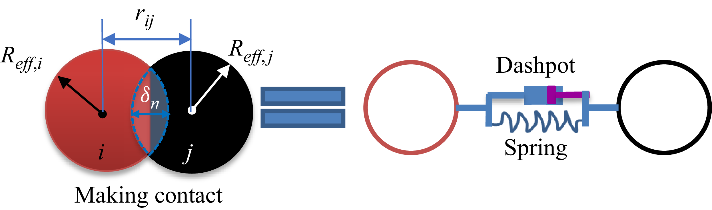
The diagram of particles making a contact.

The formulation of particle phase follows the structure of Snider’s (Reference Snider2001) MP-PIC model and a key advancement lies in replacing the particle stress closure with discrete element method (DEM) given by (2.7). The coarse-grained DEM is adopted to model particle stress for granular flows. It resolves inter-particle collisions with spring-dashpot formulations (Crowe Reference Crowe2012). As shown in (2.8), the contact model in DEM adopts the soft-sphere model. During a contact event, the interaction between two particles is modelled as the combined action of a spring and a dashpot. As illustrated in figure 1, the normal overlap
 $\delta _n$
represents the inter-particle penetration or the spring/dashpot displacement. The critical parameter governing the elastic response is the stiffness coefficient
 $k_{n,pc}$
and the displacement
 $\delta _n$
, whereas the damping effect is characterised by the damping coefficient
 $\gamma _{n,pc}$
and the relative velocity
 $\boldsymbol{v}_{r,n}$
. If the particle restitution coefficient is denoted by
 $e_{\!pc}$
, the two parameters are related through (2.9). Additionally, the drag force model proposed by McFarland’s team (Vasco et al. 2021) is applied to describe the drag coefficient
 $C_d$
, as given in (2.10). The Magnus force driven by gas rotation, which accounts for the lifting effect in compressible gas-particle systems, is given by (2.11) (Li et al. Reference Li, He, Meng and Tian2022). Here the Magnus lift coefficient
 $C_{\textit{mag}}$
equals 0.5, originally derived by Drew & Lahey (1987). In terms of the numerical scheme, a third-order Runge–Kutta method is adopted for time advancement, total variation diminishing reconstruction for left and right states and Harten-Lax-van Leer (HLL)/Harten-Lax-van Leer-Contact (HLLC) approximate Riemann solvers for flux reconstruction. Finally, model validation was performed through a case of particle curtain driven by shock, aiming to compare with the experimental results of the Rogue test (Rogue et al. 1998), as presented in figure 31 (see Appendix A).
 \begin{align}&\qquad\qquad\qquad\qquad {{\boldsymbol{A}}_{\!p,i}}=\frac {1}{{{m}_{\!p}}}\sum \limits _{j}^{}{{\boldsymbol{F}_{\textit{ji}}}}, \end{align}
 \begin{align}&\qquad\qquad\qquad \boldsymbol{F}_{ij,n} = k_{n,{\textit{pc}}}\boldsymbol{\cdot }\delta _n \boldsymbol{n} - \gamma _{n,{\textit{pc}}} \boldsymbol{\cdot }\boldsymbol{v}_{r,n}, \end{align}
 \begin{align}&\qquad\qquad\quad \gamma _{n,{\textit{pc}}} = -\frac {2\ln (e_{\!pc})}{\sqrt {\pi ^2+\ln^2 (e_{\textit{pc}})}}\sqrt {m_{\!pc}k_{n,\textit{pc}}}, \end{align}
 \begin{align}& \kappa _p = \frac {1}{8} C_d \pi d_p^2 \rho _{\!f} | \boldsymbol{{\bar u}}_{\!f} - \boldsymbol{v}_p |, \quad {\textit{Re}}_{\!p} = \frac {| \boldsymbol{{\bar u}}_{\!f} - \boldsymbol{v}_p | d_p}{\nu _{\!f}}, \nonumber\\ & C_d = \begin{cases} 18 \dfrac {{\mu} _{\!f}}{d_p^2 \rho _p} & \text{for } {\textit{Re}}_{\!p} \leqslant 0.1, \\[8pt] \dfrac {24}{{\textit{Re}}_{\!p}} \left ( \alpha _{\!f}^{-2.65} + \frac {{\textit{Re}}_{\!p}^{2/3}}{6} \alpha _{\!f}^{-1.78} \right ) & \text{for } 0.1 \lt {\textit{Re}}_{\!p} \lt 1000 ,\\[8pt] 0.424 & \text{for } 1000 \leqslant {\textit{Re}}_{\!p}, \end{cases} \end{align}
 \begin{align}&\qquad\qquad \boldsymbol{F}^{\textit{mag}}_{\!p,i}=C_{{\textit{mag}}}\rho _{\!f}(\boldsymbol{\bar u}_{\!f}-\boldsymbol{v}_{\!p,i})\times (\boldsymbol{\nabla }\times \boldsymbol{\boldsymbol{\bar u}}_{\!f}). \end{align}
3. Simulation set-up
A schematic of the numerical set-up is shown in figure 2, and both two-dimensional (2-D) and three-dimensional (3-D) cases are simulated. At the initial moment, a circular high-pressure region (part of I) mixing particles triggers a blast, generating a sequence of waves and dispersing particles under a supersonic inflow (part of II). The coupled interactions among the blast, particle dispersion and incoming flow result in a series of complex flow phenomena with significant physical implications.
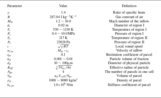
Fluid and particle parameters.

Schematic diagram of the physical flow of a particle cloud driven by pressure under supersonic inflow conditions.

The computational domain is a rectangular region of length
 $ L_x$
and width
 $ L_y$
, with free boundary conditions applied except for the inlet condition. The particle cloud is initially confined within a circular region I of diameter
 $d_c$
, filled with high-temperature and high-pressure gas. The surrounding air region II, consists of a supersonic airflow that interacts with the blast-driven shock waves, leading to more complex wave structures in the flow field. In order to investigate the effects of parameters, including particle density
 $\rho _p$
, particle diameter
 $d_p$
, inlet Mach number
 $M_{\textit{in}}$
and the driven pressure
 $P_c$
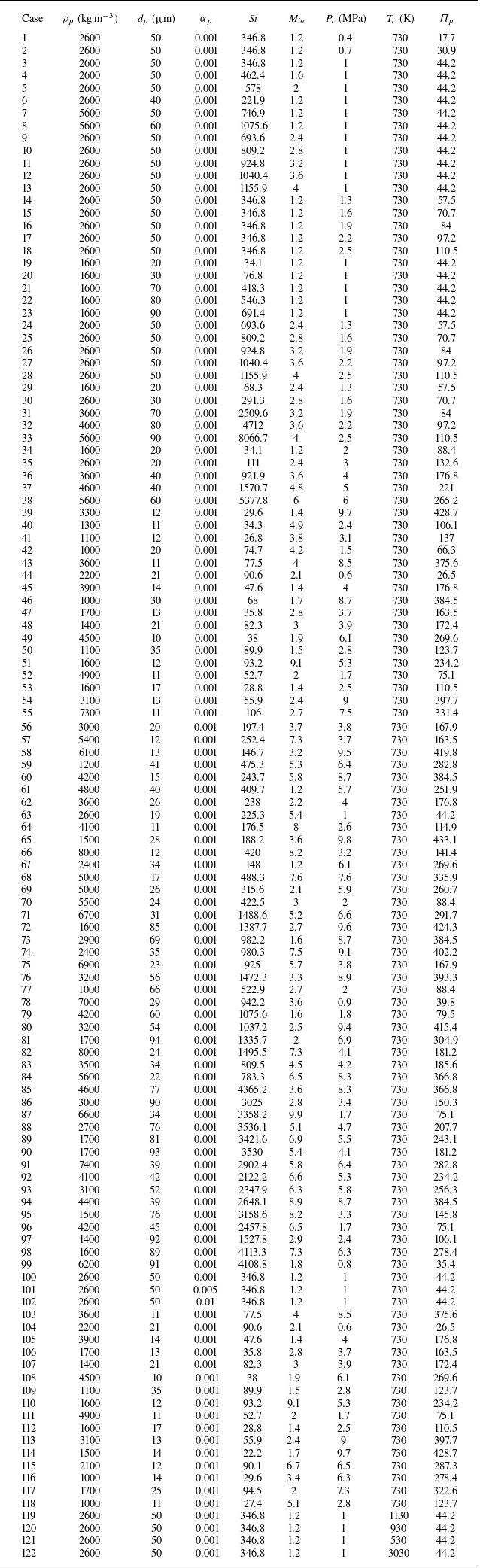
, sufficient cases are carefully designed in table 4. For all cases, the gas in the particle-laden region I is initialized at a temperature of
 $T_c$
, with an ambient pressure of 22 628 Pa and a temperature of
 $T_e$
in region II. These initial properties of the fluid and particles are detailed in table 1.
Following the blast, particles move and disperse over time, with a statistical average velocity
 $U_{m}= {1}/{N_p}\sum _{i=1}^{N_{\!p}}|\boldsymbol{v}_{\!p,i}|$
(where
 $N_p$
represents the total number of particles), forming distinct spanwise edges at positions
 $Y_{{\min}}$
and
 $Y_{{\max}}$
, as illustrated in figure 3. These edge positions can characterise the overall dispersion range. Moreover, two probes of pressure are set at 0.05 m upstream and 0.4 m downstream of the initial centre of the circle, denoted as
 $P_1$
and
 $P_2$
, respectively. Accordingly, the average velocity of particles
 $U_m$
and the probes of pressure
 $P_1$
and
 $P_2$
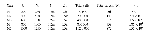
for the gas phase are selected as representative characteristic variables. A set of grid resolutions is tested to verify grid independence and minimise the influence of mesh numbers on the numerical results, as shown in table 2. The term
 $ L_{x(y)}$
represents the dimension along the X (Y) direction, while
 $ N_{x(y)}$
is defined as the number of elements along the X (Y) direction. Additionally, the total number of cells is the result of
 $N_x\times N_y$
and the total number of particles generated in region I is dependent on the grid number because of the coarse process. The coarse-graining number
 $n_{cg}$
(Brandt et al. Reference Brandt, Grabowski, Jurtz, Kraume and Kruggel-Emden2023) (i.e. the number of physical particles grouped into a single computational parcel) is considered to assess the resolution of the particle phase simulations. Here
 $2^{\textit{dim}}$
parcels (i.e.
 $N_{\!pc}$
) are put into one cell and the ‘dim’ represents the number of dimensions in the computation.
Grid-independence verification cases.

Schematic of the time evolution of a particle cloud following a blast.

Subsequently, the time evolution curves of the characteristic variables for grid resolutions are obtained from numerical simulations and the results are shown in figure 4. Except for the largest deviation, the M1 case, the other cases remain acceptable. As the grid resolution increases, the convergence trends of
 $ U_m$
,
 $ P_1$
and
 $ P_2$
can be identified. According to figure 4 and the quantitative relative error data in figure 32 (see Appendix A), the M4 case is selected as the optimal grid resolution for this study, aiming to balance sufficient efficiency and accuracy in the calculation.
Time evolution of the average velocity of particles
 $U_m$
and pressure histories recorded at 0.05 m upstream and 0.4 m downstream of the initial circle centre, denoted as
 $P_1$
and
 $P_2$
, respectively.

4. Key dimensionless parameters
The blast-inflow driven problem involves a broad range of parameters, associated with the background flow, driven conditions and particle properties, which significantly affect the flow characteristics. These parameters make it challenging to explore the potential flow law. Therefore, a set of independent dimensionless parameters is first established through dimensional analysis in this section. Subsequently, we investigate how key dimensionless numbers influence the wave kinematic characteristics, wave structures, shock–particle interactions, particle dynamics and particle morphologies.
Based on dimensional analysis, the parameters of the background flow, driven condition and particle properties can be derived into dimensionless numbers (DeMauro et al. Reference DeMauro, Wagner, DeChant, Beresh and Turpin2019; Si et al. Reference Si, Li, Meng, Wang and Tian2024). According to the three physical regions in our problem – the particle cloud, the high-temperature–pressure region and the ambient fluid – the following variables can be identified: the independent variables include
 $d_p$
,
 $\rho _p$
,
 $\alpha _p$
and
 $T_p$
for particles and
 $u_{\!\!f\infty }$
,
 $t$
(time),
 $\gamma$
,
 $R$
,
 $T_c$
,
 $T_e$
,
 $P_c$
,
 $P_e$
,
 $\rho _e$
,
 $\rho _c$
,
 $d_c$
,
 ${\mu} _{\!f}$
for the fluid. Moreover, the dependent variables cover
 $Y_{{\max}}$
,
 $Y_{{\min}}$
,
 $x_{\!p}$
,
 $|\boldsymbol{v}_r|$
(relative velocity),
 $\omega _z$
(vorticity) and
 $X_{w}$
(waves position). A total of 22 variables are considered in this system. Therefore, four fundamental units (
 $\rho _e, u_{\!f\infty },d_c,T_e$
) selected as basic variables can derive 18 dimensionless numbers by Buckingham theory. Applying the equation of state for an ideal gas and equivalent transformation (see Appendix A.1), the simplified parameters can be defined as
 \begin{equation} \begin{aligned} \varPi _p &=\frac {P_c}{P_e}; \quad \pi _3 = \frac {T_c}{T_e} ; \quad {\textit{Re}}_{\!g} = \frac {\rho _e u_{\!f\infty } d_c}{{\mu} _{\!f}}; \quad M_{\textit{in}}=\frac {u_{\!f\infty }}{\sqrt {\gamma\! \textit{RT}_e}} ; \quad \pi _7 = \frac {d_p}{d_c};\\ \pi _8 &= \frac {\rho _p}{\rho _e}; \quad \pi _9 = \frac {T_p}{T_e}; \quad t^*= \frac {t \boldsymbol{\cdot }u_{\!f\infty }}{d_c} ; \quad Y_{{\max}}^* = \frac {Y_{\max }}{d_c} ; \quad Y_{{\min}}^* = \frac {Y_{\min }}{d_c} ;\\ X_p^* &= \frac {X_p}{d_c}; \quad {\pi _{14}={\textit{Re}}_{\!p};} \quad w_z^* = \frac {\omega _z d_c}{u_{\!f\infty }}; \quad X_w^* = \frac {X_w}{d_c}; \quad \pi _{18}=\alpha _p . \end{aligned} \end{equation}
As a result, depending on a total 15 dimensionless numbers (eliminating the redundant
 $\pi _1$
and
 $\pi _5$
, without considering the gas constant
 $\gamma$
), the system can be expressed as
 $f(\varPi _p, \pi _3, \ldots , X_w^*, \alpha _p) = 0$
. The dimensionless parameter group considered in this study is relatively large, and thus, it is necessary to simplify the parameters under quasi-steady conditions. The parameter
 $\pi _9$
represents the ratio of the particle temperature to the environment temperature. Based on the interphase heat transfer model, the simplified expression of the temperature variation rate and the thermal relaxation time ((A13), (A14), (A15)), the dimensionless thermal relaxation time can be defined as
 \begin{align} \frac {\tau _T}{\tau _{\!f}} = \frac {\alpha _{\!f} \rho _{\!f} C_v V_{\!pc} u_{\!f\infty }}{\alpha _p \textit{Hd}_c} ,\end{align}
where
 $H$
denotes the heat transfer coefficient between the particle and gas. From the estimation of magnitude order (see Appendix A), the order of
 $ {\tau _T}/{\tau _{\!f}}$
is approximately
 $10^{4}$
, which is
 $ \gg 1$
. This indicates that the particle temperature can be regarded as quasi-steady in the flow field. Therefore, the effect of
 $ \pi _9$
can be neglected.
However, the Stokes number
 ${\textit{St}} = {\rho _p d_p^2 u_{\!f\infty }}/{18 {\mu} _{\!f} d_c}$
, which can be transformed into
 $ {\pi _8 \pi _7^2}/{18} ({\textit{Re}}_{\!g})$
. This indicates that
 ${\textit{St}}$
is a combined dimensionless group involving
 $\pi _8$
,
 $\pi _7$
and
 ${\textit{Re}}_{\!g}$
. Thus,
 ${\textit{St}}$
can still be used to represent their collective influence in the subsequent study, while it should be clarified which parameter (i.e.
 $\pi _7$
,
 $\pi _8$
or
 ${\textit{Re}}_{\!g}$
) variation primarily leads to the change in
 ${\textit{St}}$
. In addition, we prefer to apply the combined
 ${\textit{St}}$
to describe the significant particle–gas interaction because
 ${\textit{Re}}_{\!g}$
only includes variables of the pure gas phase. Furthermore,
 ${\textit{St}}$
can characterise the particle’s inertial response and ability to follow the fluid. Here
 $M_{\textit{in}}$
reflects compressibility effects, controlling shock formation and propagation;
 $\varPi _p$
represents the blast intensity, determining shock speed and energy release rate. The ratio
 $ {T_c}/{T_e}$
affects the sound speed at the explosion centre, which may alter the wave velocity. Additionally,
 $t^*$
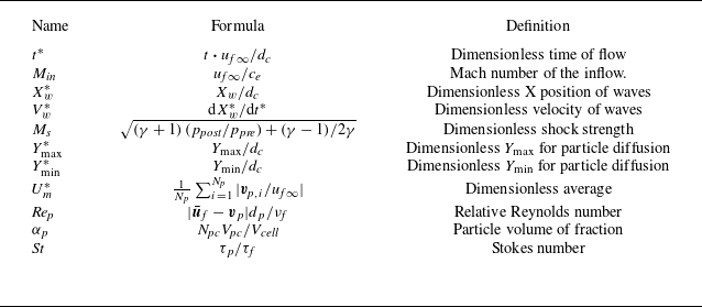
spans the entire unsteady process and captures the flow evolution. The flow problem can be decomposed into vortex generation, shock dynamics and particle dynamics, leading to the function given in (4.3) (some detailed definitions and physical significance of parameters in this study are summarised in table 3):
 \begin{equation} \begin{aligned} f\bigg( \varPi _p,\frac {T_c}{T_e},\textit{St},M_{{\textit{in}}}, \frac {d_p}{d_c},\frac {\rho _p}{\rho _e},\alpha _p, t^*;\,\, Y_{{\textit{max}(\textit{min})}}^*, X_p^*,{\textit{Re}}_{\!p},X_w^*\ldots \bigg)=0 .\end{aligned} \end{equation}
Dimensionless numbers, their calculation formulas and physical significance.

Overall, dimensionless parameters named
 $ \varPi _p, {T_c}/{T_e},St,M_{\textit{in}}, {d_p}/{d_c}, {\rho _p}/{\rho _e}$
,
 $\alpha _p$
are considered as the control parameters (initial conditions) in our study, while the other dimensionless parameters derived by dependent variables are investigated in the results section. Considering the broad parameter space of this study, the preliminary discussions on the two parameters,
 $ {T_c}/{T_e}$
and
 $\alpha _p$
, are provided in Appendices A.4 and A.5. A more detailed analysis will be conducted in future work. In terms of case setting, eight cases (cases 1–8) are preliminarily designed to investigate the effects of these parameters. Specifically, cases 1–3 examine the influence of
 $\varPi _p$
, then cases 3–5 vary
 $M_{\textit{in}}$
. Moreover, cases 6–8 and case 3 focus on the influence of particle properties (
 $\rho _p$
or
 $d_p$
), resulting in modified
 ${\textit{St}}$
on particle dynamics. Here we have simulated more than 100 cases, detailed settings of which are provided in table 4.
Variable parameters of all cases.

5. Results and analysis
For this blast–inflow–driven problem, rapidly evolving waves strongly affect the dynamic and thermal states, while the particles respond to these changes, resulting in complex wave–particle interaction and diverse flow behaviours. Since the results contain extensive content, we briefly outline the research focus and logic of each subsection as follows.
-
(i) Section 5.1 presents the fundamental wave structures, types and vortex-related analysis in the blast–inflow system.
-
(ii) The motion characteristics of these waves, including the main shock, SecS and contact surface, are analysed parametrically in § 5.2.
-
(iii) In addition, the present problem involves a gas–particle system, where the interactions between the waves and particles are non-negligible, as discussed in § 5.3.
-
(iv) Finally, § 5.4 investigates the particle forces, dispersion dynamics and the resulting dispersion morphologies.
5.1. Wave structures
In order to investigate the temporal evolution of wave structures in this blast-inflow driven problem, we plotted a numerical schlieren image, shaded by the streamwise component
 $\boldsymbol{\nabla} _x\rho$
, which allows for a clearer observation of the complex wave structures. Several representative snapshots are presented in figure 5. The gas-phase data, including density
 $ \rho _{\!f}$
, pressure
 $ P_{\!f}$
and streamwise velocity
 $ u_{\textit{fx}}$
, are extracted along the Xdirection at the centreline
 $Y = {L_y}/{2}$
. Here the magnitude of the particle velocity,
 $| \boldsymbol{v}_p |$
, is visualised using contour plots to illustrate the velocity variation of the particle cloud.
Numerical result for
 $\boldsymbol{\nabla} _x P_{\!f}$
, X-
 $u_{\textit{fx}}$
and X-
 $P_{\!f}$
plots along the centreline
 $Y = {L_y}/{2}$
, where (a) to (h) correspond to the time sequence: 0.03, 0.09, 0.18, 0.27, 0.45, 0.60, 0.99 and 1.77 ms.

The evolution of wave structures exhibits a sequence of distinct stages, governed by the interplay between the outward blast, the incoming flow and the particle interactions. Initially, the flow resembles a classical outward blast, including the leftmost (rightmost) main shock (L(R)MS). As shown in figures 5(a) and 5(b), the early stage of the computation resembles a pure outward blast, featuring a bow-shaped main shock and a contact surface. The values of
 $ u_{\textit{fx}}$
and
 $ P_{\!f}$
remain continuous behind the main shock, but the density gradient exhibits discontinuities, indicating the presence of a contact surface. As shown in panels (c) and (d), the particle cloud remains at a lower velocity than the contact surface, allowing the contact surface to pass through the particle cloud. In this region, panel (c) highlights the implosion process induced by radial over-expansion (Ling & Balachandar Reference Ling and Balachandar2018a
,
Reference Ling and Balachandarb
), as the lowest pressure
 $ P_{\!f}$
approaches vacuum levels and pressure discontinuities appear on both sides. This provides the condition for implosion, the SecS forming at the tail of the expansion fan (Friedman Reference Friedman1961), then converging to a centre point (Prentice Reference Prentice1968). In panel (d) the initiation of an outward SecS is captured after the converging process. After the contact surface traverses the particle cloud, the inflow velocity
 $ u_{\textit{fx}}$
reaches approximately 300 m s−1, leading to the emergence of a detached shock, as shown in panel (e). At this moment, the SecS coincides with the contact surface. In panels (f) and (g), the SecS continues to propagate outward after impinging the contact surface, which is in perfect agreement with RMIs (Ling et al. Reference Ling, Wagner, Beresh, Kearney and Balachandar2012; Ling & Balachandar Reference Ling and Balachandar2018a
). In a typical RMI, a shock interacts with a pre-existing density interface. Here, the SecS acts as the shock, while deformed contact surface (DCS) serves as the density interface, satisfying the conditions for RMI formation. Moreover, DCS allows tangential velocity shear (i.e. a characteristic of the contact surface; see figure 33 in Appendix A) especially under inflow conditions, jointly contributing with the RMIs to vorticity generation and deposition. In panel (h) a relative velocity exists between the particle cloud and the DCS. Over time, the DCS gradually moves away from the particle cloud and begins to curl, eventually evolving into the classical ‘cat’s eye’ vortex. Meanwhile, the SecS continues to propagate through the particle cloud, which may trigger SDMI.
Schematic wave structures in outward blasts driven by different conditions. (a) Typical wave pattern in a shock or blast-driven blast. (b) Instantaneous wave structure in a blast-inflow driven problem. (c) A
 $x$
-time diagram of waves along the centreline
 $y = {L_y}/{2}$
for a blast-inflow driven problem. Here UPF and DPF denotes upstream and downstream particle front, respectively.

Previous research has commonly approximated the early stage of gas–particle blasts in static environments as spherical shock-tube problems, which generate some typical wave structures. Ling et al. (Reference Ling, Haselbacher and Balachandar2011b
) summarised these typical wave structures, including the outermost main shock, the contact surface (discontinuity), the SecS and the inward-propagating rarefaction fan, as illustrated in figure 6(a). However, these typical wave structures may deform on the impact of particles and supersonic inflow in present blast-inflow driven problems, as shown in figure 6(b). Because of this deformation, describing the evolution of wave structures can be more complex. Thus, an
 $x{-}t$
diagram is plotted in figure 6(c) to consider the time effects and validate the wave patterns corresponding to figure 5 by extracting data along the midline at
 $Y = {L_y}/{2}$
. Overall, the two types of problems exhibit distinct differences in the morphology and evolution of wave structures. In the case of shock or blast-driven blasts, particle–wave interactions occur primarily during the initial stage of the blast. In contrast, for the blast-inflow driven type, such interactions may persist throughout the entire process, involving not only the blast-induced wave system but also the detached shock formed ahead of the particle front.
Notably, the identified vortex deposition is closely related to the SecS impinging on the DCS, which can be classified as a RMI. Therefore, we focus on the quasi-steady vortex structures since the deposited vortex evolves into large eddies over time.
In order to investigate the influencing factors of vorticity dynamics evolution, the inviscid compressible multiphase vorticity dynamics equation is given as
 \begin{equation} \begin{aligned} \frac {D \omega _z}{D t} &= - \omega _z (\boldsymbol{\nabla }\boldsymbol{\cdot }\boldsymbol{u}_{\!f}) + \frac {\boldsymbol{\nabla }\!\rho _{\!f} \times \boldsymbol{\nabla }\!p_{\!f}}{\rho _{\!f}^2} + \boldsymbol{\nabla }\times \left ( \frac {\boldsymbol{S}_{\textit{mp}}}{\alpha _{\!f}\! \rho _{\!f}} \right ) ,\\ \boldsymbol{S}_{\textit{mp}} &= \frac {1}{V_{\textit{cell}}} \sum _i \kappa _{\!p,i} (\boldsymbol{v}_{\!p,i} - \boldsymbol{u}_{\!f}), \end{aligned} \end{equation}
The spatial distribution contour plots of vorticity.

where the terms
 $(\boldsymbol{\omega } \boldsymbol{\cdot }\boldsymbol{\nabla })\boldsymbol{u}_{\!f}$
,
 $\boldsymbol{\omega }(\boldsymbol{\nabla }\boldsymbol{\cdot }\boldsymbol{u}_{\!f})$
,
 $ {\boldsymbol{\nabla }\!\rho \times \boldsymbol{\nabla }\!p}/{\rho ^2}$
and
 $\boldsymbol{\nabla }\times ( {\boldsymbol{S}_{\textit{mp}}}/{\alpha _{\!f}\! \rho _{\!f}} )$
are the vorticity stretching term, volumetric expansion (compression) term, baroclinic term and the drag force rotation term, respectively. This equation describes the evolution of vorticity due to velocity gradients, flow compressibility and baroclinic flow effects. Here the vorticity stretching term can be expressed as
 $(\boldsymbol{\omega } \boldsymbol{\cdot }\boldsymbol{\nabla })\boldsymbol{u}_{\!f} = 0$
in 2D flow (Lee Reference Lee1951); thus, the time evolution of vorticity is mainly related to the divergence term and the baroclinic term. In contrast to the vorticity deposition caused by SDMI (Black et al. Reference Black, Denissen and McFarland2018), the vorticity core lies completely outside of the shear layer, and there is still a vorticity deposition that has Not spiral shape (NSS, also originally part of DCS; see, e.g., figure 5
g) at
 $t = 2.34 \, \text{ms}$
shown in figure 7. The vorticity changes are most concentrated in the curled DCS near the vortex core, shear layer and NSS region, because the DCS has a strong density discontinuity surface and the SecS has a large pressure gradient. If the gradients are no longer collinear, i.e.,
 ${\boldsymbol{\nabla }\!\rho _{\!f} \times \boldsymbol{\nabla }\!p_{\!f}} \neq 0$
, vorticity will be generated and deposited with time evolution. Moreover, the contact surface (e.g., DCS and NSS) allows tangential velocity discontinuity, leading to velocity shear, which also contributes to vorticity generation and deposition. This helps explain the curling phenomenon of the DCS shown in figure 5(h): its shape is no longer a regular circle due to the lag of the cloud, and the shear of velocity exists in the tangential direction, providing conditions for vorticity generation.
Compared with the governing equation given in a study (McFarland et al. Reference McFarland, Black, Dahal and Morgan2016), the viscous dissipation term
 $\nu \boldsymbol{\nabla} ^2 \omega$
is neglected here, but the influence of the volumetric expansion term
 $\boldsymbol{\omega } (\boldsymbol{\nabla }\boldsymbol{\cdot }\boldsymbol{u}_{\!f})$
and particle source term
 $\boldsymbol{\nabla }\times {\boldsymbol{S}_{\textit{mp}}}/{\alpha _{\!f}\!\rho _{\!f}}$
is considered. Figure 8 shows the corresponding divergence and baroclinic terms at the same time to assess their impact on vorticity evolution. Although the maximum magnitude of
 $\boldsymbol{\omega } (\boldsymbol{\nabla }\boldsymbol{\cdot }\boldsymbol{u}_{\!f})$
is about
 $10^{-1}$
of
 $ {\boldsymbol{\nabla }\!\rho _{\!f} \times \boldsymbol{\nabla }\!p_{\!f}}/{\rho _{\!f}^2}$
, the value out of the vortex core cannot be neglected. For example, NSS is spatially located between the shear layer and the DCS influenced not only by the evolution of the DCS, but also by its continuous interaction with the shear layer of velocity.
The spatial distribution contour plots of the baroclinic term (a) and the divergence term (b) at t = 2.34 ms.

5.2. Wave motion
Furthermore, examining the characteristics of wave motion provides insight into the position, propagation velocity and intensity of these waves. However, the evolution of the shapes of the L(R)MS, DCS and SecS is highly complex and eventually becomes irregular. Therefore, only the wave characteristics along the centreline
 $Y = {L_y}/{2}$
are analysed for clarity.
For supporting quantitative data of these waves, we denote the dimensionless position
 $X_w^*$
for L(R)MS, SecS and DCS-left (DCSL) as
 $X_{\textit{SL(R)}}^*,X_{\textit{SSL(R)}}^*\, \text{and}\,X_{\textit{DCSL}}^*$
and the corresponding dimensionless velocity as
 $V_{\textit{SL(R)}}^*,V_{\textit{SSL(R)}}^*\, \text{and}\,V_{\textit{DCSL}}^*$
, as given in (5.2):
 \begin{equation} V_w^* = \frac {{\rm d} X_w}{u_{\!f\infty } \boldsymbol{\cdot }{\rm d}t} ,\end{equation}
The shock Mach number of the L(R)MS and SecS is denoted by
 $M_{\textit{SL(R)}},M_{\textit{SSL(R)}}$
and can be calculated using
 \begin{equation} Ms= \sqrt { \frac {(\gamma + 1)\, (p_{\textit{post}}/p_{\textit{pre}}) + (\gamma - 1)}{2\gamma } },\end{equation}
The dimensionless position, velocity and shock Mach number of waves as a function of
 $t^*$
for case 3.

where the sound speed ahead of the shocks satisfies
 $c_{\textit{pre}} = \sqrt {\gamma p_{\textit{pre}}/\rho _{\textit{pre}}}$
. Here the subscript ‘pre’ and ‘post’ represent the unshocked and shocked state, respectively. Dimensionless time can be defined as
 $t^*={u_{\!f\infty }t}/{d_c}$
.
As shown in figure 9(a), the leftmost main shock (LMS) moved upstream early and then moved downstream at approximately
 $t^* = 13.3$
. Accordingly, the condition
 $V_{\textit{SL}}^* = 0$
occurs at
 $t^*=13.3$
. This transition is attributed to the radial over-expansion, which initially drives the LMS upstream, followed by a downstream motion to accommodate the decreasing back pressure (see the decreasing post-shock pressure in figure 5
d–e), the curve of
 $P_{\!f}-x$
. For the rightmost main shock (RMS), it has similar characteristics to the LMS. For
 $t^* \lt 6.3$
, the rate of decrease of
 $V_{\textit{SL(R)}}^*$
and
 $M_{\textit{SL(R)}}$
is relatively large. But when
 $t^* \gt 6.3$
, the rate of decrease slows down and eventually converges. Overall, both
 $V_{\textit{SL(R)}}^*$
and
 $M_{\textit{SL(R)}}$
exhibited a power-type decay with time: they decrease rapidly at early times and gradually approach a constant value.
As mentioned earlier, the SecS converges inward due to the implosive environment and then propagates outward (see figure 5
c–d). During its outward motion, it passes through the DCS, with the intersection points marked by a yellow circle in figure 9(a). In terms of velocity and intensity, both the L(R)MS and SecS exhibit significant variations once the blast is released. Specially, the SecS exhibits a stronger intensity during its convergence in the early stage in panel (c), and subsequently exhibits a decay trend after the converging process (i.e. the SecS propagates outward). However, both shocks show only minor variations in the long-term evolution. As for the DCSL, it is mainly accelerated by the post-wave gas flow; therefore, its velocity cannot exceed the incoming flow velocity, i.e.
 $V_{\textit{DCSL}}^*\lt 1$
. In addition, since the DCSL is not a shock, it has no shock-strength parameter.
5.2.1. Main shock
Subsequently, in the multi-case results, the motion and intensity evolution of the L(R)MS are shown in figure 10. In panels (a–c) the curves of cases 3 and 6–8 collapse, indicating that
 ${\textit{St}}$
(altered by
 $d_p$
and
 $\rho _p$
) has negligible influence on the L(R)MS dynamics in this parameter space. Here
 $\varPi _p$
introduces some variations during the blast stage, but has limited impact on the subsequent steady evolution for the main shock. In contrast, comparison of cases 4 and 5 reveals that variations in
 $M_{\textit{in}}$
have a pronounced impact on
 $X_{\textit{SL(R)}}^*$
,
 $V_{\textit{SL(R)}}^*$
and
 $M_{\textit{SL(R)}}$
, with higher
 $M_{\textit{in}}$
enhancing both velocity and strength of the LMS. In addition, fluctuations can be observed in the velocity of the shock front, as marked in figure 10(b), and a similar fluctuation behaviour is also found in the shock strength shown in panel (c). In general, such short-term fluctuations are not expected in the evolution of a blast wave. However, in the present gas–particle coupled system they can indeed occur, particularly due to the shock–particle interactions. These interactions at the same
 $t^*$
, discussed in detail in § 5.3, are identified as the primary cause of the observed variations.
Wave kinematic characteristics for multiple cases along the centreline at
 $Y = {L_y}/{2}$
for L(R)MS. (a) Wave position as a function of time. (b) Wave velocity as a function of time. (c) Wave strength as a function of time. (d) Wave radius as a function of time in logarithmic coordinates.

In a strong point-source explosion, the well-known scaling law between the shock radius and time is given by
 $r_s\propto t^{({2}/{N+3})}$
(
 $N=0$
, 1, 2 represents planar, cylinder and sphere blast, respectively). However, the present problem involves a finite-size blast interacting with an inflow, which differs fundamentally from the idealised point-source explosion scenario. Moreover, the blast strength in our study is considerably weaker than nuclear-scale explosions where such scaling laws are typically observed. Given these differences, it is unclear whether any relationship exists for the main shock evolution with time in our configuration. To investigate this question empirically, we plot the dimensionless shock radius and time curves for cases 1–8 in figure 10(d). Here, an effective shock radius is defined as
 $r_s^*= {(X_{\textit{SR}}^*{-}X_{\textit{SL}}^*)}/{2}$
, which characterises the effective propagation range rather than implying circularity of the blast wave.
The results suggest that, within certain limitations, the relationship between
 $r_s^*$
and
 $t^*$
can be approximately described by a power-law form
 $r_s^*\propto t^{*q}$
. The fitted exponents
 $q$
for different cases are listed in table 5 (see Appendix A). However, it is important to emphasise that this approximate power-law behaviour is subject to two main factors: (i) shock–particle interactions, as discussed in § 5.3, particularly when the LMS overtakes the particle cloud, introduce fluctuations in velocity and strength; (ii) even in the absence of particle interactions, the main shock undergoes gradual decay as it propagates, which inherently weakens the power-law relationship. As noted by Ling & Balachandar (Reference Ling and Balachandar2018a
), asymptotic decay effects become increasingly important at later times.
The exponent of the power-law fitting for the dimensionless shock radius to time (
 $r_s^*$
to
 $t^*$
) for cases 1–8.

5.2.2. Secondary shock and contact surface
The SecS is generated in the tail of the expansion wave in an implosion environment with a weak strength and initially follows outward (figure 9 c). As the implosion converges, the shock intensity increases rapidly, reaching its maximum at the convergence point, where it reflects and subsequently propagates outward, decreasing and eventually stabilising the strength. Considering multiple cases for SecS and DSC, the dimensionless positions, velocities and strengths of the waves are illustrated in figures 11, 12 and 13.
The dimensionless position of waves as a function of
 $t^*$
for cases 1–8.

The dimensionless velocity of waves as a function of
 $t^*$
for cases 1–8.

The Mach number of SecS as a function of
 $t^*$
for cases 1–8.

Case 1–8 indicate that the SecS undergoes a convergence process. In addition, the SecS impinges on the DCSL, with the intersection points marked by coloured circles, as shown in figure 11. The results show that both the convergence position and convergence time of the SecS increase with
 $\varPi _p$
(figure 11
a). Similarly, the impinged position and time of the DCSL also exhibit an increasing trend. According to the moving planar shock relationship developed from Rankine–Hugoniot (DRC
 $\gt$
0, i.e. the shock moves positively):
 \begin{align} V_{\textit{post}}=V_{\textit{pre}}+\text{sign(DRC)}\boldsymbol{\cdot }c_e\frac {2(p_{\textit{pre}}/p_{\textit{post}}-1)}{\sqrt {2\gamma [(\gamma +1)p_{\textit{pre}}/p_{\textit{post}}+\gamma -1]}}, \end{align}
a stronger pressure release produces higher radial velocity initially. As a result, the SecS remains convected outward for a longer time, leading to a larger diameter. This is confirmed in figure 11(a), cases with larger
 $\varPi _p$
show greater diameters (
 $ D_{\textit{SS}}^* = X_{\textit{SSR}}^* - X_{\textit{SSL}}^*$
) of the SecS in an instant
 $ t^*$
. This also explains why the SecS in case 1 (figure 12
a) shows an earlier velocity change, i.e. the weaker radial flow causes a shorter following time and, hence, earlier convergence. A similar trend is observed in the SecS strength, which converges earlier. Furthermore, the peak of
 $M_{\textit{SS}}$
increases with
 $\varPi _p$
(figure 13
a).
However, when
 $\varPi _p$
is fixed but
 $M_{\textit{in}}$
increases (figure 11
b), the SSL stands for SecS-left is nearly insensitive to
 $M_{\textit{in}}$
. Increasing
 $M_{\textit{in}}$
inevitably enhances the post-velocity of the LMS, while the SSL experiences a stronger blow, which explains the pronounced sensitivity of the SSL to
 $M_{\textit{in}}$
. The dimensionless SecS velocity
 $V_{\textit{SS}}^*$
, defined as the ratio of the SecS velocity to the inflow, is relatively smaller in case 5 with the largest
 $M_{\textit{in}}$
(figure 12
b), indicating that the SecS velocity increases more slowly than the inflow velocity. In terms of intensity, the peak strength of
 $M_{\textit{SS}}^*$
occurs at a larger
 $t^*$
with increasing
 $M_{\textit{in}}^*$
(figure 13
b). This indicates that a longer characteristic time is required for the SecS to reach its maximum strength. Moreover, the results suggest that changing only
 $d_p$
and
 $\rho _p$
within the limited range of variations may not noticeably affect the wave dynamics (see figures 11
c, 12
c and 13
c).
5.3. Interactions among waves and particle cloud
In this section we focus on representative interaction scenarios involving the LMS, SecS, DCS and particle cloud, as well as their effects and the key factors that promote these interactions, such as elevated
 $M_{\textit{in}},St$
.
As established in § 5.2.1, the velocity and strength of the L(R)MS are highly sensitive to variations in the inflow Mach number
 $M_{\textit{in}}$
. Moreover, local fluctuations are observed in figure 10(b,c), where the approximate power-law scaling of
 $r_s^*$
with
 $t^*$
in cases 4 and 5 is also affected, as shown in figure 10(d). To explore the influence of
 $M_{\textit{in}}$
on wave structures, wave motion and the approximate scaling law, contour plots of
 $ {\partial \rho _{\!f}}/{\partial x}$
at several representative dimensionless times
 $t^*$
are presented for cases 3–5 in figure 14.
Schlieren images of
 $ {\partial \rho _{\!f}}/{\partial x}$
for cases 3–5 at four typical dimensionless times
 $t^*$
.

The results reveal two key phenomena. First, the NSS plays a critical role as a transitional structure between DCS and the vortex. As discussed in § 5.1, the NSS is simultaneously influenced by both the shear layer and DCS, which may induce structural modifications. At low
 $M_{\textit{in}}$
, the NSS tends to decouple from the DCS and forms a secondary vortex (case 3,
 $t^*=53.15$
), whereas at high
 $M_{\textit{in}}$
, the NSS is more effectively absorbed by the DCS or vortex core, as demonstrated in cases 3–5 at
 $t^* = 53.15$
. Second, the particle lag relative to the LMS plays an important role in promoting shock–particle interaction. Specifically, increasing
 $M_{\textit{in}}$
enhances the interaction between the main shock and the particle cloud. Because
 $|\boldsymbol{v}_p| \lt |V_{\textit{SL}}|$
, the distance between the particle cloud and the LMS gradually decreases. In case 4 the detached shock behind the cloud intersects and merges with the LMS, as shown in figure 14. Due to the stronger lag in case 5, the LMS continuously compresses the particle cloud, which deforms from an elliptical to a compressed crescent shape. During this interaction, the LMS transitions from a bow shock to a parabolic shock and eventually resembles an oblique shock near the flanks. These shock–particle and shock–shock interactions explain the fluctuations in
 $V_{\textit{SL(R)}}^*$
and
 $M_{\textit{SL(R)}}$
observed in figure 10(b,c) at
 $t^*\approx 23.39$
. The LMS-detached shock merging and continuous cloud compression jointly contribute to these fluctuations and affect the approximate power-law scaling of
 $r_s^*$
with
 $t^*$
shown in figure 10(d).
Furthermore, the LMS may also impinge directly through the particle cloud. Based on the preceding analysis, increasing
 $M_{\textit{in}}$
causes the LMS to propagate more rapidly downstream. Meanwhile, the cloud possesses a long relaxation time and exhibits significant lag due to its extremely large Stokes number (
 ${\textit{St}} = 8066.7$
at
 $M_{\textit{in}}=4.0$
in case 33). Consequently, higher
 $M_{\textit{in}}$
and
 ${\textit{St}}$
enable the LMS to impinge through the cloud, as illustrated in figure 15.
Diagram of a highly lagged particle cloud directly impinged by the LMS in case 33. (a) The LMS has just impinged through the cloud at
 $t^*=14.2$
. (b) Post-impingement evolution of the cloud and waves at
 $t^*=35.5$
. The magnitude of the density gradient
 $|\boldsymbol{\nabla }{\rho }|$
and
 $u_{\textit{fx}}$
are used to plot the contour and contour lines, respectively.

In figure 15(a) the particle cloud lags behind the LMS and is just being impinged, leaving the cloud fully exposed to the background flow. In panel (b) the distance between the cloud and LMS increases due to lag effects. Two oblique shocks subsequently appear above and below the cloud, driven by the sustained background flow. These observations indicate that excessive lag modifies the relative configuration between the cloud and LMS, thereby promoting their interaction. Additionally, the results demonstrate that the SSL may interact with the SSR stands for SecS-right at elevated
 $M_{\textit{in}}$
. Panel (a) shows the convergence of the SecS, with contour lines plotted by the post-shock velocity
 $u_{\textit{fx}}$
. The exceedingly high velocity contributes to a pronounced deformation of the SecS. Consequently, it is necessary to treat the SecS as two separate shocks (a normal SSL and a curved SSR). The intrinsic intersection at the top and bottom triggers a shock–shock interaction in the supersonic flow, producing a complex derivative-wave system (so-called regular reflection or Mach reflection; see Baby, Paramanantham & Rajesh 2024), as illustrated in panel (b).
Figure 15 has illustrated the main shock–particle interaction at an extremely large
 ${\textit{St}}$
. In contrast, a cloud with a small Stokes number (
 ${\textit{St}}=29.6$
, case 39) may interact continuously with the DCS, as shown in figure 16. In panel (a) a remarkable difference in the post-shock velocity
 $u_{\textit{fx}}$
of the SecS is still observed (including figures 15
a and 5
c). This difference originates from opposite propagation directions during convergence. The post-shock velocity of the SSL can even exceed
 $u_{\!f\infty }$
. Consequently, a portion of the particles with smaller
 ${\textit{St}}$
is entrained by the high-speed region, interacting with the DCS or forming a particle jetting, as illustrated in figure 16(b).
Diagram of the particle cloud interacting with the SecS and DCS for case 39. (a) The SecS converges inward and interacts with the particle cloud at
 $t^{*}=9.2$
. (b) A portion of the particle cloud interacts with DCS at
 $t^{*}=41.5$
. The magnitude of the density gradient
 $|\boldsymbol{\nabla }\!\rho |$
and
 $u_{\textit{fx}}$
are used to plot the contour and contour lines, respectively.

Overall, the interactions among the LMS, SecS, DCS and particle cloud are governed by their relative velocities and positions. Increasing
 ${\textit{St}}$
and
 $M_{\textit{in}}$
causes the LMS to migrate toward and compress the cloud; if penetration occurs, the cloud becomes fully exposed to the supersonic free stream. The SecS impinges through the cloud twice: during convergence, particles may be entrained into jets; after reflection, it interacts with the DCS, triggering RMI. The DCS–cloud interaction depends critically on the relative position: at high relative velocity, the DCS passes through the cloud with deformation; at low relative velocity, the cloud experiences continuous velocity shear and vortex entrainment. However, when the cloud stays upstream of the DCS without entering the vortex region, particles at the periphery are decelerated by the low-velocity zone of the vortex pair (figure 5
h), leading to erosion.
The relative displacement
 $Rd$
can serve as a criterion for characterising these interactions, as expressed in (5.5):
 \begin{equation} \begin{aligned} Rd ^{p,i}_{w(t)}=\int _0^t(V_w-V_{\!p,i}){\rm d}t,\\ Rd ^{w'}_{w(t)}=\int _0^t(V_w-V_{w'}){\rm d}t .\end{aligned} \end{equation}
Here
 $\textit{Rd}$
is a function of time
 $t$
, where the subscript (or superscript)
 $p,i$
denotes the particle
 $i$
,
 $w$
represents the waves (LMS, RMS, SSL, SSR or DCS) and
 $w'$
indicates a different wave type. If
 ${\textit{Rd}}_{(t_0)}=0$
at
 $t=t_0$
, the two entities intersect and interact. Furthermore, if
 ${\textit{Rd}}_{(t_0^-)}\boldsymbol{\cdot } {\textit{Rd}}_{(t_0^+)}\lt 0$
, they penetrate each other; if
 ${\textit{Rd}}_{(t_0^-)}\boldsymbol{\cdot } {\textit{Rd}}_{(t_0^+)}\approx 0$
, sustained interaction occurs; if
 ${\textit{Rd}}_{(t_0^-)}\boldsymbol{\cdot } {\textit{Rd}}_{(t_0^+)}\gt 0$
, they separate after interaction (analogous to collision). Future work may focus on investigating the explicit functional form of
 $V_{w(p)}=f( \varPi _p, ({T_c}/{T_e}),St,M_{{\textit{in}}}, ({d_p}/{d_c}),({\rho _p}/{\rho _e}), t^*\ldots )$
.
5.4. Particle motion
The evolutionary motion of particles is governed by various forces, determining the characteristics of dispersion. The cloud exhibits distinct features in spanwise dispersion and overall morphologies. Accordingly, this section investigates the forces acting on particles, dispersion dynamics and the resulting morphologies.
5.4.1. Forces acting on particles
This subsection focuses on the forces acting on particles, including collision force, drag force, Magnus force and gradient force, which play a crucial role in particle dynamics.
Distribution of
 $|\boldsymbol{a}_{col}^*|_{{avg}}$
,
 $|\boldsymbol{a}_{\textit{drag}}^*|_{{avg}}$
,
 $|\boldsymbol{a}_{\boldsymbol{\nabla }P_{\!f}}^*|_{{avg}}$
and
 $|\boldsymbol{a}_{\textit{mag}}^*|_{{avg}}$
as a function of
 $t^*$
.

In particle dynamics, the temporal evolution of forces determines the particle motion, where the forces can be related to corresponding accelerations, as shown in (5.6):
 \begin{equation} \boldsymbol{a}_{\!p,i}=\boldsymbol{a}_{\textit{drag},i}+\boldsymbol{a}_{\boldsymbol{\nabla }P_{\!f},i}+\boldsymbol{a}_{\textit{mag},i}+\boldsymbol{a}_{\textit{col},i}. \end{equation}
The accelerations
 $\boldsymbol{a}_{col}$
,
 $\boldsymbol{a}_{\textit{drag}}$
,
 $\boldsymbol{a}_{\textit{mag}}$
and
 $\boldsymbol{a}_{\boldsymbol{\nabla }P_{\!f}}$
correspond to collision, drag, Magnus and pressure-gradient forces, respectively, and are non-dimensionalised as
 $\boldsymbol{a}^* = \boldsymbol{a} \boldsymbol{\cdot }d_c/u_{\!f\infty }^2$
. Given the large number of particles, we employ statistical averaging, i.e.
 \begin{equation} {\eta _{{avg}}=\frac {1}{N_p}\sum _{i=1}^{N_{\!p}}\eta _n^i}, \end{equation}
to obtain the time evolution shown in figure 17. We define
 $\eta _1^i = |\boldsymbol{a}_{\textit{col},i}^*|$
,
 $\eta _2^i = |\boldsymbol{a}_{\textit{drag},i}^*|$
,
 $\eta _3^i = |\boldsymbol{a}_{\boldsymbol{\nabla }\!P_{\!f},i}^*|$
and
 $\eta _4^i = |\boldsymbol{a}_{\textit{mag},i}^*|$
to compute the number-averaged quantity accelerations for all particles. Among the forces,
 $|\boldsymbol{a}_{\textit{mag}}^*|_{{avg}}$
(panel d) contributes the smallest and
 $|\boldsymbol{a}_{col}^*|_{{avg}}$
(panel a) is also negligible in dilute systems (
 $\alpha _p=0.001$
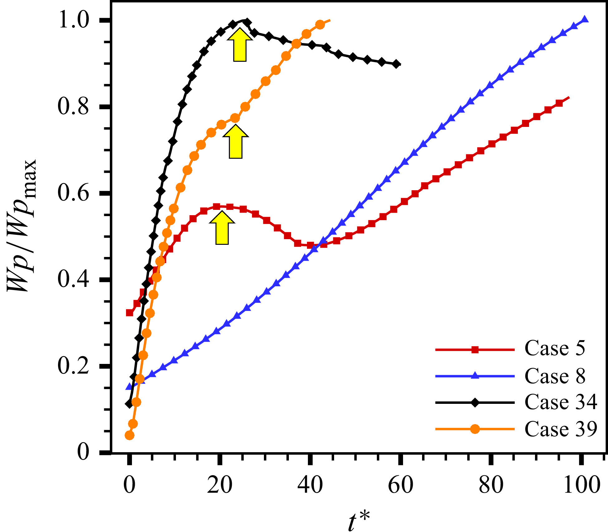
) without sustained LMS compression. However, collision events in case 5 become significant during
 $20 \lt t^* \lt 50$
, coinciding with the LMS–particle interaction period (see figure 14), indicating that collisions are substantially enhanced during the interaction. The time evolution of
 $|\boldsymbol{a}_{\textit{drag}}|_{{avg}}$
(panel b) exhibits a parabolic trend, whereas
 $|\boldsymbol{a}_{\textit{drag}}^*|_{{avg}}$
increases rapidly and cases 1–8 all peak at
 $t\boldsymbol{\cdot }c/r_c =1$
. Meanwhile,
 $|\boldsymbol{a}_{\boldsymbol{\nabla }P_{\!f}}^*|_{{avg}}$
(panel c) decays immediately from
 $t\boldsymbol{\cdot }c_c/r_0 = 0$
and subsequently approaches zero. Overall,
 $|\boldsymbol{a}_{\textit{drag}}^*|_{{avg}}$
becomes the dominant force due to its huge magnitude and continuous action on particles, revealing a time-dependent stage among these forces.
In the early stage, the L(R)MS propagates outward, while the expansion wave moves inward, accelerating the fluid, generating a pressure-gradient force and drag force. Subsequently, a collision force arises from the velocity differences among the outer and inner particles. Here, collisions can be identified as occurring mainly in the upwind region as shown in figure 18. After the expansion wave converges at the centre, the pressure-gradient force approximately vanishes (see figure 17,
 $t\boldsymbol{\cdot }c/r_c \approx 2$
) and the drag force decays related to the decreasing gas–particle relative velocity (see figure 20).
Particle contour plots of
 $|\boldsymbol{a}_{col}^*|$
for case 3 (a) and case 5 (b,c).

Particle contour plots of
 $|\boldsymbol{a}_{\textit{drag}}^*|$
at a microsecond scale for case 3.

The drag force is analysed in detail with spatial and temporal distribution, due to its dominant magnitude and rapid variation within a short time, as shown in figure 19. In general,
 $|\boldsymbol{a}_{\textit{drag}}^*|$
initially increases to a peak during the blast stage and subsequently decays, after which it is sustained by a relatively stable driving from the incoming flow. In detail, the high-
 $|\boldsymbol{a}_{\textit{drag}}^*|$
region propagates inward for
 $t^* \lt 0.316$
, corresponding to the inward expansion wave head. Between
 $0.316 \lt t^* \lt 0.421$
, a transition occurs as the expansion wave converges at the centre (
 $t \boldsymbol{\cdot }c_c/r_0 = 1$
or
 $t^* \approx 0.316$
). Subsequently, the high-drag region shifts to outward diffusion while a low-
 $|\boldsymbol{a}_{\textit{drag}}^*|$
core emerges, attributed to the decreasing gas–particle relative velocity (see figure 20). This decay effect reaches its minimum value around
 $t^* = 1.16$
, and then the streamwise flow becomes the dominant contributor to particle acceleration. In addition, the head of the expansion wave propagates along characteristic lines governed by (5.8):
 \begin{equation} \frac {{\rm d}r}{{\rm d}t} = u - c .\end{equation}
Since the unaccelerated region remains nearly quiescent, the wave head (leading edge) advances inward at
 ${\rm d}r/{\rm d}t \approx -c_c$
, where
 $c_c = \sqrt {\gamma R T_c}$
. The region passed by the expansion head is continuously accelerated, explaining the inward propagation of the high-drag region in figure 19. Furthermore, the radius-time relation for the inward-propagating expansion wave can be expressed as
 $r_{{exp}} = r_c - c_c t$
(here
 $r_c = d_c/2$
). The wave head reaches the centre at
 $t_0^{r_c} = {d_c}/{2c_c}$
(i.e.
 $t_0^{r_c} c_c/r_c = 1$
), which agrees well with figure 17 (
 $|\boldsymbol{a}_{\textit{drag}}^*|_{avg}$
peaking at
 $t\boldsymbol{\cdot }c/r_c = 1$
). Moreover, the transformation
 $t^* = {t c_c}/{r_0} \boldsymbol{\cdot } {c_e M_{\textit{in}}}/{2c_c}$
yields a theoretical convergence time
 $t^* = 0.327$
, approximately close to the observed value
 $t^* = 0.316$
in figure 19.
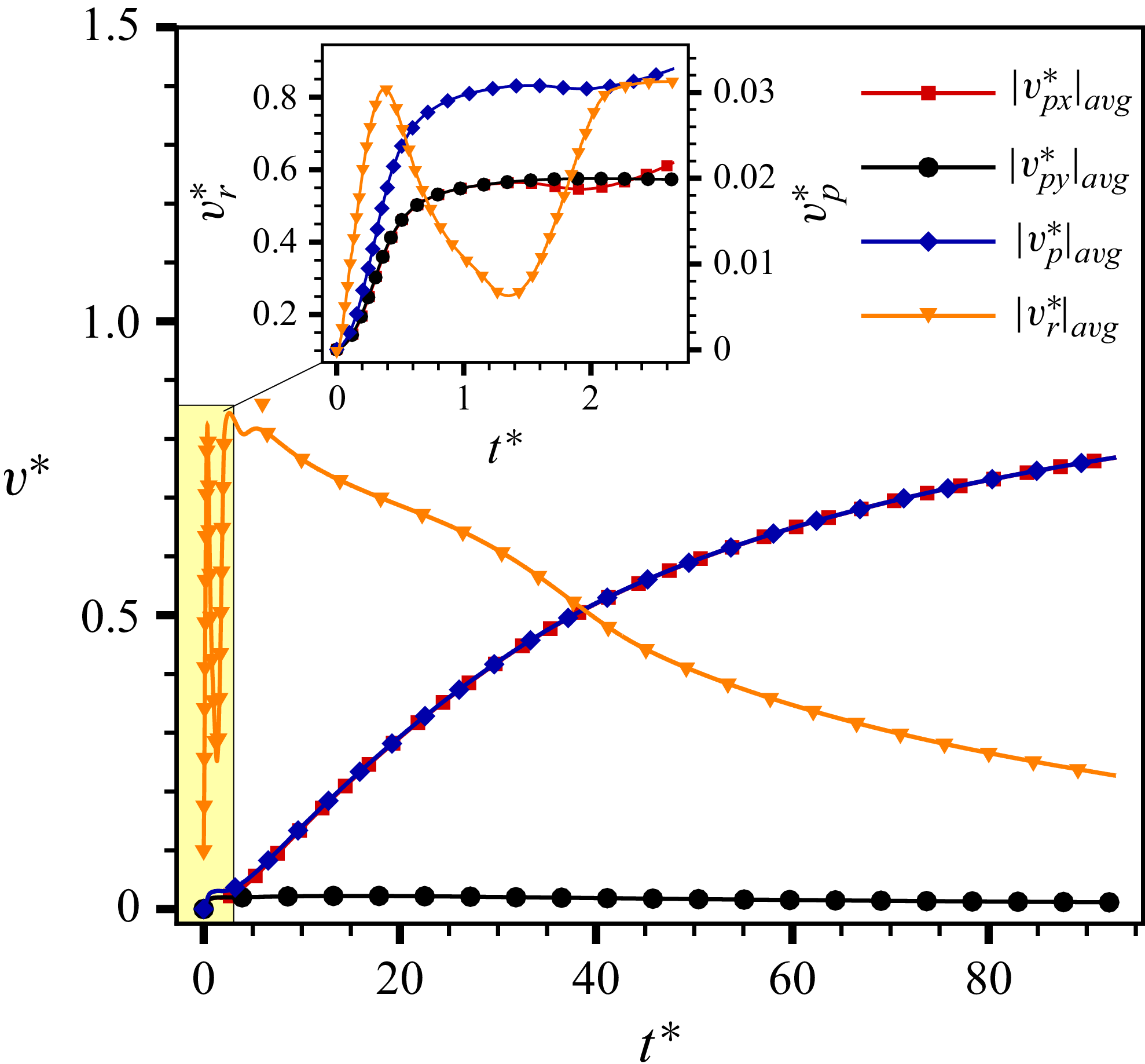
The curves of average
 $|v_{\!px}^*|$
,
 $|v_{\!py}^*|$
,
 $|v_{\!p}^*|$
and
 $|v_{r}^*|$
as a function of
 $t^*$
.

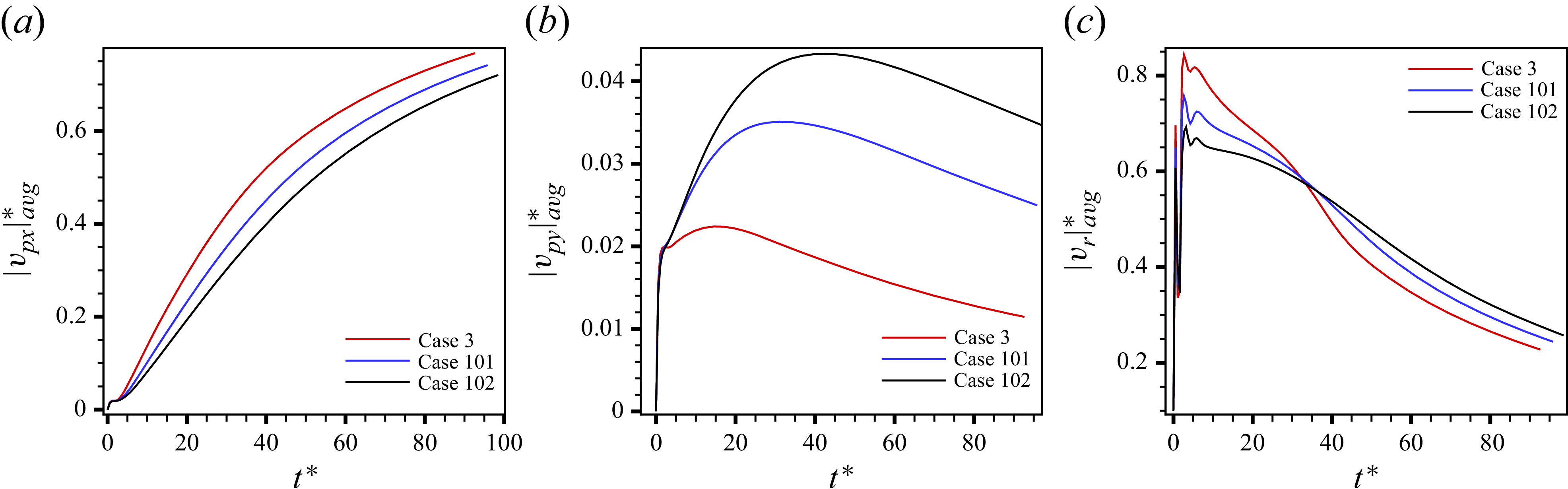
Since particle velocity evolution directly reflects the forces, we preliminarily examine the time-dependent behaviour of average velocities. We define
 $\eta _5^i = |v_{\!px,i}^*|$
,
 $\eta _6^i = |v_{\!py,i}^*|$
,
 $\eta _7^i = |v_{\!p,i}^*|$
and
 $\eta _8^i = |v_{r,i}^*| = |\boldsymbol{\bar u}_{\!f}^* - \boldsymbol{v}_{\!p,i}^*|$
(gas–particle relative velocity), with their statistical averages shown in figure 20. During the early stage (
 $t^* \lt 1.16$
), both the gas and particles are accelerated by the expansion wave. The relative velocity
 $|\boldsymbol{v}_r^*|_{{avg}}$
significantly exceeds
 $|v_p^*|_{{avg}}$
due to particle lag and exhibits fluctuations correlated with drag force variations. For
 $t^* \gt 1.16$
, the streamwise flow increases
 $|\boldsymbol{v}_r^*|_{{avg}}$
, which then gradually decreases as the particles accelerate. Eventually, particle motion becomes streamwise-dominated with
 $|v_p^*|_{{avg}} \approx |v_{\!px}^*|_{{avg}}$
.
5.4.2. Dispersion and dynamics
Particle dispersion and dynamics jointly characterise both the range of particle dispersion and their transport behaviour. Therefore, we focus on investigating the influence of dimensionless parameters on the spanwise dispersion range of the particle cloud, as well as establishing scaling laws for particle dynamics in this section.
Evolution of
 $Y_{{\min}}^*$
,
 $Y_{{\max}}^*$
and
 $U_m^*$
versus
 $t^*$
for particles diffusion based on cases1-8. Panels (a–c) show how varying
 $\varPi _p$
,
 $M_{\textit{in}}$
and
 ${\textit{St}}$
affects the spanwise dispersion of the particle cloud, respectively. Panel (d) shows the evolution of the cloud average velocity
 $U_m^*$
.

The Y-directional dispersal (impact range) of the particle cloud is quantified by
 $Y_{{\min}}$
and
 $Y_{{\max}}$
. The kinetic intensity of the cloud is measured by
 $U_m^*$
. The evolution of the dimensionless quantities
 $Y_{{\min}}^*$
,
 $Y_{{\max}}^*$
and
 $U_m^*$
with respect to
 $t^*$
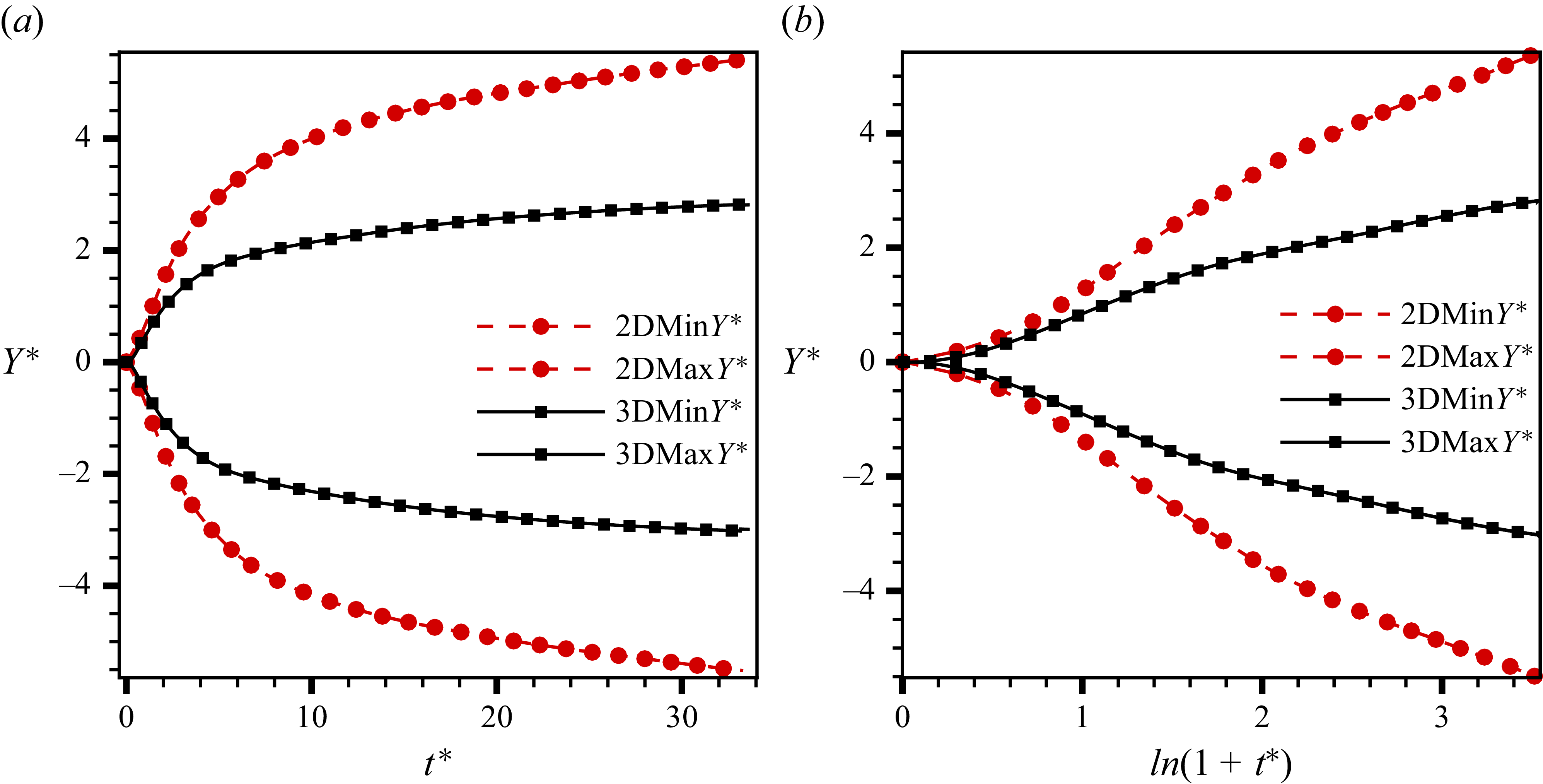
are illustrated in figure 21(a–c), which suggest that stronger blasts give shorter particle response times and lower inflow velocities lead to greater Y-directional dispersion of the particle cloud. It can be explained that high
 $\varPi _p$
increases the initial velocity of the particles while low
 ${\textit{St}}$
enhances the capability of the following gas, and low
 $M_{\textit{in}}$
extends the evolution of the cloud. As shown in panel (d), the particle cloud’s kinetic intensity
 $U_m^*$
exhibits an initial linear increase across all cases. It is modulated by three parameters, while the relaxation behaviour beyond
 $t^* \gt 1$
is primarily governed by
 $M_{\textit{in}}$
and
 ${\textit{St}}$
. To capture broader trends of spanwise dispersion and motion, all cases are synthesised in figure 22. The evolution of
 $Y_{{\min}}^*$
and
 $Y_{{\max}}^*$
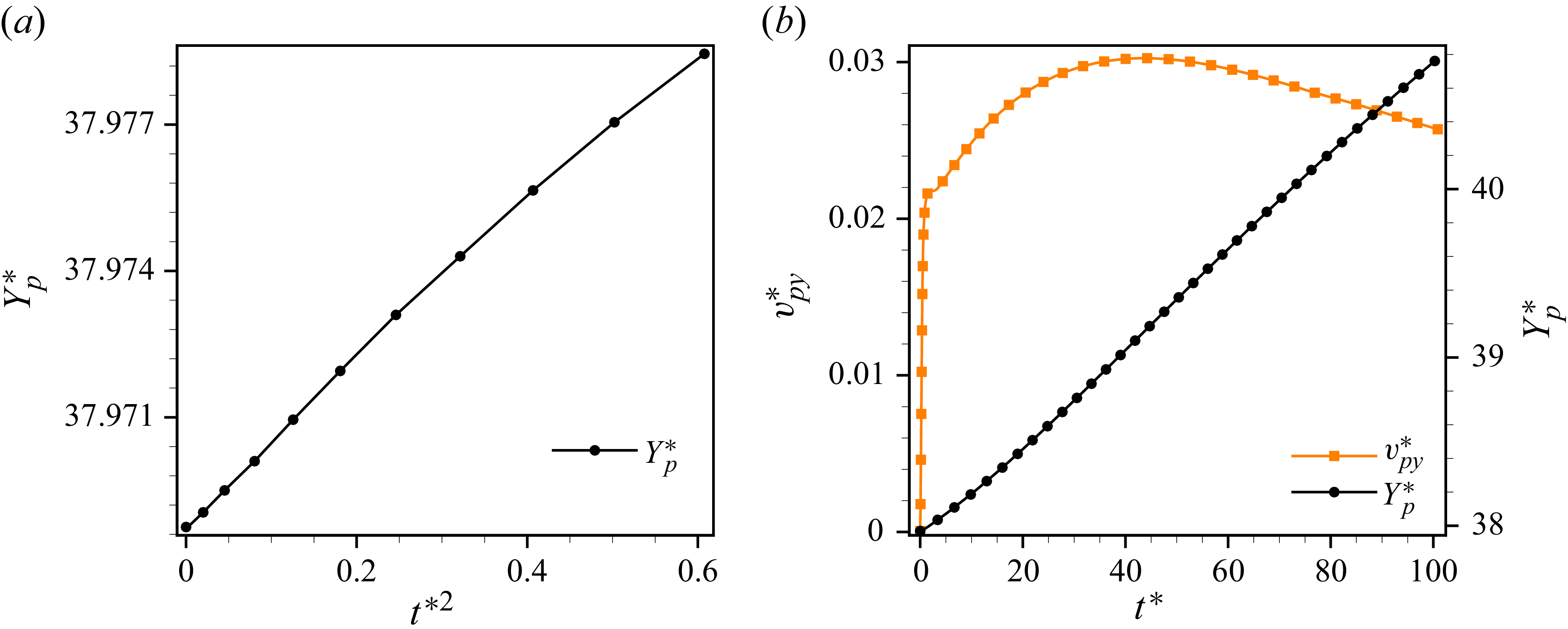
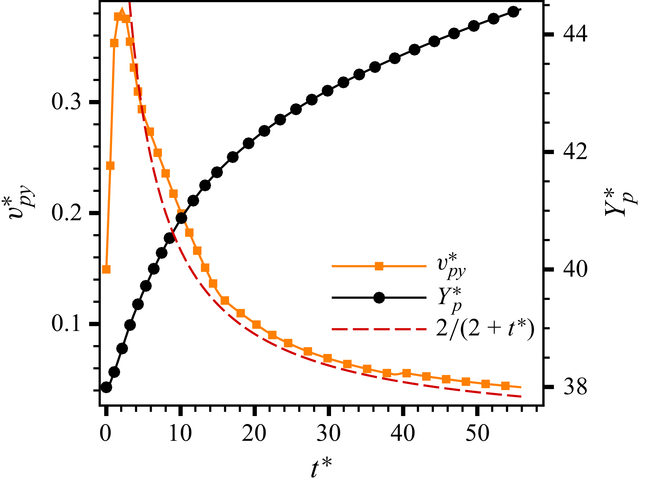
exhibits distinct patterns – linear, quasi-linear and nonlinear – exhibiting a multi-modal character. Specifically, cases 33 and 34 constitute the lower and upper limiting cases of the dispersion range, while other cases fall into a transitional state between them. To interpret this transitional behaviour, we aim to simplify and derive a scaling law for vertical dispersion based on the particle dynamics equation, enabling us to describe the factors of the transition, as detailed in the following derivation.
Evolution of
 $Y_{{\min}}^*$
and
 $Y_{{\max}}^*$
versus
 $t^*$
for particles dispersion based on all cases. The portion of the curve highlighted by yellow boxes exhibits a more linear trend.

According to the particle dynamic equation (2.2), we focus on the leading particle reaching the furthest Y-directional displacement. Based on the Magnus and collision acceleration in figure 34(a) and the integration with time in figure 34(c) (see Appendix A), the collision and pressure-gradient
 $ {\partial P_{\!f}}/{\partial y}$
terms in the Y direction for the leading particle can be neglected, as expressed in (5.9):
 \begin{align} \frac {\text{d} v_{\!py}}{\text{d} t} &= \frac {\kappa _p}{\rho _pV_p} (u_{\!fy} - v_{\!py}), \end{align}
where
 \begin{align} \frac {\kappa _p}{\rho _pV_p}&=\frac {3C_d}{4}\frac {\rho _{\!f}}{\rho _p}\frac {1}{d_p}\boldsymbol{\cdot }|u_{\!fy}-v_{\!py}|, \end{align}
 \begin{align} \frac {\text{d} v_{\!py}}{\text{d} t} &= \frac {\xi }{d_p} \boldsymbol{\cdot }(u_{\!fy} - v_{\!py})^2. \end{align}
It should be noted that the following derivation pertains exclusively to the leading particle located at
 $Y_{{\max}}$
, and the resulting scaling laws are applicable only to this leading particle. Universal variable names (e.g.,
 $Y_p, v_{\!py}$
) are used throughout to avoid subscript redundancy. Considering distinct time scales, the dynamics is divided into a blast-dominated stage and a flow-impingement stage. Here,
 $\xi = {3C_d}/{4} ({\rho _{\!f}}/{\rho _p}) \boldsymbol{\cdot }\text{sgn}(u_{\!fy} - v_{\!py})$
can be positive or negative. In the current analysis, the time dependence of
 $\xi$
is neglected.
The characteristic time scale
 $\eta$
based on the expansion wave propagation (see figure 17
b–c) and its dimensionless form are defined as
 \begin{equation} \eta = \frac {d_c}{c_c} ;\quad \eta ^* = M_{\textit{in}}\sqrt {\frac {T_e}{T_c}} ,\end{equation}
where
 $c_c = \sqrt {\gamma\! \textit{RT}_c}$
is the sound speed within the cloud. For the blast-dominated stage (
 $t \lt \eta$
), the gas velocity at the cloud boundary is determined by the centred simple wave solution. The expansion wave is governed by two families of characteristics
 $C_\pm : {\rm d}x/{\rm d}t = u \pm c$
. Along
 $C_+$
characteristics, the Riemann invariant is conserved as
 \begin{equation} J_+ = \left (u + \frac {2c}{\gamma -1}\right )_{{\textit{point}\,1}} = \left (\frac {2c_c}{\gamma -1}\right )_{{\textit{point}\,0}}\!, \end{equation}
yielding
 $c = c_c - {\gamma -1}/{2}(u)$
. For the centred simple wave, we have
 $\chi = {x}/{t} = u - c$
. Combining the two relations yields
 $u = {2}/({\gamma +1})(\chi + c_c)$
. At the cloud boundary (
 $x=0,\chi = 0$
), the gas velocity can be expressed as
 \begin{equation} U_0 = \frac {2c_c}{\gamma +1} = \frac {2\sqrt {\gamma\! \textit{RT}_c}}{\gamma +1} .\end{equation}
With
 $u_{\!fy} = U_0$
, the integration of (5.11) can be expressed as
 \begin{align} v_{\!py}(t) &= U_0 \boldsymbol{\cdot }\left (1-\frac {1}{1 + \frac {t}{\tau _0}}\right )\!, \end{align}
 \begin{align} Y_p(t) &= U_0 t - \frac {d_p}{\xi }\ln \left (1 + \frac {t}{\tau _0}\right )\!, \end{align}
where a characteristic response time emerges naturally as
 $\tau _0 = {d_p}/{\xi U_0}$
. At
 $t = \eta$
, the particle velocity and displacement are
 \begin{align} v_{\!p\eta } &= U_0 \boldsymbol{\cdot }\left (1-\frac {1}{1 + \frac {\eta }{\tau _0}}\right )\! ,\end{align}
 \begin{align} Y_{\!p\eta } &= U_0 \eta - \frac {d_p}{\xi }\ln \left (1 + \frac {\eta }{\tau _0}\right )\!. \end{align}
In dimensionless form,
 \begin{align} v_{\!p\eta }^* &= \frac {U_0}{u_{\!f\infty }} \boldsymbol{\cdot }\left (1-\frac {1}{1 + \dfrac {\eta }{\tau _0}}\right )\! ,\end{align}
 \begin{align} Y_{\!p\eta }^* &= \frac {U_0\eta }{d_c} - \frac {d_p}{\xi d_c}\ln \left (1 + \frac {\eta }{\tau _0}\right )\!, \end{align}
where
 $ {U_0\eta }/{d_c}= {2}/{\gamma +1}$
and the key dimensionless ratio governing the particle response is
 \begin{equation} \frac {\eta }{\tau _0} = \frac {\xi U_0 d_c}{c_cd_p} .\end{equation}
The scaling behaviour for
 $t \lt \eta$
is determined by the ratio
 $({\eta }/{\tau _0})$
.
When
 $ {\eta }/{\tau _0} \ll 1$
(large/heavy particles or weak blasts), the Taylor expansion of (5.15) and (5.16) gives
 \begin{equation} Y_{\!p}^* \propto t^{*2} ,\qquad v_{\!py}^* \propto t^* .\end{equation}
The streamline diagram for case 34 at
 $t^*=2.63$
(particles plotted in purple).

When
 $ {\eta }/{\tau _0} \gg 1$
(without any lag effects, which is easy to understand but not in our interests), the particle quickly reaches the gas velocity, giving
 \begin{equation} Y_{\!p}^* \propto \frac {U_0}{u_{\!f\infty }} t^* ,\qquad v_{\!py}^* \xrightarrow {} \frac {U_0}{u_{\!f\infty }} .\end{equation}
In addition,
 $\xi = {3C_d}/{4} ({\rho _{\!f}}/{\rho _p})$
, while the expanded density
 $\rho _{\!f}$
satisfies the isentropic relation
 \begin{equation} \frac {\rho _{\!f}}{\rho _c} = \left (\frac {c}{c_c}\right )^{({2}/{\gamma -1})} = \left (\frac {2}{\gamma +1}\right )^{({2}/{\gamma -1})} \equiv \phi. \end{equation}
The initial cloud density is
 $\rho _c = \rho _e\varPi _p ({T_e}/{T_c})$
. Thus, the gas density at the cloud boundary after expansion is
 \begin{equation} \rho _{\!f} = \phi \boldsymbol{\cdot }\rho _e \boldsymbol{\cdot }\varPi _p \boldsymbol{\cdot }\frac {T_e}{T_c}, \end{equation}
and
 $\xi$
can be written as
 \begin{equation} \xi = \frac {3C_d}{4}\frac {\rho _{\!f}}{\rho _p} = \frac {3\phi C_d \varPi _p}{4} \frac {T_e}{T_c}\frac {\rho _e}{\rho _p} .\end{equation}
For
 $t \gt \eta$
, due to expansion effects and the LMS acting as a bow shock,
 $u_{\!fy} \ne 0$
. As shown in figure 23, the inflow passes through the curved leading main shock (i.e the LMS). Due to the curvature of the LMS, the post-shock flow is deflected from the original X direction, producing a Y-directional velocity component, i.e.
 \begin{equation} U_\infty \propto V_{\!post} \boldsymbol{\cdot }\sin \theta _{\textit{LMS}}, \end{equation}
where
 $V_{\!post}$
is the post-shock gas velocity magnitude and
 $\theta _{\textit{LMS}}$
is the local flow deflection angle (
 $\theta _{\textit{LMS}} = 0$
when the LMS passes through the particle cloud). In the long term,
 $ U_\infty$
varies slowly with time, the integration of (5.11) for
 $t \gt \eta$
is
 \begin{align} v_{\!py}(t) &= U_\infty - \frac {1}{\dfrac {1}{ U_\infty -v_{\!p\eta }} + \dfrac {\xi }{d_p}(t-\eta )}, \end{align}
 \begin{align} Y_{\!p}(t) &= Y_{\!p\eta } + U_\infty (t-\eta ) - \frac {d_p}{\xi } \ln \left | 1+\xi \frac {(U_\infty - v_{\!p\eta })}{d_p}(t-\eta ) \right |. \end{align}
In dimensionless form,
 \begin{equation} Y_{\!p}^*= Y_{\!p\eta }^* + \frac {U_\infty }{u_{\!f\infty }}(t^*-\eta ^*) + \frac {d_p}{\xi d_c}\ln \left | 1+\frac {\xi d_c}{d_p}\frac { (U_\infty - v_{\!p\eta })}{u_{\!f\infty }}(t^*-\eta ^*) \right | .\end{equation}
The long-term behaviour is determined by the velocity ratio
 $\mathcal{R} = {v_{\!p\eta }}/{U_\infty }$
.
When
 $\mathcal{R} \ll 1$
(i.e.
 $v_{\!p\eta } \ll U_\infty$
, large/heavy particles or weak blast relative to the inflow), the particle continues to accelerate, which can be simplified as
 \begin{equation} Y_{\!p}^*\propto \frac {U_\infty }{u_{\!f\infty }}t^* ,\qquad v_{\!py}^* \to \frac {U_\infty }{u_{\!f\infty }} .\end{equation}
When
 $\mathcal{R} \gg 1$
(i.e.
 $v_{\!p\eta } \gg U_\infty$
, corresponding to small/light particles or a strong blast relative to the inflow), the particle decelerates, which can be simplified as
 \begin{equation} Y_{\!p}^*\propto \ln \left |1+kt^*\right | ,\qquad v_{\!p}^*\propto \frac {1}{\dfrac {1}{k}+t^*} ,\end{equation}
where
 $k = {\xi d_c}/{d_p} ({(v_{\!p\eta } - U_\infty )}/{u_{\!f\infty }})$
. When
 $\mathcal{R} \sim 1$
, the behaviour is intermediate between linear and logarithmic. This transition is an inherent property of the solution (5.29). The spectrum of behaviours observed in figure 22 reflects the transition trends.
Overall, the particle motion is simplified into two stages governed by gas velocities
 $U_0$
(for
 $t \lt \eta$
) and
 $U_\infty$
(for
 $t \gt \eta$
). Here
 $U_0 = 2c_c/(\gamma +1)$
follows from the centred simple wave solution for the leading particle, while
 $U_\infty \propto M_{\textit{in}} c_e \sin \theta _{\textit{LMS}}$
arises from flow deflection across the curved LMS. The particle velocity and displacement are obtained by integrating (5.11), yielding (5.15) and (5.16) for
 $t \lt \eta$
and (5.28) and (5.29) for
 $t \gt \eta$
. Based on the solution structure, the scaling laws emerge as special cases depending on
 $ {\eta }/{\tau _0}$
and
 $ {v_{\!p\eta }}/{U_\infty }$
. Validation for the scaling laws in these special cases is provided in figures 35 and 36 (see Appendix A).
5.4.3. Morphologies of dispersion
As particles disperse over time, it is noted that their distribution forms typical morphologies. Subsequently, this section focuses on exploring the quasi-steady morphology of the particle cloud, the underlying physical mechanisms and the effects of the governing dimensionless parameters.
The morphology of cloud and wave structures is essential to explore. As discussed in § 5.3, the LMS impinged the particle cloud, leading to spanwise dispersion in figure 15. As can be seen for case 33 in figure 16(b), the cloud is interacting with the DCS vortex but is farther from the LMS. Moreover, as previously shown in figure 14 (see § 5.3), the morphologies of both case 3 and case 4 are similar to circular or elliptical. While the shape is a crescent in case 5 due to sustained compaction between the LMS and particles. To quantitatively categorize these morphologies, we introduce ‘compaction index’ and ‘density uniformity’. The morphology is characterised by two indices. Particle coordinates are first normalised by the vertical extent
 $L_y = y_{{\max}} {-} y_{{\min}}$
, giving dimensionless coordinates
 $\tilde {x} = (x {-} x_{{\min}})/L_y$
and
 $\tilde {y} = (y {-} y_{{\min}})/L_y$
. The compactness index (CI) measures the normalised enclosed area of the particle cloud and is defined as
 \begin{equation} \text{CI} = \left ( \int _0^1 \left [ \tilde {x}_{{\max}}(\tilde {y}) - \tilde {x}_{{\min}}(\tilde {y}) \right ] d\tilde {y} \right )^2, \end{equation}
where
 $\tilde {x}_{{\max}}(\tilde {y})$
and
 $\tilde {x}_{{\min}}(\tilde {y})$
denote the rightmost and leftmost normalised particle positions at height
 $\tilde {y}$
. A larger CI indicates a more dispersed particle cloud, while a smaller CI corresponds to a more compact cloud. The density uniformity (DU) quantifies how evenly particles are spaced. For each particle
 $i$
, the local spacing
 $\tilde {d}_i$
is the nearest-neighbour distance in normalised coordinates:
 \begin{equation} \tilde {d}_i = \min _{j \neq i} \| \tilde {\boldsymbol{x}}_i - \tilde {\boldsymbol{x}}_j \|. \end{equation}
The DU is defined as
 \begin{equation} \text{DU} = \frac {\bar {\tilde {d}}^2}{\sigma _{\tilde {d}}^2}, \end{equation}
where
 $\bar {\tilde {d}}$
and
 $\sigma _{\tilde {d}}$
are the mean and standard deviation of
 $\{\tilde {d}_i\}$
. A larger DU indicates uniform particle spacing, while a smaller DU suggests clustering or the presence of density concentrations. Based on (5.33) and (5.35), the CI and DU values for all cases are computed and normalised, as shown in figure 24.
Scatter plot of the CI versus DU for all simulated cases. The parameter space is divided into four morphology categories: uniform (high CI, high DU), eroded (low CI, high DU), compressed (low CI, low DU) and jetting (high CI, low DU). Case numbers are labelled within or nearby each marker.

According to the definitions, the CI represents the ratio of the streamwise width to the spanwise height of the particle cloud (equivalently, the ratio of the envelope area to the area of a square with side length
 $L_y$
), while the DU characterises the uniformity of particle spacing. Based on the CI and DU, the morphologies can be classified into four categories. We select representative case results as the corresponding morphology in figure 24: case 5 (compressed), case 8 (uniform), case 34 (eroded) and case 39 (jetting). A notable observation is that, except for the uniform morphology, all other categories exhibit significant changes in streamwise thickness. This suggests that the morphology differences are closely related to the deformation processes experienced by the particle cloud.
Temporal evolution of the streamwise and normalised particle cloud thickness
 $W_p /W_{\!p{\max}}$
for representative cases: case 5 (compressed), case 8 (uniform), case 34 (eroded) and case 39 (jetting).

Therefore, the temporal evolution of
 $\tilde {W_p}=W_p /W_{\!p{\max}}$
can be investigated to explore the potential mechanism, as shown in figure 25. The results reveal that case 8 (uniform) exhibits a nearly steady increase in
 $\tilde {W_p}$
. In contrast, the other three cases show distinct transitions at specific times, marked by yellow arrows in the figure. For case 5 (compressed) and case 34 (eroded), the initially increasing
 $\tilde {W_p}$
reaches a maximum and subsequently decreases. Conversely, for case 39 (jetting), the growth rate of
 $\tilde {W_p}$
accelerates after the marked position. As discussed in § 5.3, multiple wave structures including LMS, RMS, DSCL and SSL, SSR are present in the flow field. Given the observed correlation between morphology categories and thickness evolution, we further examine how specific wave–particle interactions lead to the distinct deformation characteristics of each category. Figure 26 presents the temporal evolution of wave positions and particle cloud boundaries along the streamwise centreline for these representative cases.
Temporal evolution of wave positions and particle cloud boundaries along the streamwise centreline for representative cases: (a) case 5 (compressed), (b) case 8 (uniform), (c) case 34 (eroded) and (d) case 39 (jetting). Solid lines denote wave structures (LMS, RMS, DSCL, SSL, SSR) and dashed lines indicate the particle cloud front (
 $x_{{\min}}$
) and rear (
 $x_{{\max}}$
) boundaries.

As shown in figure 26(a), the LMS continuously interacts with the particle cloud during
 $t^* \approx 10$
–
 $50$
. The particle front position (
 $X_{{\min}}^*$
) decreases while the rear boundary (
 $X_{{\max}}^*$
) remains relatively stationary, indicating strong streamwise compaction driven by the LMS. This corresponds to the thickness reduction observed in figure 25. Passage of the LMS creates discontinuous gas states across the shock front, causing particles to accumulate non-uniformly, which explains the low DU and low CI.
In figure 26(b) the particle front continually interacts with the SSL only during the later stage of the entire process, when the SSL strength has already weakened considerably (see figure 13). Consequently, the particle cloud thickness expands steadily over time without abrupt changes. This explains the formation of the uniform morphology, characterised by high DU and high CI values.
In figure 26(c) the DSCL remains in close proximity to the particle cloud boundary throughout almost the entire process. This persistent DCS–particle interaction induces erosion at the cloud periphery, progressively stripping away particles from the outer layers while the core region maintains its structure. The gradual decrease in thickness observed in figure 25 reflects this erosion process. Unlike the compressed case where the LMS causes abrupt compression with non-uniform accumulation, the DCS-induced erosion is a progressive process that reduces the envelope area (low CI) while preserving relatively uniform spacing in the remaining core (high DU).
Figure 26(d) shows that the key event occurring near the particle boundary during
 $t^* \approx 20$
–
 $25$
is the convergence and subsequent outward propagation of the SSL and SSR. This time interval corresponds to the rapid increase in
 $\tilde {W_p}$
observed in figure 25. As discussed in § 5.2.2, the convergence of the SecS leads to a sharp increase in shock strength and post-shock velocity (see figure 13) (Ling & Balachandar Reference Ling and Balachandar2018a
), forming localised high-velocity channels. The channel entrains and transports particles downstream, forming jet-like structures that extend the particle cloud boundary significantly. The formation of jets increases the envelope area (high CI) while creating significant density variations between jet and non-jet regions (low DU).
The above analysis demonstrates that the proposed morphology classification reflects distinct physical mechanisms, and the correlation between wave positions and particle cloud thickness evolution provides quantitative evidence for this interpretation. Specifically, (i) the compressed morphology is dominated by LMS-induced compaction, where discontinuous gas states cause non-uniform accumulation; (ii) the uniform morphology arises from weak wave–particle interactions that preserve the cloud structure; (iii) the eroded morphology results from DCS-induced peripheral erosion, where counter-rotating vortices strip particles from the leeward region while preserving core uniformity; and (iv) the jetting morphology is driven by SecS-induced high-velocity channels that create jet structures.
Given the high dimensionality of the parameter space, we are primarily concerned with aerodynamic effects and particle responses to these effects. Based on the analysis presented in the preceding sections, the LMS behaviour is closely related to
 $M_{\textit{in}}$
, particle responsiveness scales with
 ${\textit{St}}$
, and SecS strength correlates with
 $\varPi _p$
. Therefore, we focus on these three dimensionless parameters and classify cases to obtain the distribution of different morphologies, i.e. the phase diagram shown in figure 27.
The phase diagram reveals the correlation between the parameters
 $(M_{\textit{in}}, \varPi _p, St)$
and the resulting particle cloud morphology. Consistent with our mechanistic analysis, the compressed morphology dominates in the region of large
 $M_{\textit{in}}$
and relatively large
 ${\textit{St}}$
, where the fast-propagating LMS overtakes and compacts the particle cloud. In contrast, for relatively small
 ${\textit{St}}$
and
 $M_{\textit{in}}$
, the particle cloud remains in close proximity to the DCS and experiences deceleration by the low-velocity region between the counter-rotating vortex pair, resulting in the eroded morphology. When the pressure ratio
 $\varPi _p$
is sufficiently high, the SecS strength increases (see figure 13
a), enhancing the high-velocity channel effect. Particles with small
 ${\textit{St}}$
readily follow the accelerated gas flow, forming particle jets; accordingly, the phase diagram shows that the jetting morphology is associated with the highest
 $\varPi _p$
values. The uniform morphology requires moderate
 ${\textit{St}}$
and
 $M_{\textit{in}}$
to maintain sufficient separation between the particle cloud and the surrounding waves. Even at elevated
 $\varPi _p$
, particle clouds with relatively low responsiveness (large
 ${\textit{St}}$
) remain distant from the converging SecS, and thus, do not develop jet structures within the observation time.
A phase diagram of the particle cloud related to
 $M_{\textit{in}},St$
and
 $\varPi _p$
.

6. Preliminary dimensional effects analysis
In order to investigate the dimensional effects, we focus on comparing the similarities and differences of wave structures and morphology of particle cloud. The 3D simulation is first set up with initial conditions (including boundary, inflow, particle-driven conditions) identical to the 2D case. Considering the high computational cost of the 3D simulations, a preliminary investigation is conducted based on a 3D case with approximately
 $4.5\times 10^6$
grid cells. The number of grids in three directions is set to
 $(N_x,N_y,N_z)=(200,150,150)$
with the enlarged high-pressure regime
 $d_c = 0.6m$
and the 2D case is adjusted accordingly. Figure 28(a) shows the presence of LMS and SecS, along with the DCS vorticity isosurfaces in the wake of the particle cloud, where no detached shock is observed, likely due to the reduced gas–particle relative velocity. Figure 28(b) illustrates the particle cloud morphology and slice of the DCS vorticity contour, consistent with the 2D case. However, due to the expanded domain, the DCS may evolve to erode and compress the particle cloud, resulting in the eroded-type morphology.
A 3D simulation validation based on the initial conditions of two dimensions. Panel (a) illustrates the wave structures including LMS, SecS and DCS in the 3D flow field (only
 $\boldsymbol{\nabla} _x\rho _{\!f}$
is shown). Panel (b) shows the vorticity distribution and particle morphology belonging to the eroded type.

In addition, the proposed scaling laws are not dimension dependent. Thus, the evolution of
 $Y_p^*$
and
 $v_{\!py}^*$
should follow the same trends as derived. As shown in figure 29,
 $Len_y^*$
and
 $Len_z^*$
are symmetric in the absence of gravity, exhibiting a
 $t^{*2}$
trend for
 $t \lt \eta$
, while
 $t \gt \eta$
,
 $v_{\!py}^*$
decays as
 $t^{*-1}$
and
 $Y_p^*$
grows logarithmically. This work aims to directly compare the 2D results with the 3D results. As shown in figure 30(a), both exhibit similar trends, while the particle dispersion ability of a 2D simulation is stronger than that of a 3D simulation. This is primarily attributed to the additional degree of freedom in the 3D energy release, which leads to a reduced proportion of kinetic energy transferred to particles in the Y direction. The effective comparison suggests that they are related and may be proportional in some way. In panel (b) a logarithmic coordinate result also verifies the assumption of two stages because of the segmented linear stage.
Panels (a) and (b) verify the scaling laws in two stages,
 $t\lt \eta$
and
 $t\gt \eta$
, where Y and Z components exhibit symmetry.

A comparative analysis is conducted on the time evolution of
 $Y_{{\max}}^*$
and
 $Y_{{\min}}^*$
in the Y direction between 2D and 3D case. (a) The comparison validates dimensional effects and demonstrates the similarity in particle dispersion behaviour across dimensions. (b) A logarithmic scale is applied to
 $t^*$
to verify the log-type growth law
 $Y_{\!pt}^*\propto \ln |1+kt^*|$
.

The comparison between 2D and 3D simulations reveals both qualitative similarities and quantitative differences. In terms of similarities, both simulations exhibit the same wave structures, including LMS, SecS and DCS. The proposed scaling laws are also dimension independent: it can be observed in both 2D and 3D results that
 $Y_p^* \propto t^{*2}$
for
 $t^* \lt \eta$
and, for logarithmic growth,
 $v_{\!py}^* \sim t^{*-1}$
for
 $t^* \gt \eta$
. This confirms that the theoretical framework developed in § 5.4.2 applies to both 2D and 3D configurations. In terms of differences, several distinctions are observed. First, the DCS in three dimensions exhibits a more complex vortical morphology, as 3D flows permit vortex stretching effects that are inherently absent in two dimensions. Second, the spanwise dispersion range in three dimensions is smaller than in two dimensions at corresponding dimensionless times. Third, the particle cloud morphology differs in three dimensions, exhibiting a particle distribution in the out-of-plane direction, which cannot be captured by 2D simulations.
7. Conclusions
This study investigated the dispersion of particle clouds driven by the coupling of blast waves and supersonic inflow, employing the CMP-PIC method. Through systematic numerical simulations and theoretical analysis across a broad parameter space, we elucidated the wave structures, wave–particle interactions, particle dynamics and dispersion morphologies in this coupled system.
The wave system generated by the blast-inflow coupling exhibits distinct characteristics compared with classical shock-tube or point-source blast configurations. The flow field comprises the LMS/RMS, a DCS, expansion waves and a SecS. Over-expansion creates an implosion environment that generates the SecS at the tail of the expansion wave, which subsequently impinges upon the DCS and triggers a RMI, contributing to deposit vorticity. The main shock velocity–radius relation approximately follows a power-law form
 $r_s^* \propto t^{*k}$
without considering the effects of shock–particle interactions.
The interactions among waves and the particle cloud are closely related to their relative velocities and positions. Increasing
 $M_{\textit{in}}$
causes the LMS to migrate toward and compress the particle cloud. Higher
 $\varPi _p$
intensifies the SecS strength, the time to converge and the high-velocity channels that can entrain particles into jet structures. The Stokes number
 ${\textit{St}}$
characterises particle responsiveness; smaller
 ${\textit{St}}$
enables particles to follow the accelerated gas flow more readily. These interactions – including LMS compression and SecS-driven jetting – ultimately determine the resulting particle cloud morphology.
For particle dynamics, drag force dominates throughout the evolution, reaching its maximum when the expansion wave converges at the centre (
 $tr_c/c_c=1$
) and subsequently sustained by the incoming flow. A two-stage scaling law for spanwise particle dispersion is derived from simplified conditions and equations. During the blast-dominated stage (
 $t \lt \eta$
, where
 $\eta = d_c/c_c$
), the displacement scales as
 $Y_p^* \propto t^{*2}$
. During the subsequent flow-impingement stage (
 $t \gt \eta$
), the scaling transitions from linear growth (
 $Y_p^* \propto t^*$
) to logarithmic growth (
 $Y_p^* \propto \ln |1 + kt^*|$
), depending on the ratio of the blast-induced particle velocity to the inflow-induced gas velocity.
Based on the CI and DU, four distinct particle cloud morphologies are identified: compressed, uniform, eroded and jetting. Each morphology corresponds to a specific dominant mechanism: the compressed morphology results from sustained LMS compression that creates non-uniform particle accumulation; the uniform morphology arises when wave–particle interactions remain weak and the cloud structure is preserved; the eroded morphology is caused by DCS-induced peripheral erosion through counter-rotating vortices that decelerate particles in the leeward region; and the jetting morphology is driven by SecS-induced high-velocity channels that entrain small
 ${\textit{St}}$
particles into jet structures. A phase diagram constructed in the
 $(M_{\textit{in}}, St, \varPi _p)$
parameter space reveals that the compressed morphology dominates at large
 $M_{\textit{in}}$
and
 ${\textit{St}}$
, the eroded morphology occurs at small
 $M_{\textit{in}}$
and
 ${\textit{St}}$
, the jetting morphology is associated with the highest
 $\varPi _p$
values and the uniform morphology requires moderate
 ${\textit{St}}$
and
 $M_{\textit{in}}$
to maintain sufficient separation between the particle cloud and surrounding waves.
Future work may focus on exploring strategies to enhance spanwise dispersion, such as splitting the particle cloud into multiple smaller clouds or employing multiple blast sources. Additionally, extensive 3D simulations could be conducted to develop comprehensive dispersion scaling laws and refine the phase diagram across a broader parameter space. Ultimately, a physical model for the entire system could be established, encompassing the dynamics of various waves, particle cloud evolution and their coupled interactions.
Funding
This work was supported by the National Natural Science Foundation of China (Grants No. 12472262, 12432012, 12388101); the Chinese Academy of Sciences Project for Young Scientists in Basic Research (Grant No. YSBR-132); the Chinese Academy of Sciences (Grants No. XDB1100000, XDB0620203); and the Young Elite Scientists Sponsorship Program of the Beijing High Innovation Plan (Grants No. 20251070).
Declaration of interests
The authors report no conflict of interest.
Author contributions
K. Chen: code modification, numerical simulations, data processing, theory analysis, writing – original draft. B. Meng: supervision, writing – review & editing, methodology, original code, scaling laws, mechanism of particle & wave motion, funding acquisition. B. Tian: methodology, original code, supervision, review, funding acquisition.
Data availability statement
The data that support the findings of this study are available from the corresponding author upon reasonable request.
Appendix A. Supplementary content
This appendix presents supplementary content not covered in detail.
Here we support the method to discretise the nozzling term
 $P_{\!f}\boldsymbol{\nabla }\alpha _p$
as follows. Consider a one-dimensional equation derived from (2.3) as an example:
 \begin{equation} \frac {\partial \boldsymbol{U}'}{\partial t} +\frac {\partial \boldsymbol{F}'}{\partial x} =\boldsymbol{D_p}'. \end{equation}
By discretising (A1) in time and space direction, we obtain
 \begin{align}&\qquad\qquad \frac {\partial \boldsymbol{U}'}{\partial t} = -\frac {\hat {\boldsymbol{F}}^{\prime}_{i+{1}/{2}} - \hat {\boldsymbol{F}}^{\prime}_{i-{1}/{2}}}{\Delta x} + P_{\!f} \frac {\hat {\alpha }^{\prime}_{f,i+ {1}/{2}} - \hat {\alpha }^{\prime}_{f,i- {1}/{2}}}{\Delta x} \begin{bmatrix} 0 & 1 & \bar {v}_{\!px} \end{bmatrix}^T \!, \end{align}
 \begin{align}& S_L = \min (u_{\textit{fxL}} - c_L, u_{\textit{fxR}} - c_R, 0), \qquad S_R = \max (u_{\textit{fxL}} + c_L, u_{\textit{fxR}} + c_R, 0) , \end{align}
 \begin{align}&\qquad\qquad\qquad S_* = \frac { p_R - p_L + \rho _L u_L (S_L - u_L) - \rho _R u_R (S_R - u_R) }{ \rho _L (S_L - u_L) - \rho _R (S_R - u_R) } ,\end{align}
 \begin{align}& \alpha _{f,i+ {1}/{2}} = \begin{cases} \dfrac {S_R \alpha _{\textit{fL}} - S_L \alpha _{\textit{fR}}}{S_R - S_L} & \text{for HLL-type solver}, \\[8pt] \left [ \dfrac {1 + \operatorname {sign}(S_*)}{2} \alpha _{\textit{fL}} + \dfrac {1 - \operatorname {sign}(S_*)}{2} \alpha _{\textit{fR}} \right ]_{i+ {1}/{2}} & \text{for HLLC-type solver}. \end{cases} \end{align}
The discrete algorithms for nozzling terms are given, where the subscript L and R represent the left and right variables. The wave estimations of the
 $S_L/S_R$
are expressed in (A3) and the speed of the contact
 $S_*$
is given in (A4). Ultimately, the discrete forms of the nozzling term to prevent numerical oscillations for a HLL-type solver and HLLC-type solver are expressed in (A5).
Validation of numerical results against experimental data (Rogue et al. 1998) for shock–particle curtain interactions. (a) Diagram of the Rogue test and the probe position. (b) Pressure history tracked by probe 1 and probe 2 for computation and the experiment.

Relative error curves for grid-independence verification. Panels (a–c) correspond to figure 4, with errors calculated relative to the finest mesh M5.

Schlieren image of the DCS with
 $u_{\textit{fx}}$
contour lines.

Temporal evolution of the leading particle dynamics in the spanwise direction: (a) pressure-gradient acceleration
 $a_{\boldsymbol{\nabla }P_{\!fy}}^*$
, (b) collision-induced acceleration
 $a_{{col},y}^*$
, (c) velocity contribution from pressure gradient
 $v_{\!p\boldsymbol{\nabla }P_{\!fy}}^* = \int a_{\boldsymbol{\nabla }P_{\!fy}}^* \, \mathrm{d}t^*$
, and (d) spanwise velocity
 $v_{\!py}^*$
.

(a) Using case 8 as an example, the
 $Y$
position of the furthest particle for
 $t \lt \eta$
shows a linear trend with
 $t^{*2}$
, indicating
 $Y_{\!p}^* \propto {t^*}^2$
; (b)
 $Y_{\!p}^*\propto t^*$
grows near-linearly and
 $v_{\!py}^*\xrightarrow {} {U_\infty }/{u_{\!f\infty }}$
slowly varies after
 $t^* \gt \eta ^*$
.

Case 34:
 $Y_p^*$
follows a logarithmic trend and
 $v_{\!py}^*\propto ({1}/{ {1}/{k}+t^*})$
.

A.1. Dimensionless numbers
Four fundamental units (
 $\rho _e, u_{\!f\infty },d_c,T_e$
) are selected as basic variables for dimensional analysis, deriving 18 mathematically independent dimensionless numbers (A6) by Buckingham theory, and here we apply the equation of state for an ideal gas,
 $P=\rho RT$
, and an equivalent transformation to simplify the redundant parameters:
 \begin{equation} \begin{aligned} \pi _1 &= \frac {P_e}{\rho _e u_{\!f\infty }^2}, \quad \pi _2 = \frac {P_c}{\rho _e u_{\!f\infty }^2}, \quad \pi _3 = \frac {T_c}{T_e}, \quad \pi _4 = \frac {\rho _eu_{\!f\infty }d_c}{{\mu} _{\!f}}, \quad \pi _5 = \frac {\rho _c}{\rho _e}, \quad \pi _6 = \frac {\textit{RT}_e}{u_{\!f\infty }^2},\\ \pi _7 &= \frac {d_p}{d_c}, \quad \pi _8 = \frac {\rho _p}{\rho _e}, \quad \pi _9 = \frac {T_p}{T_e}, \quad \pi _{10}= \frac {t \boldsymbol{\cdot }u_{\!f\infty }}{d_c}, \quad \pi _{11} = \frac {Y_{{\max}}}{d_c}, \quad \pi _{12} = \frac {Y_{{\min}}}{d_c}, \\ \pi _{13} &= \frac {X_p}{d_c}, \quad {\pi _{14}=\frac {|\boldsymbol{v}_r|}{u_{\!f\infty }}}, \quad \pi _{15} = \frac {\omega _z d_c}{u_{\!f\infty }}, \quad \pi _{16} = \frac {X_w}{d_c}, \quad \pi _{17}=\gamma, \quad \pi _{18}=\alpha_p.\end{aligned} \end{equation}
For an ideal gas, since
 $ P_e = \rho _e R T_e$
, the parameters
 $\pi _1$
and
 $\pi _6$
are equivalent, and
 $\pi _5$
is redundant since it can be derived from
 $\pi _2$
,
 $\pi _3$
and the equation of state. Therefore, both
 $\pi _1$
and
 $\pi _5$
are removed. The inflow Mach number is defined as
 \begin{align} M_{\textit{in}} = \frac {u_{\!f\infty }}{\sqrt {\gamma\! \textit{RT}_e}} = \frac {1}{\sqrt {\gamma \pi _6}} , \end{align}
where
 $\gamma$
is constant. Hence,
 $M_{\textit{in}}$
can replace
 $\pi _6$
as an independent dimensionless parameter.
The Reynolds number for the gas phase is expressed as
 \begin{align} {\textit{Re}}_{g} = \frac {\rho _e u_{\!f\infty } d_c}{{\mu} _{\!f}} = \frac {1}{\pi _5}. \end{align}
Furthermore, the particle Reynolds number
 ${\textit{Re}}_{\!p}$
in the gas–particle multiphase system can be derived from
 $\pi _{14}= ({\rho _e|\boldsymbol{v}_r|d_c})/{u_{\!f\infty }}$
,
 $\pi _7= {d_p}/{d_c}$
and
 ${\textit{Re}}_{\!g}$
. However,
 ${\textit{Re}}_{\!p}$
primarily affects the drag coefficient model (2.10):
 \begin{align} {\textit{Re}}_{\!p}={{\textit{Re}}_{\!g}}{\pi _{14}}\pi _7=\frac {|\boldsymbol{\bar u}-\boldsymbol{v}_p|d_p}{\nu _{\!f}}. \end{align}
For the pressure ratio, it indicates that
 $\pi _2$
and
 $\pi _6$
are proportional through
 $\varPi _p$
. Thus,
 $\varPi _p$
can be chosen as an independent dimensionless parameter, and together with
 $\pi _6$
, it uniquely determines
 $\pi _2$
, i.e.
 \begin{align} \pi _2 = \frac {P_e}{\rho _e u_{\!f\infty }^2} \frac {P_c}{P_e} = \pi _6 \varPi _p.\end{align}
Finally, the combined dimensionless parameter, i.e. the Stokes number, is defined as
 \begin{align} St = \frac {\rho _p d_p^2 u_{\!f\infty }}{18 {\mu} _{\!f} d_c} = \frac {\pi _8 \pi _7^2}{18} {\textit{Re}}_{\!g}. \end{align}
Overall, by eliminating the redundant
 $\pi _1$
and
 $\pi _5$
and applying equivalent transformations, the dimensionless numbers can be simplified as
 \begin{equation} \begin{aligned} \varPi _p &=\frac {P_c}{P_e}, \quad \pi _3 = \frac {T_c}{T_e}, \quad {\textit{Re}}_{\!g} = \frac {\rho _e u_{\!f\infty } d_c}{{\mu} _{\!f}}, \quad M_{\textit{in}}=\frac {u_{\!f\infty }}{\sqrt {\gamma\! \textit{RT}_e}}, \quad \pi _7 = \frac {d_p}{d_c},\\ \pi _8 &= \frac {\rho _p}{\rho _e}, \quad \pi _9 = \frac {T_p}{T_e}, \quad t^*= \frac {t \boldsymbol{\cdot }u_{\!f\infty }}{d_c}, \quad \pi _{11} = \frac {Y_{{\max}}}{d_c}, \quad \pi _{12} = \frac {Y_{{\min}}}{d_c} ,\\ \pi _{13} &= \frac {X_p}{d_c}, \quad {\pi _{14}=\frac {|\boldsymbol{v}_r|d_p}{\nu _{\!f}}}, \quad \pi _{15} = \frac {\omega _z d_c}{u_{\!f\infty }}, \quad \pi _{16} = \frac {X_w}{d_c}, \quad \pi _{17}=\gamma ; \pi _{18}=\alpha _p . \end{aligned} \end{equation}
A.2. Heat transfer model
The interphase heat transfer model employed in this study is expressed as
 \begin{align} & m_{\!p} C_{\textit{par}} \frac {dT_{\!p}}{dt} = n_{cg}\! H\! \left ( {\bar T}_{\!f} - T_{\!p,i} \right )\!,\quad H = Nu \pi d_{\!p} k_{\!f}, \quad Nu = 2 + 0.6 {\textit{Re}}_{\!p}^{1/2} \textit{Pr}^{1/3}, \nonumber\\&\qquad\qquad\qquad\qquad\qquad\qquad\qquad \textit{Pr} = \frac {{\mu} _{\!f} C_{\!pf}}{k_{\!f}}, \end{align}
where
 $C_{\textit{par}}$
is the specific heat capacity of the parcel,
 $H$
denotes the heat transfer coefficient between particle and the gas,
 $\bar T_{\!f}$
represents the average gas-phase temperature within the computational cell and
 $k_{\!f}$
is the thermal conductivity of the gas phase.
After tracking the temperature evolution and applying appropriate simplifications (Si et al. Reference Si, Shuai, Qian, Baoqing, Chun and Baolin2023), the temperature variation can be expressed as
 \begin{equation} \alpha _{\!f} \rho _{\!f} C_v \frac {DT_{\!f}}{Dt} \approx -\frac {\alpha _p}{V_p} H (T_{\!f} - T_p) .\end{equation}
The thermal relaxation time (i.e. the time required for a particle to reach the environment) can be obtained by integrating (A14) (Si et al. Reference Si, Shuai, Qian, Baoqing, Chun and Baolin2023):
 \begin{equation} \tau _T = \frac {\alpha _{\!f} \rho _{\!f} C_v V_{\!pc}}{\alpha _p H}. \end{equation}
A.3. Order of magnitude estimate
The Reynolds number for the gas phase can be expressed as
 ${\textit{Re}}_{\!g} = {\rho _e u_{\!f\infty } d_c}/{{\mu} _{\!f}}$
. Here the order of magnitude for the parameters is
 $\rho _e\sim 1^0,\, u_{\!f\infty }\sim 10^2 \,\text{or}\, 10^3,\,d_c\sim 10^{-2} \,\text{and}{} {\mu} _{\!f}\sim 10^{-5}$
. Therefore, the order of magnitude for
 $10^{5}\sim 10^{6}$
, meaning that the inertial force dominates in the gas flow, while the effects of viscous force are minimum for the pure gas flow.
The dimensionless thermal relaxation time can be derived as
 \begin{equation} \frac {\tau _T}{\tau _{\!f}} = \frac {\alpha _{\!f} \rho _{\!f} C_v V_{\!pc} \, u_{\!f\infty }}{\alpha _p H d_c}. \end{equation}
In the usual simulation example, the heat transfer coefficient
 $H$
is approximately
 $10^{-4}\sim 10^{-3}$
W (m
 $^2$
K)−1 (Si et al. Reference Si, Shuai, Qian, Baoqing, Chun and Baolin2023). Specific heat at constant volume can be calculated as
 $C_v=717$
J (kg
 $\boldsymbol{\cdot}$
K)−1, and
 $V_{\!pc}= {\alpha _pV_{\textit{cell}}}/{N_{\!pc}}$
, where
 $\alpha _p \sim 10^{-3}$
,
 $V_{\textit{cell}}\sim 10^{-6}$
for grid resolution M4. Here
 $u_{\!f\infty }\sim 10^{2}$
to
 $10^{3}$
and
 $d_c\sim 10^{-2}$
. Eventually, both
 $\alpha _{\!f}$
and
 $\rho _{\!f}$
are of the order of
 $10^{0}$
. Thus, the term ‘
 $ \alpha _{\!f} \rho _{\!f} C_v V_{\!pc} \, u_{\!f\infty }$
’ is approximately
 $ 1 \boldsymbol{\cdot }1 \boldsymbol{\cdot }10^{3} \boldsymbol{\cdot }10^{-9} \boldsymbol{\cdot }10^{2}$
, while ‘
 $ \alpha _p H d_c$
’ is of the order of
 $ 10^{-3} \boldsymbol{\cdot }10^{-3} \boldsymbol{\cdot }10^{-2}$
. The magnitude order of
 $({\tau _T}/{\tau _{\!f}})$
is approximately
 $10^{4}$
.
For the Stokes number
 ${\textit{St}}= {\rho _p d_p^2 u_{\!f\infty }}/{18 {\mu} _{\!f} d_c}$
, it can be transformed equivalently as
 ${\textit{St}} = {\pi _8 \pi _7^2}/{18} (Re).$
Through the equivalent transformation, the pure gas effect characterised by the Reynolds number (
 ${\textit{Re}}_{\!g}$
) is linked to the particle–gas effect represented by the Stokes number (
 ${\textit{St}}$
). Note that the presence of particles introduces significant gas–particle interactions, such as shock–particle coupling and vortex-induced particle clustering. Thus, we prefer to treat
 ${\textit{St}}$
as an independent parameter and employ
 ${\textit{St}}$
to describe the gas–particle interaction instead of
 ${\textit{Re}}_{\!g}$
.
Spatiotemporal evolution (
 $x^*$
–
 $t^*$
) of wave motion visualised by
 $\boldsymbol{\nabla }\!\rho _x$
schlieren for different temperature ratios. Results are shown for (a)
 $T_c = 530$
K,
 $ {T_c}/{T_e} = 2.44$
for case 121; (b)
 $T_c = 930$
K,
 $ {T_c}/{T_e} = 4.29$
for case 120; (c)
 $T_c = 1130$
K,
 $ {T_c}/{T_e} = 5.21$
for case 119; (d)
 $T_c = 3030$
K,
 $ {T_c}/{T_e} = 13.96$
for case 122.

A.4. The effects of temperature ratio
In the parametric study presented above, the temperature ratio
 $ {T_c}/{T_e}$
(i.e.
 $\pi _3$
) was not varied. To provide a more complete exploration of the parameter space, supplementary investigations of the effects of
 $ {T_c}/{T_e}$
are presented here.
As shown in figure 37, panels (a-d) show the
 $X^*$
–
 $t^*$
evolution of various waves under increasing temperature ratios
 $ {T_c}/{T_e}$
(2.44–13.96). In hotter blast waves, the main shock merges more readily with subsequent waves (Brode Reference Brode1959). As the temperature ratio
 $ {T_c}/{T_e}$
increases, the distance between the RMS and SSL progressively decreases, nearly merging in panel (d). For the LMS, a higher initial temperature
 $T_c$
promotes downstream turning and eventual merging with the detached shock.
We analyse this from the perspectives of internal energy, kinetic energy and momentum as follows. The initial internal energy
 $E_{i0}$
,
 \begin{equation} E_{i0}=\frac {P_cV_c}{\gamma -1}, \end{equation}
depends on the high-pressure region volume
 $V_c$
. Upon isentropic expansion to ambient pressure
 $P_{e}$
(A18), the energy reduction
 $E_{i0}{-}E_{ie}$
converts to kinetic energy
 $E_k$
:
 \begin{align} P_{\!f}V_{\!f}^\gamma &=\text{const}, \end{align}
 \begin{align} E_{ie}&= \frac {P_cV_c}{\gamma -1}\boldsymbol{\cdot }\left (\frac {P_e}{P_c}\right )^{{\gamma -1}/{\gamma }},\nonumber\\ E_k&=\frac {P_c V_c}{\gamma -1}\boldsymbol{\cdot }\left (1-\varPi _p^{{1-\gamma }/{\gamma }}\right )\! . \end{align}
The momentum
 $p_m=\sqrt {2m_cE_k}$
can be expressed using
 $m_c=\rho _cV_c$
and the ideal gas relation
 $\rho _c= {P_c}/{RT_c}$
, yielding
 \begin{equation} p_m=\sqrt {\frac {2(P_cV_c)^2}{(\gamma -1)RT_c}\boldsymbol{\cdot }\left (1-\varPi _p^{{1-\gamma }/{\gamma }}\right )}. \end{equation}
For cases 119–122, constant
 $P_c$
with varying
 $T_c$
yields identical
 $E_{i0}$
and
 $E_k$
. However, the mass ratio
 $m_{\textit{hot}}/m_{\textit{cold}}=T_c^{\textit{cold}}/T_c^{\textit{hot}} \lt 1$
results in a momentum ratio also less than unity:
 \begin{align} \frac {p_m^{\textit{hot}}}{p_m^{\textit{cold}}}&=\frac {P_c^{\textit{hot}}}{P_c^{\textit{cold}}}\sqrt {\frac {T_c^{\textit{cold}}}{T_c^{\textit{hot}}}\boldsymbol{\cdot }{\frac {{1-(\varPi _p^{\textit{hot}})}^{{1-\gamma }/{\gamma }}}{{1-(\varPi _p^{\text{cold})}}^{{1-\gamma }/{\gamma }}}}},\nonumber\\ \frac {p_m^{\textit{hot}}}{p_m^{\textit{cold}}}&=\sqrt {\frac {T_c^{\textit{cold}}}{T_c^{\textit{hot}}}}\lt 1\quad \text{(only for varying} \, T_c). \end{align}
Consequently, the reduced momentum in hotter cases cannot sustain upstream propagation, explaining the earlier LMS turning and merging at higher
 $ {T_c}/{T_e}$
. Moreover, the SecS convergence point is clearly visible in figure 37(a), while earlier convergence occurs in hotter blasts. As higher temperature accelerate the expansion wave propagation, the implosion environment is established sooner and the SecS converges subsequently.
A.5. The effects of particle volume fraction
In the parametric study presented above, the particle volume fraction was consistently maintained at
 $\alpha _p = 0.001$
(i.e.
 $\pi _{17}$
). To provide a more complete exploration of the parameter space, supplementary investigations of the effects of
 $\alpha _p$
are presented here.
The influence of
 $\alpha _p$
can be understood by combining the particle equation (2.2) and the gas-phase source terms (2.4). From the particle equation, the drag acceleration is
 \begin{equation} \boldsymbol{a}_{\textit{drag}} = \frac {3 C_d \rho _{\!f}}{4 d_p \rho _p}|\boldsymbol{u}_{\!f} - \boldsymbol{v}_p|(\boldsymbol{u}_{\!f} - \boldsymbol{v}_p), \end{equation}
where
 $C_d \propto \alpha _{\!f}^{-m}$
(2.10). Thus,
 $\boldsymbol{a}_{\textit{drag}}$
depends on both
 $C_d$
and the relative velocity
 $(\boldsymbol{u}_{\!f} {-} \boldsymbol{v}_p)$
. The gas velocity
 $\boldsymbol{u}_{\!f}$
is influenced by the source terms:
 \begin{equation} \boldsymbol{S}_{nozzle} = -P_{\!f} \boldsymbol{\nabla }\alpha _p, \quad \quad \boldsymbol{S}_{\textit{drag}} = \frac {1}{V_{\textit{cell}}} \sum _i \kappa _{\!p,i}(\boldsymbol{v}_{\!p,i} - \boldsymbol{\bar {u}}_{\!f}) \end{equation}
In the Ydirection, at the cloud boundary where
 $ {\partial \alpha _p}/{\partial y} \lt 0$
, the nozzling term
 $S_{\textit{nozzle},y} = -P_{\!f} ({\partial \alpha _p}/{\partial y}) \gt 0$
acts as a positive momentum source, increasing
 $u_{\!fy}$
. Higher
 $\alpha _p$
steepens
 $| {\partial \alpha _p}/{\partial y} |$
, further enhancing
 $u_{\!fy}$
. Meanwhile,
 $C_d$
also increases due to smaller
 $\alpha _{\!f}$
. Both effects amplify
 $a_{drag,y}$
in (A22), leading to larger
 $v_{\!py}$
and stronger spanwise dispersion (figures 38 and 39
a), as well as higher
 $|v_{\!py}^*|_{avg}$
(figure 40
b).
In the Xdirection, at the front boundary where
 $ {\partial \alpha _p}/{\partial x} \gt 0$
, the nozzling term
 $S_{\textit{nozzle},x} \lt 0$
opposes the incoming flow. Since
 $P_{\!f}$
is highest at the front due to inflow impingement, this stagnation effect is pronounced and decelerates
 $u_{\textit{fx}}$
. To satisfy mass conservation, the decelerated gas deflects and generates a Y-component velocity
 $u_{\!fy}$
. This deflected flow drags upstream particles toward the spanwise edges, producing the curved shape observed in figure 38(c). Additionally,
 $S_{drag,x} \lt 0$
(since
 $v_{\!px} \lt u_{\textit{fx}}$
) further decelerates the gas. Higher
 $\alpha _p$
strengthens both effects, reducing
 $u_{\textit{fx}}$
. The reduction of
 $(u_{\textit{fx}} - v_{\!px})$
results in smaller
 $a_{drag,x}$
and lower
 $|v_{\!px}^*|_{avg}$
(figure 40
a).
Since
 $|v_{\!px}| \gg |v_{\!py}|$
, the X-direction trend dominates the average quantities: both
 $|\boldsymbol{a}_{\textit{drag}}^*|_{avg}$
and
 $U_m^*$
decrease with increasing
 $\alpha _p$
(figure 39
b,c). Furthermore, the relative velocity
 $|\boldsymbol{v}_r^*|_{avg}$
(figure 40
c) shows a weaker initial magnitude but slower decay for denser clouds, as the reduced
 $u_{\textit{fx}}$
decreases the relative velocity
 $(u_{\textit{fx}} - v_{\!px})$
.
Spatial distribution of particle clouds at
 $t^*=100$
for varying volume fractions. Particles are coloured by the
 $y$
component of drag acceleration,
 $a_{{drag},y}$
. (a) Case 3,
 $\alpha _p=0.001$
; (b) case 101,
 $\alpha _p=0.005$
; (c) case 102,
 $\alpha _p=0.01$
.

(a) Time evolution of
 $Y_{{\min}}^*$
and
 $Y_{{\max}}^*$
for different particle volume fractions. (b) Time evolution of
 $U_m^*$
for different particle volume fractions. (c) Time evolution of
 $|\boldsymbol{a}_{\textit{drag}}^*|_{{avg}}$
for different particle volume fractions.

(a) Time evolution of
 $|v_{\!px}^*|_{avg}$
for different particle volume fractions. (b) Time evolution of
 $|v_{\!py}^*|_{avg}$
for different particle volume fractions. (c) Time evolution of
 $|v_{r}^*|_{avg}$
for different particle volume fractions.