1 Introduction
It is well known that fluid flows with a linearly stable laminar state can still undergo a subcritical transition to turbulence and display a wealth of interesting, complex spatiotemporal dynamics which continues to defy understanding. For example, in plane Couette flow where a constant-density fluid of kinematic viscosity
 $\unicode[STIX]{x1D708}$
is sheared between two parallel boundaries a distance
 $2h$
apart moving at velocity
 $\pm U$
, there is a Reynolds number,
 $Re=Uh/\unicode[STIX]{x1D708}=Re_{g}\simeq 323$
, below which the laminar flow is a global attractor but turbulent spots can be triggered transiently (Bottin, Dauchot & Daviaud Reference Bottin, Dauchot and Daviaud1997; Duguet, Schlatter & Henningson Reference Duguet, Schlatter and Henningson2010). For
 $Re>Re_{g}$
, the flow can permanently support spatiotemporal intermittency with coexistence of regions of turbulent and laminar flow (Lundbladh & Johansson Reference Lundbladh and Johansson1991; Tillmark & Alfredsson Reference Tillmark and Alfredsson1992; Dauchot & Daviaud Reference Dauchot and Daviaud1995). The volume fraction occupied by turbulence increases with
 $Re$
until it fills the whole domain for
 $Re>Re_{t}\simeq 400$
(Duguet et al.
Reference Duguet, Schlatter and Henningson2010). Close to but above
 $Re_{g}$
, there is a patterned regime where the turbulence arranges itself into regular stripes or bands obliquely oriented to the mean flow and separated by laminar regions (Prigent et al.
Reference Prigent, Grégoire, Chaté, Dauchot and van Saarloos2002; Barkley & Tuckerman Reference Barkley and Tuckerman2005; Duguet et al.
Reference Duguet, Schlatter and Henningson2010; Philip & Manneville Reference Philip and Manneville2011; Manneville Reference Manneville2012; Duguet & Schlatter Reference Duguet and Schlatter2013). This general picture is repeated across other shear flows undergoing a finite-amplitude transition: for example, certain regimes of Taylor–Couette flow (Coles Reference Coles1965; Van Atta Reference Van Atta1966; Prigent et al.
Reference Prigent, Grégoire, Chaté, Dauchot and van Saarloos2002) and channel flow (Carlson, Widnall & Peeters Reference Carlson, Widnall and Peeters1982; Alavyoon, Henningson & Alfredsson Reference Alavyoon, Henningson and Alfredsson1986; Fukudome, Iida & Nagano Reference Fukudome, Iida and Nagano2009; Tsukahara et al.
Reference Tsukahara, Seki, Kawamura and Tochio2005). It also persists under the addition of extra physics such as rotation, Lorentz forces and stratification (Brethouwer, Duguet & Schlatter Reference Brethouwer, Duguet and Schlatter2012; Deusebio et al.
Reference Deusebio, Brethouwer, Schlatter and Lindborg2014).
Underpinning all this behaviour is the basic phenomenon of a localized finite-amplitude disturbance triggering the growth of a turbulent spot. These spots are never stable, either eventually decaying away if the underlying shear is too low (
 $Re<Re_{g}$
) or developing into a spatially extended turbulent state such as a turbulent strip (
 $Re_{g}<Re<Re_{t}$
) or indeed the whole flow domain (
 $Re>Re_{t}$
). Observations and numerical calculations indicate that the evolution of a turbulent spot quickly takes on a universal structure independent of the initial disturbance. As a result, much work has been done to try to unravel the dynamics of this growth even though the very fact that the spot is continually evolving has made this difficult (Emmons Reference Emmons1951; Carlson et al.
Reference Carlson, Widnall and Peeters1982; Alavyoon et al.
Reference Alavyoon, Henningson and Alfredsson1986; Henningson, Spalart & Kim Reference Henningson, Spalart and Kim1987; Klingmann & Alfredsson Reference Klingmann and Alfredsson1990; Schumacher & Eckhardt Reference Schumacher and Eckhardt2001).
Stratification introduces additional parameters, the Richardson number,
 $Ri$
, which quantifies the relative importance of buoyancy compared to shear, and the Prandtl (or Schmidt) number,
 $Pr=\unicode[STIX]{x1D708}/\unicode[STIX]{x1D705}$
, the ratio of the fluid viscosity to the scalar diffusivity. Here, we will consider only
 $Pr=0.7$
, characteristic of the diffusion of heat in air, while varying
 $Ri$
. Stable density stratification is common in geophysical flows. Despite the very high
 $Re$
associated with geophysical flows, turbulence is often highly intermittent, as the de-stabilizing influence of vertical shear competes against the stabilizing influence of stratification (e.g. Mahrt Reference Mahrt1999). Previous studies have examined the laminar–turbulent transition and intermittency in wall-bounded stratified shear flows (Flores & Riley Reference Flores and Riley2010; García-Villalba & del Álamo Reference García-Villalba and del Álamo2011; Brethouwer et al.
Reference Brethouwer, Duguet and Schlatter2012; Deusebio et al.
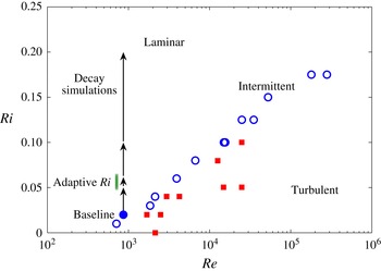
Reference Deusebio, Brethouwer, Schlatter and Lindborg2014; Deusebio, Caulfield & Taylor Reference Deusebio, Caulfield and Taylor2015). Figure 1 summarizes the simulations reported in Deusebio et al. (Reference Deusebio, Caulfield and Taylor2015), with blue circles used to indicate simulations with spatiotemporal intermittency and red squares used to indicate fully turbulent flow.
Flow regimes in stratified plane Couette flow as a function of Reynolds number,
 $Re$
, and Richardson number,
 $Ri$
. All simulations use a Prandtl number
 $Pr=0.7$
. The simulations reported in Deusebio et al. (Reference Deusebio, Caulfield and Taylor2015) are indicated with symbols. Blue circles denote simulations with spatiotemporal intermittency and red squares denote fully turbulent simulations. The solid blue circle is the baseline simulation described below in § 2.1. Arrows indicate an abrupt increase in
 $Ri$
at the start of each decay simulation described in § 2.2, and the green bar indicates the approximate range of
 $Ri$
seen in the adaptive simulations B, C and D, described in § 2.3.

Motivated by this, we use
 $Ri$
as a control parameter to study spatiotemporal intermittency using direct numerical simulations (DNS) of stratified plane Couette flow. For simplicity, we consider a single
 $Re$
, which is nearly three times larger than the critical value for unstratified plane Couette flow, and
 $Ri\in [0.02,0.2]$
: the baseline simulation with
 $Ri=0.02$
is indicated by a filled blue circle in figure 1. In the absence of stratification, flow at this
 $Re$
would be in the ‘featureless’ turbulence regime. However, stable stratification retards the transition process and the flow exhibits spatiotemporal intermittency in the form of patterned turbulence which will be described below. Note that most of the other simulations from Deusebio et al. (Reference Deusebio, Caulfield and Taylor2015) used a relatively small box size and were unable to distinguish between patterned and irregular intermittent turbulence.
The paper is organized as follows. In § 2.1, we briefly describe the numerical set-up and revisit one of the simulations reported in Deusebio et al. (Reference Deusebio, Caulfield and Taylor2015) in an intermittent regime, which we use as a baseline simulation. In § 2.2, we describe a series of decay simulations, each of which starts from an initial condition taken from the baseline simulation at
 $Ri=0.02$
. The decay simulations differ only in the new value of
 $Ri>0.02$
subsequently imposed. Section 2.3 then describes a novel strategy to isolate and stabilize a turbulent spot by turning on the dynamic adaptation of
 $Ri$
in the decay simulation for
 $Ri=0.05$
. The adaptive control procedure allows us to halt the decay process and isolate stripes and spots that characterize intermittent flows with a supercritical transition. Finally, we end with a brief summary and discussion in § 3.
2 Results
2.1 Set-up
Stratified plane Couette flow is bounded at the top and bottom by flat, rigid plates separated by a distance
 $2h$
. Here,
 $x$
,
 $y$
and
 $z$
will be used to denote the streamwise, wall-normal and spanwise directions, respectively, following the standard convention for Couette and channel flow. The plates move in opposite directions with constant velocity
 $\boldsymbol{u}=\pm U\hat{\boldsymbol{x}}$
. The walls are held at a fixed temperature,
 $\unicode[STIX]{x1D703}$
, such that the temperature of the upper wall is
 $2T$
higher than the temperature of the lower wall. Here, we consider the following non-dimensional incompressible Boussinesq equations with a linear equation of state:
 $$\begin{eqnarray}\displaystyle & \displaystyle \frac{\unicode[STIX]{x2202}\boldsymbol{u}}{\unicode[STIX]{x2202}t}+\boldsymbol{u}\boldsymbol{\cdot }\unicode[STIX]{x1D735}\boldsymbol{u}=-\unicode[STIX]{x1D735}p+Ri\unicode[STIX]{x1D703}\hat{\boldsymbol{y}}+\frac{1}{Re}\unicode[STIX]{x1D6FB}^{2}\boldsymbol{u}, & \displaystyle\end{eqnarray}$$
 $$\begin{eqnarray}\displaystyle & \displaystyle \frac{\unicode[STIX]{x2202}\unicode[STIX]{x1D703}}{\unicode[STIX]{x2202}t}+\boldsymbol{u}\boldsymbol{\cdot }\unicode[STIX]{x1D735}\unicode[STIX]{x1D703}=\frac{1}{RePr}\unicode[STIX]{x1D6FB}^{2}\unicode[STIX]{x1D703}, & \displaystyle\end{eqnarray}$$
 $$\begin{eqnarray}\displaystyle & \displaystyle \unicode[STIX]{x1D735}\boldsymbol{\cdot }\boldsymbol{u}=0, & \displaystyle\end{eqnarray}$$
where
 $$\begin{eqnarray}Re:=Uh/\unicode[STIX]{x1D708},\quad Ri:=|\boldsymbol{g}|\unicode[STIX]{x1D6FC}Th/U^{2},\quad Pr:=\unicode[STIX]{x1D708}/\unicode[STIX]{x1D705},\end{eqnarray}$$
 $\boldsymbol{g}=-g\hat{\boldsymbol{y}}$
is the acceleration due to gravity which acts in the
 $-y$
direction,
 $\unicode[STIX]{x1D708}$
is the kinematic viscosity,
 $\unicode[STIX]{x1D705}$
is the thermal diffusivity,
 $\unicode[STIX]{x1D6FC}$
is the thermal expansion coefficient, and
 $p$
is the non-dimensional pressure.
Periodic boundary conditions are applied in
 $x$
and
 $z$
. The numerical code uses a pseudo-spectral method in
 $x$
and
 $z$
and second-order finite differences to calculate derivatives in the
 $y$
direction. The time stepping algorithm is a mixed implicit/explicit scheme using the third-order Runge–Kutta and Crank–Nicolson methods. Further details of the problem configuration and numerical method can be found in Deusebio et al. (Reference Deusebio, Caulfield and Taylor2015).
One of the simulations reported by Deusebio et al. (Reference Deusebio, Caulfield and Taylor2015) is chosen as our ‘baseline’ simulation (filled blue circle in figure 1). This simulation has
 $Re=865$
,
 $Ri=0.02$
and
 $Pr=0.7$
. Although
 $Re$
is among the lowest considered by Deusebio et al. (Reference Deusebio, Caulfield and Taylor2015), it is still sufficiently high to be in the ‘fully turbulent’ regime for unstratified plane Couette flow (
 $Re\gtrsim 400$
) (Duguet et al.
Reference Duguet, Schlatter and Henningson2010). This case was chosen as our baseline since the modest resolution allows us to use a very large domain in the streamwise and spanwise directions, with
 $L_{x}=64\unicode[STIX]{x03C0}h$
and
 $L_{z}=32\unicode[STIX]{x03C0}h$
. The simulation uses 1024 gridpoints in the
 $x$
and
 $z$
directions and 64 points in
 $y$
, with gridpoints clustered near both walls. As discussed by Deusebio et al. (Reference Deusebio, Caulfield and Taylor2015), the large domain size reduces temporal intermittency of the flow and provides robust statistics.
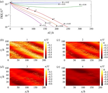
Figure 2(b) shows the streamwise velocity at
 $y=-0.5h$
, the horizontal plane half-way between the lower wall and the centreline. Turbulent and laminar regions develop in inclined bands reminiscent of those seen at lower Reynolds numbers in transitional plane Couette flow (Prigent et al.
Reference Prigent, Grégoire, Chaté, Dauchot and van Saarloos2002). Deusebio et al. (Reference Deusebio, Caulfield and Taylor2015) described a method for identifying local turbulent and laminar regions and defined the ‘turbulent fraction’,
 $\unicode[STIX]{x1D6FE}$
, as the fraction of the total domain occupied by turbulent flow. For sufficiently large
 $Re$
and small
 $Ri$
, the flow is fully turbulent with
 $\unicode[STIX]{x1D6FE}=1$
(red squares in figure 1). For sufficiently small
 $Re$
and large
 $Ri$
, intermittent flow is seen with
 $0<\unicode[STIX]{x1D6FE}<1$
(blue circles in figure 1). For the baseline simulation,
 $\unicode[STIX]{x1D6FE}=0.64$
(solid circle in figure 1).
2.2 Decay simulations
In the first set of simulations, we varied the strength of the stable stratification by abruptly increasing
 $Ri$
. Each simulation was initialized from the baseline simulation described above with
 $Re=865$
and
 $Ri=0.02$
with a state obtained at statistical equilibrium. The decay simulations are indicated in figure 1 as vertical arrows ending at the new Richardson number. For convenience,
 $t=0$
will correspond to the time when
 $Ri$
is abruptly increased. Since
 $Ri$
multiplies the buoyancy term in the non-dimensional vertical momentum equation, increasing
 $Ri$
is equivalent to increasing the gravitational acceleration, i.e. heavy fluid becomes heavier and light fluid becomes lighter.
Figure 2(a) shows the time evolution of the turbulent kinetic energy,
 $\mathit{TKE}:=\langle \boldsymbol{u}^{\prime }\boldsymbol{\cdot }\boldsymbol{u}^{\prime }\rangle /2$
, where
 $\langle \cdot \rangle$
denotes a volume average and primes denote a departure from this average, i.e.
 $\boldsymbol{u}^{\prime }:=\boldsymbol{u}-\langle \boldsymbol{u}\rangle$
. In four cases with
 $Ri\geqslant 0.05$
, the TKE decays in time at an approximately exponential rate, and the rate of decay increases with
 $Ri$
. Eventually all simulations with
 $Ri\geqslant 0.05$
reach a fully laminar state. When
 $Ri=0.03$
and
 $Ri=0.04$
, the TKE decays during a transient period and partially recovers, but remains below the initial value. For comparison, a continuation of the baseline case with
 $Ri=0.02$
is also shown.
(a) Time series of the turbulent kinetic energy (TKE) in the decay simulations. Each simulation starts from the same initial state labelled 1. The Richardson number in each simulation is labelled. (b)–(e) Horizontal slices of the streamwise velocity at
 $y=-0.5h$
at various times in the simulation with
 $Ri=0.05$
. The corresponding times are indicated with dots and numbered in panel (a). The first time (b) shows the velocity in the baseline simulation that was used to initialize the decay simulations. In this simulation spatiotemporal intermittency takes the form of a repeating pattern of bands (or stripes) of turbulence inclined with respect to the spanwise direction.

The decay process does not proceed uniformly in space, but instead turbulence persists in localized ‘pockets’ contained within receding turbulent bands, qualitatively similar to what has been seen in previous simulations of decaying unstratified turbulence (Manneville Reference Manneville2011). Figure 2(b)–(e) shows four snapshots of the streamwise velocity at
 $y=-0.5h$
in the decay simulation with
 $Ri=0.05$
. The corresponding times are indicated using dots in figure 2(a). Highly localized patches of turbulence can be seen at times labelled
 $3$
and
 $4$
, while the rest of the flow is nearly laminar.
2.3 Adaptive Ri simulations
In order to examine further the influence of stratification on the flow near the laminar–turbulent transition, we have developed a procedure using the Richardson number,
 $Ri$
, as an adaptive control parameter. To our knowledge, this is the first time that
 $Ri$
has been used to control the level of turbulence in a stratified flow. The procedure allows us to isolate turbulent states progressively closer to the relaminarization boundary. The adaptive procedure changes
 $Ri$
based on the rate of change of TKE. Let
 $t_{0}$
correspond to the time
 $M$
time steps before the current time,
 $t$
, and let
 $\mathit{TKE}(t_{0})$
and
 $\mathit{TKE}(t)$
be the TKE at these times. The TKE decay time scale,
 $\unicode[STIX]{x1D70F}$
, between times
 $t_{0}$
and
 $t$
is
 $$\begin{eqnarray}\unicode[STIX]{x1D70F}:=\frac{-(t-t_{0})}{\displaystyle \ln \!\left(\frac{\mathit{TKE}(t)}{\mathit{TKE}(t_{0})}\right)}\end{eqnarray}$$
and the Richardson number,
 $Ri(t)$
, is then set as
 $$\begin{eqnarray}Ri(t):=Ri(t_{0})-c\frac{t-t_{0}}{\unicode[STIX]{x1D70F}},\end{eqnarray}$$
where
 $Ri(t_{0})$
was the previous value at
 $t_{0}$
, and
 $c$
is a control parameter that will be discussed later. The adaptive
 $Ri$
procedure acts to maintain a roughly constant value of the TKE. The turbulent fraction and TKE level are sensitive to
 $Ri$
(Deusebio et al.
Reference Deusebio, Caulfield and Taylor2015). During periods where TKE decreases in time (
 $\unicode[STIX]{x1D70F}>0$
), the adaptive procedure will decrease
 $Ri$
, which has the ultimate effect of increasing the TKE, thus leading to the possibility of ‘controlling’ the turbulence at a non-trivial level. Mathematically, if
 $Ri$
was adjusted every time step, equations (2.5) and (2.6) are a finite difference approximation to imposing the extra dynamical constraint
 $$\begin{eqnarray}\frac{\text{d}}{\text{d}t}\left[Ri(t)+c\ln \!\left(\frac{\mathit{TKE}}{\mathit{TKE}_{0}}\right)\right]=0,\end{eqnarray}$$
to the Boussinesq equations and
 $TKE_{0}$
is an arbitrary constant energy. Note that
 $c=0$
recovers the Boussinesq equations with constant
 $Ri$
.
In the adaptive
 $Ri$
simulations, we updated
 $Ri$
using (2.6) every
 $M=20$
time steps and set
 $c=0.1$
. The value of
 $M$
was chosen to reduce the computational cost of this procedure while ensuring that
 $Ri$
is adjusted sufficiently often to keep pace with any change in the TKE decay rate. In practice, the time between
 $Ri$
adjustment steps is always less than one advective unit,
 $t-t_{0}<h/U$
. The sensitivity of the results to the choice of
 $c$
will be examined later. We have used the adaptive
 $Ri$
procedure to isolate turbulent states during various stages of the decay process. We saved three-dimensional flow fields at various times during the decay simulation with
 $Ri=0.05$
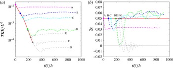
, indicated by dots in figure 3(a). Each of these was then used as an initial condition for an adaptive
 $Ri$
simulation. To ensure continuity,
 $Ri$
was initialized to 0.05 in the adaptive
 $Ri$
simulations.
Time series of the TKE from the adaptive
 $Ri$
simulations are shown in dashed lines in figure 3(a). The decay simulation with
 $Ri=0.05$
is shown for reference (solid line). The simulations with adaptive
 $Ri$
are each labelled with a letter (A–G). In simulations labelled A–D, the TKE continues to decrease at the start of the adaptive simulation, but soon reaches a quasi-steady state. Simulations initialized later in the decay process have quasi-steady states with lower TKE. Time series of
 $Ri$
in the adaptive simulations are shown in figure 3(b). In all cases
 $Ri$
reaches a quasi-steady state after an initial drop – mirroring the TKE. Interestingly, the quasi-steady value of
 $Ri$
in cases B, C and D falls in the same range,
 $Ri\simeq 0.05{-}0.06$
, despite very different values of the TKE in these simulations. Simulation A has a smaller quasi-steady value of
 $Ri\simeq 0.03$
. For context, the approximate range of
 $Ri$
in the quasi-steady state for simulations B, C and D is indicated as a green band in figure 1.
(a) Time series of the turbulent kinetic energy (TKE) in the adaptive
 $Ri$
simulations. The simulations are initialized from various times in the
 $Ri=0.05$
decay simulations as indicated by coloured dots. (b) Time series of the Richardson number,
 $Ri$
, for each of the adaptive
 $Ri$
simulations using the control scheme described in the text. The solid red line indicates
 $Ri=0.05$
from the decay simulation. The start time of each simulation is indicated with a coloured dot, and the colours and labels are the same as in panel (a).

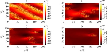
Horizontal slices of the streamwise velocity at
 $y=-0.5h$
at the end of the adaptive
 $Ri$
simulations. Labels are the same as in figure 3.

Simulation D is the lowest level of TKE that we have been able to reach using this procedure. In simulations E–G, the flow nearly relaminarizes during the adaptive
 $Ri$
simulation. In this regime,
 $Ri$
oscillates and eventually becomes negative (figure 3
b), while the flow develops into a series of streamwise-independent rolls (not shown) corresponding closely to slightly supercritical, sheared Rayleigh–Bénard convection (Clever, Busse & Kelly Reference Clever, Busse and Kelly1977; Kelly Reference Kelly1977). There are dramatic differences in the character of the flow and the value of the steady-state
 $Ri$
in simulations D and E, implying that the flow in simulation D is close to the relaminarization boundary.
The streamwise velocity at
 $y=-0.5h$
is shown for four adaptive
 $Ri$
simulations in figure 4. Each snapshot corresponds to the end of the adaptive
 $Ri$
simulation, as labelled in figure 3(a). Simulation A was initialized directly from the baseline simulation (magenta dot) with
 $Ri=0.05$
and the TKE decreases slightly at the start of the simulation. Turbulent/laminar bands are still prominent features of simulation A, and the laminar regions are more coherent than in the baseline simulation (compare figure 2
b and figure 4 simulation A). In the other extreme, simulation D has a single turbulent spot. This spot persists throughout the adaptive
 $Ri$
simulation, slowly migrating around the domain. Simulations B and C have multiple turbulent spots resembling the one seen in simulation D. In simulation B some of the spots appear to join together, with some indications of short inclined bands of turbulence.
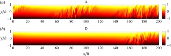
The turbulent structures in the isolated turbulent spot are qualitatively similar to the structures in the turbulent stripes. Figure 5 shows vertical slices of the temperature field from simulations A and D illustrating these two regimes. Turbulence in the stripes and spot spans the gap between the lower and upper plates, and is inclined in the direction of plate motion. Small regions with an unstable density arrangement (heavy over light) occur in the turbulent patch. Features reminiscent of developing Kelvin–Helmholtz billows appear on the flanks of the turbulent patches, for example between
 $60\leqslant x/h\leqslant 80$
in simulation A and
 $150\leqslant x/h\leqslant 170$
in simulation D (note that the aspect ratio is highly stretched).


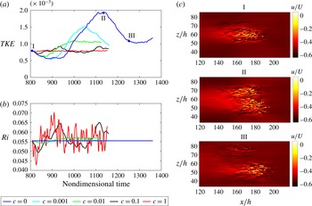
To examine the sensitivity of our results to details of the adaptive
 $Ri$
procedure, we continued simulation D (exhibiting a single turbulent spot) with various values of the adjustment coefficient,
 $c$
, including a case with
 $c=0$
when
 $Ri$
is held fixed. Time series of the TKE and
 $Ri$
are shown in figure 6. When
 $c=1$
, the TKE remains close to constant in time, but
 $Ri$
exhibits large, high-frequency oscillations. In contrast, when
 $Ri$
is held fixed (
 $c=0$
), the TKE undergoes large low-frequency oscillations in time. In this uncontrolled simulation the turbulent spot first grows, splits into two spots, and one of these spots decays (figure 6
c). The remaining spot looks remarkably similar to the controlled spot from which the simulation was started, more than 400 advective time units earlier (compare times labelled I and III). This suggests that the controlled spot is at least qualitatively representative of the uncontrolled system. The intermediate values,
 $c=0.1$
and
 $c=0.01$
, represent a trade-off between larger oscillations in
 $Ri$
and TKE, respectively.
Dependence of the TKE (a) and Richardson number (b) on the choice of the coefficient,
 $c$
, in (2.6). Each simulation is started from the end of simulation D with a single controlled turbulent spot. (c) Visualizations of the streamwise velocity from an uncontrolled simulation (
 $c=0$
) are shown for the times indicated in blue dots in panel (a).

A natural question to ask is whether the captured turbulent spot obtained using the adaptive control procedure is sensitive to the initial conditions. That is, does the flow retain some ‘memory’ of the simulation with decaying stratified turbulence from which it was started? To address this question, we ran an additional simulation initialized with a localized ‘seed’ following the procedure of Lagha & Manneville (Reference Lagha and Manneville2007). Specifically, we started with the velocity from a simulation of unstratified plane Couette flow at the same Reynolds number in the featureless turbulence regime. The initial velocity was then formed by multiplying the unstratified velocity field by a Gaussian function of
 $x$
and
 $z$
,
 $$\begin{eqnarray}\boldsymbol{u}(\boldsymbol{x},t=0)=\boldsymbol{u}_{Ri=0}(\boldsymbol{x})\text{e}^{-(x^{2}+z^{2})/S},\end{eqnarray}$$
where
 $S=2h^{2}$
. Note that this seed is significantly smaller than the turbulent spot seen in simulation D. The seed was allowed to develop with
 $Ri=0$
for 35 advective time units, after which point, the adaptive procedure was started with
 $c=0.1$
. Although the Richardson number was started from
 $Ri=0$
, it converged towards approximately the same value seen in simulations B, C and D, and the flow developed into a single turbulent spot that appeared extremely similar in structure to the one in simulation D. This result implies that the turbulent spot is not sensitive to the initialization procedure. When the adaptive procedure was started without first allowing the seed to grow, the increase in stratification caused the flow to relaminarize. This supports the idea that the turbulent spot captured in simulation D is close to the minimal energy turbulent attractor, the lowest-energy turbulent state that can be maintained using the adaptive
 $Ri$
procedure.
3 Discussion
We have examined intermittent stratified plane Couette flow using direct numerical simulations. While the Reynolds number was kept fixed, the Richardson number,
 $Ri$
, was used as a control parameter, allowing us to probe the dynamics of intermittent stratified turbulence in this geometry. We have considered two sets of simulations. In the first set of simulations,
 $Ri$
is abruptly increased relative to a control simulation. For sufficiently large values of
 $Ri$
, the flow relaminarizes. However, in these simulations, localized patches of turbulence persist into the decay period until the flow becomes fully laminar. This result is qualitatively similar to Manneville (Reference Manneville2011), who found breakup of turbulent bands in decaying unstratified plane Couette flow.
Next, we describe a new method to isolate flow structures at very low turbulent energy using
 $Ri$
as an adaptive control parameter. The method adjusts
 $Ri$
based on the time rate of change in the turbulent kinetic energy (TKE), increasing
 $Ri$
when the TKE is increasing and lowering
 $Ri$
when the TKE is decreasing. The adaptive control procedure acts to stabilize the flow close to the initial energy level. By starting the adaptive procedure at various times during a simulation of decaying stratified turbulence, we are able to isolate a variety of low-energy flow structures, including spots and short stripes of turbulence.
When the Richardson number changes through the control procedure introduced here, the buoyancy of the fluid changes everywhere in the domain instantaneously. It is difficult to imagine a means to change the density of a real fluid in a similar way by changing its temperature or salinity. However, a change in buoyancy could be interpreted as a change in the gravitational acceleration. An analogue laboratory experiment would measure the change in TKE within a given time window and accelerate the entire Couette flow apparatus up or down so as to change the fluid buoyancy instantaneously everywhere throughout the flow. Although it would be difficult to implement this system in a practical laboratory experiment, it provides a physical interpretation of the control procedure.
The lowest-energy turbulent structure that we are able to identify using the adaptive control procedure consists of a single isolated turbulent spot in an otherwise laminar flow. Qualitatively, this stabilized spot is very similar to the spots seen previously in unstratified transitional flows, and it seems reasonable to assume that they are closely related. Studying this stabilized spot then offers an exciting opportunity to probe the dynamics seen. However, confirming a connection is not as simple as examining the
 $c\rightarrow 0$
limit, because the fluctuations in energy become larger as
 $c$
decreases, until eventually the spot becomes uncontrollable at some small but finite
 $c$
(see figure 6).
The scheme to adapt
 $Ri$
based on the time rate of change of
 $TKE$
is somewhat arbitrary, and other choices could be made. For example, it might be possible to control a turbulent spot in unstratified flow using the Reynolds number as a control parameter. One could use this technique to explore the dynamics of multiple interacting controlled spots. For example, if a simulation were initialized with several isolated turbulent spots, would they coalesce into stripes and eventually form patterns? If so, do the properties of the turbulent spot provide insight into properties of patterned turbulence such as the width of the turbulent bands?
Another interesting issue is how the stabilized spot in the controlled system – the Boussinesq equations augmented by the constraint (2.7)) with
 $Ri(t)$
now a dynamic variable – is related to the laminar–turbulent boundary or ‘edge’ (Itano & Toh Reference Itano and Toh2001; Skufca, Yorke & Eckhardt Reference Skufca, Yorke and Eckhardt2006) in the uncontrolled Boussinesq equations with, say, the required fixed value of
 $Ri$
defined as
 $\overline{Ri}$
, the long-time average of
 $Ri(t)$
(a reasonable but not unique choice to link the controlled system with variable
 $Ri(t)$
and the uncontrolled system with fixed
 $Ri$
). In the controlled system, the spot is a stable low-energy state and must therefore sit ‘above’ the edge (i.e. not in the laminar basin of attraction) but presumably still close to it. The edge for the controlled system has an extra dimension in phase space compared to that for the uncontrolled system due to
 $Ri(t)$
being an extra dynamic variable. Projecting the edge in the controlled system down onto the hyperplane with fixed
 $Ri=\overline{Ri(t)}$
might produce a good estimate for the edge in the uncontrolled system provided the fluctuations in
 $Ri(t)$
are not too large compared to
 $\overline{Ri(t)}$
. However, it is unclear where the projected stabilized spot solution will land in phase space relative to the uncontrolled system edge: i.e. it could be inside, outside or even on it, and so the control procedure is not a direct competitor to bisection-based edge tracking (Itano & Toh Reference Itano and Toh2001; Skufca et al.
Reference Skufca, Yorke and Eckhardt2006), which endeavours to work on the edge.
In this paper we have only considered a single Reynolds number,
 $Re=Uh/\unicode[STIX]{x1D708}=865$
. Although this Reynolds number is large enough to support fully developed turbulence in the unstratified limit, it is much smaller than typical values in geophysical and industrial flows. One consequence of the moderate Reynolds number is that the Richardson number associated with intermittent flow is also modest. Deusebio et al. (Reference Deusebio, Caulfield and Taylor2015) found intermittent behaviour at much higher Reynolds numbers for sufficiently large Richardson number, which is also consistent with previous work (e.g. Flores & Riley Reference Flores and Riley2010; García-Villalba & del Álamo Reference García-Villalba and del Álamo2011; Brethouwer et al.
Reference Brethouwer, Duguet and Schlatter2012). The fate of the laminar–turbulent transition boundary in the limit as
 $Re\rightarrow \infty$
is one of the most important open problems in stratified turbulence. Knowing whether there is a finite ‘critical’ value of
 $Ri$
above which turbulence cannot persist as
 $Re\rightarrow \infty$
would be of great use in parameterizing turbulence and mixing in ocean, atmosphere, and climate models.
One of the difficulties with answering this question is the rapid increase in computational cost with increasing
 $Re$
. Very close to the transition boundary, where stratification suppresses energetic turbulence and localizes turbulent patches, the flow might be more accessible to DNS. However, this accessible region narrows in parameter space as
 $Re\rightarrow \infty$
(Deusebio et al.
Reference Deusebio, Caulfield and Taylor2015), making it difficult to locate the transition boundary. Here, too, our adaptive control technique might be helpful, since the long-time average of
 $Ri(t)$
needed to maintain a low perturbation energy level as
 $Re$
increases should be a good predictor for this boundary.
Acknowledgements
The EPSRC grant EP/K034529/1 entitled ‘Mathematical Underpinnings of Stratified Turbulence’ is gratefully acknowledged for supporting the research presented here. We thank P. F. Linden, S. B. Dalziel and the rest of the MUST team for many helpful discussions. We also thank three anonymous referees for their helpful comments. Data for the initial conditions and simulation output are made available at https://doi.org/10.17863/CAM.5913.