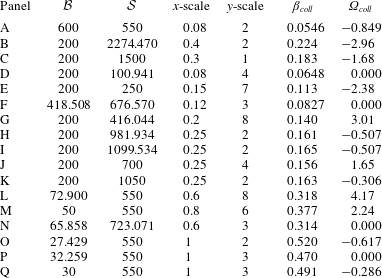
1 Introduction
The tendency of thin liquid films to destabilize and form wavy patterns is an important area of research for a wide range of applications. For some applications, such as coatings and glass manufacturing, one may wish to operate under conditions that avoid these instabilities. In others, such as multiphase heat/mass transfer technology and nanoscale patterning of liquid metals/polymers, precise control of the emerging wave pattern is of utmost concern. In either case, the parametric conditions of interest can be determined, most simply, by applying the long-wave approximation to the governing nonlinear equations, see Oron, Davis & Bankoff (Reference Oron, Davis and Bankoff1997) and Craster & Matar (Reference Craster and Matar2009). In the long-wave approach, physical effects such as gravity, mean surface tension, thermocapillarity, solutocapillarity and electromagnetism can be easily be accounted for, and one typically obtains a single nonlinear partial differential equation (PDE) for the spatio-temporal evolution of the local film thickness. This method assumes the film dynamics is non-inertial and governed by a (first order in time) nonlinear PDE.
The principal phenomenon that a single-equation long-wave model cannot describe is the emergence of instabilities that are oscillatory in time, i.e. overstability (see Nepomnyashchy, Velarde & Colinet (Reference Nepomnyashchy, Velarde and Colinet2001), chapter 5). Whereas single-equation film models predict monotonic perturbations that grow or decay exponentially in time, oscillatory instabilities can only be observed in systems that describe the interaction between processes that occur on distinct time scales. Thus, oscillatory instabilities are commonly obtained from Orr–Sommerfeld type analyses of governing equations of motion that retain inertial effects and diffusive time scales. Wide-ranging examples that highlight the emergence of oscillatory instabilities in fluid layers include work by Sternling & Scriven (Reference Sternling and Scriven1959), Takashima (Reference Takashima1981), Anderson & Worster (Reference Anderson and Worster1996) and Rednikov et al. (Reference Rednikov, Colinet, Velarde and Legros1998). A common theme to these works is the level of analytical difficulty; each obtains a linear dispersion relation (describing system stability) that is transcendental and implicit in the perturbation growth rates. Combined with large parametric spaces and the fact that oscillatory perturbations necessarily reside in the complex plane, concise description of the emergence of oscillatory instability can be a challenging task. Alternatively, the long-wave approximation offers a convenient means to couple free surface deformation to other time-dependent physical processes of interest.
Several authors have investigated oscillatory instabilities of thin liquid films in the context of the long-wave approximation. In many cases, e.g. Podolny, Oron & Nepomnyashchy (Reference Podolny, Oron and Nepomnyashchy2005) and Bestehorn & Borcia (Reference Bestehorn and Borcia2010), such instabilities originate from the coupling between the local thickness and bulk concentration of a film composed of a binary mixture. In addition to the bulk concentration dynamics, Morozov, Oron & Nepomnyashchy (Reference Morozov, Oron and Nepomnyashchy2014) investigated oscillatory instability with the added effect of absorption/desorption kinetics between interfacial and bulk film surfactant concentration. In other cases, oscillatory instabilities have been uncovered in multiple stacked layers of films, as described theoretically by coupled sets of film thickness evolution equations (Beerman & Brush Reference Beerman and Brush2007; Nepomnyashchy & Simanovskii Reference Nepomnyashchy and Simanovskii2007). Multi-layer film configurations do not, however, guarantee oscillatory modes: for example, such instabilities were not obtained by Pototsky et al. (Reference Pototsky, Bestehorn, Merkt and Thiele2005) who investigated the dewetting dynamics of isothermal, ultra-thin bilayers. Of particular interest to the present work are oscillatory instabilities reported by Shklyaev, Alabuzhev & Khenner (Reference Shklyaev, Alabuzhev and Khenner2012) in a model of thin-film thermocapillary destabilization from below. While there are similarities between that work and the present, we point out one important difference: in Shklyaev et al. (Reference Shklyaev, Alabuzhev and Khenner2012), the instability is driven by imposing a heat flux at the film–substrate interface; instead, in the present work we obtain oscillatory instabilities by coupling film dynamics to a thermally diffusive, two-dimensional substrate. We also note that each of these works on oscillatory instabilities of thin liquid films obtains low-order polynomial equations for the perturbation growth rates (in contrast to the transcendental, implicit dispersion we obtain in the present work).
The problem we investigate in this work is the deformational thermocapillary instability. This classic long-wavelength instability was first introduced by Scriven & Sternling (Reference Scriven and Sternling1964) and later verified experimentally by VanHook et al. (Reference VanHook, Schatz, Swift, McCormick and Swinney1997). In short, thermocapillary stresses that destabilize the free surface are generated by heating a film from below (normal heating). For sufficiently thin layers, these stresses can surpass capillary stabilization and deform an initially flat film. Recently, Dietzel & Troian (Reference Dietzel and Troian2009) connected this mechanism with the formation of nanopillars (
 ${\sim}10~\unicode[STIX]{x03BC}\text{m}$
spacing) on ultrathin (
 ${\sim}100$
nm) polymer films. Continuing work on thermocapillary patterning in (ultra)thin polymer films has been reviewed by Singer (Reference Singer2017). A patterning application that directly motivates our study is pulsed-laser dewetting of nanometric liquid metal films. Experiments by Trice et al. (Reference Trice, Thomas, Favazza, Sureshkumar and Kalyanaraman2007) demonstrated dewetting pattern wavelengths that were commensurate with the predictions of long-wavelength thermocapillary modes. Driven by such results, several workers have developed and investigated theoretical models for the pulsed-laser process. Atena & Khenner (Reference Atena and Khenner2009) augmented a long-wave theory with pulsed laser irradiation to describe the thermocapillary dewetting of liquid cobalt on silicon oxide substrates. Notably, they assumed that the substrate was thin, thereby ensuring the model dynamics could be described by a (first order in time) single nonlinear PDE for the film thickness. As a result, oscillatory instabilities do not arise in their model.
Recently, oscillatory modes for pulsed-laser thermocapillary dewetting of liquid metal films were uncovered by Dong & Kondic (Reference Dong and Kondic2016) and Seric, Afkhami & Kondic (Reference Seric, Afkhami and Kondic2018). These authors made observations primarily via nonlinear simulations of a model that couples the film PDE to the full heat equation for the substrate. These works have not precisely characterized the emergence of oscillatory instabilities, in particular, because the task is further complicated by the parameter space that arises for laser heating. Thus, in the present work, we investigate the emergence of oscillatory instability for the simpler problem: a film heated by a thick solid substrate. To do so, we initially follow the work by Saeki, Fukui & Matsuoka (Reference Saeki, Fukui and Matsuoka2011, Reference Saeki, Fukui and Matsuoka2013) that considered the linear analysis of a coupled film–substrate model, which induces thermocapillary film deformation driven by laser heating. In the present work we follow their asymptotic assumptions so that the full heat equation of the substrate is retained at leading order in the long-wave expansion of the governing equations. Effectively, we assume that the substrate–film thermal conductivity and thickness ratios are large. Although we obtain a dispersion relation that is similar to that of Saeki et al. (Reference Saeki, Fukui and Matsuoka2013), it is important to note that they did not observe oscillatory modes. This may be due to a limited examination of model parameter values in their investigation.
The manuscript proceeds as follows: in § 2 we present the dimensional equations of motion and boundary conditions for a deformable liquid layer heated by a thick substrate. In § 3 we introduce a long-wave asymptotic expansion and derive an evolution equation for the film thickness that is non-locally coupled to the diffusive (time-dependent) heat conduction problem in the substrate. In this section we also introduce a unique non-dimensionalization that casts the non-local model in terms of four dimensionless parameters: (i)
 ${\mathcal{B}}$
, characterizing the mean thermal thickness of the film; (ii)
 ${\mathcal{S}}$
, characterizing the thermal thickness of the substrate; (iii)
 ${\mathcal{C}}$
, characterizing the imposed temperature difference; (iv)
 ${\mathcal{Q}}$
, depending only on material properties. In the following section, § 4, we perform a linear analysis of the non-local model and demonstrate that its stability is governed by a generalized two-point boundary value problem that is not self-adjoint. Solution of this problem yields the (implicit) dispersion relation that sets the course of investigation for the remainder of the paper. In § 5 we characterize the root structure of the dispersion relation and introduce the numerical continuation methods we use to track its roots as functions of the perturbation wavenumbers. Then, in § 6 we classify the two characteristic pathways by which oscillatory instability manifests itself. In § 7 we provide a complete picture of the emergence of oscillatory instabilities within the considered parameter space. Finally, in § 8 we discuss application of our model to practical settings and offer suggestions for future work.
2 Dimensional equations
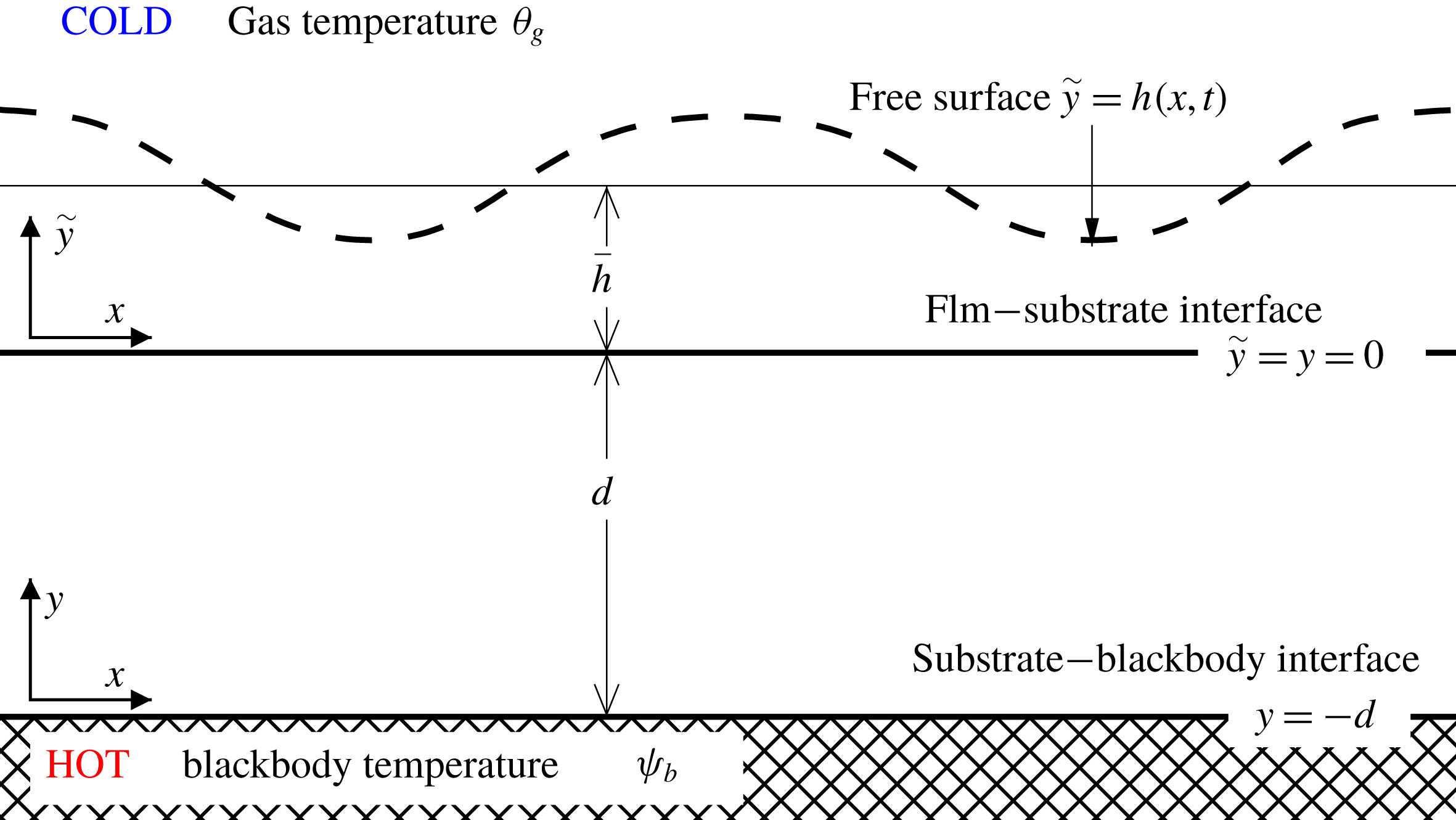
Here we introduce equations that describe the fluid and temperature dynamics of the laterally infinite, two-dimensional film–substrate system depicted schematically in figure 1. The film is composed of a Newtonian, incompressible liquid with average thickness
 $\overline{h}$
, density
 $\unicode[STIX]{x1D70C}$
, dynamic viscosity
 $\unicode[STIX]{x1D707}$
, kinematic viscosity
 $\unicode[STIX]{x1D708}=\unicode[STIX]{x1D707}/\unicode[STIX]{x1D70C}$
, thermal conductivity
 $\unicode[STIX]{x1D705}_{f}$
and thermal diffusivity
 $\unicode[STIX]{x1D712}_{f}$
. Neglecting gravity, we have
 $$\begin{eqnarray}\displaystyle & \displaystyle \unicode[STIX]{x1D70C}\left(\unicode[STIX]{x2202}_{t}\boldsymbol{v}+\boldsymbol{v}\boldsymbol{\cdot }\unicode[STIX]{x1D735}\boldsymbol{v}\right)=-\unicode[STIX]{x1D735}p+\unicode[STIX]{x1D707}\unicode[STIX]{x1D6FB}^{2}\boldsymbol{v}, & \displaystyle\end{eqnarray}$$
 $$\begin{eqnarray}\displaystyle & \displaystyle \unicode[STIX]{x1D735}\boldsymbol{\cdot }\boldsymbol{v}=0, & \displaystyle\end{eqnarray}$$
 $$\begin{eqnarray}\displaystyle & \displaystyle \unicode[STIX]{x2202}_{t}\unicode[STIX]{x1D703}+\boldsymbol{v}\boldsymbol{\cdot }\unicode[STIX]{x1D735}\unicode[STIX]{x1D703}=\unicode[STIX]{x1D712}_{f}\unicode[STIX]{x1D6FB}^{2}\unicode[STIX]{x1D703}, & \displaystyle\end{eqnarray}$$
where
 $\boldsymbol{v}\equiv \{u(x,{\tilde{y}},t),w(x,{\tilde{y}},t)\}$
,
 $p(x,{\tilde{y}},t)$
and
 $\unicode[STIX]{x1D703}(x,{\tilde{y}},t)$
are the film velocity, pressure and temperature fields, respectively. With
 $\unicode[STIX]{x1D735}=\{\unicode[STIX]{x2202}_{x},\unicode[STIX]{x2202}_{{\tilde{y}}}\}$
, equations (2.1)–(2.3) govern the evolution of these fields in time
 $t$
on the horizontal range
 $x\in (-\infty ,\infty )$
and the vertical range
 ${\tilde{y}}\in [0,h]$
where
 $h=h(x,t)$
is the local, instantaneous film thickness.
Geometric sketch of the problem.

The dynamics of this system is decoupled from that of the gas phase by assuming that the ratios between the liquid and gas phase densities, viscosities and thermal diffusivities are large. Accordingly, at the free surface, we have the kinematic condition
 $$\begin{eqnarray}\unicode[STIX]{x2202}_{t}h+\boldsymbol{v}\boldsymbol{\cdot }\unicode[STIX]{x1D735}h=w\quad \text{at }{\tilde{y}}=h,\end{eqnarray}$$
which states that the speed of the free surface is equal to the velocity of the fluid. Using
 $$\begin{eqnarray}\unicode[STIX]{x1D703}_{h}=\unicode[STIX]{x1D703}_{h}(x,t)\equiv \unicode[STIX]{x1D703}(x,h,t),\end{eqnarray}$$
to denote the free surface temperature, the normal and tangential stress balances that hold at the free surface are
 $$\begin{eqnarray}\displaystyle & \displaystyle p_{g}-p+\unicode[STIX]{x1D64F}\boldsymbol{\cdot }\boldsymbol{n}\boldsymbol{\cdot }\boldsymbol{n}=-2{\mathcal{H}}\unicode[STIX]{x1D70E}(\unicode[STIX]{x1D703}_{h})\quad \text{at }{\tilde{y}}=h, & \displaystyle\end{eqnarray}$$
 $$\begin{eqnarray}\displaystyle & \displaystyle \unicode[STIX]{x1D64F}\boldsymbol{\cdot }\boldsymbol{n}\boldsymbol{\cdot }\boldsymbol{t}=\unicode[STIX]{x1D735}\unicode[STIX]{x1D70E}(\unicode[STIX]{x1D703}_{h})\boldsymbol{\cdot }\boldsymbol{t}\quad \text{at }{\tilde{y}}=h, & \displaystyle\end{eqnarray}$$
respectively, with gas pressure
 $p_{g}$
, rate of deformation tensor
 $\unicode[STIX]{x1D64F}=\unicode[STIX]{x1D707}[\unicode[STIX]{x1D735}\boldsymbol{v}+(\unicode[STIX]{x1D735}\boldsymbol{v})^{\intercal }]$
in the liquid phase, surface normal and tangent unit vectors,
 $$\begin{eqnarray}\boldsymbol{n}=\frac{\boldsymbol{k}-\unicode[STIX]{x2202}_{x}h\boldsymbol{i}}{\sqrt{1+(\unicode[STIX]{x2202}_{x}h)^{2}}}\quad \boldsymbol{t}=\frac{\boldsymbol{i}+\unicode[STIX]{x2202}_{x}h\boldsymbol{k}}{\sqrt{1+(\unicode[STIX]{x2202}_{x}h)^{2}}},\end{eqnarray}$$
and twice mean curvature
 $2{\mathcal{H}}=-\unicode[STIX]{x1D735}\boldsymbol{\cdot }\boldsymbol{n}$
. We consider fluids whose surface tension decreases linearly with temperature according to
 $\unicode[STIX]{x1D70E}(\unicode[STIX]{x1D703}_{h})=\unicode[STIX]{x1D70E}_{0}-\unicode[STIX]{x1D6FE}(\unicode[STIX]{x1D703}_{h}-\unicode[STIX]{x1D703}_{0})$
where
 $\unicode[STIX]{x1D6FE}=-\text{d}\unicode[STIX]{x1D70E}/\text{d}\unicode[STIX]{x1D703}_{h}$
is positive and
 $\unicode[STIX]{x1D703}_{0}$
is a reference temperature.
Variations in
 $\unicode[STIX]{x1D703}_{h}$
leading to thermocapillary destabilization are driven by the heat exchanged with the bounding gas phase. This process is modelled using Newton’s law of cooling, viz.,
 $$\begin{eqnarray}\unicode[STIX]{x1D705}_{f}\unicode[STIX]{x1D735}\unicode[STIX]{x1D703}\boldsymbol{\cdot }\boldsymbol{n}+q\left(\unicode[STIX]{x1D703}_{h}-\unicode[STIX]{x1D703}_{g}\right)=0\quad \text{at }{\tilde{y}}=h,\end{eqnarray}$$
where
 $\unicode[STIX]{x1D703}_{g}$
is the uniform gas temperature and
 $q$
is the empirical rate of heat transfer between the surface and the gas.
The film temperature evolves according to (2.3), and, at
 $y=0$
, the film is in thermal contact with a rigid substrate of temperature
 $\unicode[STIX]{x1D713}$
, thermal conductivity
 $\unicode[STIX]{x1D705}_{s}$
and diffusivity
 $\unicode[STIX]{x1D712}_{s}$
. No slip and no penetration enforce
 $\boldsymbol{v}=\mathbf{0}$
, and, continuity of temperature and heat flux requires
 $$\begin{eqnarray}\displaystyle & \displaystyle \unicode[STIX]{x1D703}=\unicode[STIX]{x1D713}\quad \text{at }{\tilde{y}}=y=0, & \displaystyle\end{eqnarray}$$
 $$\begin{eqnarray}\displaystyle & \displaystyle \unicode[STIX]{x2202}_{{\tilde{y}}}\unicode[STIX]{x1D703}=\unicode[STIX]{x1D705}\,\unicode[STIX]{x2202}_{y}\unicode[STIX]{x1D713}\quad \text{at }{\tilde{y}}=y=0, & \displaystyle\end{eqnarray}$$
where
 $$\begin{eqnarray}\displaystyle \unicode[STIX]{x1D705}=\unicode[STIX]{x1D705}_{s}/\unicode[STIX]{x1D705}_{f} & & \displaystyle\end{eqnarray}$$
is the conductivity ratio. Here, the vertical domain of
 $\unicode[STIX]{x1D713}$
is assigned to a second vertical coordinate
 $z\in [-d,0]$
in anticipation that two vertical length scales will be introduced in the asymptotic analysis of the thick substrate case. The evolution of
 $\unicode[STIX]{x1D713}$
throughout the substrate is governed by
 $$\begin{eqnarray}\unicode[STIX]{x2202}_{t}\unicode[STIX]{x1D713}=\unicode[STIX]{x1D712}_{s}\unicode[STIX]{x1D735}_{s}^{2}\unicode[STIX]{x1D713},\end{eqnarray}$$
where
 $\unicode[STIX]{x1D735}_{s}=\{\unicode[STIX]{x2202}_{x},\unicode[STIX]{x2202}_{y}\}$
is defined with respect to
 $z$
and
 $\unicode[STIX]{x1D712}_{s}=\unicode[STIX]{x1D705}_{s}(c_{s}\unicode[STIX]{x1D70C}_{s})^{-1}$
is substrate thermal diffusivity.
Opposite the film, we assume the substrate is in perfect thermal contact with a blackbody of uniform temperature
 $\mathit{\{}_{b}$
and impose a Dirichlet condition,
 $$\begin{eqnarray}\unicode[STIX]{x1D713}=\unicode[STIX]{x1D713}_{b}\quad \text{ at }y=-d,\end{eqnarray}$$
and define the temperature difference
 $\unicode[STIX]{x1D6E5}\equiv \unicode[STIX]{x1D713}_{b}-\unicode[STIX]{x1D703}_{g}$
. At the cost of introducing a second heat transfer coefficient, a mixed boundary condition accounting for interfacial resistances to heat transfer could also be imposed at
 $y=-d$
. By assuming instead that the blackbody transfers heat efficiently to the substrate, the parametric burden of the model is lessened.
3 Dimensionless asymptotic model
In this section we perform a formal asymptotic expansion of the model in § 2 that describes the evolution of long-wavelength disturbances driven by thermally diffusive substrates. The asymptotic model will be written to depend on four dimensionless quantities,
 $$\begin{eqnarray}{\mathcal{B}}=\frac{q\,\overline{h}}{\unicode[STIX]{x1D705}_{f}},\quad {\mathcal{S}}=\frac{q\,d}{\unicode[STIX]{x1D705}_{s}},\quad {\mathcal{C}}=\frac{\unicode[STIX]{x1D6FE}\,\unicode[STIX]{x1D6E5}}{\unicode[STIX]{x1D70E}_{0}}\frac{\unicode[STIX]{x1D705}_{s}^{2}}{\unicode[STIX]{x1D705}_{f}^{2}},\quad {\mathcal{Q}}=\frac{q\,\unicode[STIX]{x1D707}\,\unicode[STIX]{x1D712}_{s}}{\unicode[STIX]{x1D70E}_{0}}\frac{\unicode[STIX]{x1D705}_{s}^{2}}{\unicode[STIX]{x1D705}_{f}^{3}},\end{eqnarray}$$
where the Biot numbers
 ${\mathcal{B}}$
and
 ${\mathcal{S}}$
measure the thermal thickness of the film and substrate, respectively,
 ${\mathcal{C}}$
measures the imposed temperature difference and
 ${\mathcal{Q}}$
measures the combined effects of the film viscosity and substrate thermal diffusivity. These groups arise in the dimensionless asymptotic model if we choose the characteristic scales
 $$\begin{eqnarray}\left.\begin{array}{@{}c@{}}x^{\prime }=d,\quad y^{\prime }=d,\quad {\tilde{y}}^{\prime }={\displaystyle \frac{\unicode[STIX]{x1D705}_{f}}{q}},\quad t^{\prime }={\displaystyle \frac{d^{2}}{\unicode[STIX]{x1D712}_{s}}},\quad h^{\prime }={\displaystyle \frac{\unicode[STIX]{x1D705}_{f}}{q}},\\ u^{\prime }={\displaystyle \frac{x^{\prime }}{t^{\prime }}}={\displaystyle \frac{\unicode[STIX]{x1D712}_{s}}{d}},\quad w^{\prime }={\displaystyle \frac{y^{\prime }}{t^{\prime }}}={\displaystyle \frac{\unicode[STIX]{x1D712}_{s}\unicode[STIX]{x1D705}_{f}}{d^{2}q}},\quad p^{\prime }={\displaystyle \frac{q^{2}\,\unicode[STIX]{x1D707}\,\unicode[STIX]{x1D712}_{s}}{\unicode[STIX]{x1D705}_{f}^{2}}},\quad \unicode[STIX]{x1D703}^{\prime }=\unicode[STIX]{x1D6E5},\quad \unicode[STIX]{x1D713}^{\prime }=\unicode[STIX]{x1D6E5}.\end{array}\right\}\end{eqnarray}$$
The scales for the film vertical coordinate and its thickness,
 ${\tilde{y}}^{\prime }=h^{\prime }=\unicode[STIX]{x1D705}_{f}/q$
, are chosen to ensure that
 ${\mathcal{B}}$
arises as the mean value of the local dimensionless film thickness. A different vertical scale,
 $y^{\prime }=d$
, is the natural choice for the substrate, so that the parameter
 ${\mathcal{S}}$
will enter into the non-dimensional version of the heat flux condition (2.11). Taking
 $x^{\prime }=d$
and
 $t^{\prime }=d^{2}/\unicode[STIX]{x1D712}_{s}$
as the lateral length and time scales of the substrate, the lateral film velocity and pressure scales that follow from these choices are as given in (3.2), which leads to the emergence of the quantities
 $({\mathcal{S}}^{2}{\mathcal{Q}})^{-1}$
and
 ${\mathcal{C}}\,{\mathcal{Q}}^{-1}$
in the dimensionless normal and tangential stress balances, respectively. Lastly, the film transverse velocity scaling
 $w^{\prime }$
is different than
 $u^{\prime }$
as a result of the different scaling choices for
 $x^{\prime }$
and
 ${\tilde{y}}^{\prime }$
, and the (subsequent) non-dimensionalization of the incompressibility condition (2.2).
To perform the asymptotic expansion, we first define the aspect ratio parameter
 $\unicode[STIX]{x1D700}\equiv {\tilde{y}}^{\prime }/x^{\prime }=({\mathcal{S}}\unicode[STIX]{x1D705})^{-1}$
and require that
 $\unicode[STIX]{x1D700}\ll 1$
. Having set
 $y^{\prime }=x^{\prime }$
, satisfying
 $\unicode[STIX]{x1D700}\ll 1$
ensures we consider systems with mean film thicknesses that are small compared to both its lateral variations and the substrate thickness. This definition of
 $\unicode[STIX]{x1D700}$
(i.e. with respect to two system dimensions) contrasts conventional long-wavelength analyses that define
 $\unicode[STIX]{x1D700}$
as the ratio of the film thickness to a characteristic horizontal wavelength. As a result, in the current problem,
 $\unicode[STIX]{x1D700}$
arises naturally in the model following non-dimensionalization with (3.2). The formal expansions of the dependent variables take the form
 $$\begin{eqnarray}\left.\begin{array}{@{}c@{}}u=u^{\prime }(U_{0}+\unicode[STIX]{x1D700}\,U_{1}+\cdots +\unicode[STIX]{x1D700}^{n}\,U_{n})\\ w=w^{\prime }(W_{0}+\unicode[STIX]{x1D700}\,W_{1}+\cdots +\unicode[STIX]{x1D700}^{n}\,W_{n})\\ p=p^{\prime }(P_{0}+\unicode[STIX]{x1D700}\,P_{1}+\cdots +\unicode[STIX]{x1D700}^{n}\,P_{n})+p_{g}\\ h=h^{\prime }(H_{0}+\unicode[STIX]{x1D700}\,H_{1}+\cdots +\unicode[STIX]{x1D700}^{n}\,H_{n})\\ \unicode[STIX]{x1D703}=\unicode[STIX]{x1D703}^{\prime }(\unicode[STIX]{x1D6E9}_{0}+\unicode[STIX]{x1D700}\,\unicode[STIX]{x1D6E9}_{1}+\cdots +\unicode[STIX]{x1D700}^{n}\,\unicode[STIX]{x1D6E9}_{n})+\unicode[STIX]{x1D703}_{g}\\ \unicode[STIX]{x1D713}=\unicode[STIX]{x1D713}^{\prime }(\mathit{\{}_{0}+\unicode[STIX]{x1D700}\,\mathit{\{}_{1}+\cdots +\unicode[STIX]{x1D700}^{n}\,\mathit{\{}_{n})+\unicode[STIX]{x1D703}_{g},\end{array}\right\}\end{eqnarray}$$
where the variables subscripted with
 $n=0,1,\ldots$
are dimensionless and assumed to be
 $O(1)$
in magnitude. Dimensionless independent variables are denoted with capital letters and defined according to
 $\{X,{\tilde{Y}},Y,T\}=\{x/x^{\prime },{\tilde{y}}/{\tilde{y}}^{\prime },y/y,t/t^{\prime }\}$
. Also note that both
 $\unicode[STIX]{x1D703}$
and
 $\unicode[STIX]{x1D713}$
are defined with baseline values of
 $\unicode[STIX]{x1D703}_{g}$
. The model will be valid provided the dimensionless variables satisfy the asymptotic requirement:
 $({\mathcal{S}}\unicode[STIX]{x1D705})^{-1}\ll 1$
(which comes directly from
 $\unicode[STIX]{x1D700}\ll 1$
); with the parameters
 ${\mathcal{Q}},{\mathcal{C}},{\mathcal{B}},{\mathcal{S}}$
being
 $O(1)$
.
Substituting (3.3) into the governing equations (2.1)–(2.14), we retain the leading-order terms, drop the
 $0$
subscripts on the dependent variables and obtain dimensionless long-wavelength, thick substrate equations and boundary conditions. Attending first to the film equations of motion, we have, from (2.1),
 $$\begin{eqnarray}\displaystyle & \displaystyle \unicode[STIX]{x2202}_{{\tilde{Y}}}^{2}U-\unicode[STIX]{x2202}_{X}P=0\quad \text{for }{\tilde{Y}}\in [0,H], & \displaystyle\end{eqnarray}$$
 $$\begin{eqnarray}\displaystyle & \displaystyle \unicode[STIX]{x2202}_{{\tilde{Y}}}P=0\quad \text{for }{\tilde{Y}}\in [0,H]. & \displaystyle\end{eqnarray}$$
Equations (3.4)–(3.5) for
 $U$
and
 $P$
are accompanied by the interface condition
 $U=0$
at
 ${\tilde{Y}}=0$
, and, from (2.6) and (2.7),
 $$\begin{eqnarray}\displaystyle & \displaystyle P=-({\mathcal{S}}^{2}{\mathcal{Q}})^{-1}\;\unicode[STIX]{x2202}_{X}^{2}H\quad \text{at }{\tilde{Y}}=H, & \displaystyle\end{eqnarray}$$
 $$\begin{eqnarray}\displaystyle & \displaystyle \unicode[STIX]{x2202}_{{\tilde{Y}}}U=-{\mathcal{C}}{\mathcal{Q}}^{-1}\;\unicode[STIX]{x2202}_{X}\unicode[STIX]{x1D6E9}_{H}\quad \text{at }{\tilde{Y}}=H, & \displaystyle\end{eqnarray}$$
at the free surface. Here
 $\unicode[STIX]{x1D6E9}_{H}(X,T)=\unicode[STIX]{x1D6E9}(X,H(X,T),T)$
is the temperature at the free surface.
Equations (3.4)–(3.7) describe viscous, locally parallel flows that may be driven by capillary normal stresses or thermocapillary tangential stresses at the free surface. Because the leading-order vertical pressure gradient is equal to zero via (3.5), the horizontal pressure gradient appearing in (3.4) is independent of
 ${\tilde{Y}}$
and is evaluated using the interfacial value specified by (3.6). Solving the boundary value problem for the horizontal velocity
 $U({\tilde{Y}})$
in terms of
 $\unicode[STIX]{x1D6E9}_{H}(X,T)$
yields
 $$\begin{eqnarray}U=({\mathcal{Q}}\,{\mathcal{S}}^{2})^{-1}H\;\unicode[STIX]{x2202}_{X}^{3}H\left({\tilde{Y}}H-{\textstyle \frac{1}{2}}{\tilde{Y}}^{2}\right)-{\mathcal{C}}\,{\mathcal{Q}}^{-1}\,{\tilde{Y}}\,\unicode[STIX]{x2202}_{X}\unicode[STIX]{x1D6E9}_{H}.\end{eqnarray}$$
From (2.2), we use the dimensionless equation for continuity to rewrite the kinematic condition as
 $$\begin{eqnarray}0=\unicode[STIX]{x2202}_{T}H+\unicode[STIX]{x2202}_{X}\int _{0}^{H}U\,\text{d}{\tilde{Y}}.\end{eqnarray}$$
Evaluating the integral (3.9) using (3.8), we obtain a nonlinear partial differential equation for the spatio-temporal evolution of
 $H(X,T)$
,
 $$\begin{eqnarray}\unicode[STIX]{x2202}_{T}H+({\mathcal{Q}}{\mathcal{S}}^{2})^{-1}\unicode[STIX]{x2202}_{X}\left\{{\textstyle \frac{1}{3}}H^{3}\unicode[STIX]{x2202}_{X}^{3}H-{\textstyle \frac{1}{2}}({\mathcal{C}}{\mathcal{S}}^{2})H^{2}\unicode[STIX]{x2202}_{X}\unicode[STIX]{x1D6E9}_{H}\right\}=0.\end{eqnarray}$$
This equation represents a standard model for the dynamics of a liquid film subject to capillary stabilization and thermocapillary destabilization. Via the free surface temperature
 $\unicode[STIX]{x1D6E9}_{\text{H}}(X,T)$
, equation (3.10) is coupled to the long-wave counterparts to (2.9)–(2.14), viz.,
 $$\begin{eqnarray}\displaystyle & \displaystyle \unicode[STIX]{x2202}_{{\tilde{Y}}}^{2}\unicode[STIX]{x1D6E9}=0\quad \text{for }{\tilde{Y}}\in [0,H], & \displaystyle\end{eqnarray}$$
 $$\begin{eqnarray}\displaystyle & \displaystyle \unicode[STIX]{x2202}_{T}\mathit{\{}-\unicode[STIX]{x2202}_{X}^{2}\mathit{\{}-\unicode[STIX]{x2202}_{Y}^{2}\mathit{\{}=0\quad \text{for }Y\in [-1,0], & \displaystyle\end{eqnarray}$$
which are subject to
 $$\begin{eqnarray}\displaystyle & \displaystyle \unicode[STIX]{x2202}_{{\tilde{Y}}}\unicode[STIX]{x1D6E9}+\unicode[STIX]{x1D6E9}=0\quad \text{at }{\tilde{Y}}=H, & \displaystyle\end{eqnarray}$$
 $$\begin{eqnarray}\displaystyle & \displaystyle \unicode[STIX]{x1D6E9}-\mathit{\{}=0\quad \text{at }{\tilde{Y}}=Y=0, & \displaystyle\end{eqnarray}$$
 $$\begin{eqnarray}\displaystyle & \displaystyle {\mathcal{S}}\,\unicode[STIX]{x2202}_{{\tilde{Y}}}\unicode[STIX]{x1D6E9}-\unicode[STIX]{x2202}_{Y}\mathit{\{}=0\quad \text{at }{\tilde{Y}}=Y=0, & \displaystyle\end{eqnarray}$$
 $$\begin{eqnarray}\displaystyle & \displaystyle \mathit{\{}=1\quad \text{at }Y=-1. & \displaystyle\end{eqnarray}$$
The variable
 ${\mathcal{B}}$
does not appear directly in (3.10)–(3.16), however it enters into the model through the constraint that the height
 $H$
has average
 ${\mathcal{B}}$
.
To summarize, equations (3.10)–(3.16) represent an asymptotic model that couples, via
 $\unicode[STIX]{x1D6E9}_{H}(X,T)$
, a nonlinear partial differential equation for the film thickness
 $H(X,T)$
to a thermal boundary value problem for temperature profiles
 $\unicode[STIX]{x1D6E9}(X,{\tilde{Y}},T)$
and
 $\unicode[STIX]{x1D6F9}(X,Y,T)$
in the film and substrate, respectively. The model can be recast without
 $\unicode[STIX]{x1D6E9}(X,{\tilde{Y}},T)$
, given that (3.11) prescribes profiles
 $\unicode[STIX]{x1D6E9}(X,{\tilde{Y}},T)$
that are linear in
 ${\tilde{Y}}$
. However, we find it easier to present the linear analysis that follows by first perturbing the system as written in (3.10)–(3.16). We also note that the model can be recast to include conventional capillary and Marangoni numbers if (3.10)–(3.16) are instead non-dimensionalized with respect to the viscous scales of the film. However, we find the parameter set
 $({\mathcal{C}},{\mathcal{Q}},{\mathcal{B}},{\mathcal{S}})$
is most conducive to a complete presentation of oscillatory instabilities.
4 Linear analysis
In this section we present a linear stability analysis of small perturbations to a steady state solution of (3.10)–(3.16). The steady state solution, which we will also refer to as the basic state, consists of a horizontally uniform (i) flat film of constant height, and (ii) temperature profile that depends linearly on the vertical
 ${\tilde{Y}}$
and
 $Y$
-coordinates. Notably, we demonstrate that the resulting linear equations can be cast as a generalized eigenvalue problem that is not self-adjoint (in the standard
 $L^{2}$
inner product). The key result of the linear analysis is the determination of the dispersion relation that characterizes the perturbation growth rate
 $\unicode[STIX]{x1D6FA}$
implicitly in terms of the wavenumber
 $\unicode[STIX]{x1D6FD}$
. Approximate and numerical assessment of system stability as governed by the dispersion relation then sets the course of investigation for the remainder of the paper.
To proceed with the linear analysis we introduce a normal-mode perturbation to a steady state solution of (3.10)–(3.16),
 $$\begin{eqnarray}\left.\begin{array}{@{}c@{}}H(X,T)={\mathcal{B}}+\unicode[STIX]{x1D6FF}\;{\hat{H}}\cos (\unicode[STIX]{x1D6FD}X)\exp (\unicode[STIX]{x1D6FA}T)+O(\unicode[STIX]{x1D6FF}^{2})\\ \unicode[STIX]{x1D6E9}_{H}(X,T)=\bar{\unicode[STIX]{x1D6E9}}_{H}+\unicode[STIX]{x1D6FF}\;\hat{\unicode[STIX]{x1D6E9}}_{H}\cos (\unicode[STIX]{x1D6FD}X)\exp (\unicode[STIX]{x1D6FA}T)+O(\unicode[STIX]{x1D6FF}^{2})\\ \unicode[STIX]{x1D6E9}(X,{\tilde{Y}},T)=\bar{\unicode[STIX]{x1D6E9}}({\tilde{Y}})+\unicode[STIX]{x1D6FF}\;\hat{\unicode[STIX]{x1D6E9}}({\tilde{Y}})\cos (\unicode[STIX]{x1D6FD}X)\exp (\unicode[STIX]{x1D6FA}T)+O(\unicode[STIX]{x1D6FF}^{2})\\ \mathit{\{}(X,Y,T)=\bar{\mathit{\{}}(Y)+\unicode[STIX]{x1D6FF}\;\hat{\mathit{\{}}(Y)\cos (\unicode[STIX]{x1D6FD}X)\exp (\unicode[STIX]{x1D6FA}T)+O(\unicode[STIX]{x1D6FF}^{2}).\end{array}\right\}\end{eqnarray}$$
Here
 $\unicode[STIX]{x1D6FF}\ll 1$
is the real amplitude of a horizontally periodic perturbation of real wavenumber
 $\unicode[STIX]{x1D6FD}$
and complex growth rate
 $\unicode[STIX]{x1D6FA}$
; while we choose the functions
 $({\mathcal{B}},\bar{\unicode[STIX]{x1D6E9}}_{H},\bar{\unicode[STIX]{x1D6E9}}({\tilde{Y}}),\bar{\mathit{\{}}(Y))$
to be a steady solution of (3.10)–(3.16). To determine the steady solutions first note that the functions
 $H(X,T)={\mathcal{B}}$
and
 $\unicode[STIX]{x1D6E9}_{H}(X,T)=\bar{\unicode[STIX]{x1D6E9}}_{H}$
are both constants. The remaining equations (3.11)–(3.16) then govern the basic state temperature profiles for
 $\bar{\unicode[STIX]{x1D6E9}}({\tilde{Y}})$
and
 $\bar{\mathit{\{}}(Y)$
,
 $$\begin{eqnarray}\displaystyle & \displaystyle \bar{\unicode[STIX]{x1D6E9}}^{\prime \prime }=0\quad \text{for }{\tilde{Y}}\in (0,{\mathcal{B}}), & \displaystyle\end{eqnarray}$$
 $$\begin{eqnarray}\displaystyle & \displaystyle \bar{\mathit{\{}}^{\prime \prime }=0\quad \text{for }Y\in (-1,0), & \displaystyle\end{eqnarray}$$
subject to the interface and boundary conditions
 $$\begin{eqnarray}\displaystyle & \displaystyle \bar{\unicode[STIX]{x1D6E9}}^{\prime }+\bar{\unicode[STIX]{x1D6E9}}=0\quad \text{at }{\tilde{Y}}={\mathcal{B}}, & \displaystyle\end{eqnarray}$$
 $$\begin{eqnarray}\displaystyle & \displaystyle \bar{\unicode[STIX]{x1D6E9}}-\bar{\mathit{\{}}=0\quad \text{at }{\tilde{Y}}=Y=0, & \displaystyle\end{eqnarray}$$
 $$\begin{eqnarray}\displaystyle & \displaystyle {\mathcal{S}}\,\bar{\unicode[STIX]{x1D6E9}}^{\prime }-\bar{\mathit{\{}}^{\prime }=0\quad \text{at }{\tilde{Y}}=Y=0, & \displaystyle\end{eqnarray}$$
 $$\begin{eqnarray}\displaystyle & \displaystyle \bar{\mathit{\{}}=1\quad \text{at }Y=-1. & \displaystyle\end{eqnarray}$$
Solving the linear equations (4.2)–(4.7) yields the complete steady solution
 $$\begin{eqnarray}H={\mathcal{B}},\quad \bar{\unicode[STIX]{x1D6E9}}_{H}=(1+{\mathcal{B}}+{\mathcal{S}})^{-1},\quad \bar{\unicode[STIX]{x1D6E9}}({\tilde{Y}})=\frac{1+{\mathcal{B}}-{\tilde{Y}}}{1+{\mathcal{B}}+{\mathcal{S}}},\quad \bar{\mathit{\{}}(Y)=\frac{1+{\mathcal{B}}-{\mathcal{S}}\,Y}{1+{\mathcal{B}}+{\mathcal{S}}}.\end{eqnarray}$$
Note that the value of
 $\bar{\unicode[STIX]{x1D6E9}}_{H}$
in (4.8) is determined from
 $\bar{\unicode[STIX]{x1D6E9}}({\tilde{Y}})$
via
 $\bar{\unicode[STIX]{x1D6E9}}_{H}=\bar{\unicode[STIX]{x1D6E9}}({\mathcal{B}})$
, since
 $\bar{\unicode[STIX]{x1D6E9}}_{H}$
is defined as the temperature profile
 $\bar{\unicode[STIX]{x1D6E9}}(H)$
at
 ${\tilde{Y}}=H={\mathcal{B}}$
. Together equations (4.8) define the film and substrate temperatures of a horizontally uniform basic state as linear functions of their respective vertical coordinates.
We now move to compute the
 $O(\unicode[STIX]{x1D6FF})$
perturbation about the basic state. First note that the dependent variable
 $\unicode[STIX]{x1D6E9}_{H}(X,T)$
is just the value of
 $\unicode[STIX]{x1D6E9}(X,Y,T)$
evaluated at the surface
 $Y=H$
, i.e.
 $\unicode[STIX]{x1D6E9}_{H}(X,T)=\unicode[STIX]{x1D6E9}(X,H,T)$
. Hence, the perturbation variables
 $\bar{\unicode[STIX]{x1D6E9}}_{H}$
and
 $\hat{\unicode[STIX]{x1D6E9}}({\tilde{Y}})$
for
 $\unicode[STIX]{x1D6E9}_{H}(X,T)$
and
 $\unicode[STIX]{x1D6E9}(X,Y,T)$
are coupled. To them we (i) Taylor expand
 $\unicode[STIX]{x1D6E9}(X,H,T)$
about the base state value
 $H={\mathcal{B}}$
in powers of
 $\unicode[STIX]{x1D6FF}$
, and (ii) equate the
 $O(\unicode[STIX]{x1D6FF})$
terms in
 $\unicode[STIX]{x1D6E9}(X,H,T)$
with those of
 $\unicode[STIX]{x1D6E9}_{H}(X,T)$
. We then obtain the relation,
 $$\begin{eqnarray}\displaystyle \hat{\unicode[STIX]{x1D6E9}}_{H} & = & \displaystyle \hat{\unicode[STIX]{x1D6E9}}({\mathcal{B}})+\bar{\unicode[STIX]{x1D6E9}}^{\prime }({\mathcal{B}}){\hat{H}},\nonumber\\ \displaystyle & = & \displaystyle \hat{\unicode[STIX]{x1D6E9}}({\mathcal{B}})-\bar{\unicode[STIX]{x1D6E9}}_{H}{\hat{H}},\end{eqnarray}$$
where we have used the fact (from (4.8)) that
 $\bar{\unicode[STIX]{x1D6E9}}^{\prime }({\mathcal{B}})=-\bar{\unicode[STIX]{x1D6E9}}_{H}$
. Equation (4.9) will be used to eliminate the variable
 $\hat{\unicode[STIX]{x1D6E9}}_{H}$
from the linear stability analysis.
To obtain the linearized equations about the basic state, we substitute the ansatz (4.1) into the long-wavelength model given by (3.10)–(3.16). Collecting the
 $O(\unicode[STIX]{x1D6FF})$
terms, and using (4.9) to eliminate
 $\hat{\unicode[STIX]{x1D6E9}}_{H}$
, gives rise to equations for
 ${\hat{H}}$
,
 $\hat{\unicode[STIX]{x1D6E9}}({\tilde{Y}})$
and
 $\hat{\mathit{\{}}(Y)$
 $$\begin{eqnarray}\displaystyle & \displaystyle \hat{\unicode[STIX]{x1D6E9}}^{\prime \prime }=0\quad \text{for }{\tilde{Y}}\in [0,{\mathcal{B}}], & \displaystyle\end{eqnarray}$$
 $$\begin{eqnarray}\displaystyle & \displaystyle \hat{\mathit{\{}}^{\prime \prime }-\unicode[STIX]{x1D706}^{2}\,\hat{\mathit{\{}}=0\quad \text{for }Y\in [-1,0]. & \displaystyle\end{eqnarray}$$
In (4.11) we have introduced
 $$\begin{eqnarray}\displaystyle \unicode[STIX]{x1D706}^{2}=\unicode[STIX]{x1D6FA}+\unicode[STIX]{x1D6FD}^{2}, & & \displaystyle\end{eqnarray}$$
which plays the role of a (complex-valued) wavenumber in the
 $Y$
-direction for perturbations confined to the substrate domain. Note that the sign convention assumed in (4.12) is intentional for the subsequent stability analysis. Equations (4.10)–(4.11) are also subject to the film dispersion relation
 $$\begin{eqnarray}\displaystyle G_{1}\,{\hat{H}}+G_{2}\,\hat{\unicode[STIX]{x1D6E9}}({\mathcal{B}})=0\quad \text{at }{\tilde{Y}}={\mathcal{B}}, & & \displaystyle\end{eqnarray}$$
where
 $$\begin{eqnarray}G_{1}={\mathcal{Q}}{\mathcal{S}}^{2}(\unicode[STIX]{x1D706}^{2}-\unicode[STIX]{x1D6FD}^{2})+{\textstyle \frac{1}{3}}{\mathcal{B}}^{3}\unicode[STIX]{x1D6FD}^{4}-{\textstyle \frac{1}{2}}{\mathcal{C}}{\mathcal{S}}^{2}{\mathcal{B}}^{2}\,\bar{\unicode[STIX]{x1D6E9}}_{H}\unicode[STIX]{x1D6FD}^{2},\quad G_{2}={\textstyle \frac{1}{2}}{\mathcal{C}}{\mathcal{S}}^{2}{\mathcal{B}}^{2}\unicode[STIX]{x1D6FD}^{2},\end{eqnarray}$$
and the boundary conditions are
 $$\begin{eqnarray}\displaystyle & \displaystyle \hat{\unicode[STIX]{x1D6E9}}^{\prime }+\hat{\unicode[STIX]{x1D6E9}}({\mathcal{B}})-\bar{\unicode[STIX]{x1D6E9}}_{H}{\hat{H}}=0\quad \text{at }{\tilde{Y}}={\mathcal{B}}, & \displaystyle\end{eqnarray}$$
 $$\begin{eqnarray}\displaystyle & \displaystyle \hat{\unicode[STIX]{x1D6E9}}-\hat{\mathit{\{}}=0\quad \text{at }{\tilde{Y}}=Y=0, & \displaystyle\end{eqnarray}$$
 $$\begin{eqnarray}\displaystyle & \displaystyle {\mathcal{S}}\,\hat{\unicode[STIX]{x1D6E9}}^{\prime }-\hat{\mathit{\{}}^{\prime }=0\quad \text{at }{\tilde{Y}}=Y=0, & \displaystyle\end{eqnarray}$$
 $$\begin{eqnarray}\displaystyle & \displaystyle \hat{\mathit{\{}}=0\quad \text{at }Y=-1. & \displaystyle\end{eqnarray}$$
To obtain non-zero solutions to (4.10)–(4.18), we first recast the system as an eigenvalue problem for
 $\hat{\mathit{\{}}(Y)$
by eliminating the variables
 ${\hat{H}}$
and
 $\hat{\unicode[STIX]{x1D6E9}}({\tilde{Y}})$
. To first eliminate
 $\hat{\unicode[STIX]{x1D6E9}}({\tilde{Y}})$
, we solve (4.10), writing
 $\hat{\unicode[STIX]{x1D6E9}}({\tilde{Y}})=\hat{\unicode[STIX]{x1D6E9}}^{\prime }\,{\tilde{Y}}$
+
 $\hat{\unicode[STIX]{x1D6E9}}(0)$
for constants
 $\hat{\unicode[STIX]{x1D6E9}}^{\prime }$
and
 $\hat{\unicode[STIX]{x1D6E9}}(0)$
. Inserting the solution for
 $\hat{\unicode[STIX]{x1D6E9}}({\tilde{Y}})$
into the two boundary conditions (4.13)–(4.15) allows one to solve for the constants
 $\hat{\unicode[STIX]{x1D6E9}}^{\prime }$
and
 $\hat{\unicode[STIX]{x1D6E9}}(0)$
in terms of
 ${\hat{H}}$
only. Writing
 $\hat{\unicode[STIX]{x1D6E9}}({\tilde{Y}})$
in terms of
 ${\hat{H}}$
, the interface conditions (4.16)–(4.17) then take the form
 $$\begin{eqnarray}\displaystyle & \displaystyle (1+{\mathcal{B}})\,\hat{\mathit{\{}}^{\prime }+{\mathcal{S}}\,\hat{\mathit{\{}}-{\mathcal{S}}\,\bar{\unicode[STIX]{x1D6E9}}_{H}{\hat{H}}=0\quad \text{at }Y=0, & \displaystyle\end{eqnarray}$$
 $$\begin{eqnarray}\displaystyle & \displaystyle G_{1}\,{\hat{H}}+G_{2}\,({\mathcal{B}}\,{\mathcal{S}}^{-1}\hat{\mathit{\{}}^{\prime }+\hat{\mathit{\{}})=0\quad \text{at }Y=0. & \displaystyle\end{eqnarray}$$
The variable
 ${\hat{H}}$
can be eliminated in the interface equations (4.19)–(4.20), yielding a boundary condition for
 $\hat{\mathit{\{}}(Y)$
at
 $Y=0$
. The resulting boundary condition at
 $Y=0$
, together with the ordinary differential equation (4.11), and boundary condition (4.18) at
 $Y=-1$
, gives rise to the following problem for eigenvalues
 $\unicode[STIX]{x1D706}^{2}$
and eigenfunctions
 $\hat{\mathit{\{}}(Y)$
:
 $$\begin{eqnarray}\left.\begin{array}{@{}c@{}}\hat{\mathit{\{}}^{\prime \prime }-\unicode[STIX]{x1D706}^{2}\,\hat{\mathit{\{}}=0\quad \text{for }Y\in (-1,0)\\ a_{1}\hat{\mathit{\{}}+a_{2}\hat{\mathit{\{}}^{\prime }+\unicode[STIX]{x1D706}^{2}(b_{1}\hat{\mathit{\{}}+b_{2}\hat{\mathit{\{}}^{\prime })=0\quad \text{at }Y=0\\ \hat{\mathit{\{}}=0\quad \text{at }Y=-1,\end{array}\right\}\end{eqnarray}$$
with real constants
 $$\begin{eqnarray}\left.\begin{array}{@{}c@{}}a_{1}={\mathcal{S}}(\frac{1}{3}\,{\mathcal{B}}^{3}\unicode[STIX]{x1D6FD}^{4}-{\mathcal{Q}}{\mathcal{S}}^{2}\unicode[STIX]{x1D6FD}^{2}),\quad b_{1}={\mathcal{Q}}{\mathcal{S}}^{3},\\ a_{2}=(1+{\mathcal{B}})(\frac{1}{3}\,{\mathcal{B}}^{3}\unicode[STIX]{x1D6FD}^{4}-{\mathcal{Q}}\,{\mathcal{S}}^{2}\,\unicode[STIX]{x1D6FD}^{2})-\frac{1}{2}{\mathcal{C}}{\mathcal{S}}^{2}{\mathcal{B}}^{2}\,\bar{\unicode[STIX]{x1D6E9}}_{H}\unicode[STIX]{x1D6FD}^{2},\quad b_{2}={\mathcal{Q}}{\mathcal{S}}^{2}(1+{\mathcal{B}}).\end{array}\right\}\end{eqnarray}$$
Note that (4.12) has been used to replace
 $\unicode[STIX]{x1D6FA}$
in terms of
 $\unicode[STIX]{x1D706}$
in (4.21). The problem (4.21) is irregular in the sense that the eigenvalue
 $\unicode[STIX]{x1D706}^{2}$
appears in both the boundary condition as well as the domain equation. To solve for the eigenvalues, we write the general solution for
 $\hat{\unicode[STIX]{x1D6F9}}(Y)$
as
 $\hat{\mathit{\{}}(Y)=c_{1}\unicode[STIX]{x1D706}^{-1}\sinh (\unicode[STIX]{x1D706}Y)+c_{2}\cosh (\unicode[STIX]{x1D706}Y)$
, and require that it satisfies the two boundary conditions in (4.21). We include the extra factor of
 $\unicode[STIX]{x1D706}^{-1}$
in the ansatz so that
 $\lim _{\unicode[STIX]{x1D706}\rightarrow 0^{+}}\hat{\mathit{\{}}(Y)=c_{1}Y+c_{2}$
solves (4.21) when
 $\unicode[STIX]{x1D706}=0$
(this will then allow for the simultaneous treatment of
 $\unicode[STIX]{x1D706}=0$
and
 $\unicode[STIX]{x1D706}\neq 0$
in the subsequent calculations). Substitution then requires that the following determinant vanish, viz.,
 $$\begin{eqnarray}\left|\begin{array}{@{}cc@{}}\!(a_{2}+\unicode[STIX]{x1D706}^{2}\,b_{2}) & a_{1}+\unicode[STIX]{x1D706}^{2}\,b_{1}\\ ~\!-\unicode[STIX]{x1D706}^{-1}\tanh (\unicode[STIX]{x1D706}) & 1\end{array}\right|=0.\end{eqnarray}$$
In (4.23), the
 $\unicode[STIX]{x1D706}^{-1}\tanh \unicode[STIX]{x1D706}$
term has a removable singularity at
 $\unicode[STIX]{x1D706}=0$
(with the limit value of
 $1$
when
 $\unicode[STIX]{x1D706}\rightarrow 0$
). Equation (4.23) may then be compactly written as an implicit function relating
 $\unicode[STIX]{x1D706}$
and
 $\unicode[STIX]{x1D6FD}$
:
 $$\begin{eqnarray}\displaystyle f(\unicode[STIX]{x1D706},\unicode[STIX]{x1D6FD})=0, & & \displaystyle\end{eqnarray}$$
where
 $$\begin{eqnarray}f(\unicode[STIX]{x1D706},\unicode[STIX]{x1D6FD})\equiv (a_{2}+\unicode[STIX]{x1D706}^{2}b_{2})+(a_{1}+\unicode[STIX]{x1D706}^{2}b_{1})\frac{\tanh \unicode[STIX]{x1D706}}{\unicode[STIX]{x1D706}}.\end{eqnarray}$$
Any solution
 $(\unicode[STIX]{x1D706},\unicode[STIX]{x1D6FD})$
to (4.23), or equivalently (4.24), then determines
 $\unicode[STIX]{x1D6FA}$
via (4.12). As a result, equation (4.24) defines an (implicit) dispersion relation since it describes the values of
 $\unicode[STIX]{x1D706}$
(and hence
 $\unicode[STIX]{x1D6FA}$
), in terms of
 $\unicode[STIX]{x1D6FD}$
, for which non-zero solutions
 $\hat{\unicode[STIX]{x1D6F9}}(Y)$
exist. We will therefore refer to
 $f(\unicode[STIX]{x1D706},\unicode[STIX]{x1D6FD})=0$
as the dispersion relation. For values of
 $\unicode[STIX]{x1D706}\neq 0$
and
 $a_{1}+\unicode[STIX]{x1D706}^{2}b_{1}\neq 0$
, the dispersion relation
 $f(\unicode[STIX]{x1D706},\unicode[STIX]{x1D6FD})=0$
can be recast into a form that is more commonly encountered in linear stability analyses of thin film models,
 $$\begin{eqnarray}{\mathcal{Q}}\,{\mathcal{S}}^{2}\unicode[STIX]{x1D6FA}+\frac{1}{3}{\mathcal{B}}^{3}\unicode[STIX]{x1D6FD}^{4}-\frac{\frac{1}{2}{\mathcal{C}}\,{\mathcal{S}}^{2}{\mathcal{B}}^{2}\,\bar{\unicode[STIX]{x1D6E9}}_{H}\,\unicode[STIX]{x1D6FD}^{2}\,\sqrt{\unicode[STIX]{x1D6FA}+\unicode[STIX]{x1D6FD}^{2}}}{{\mathcal{S}}\,\tanh \left(\sqrt{\unicode[STIX]{x1D6FA}+\unicode[STIX]{x1D6FD}^{2}}\right)+(1+{\mathcal{B}})\,\sqrt{\unicode[STIX]{x1D6FA}+\unicode[STIX]{x1D6FD}^{2}}}=0.\end{eqnarray}$$
In appendix A, this form is used to readily obtain a dispersion relation for thin substrates. The third term in (4.26) describes thermocapillarity and we note that it vanishes in situations that render the free surface isothermal (this occurs if
 ${\mathcal{C}}=0$
).
To conclude the solution of the linearized system, we solve for the substrate temperature eigenfunction
 $\hat{\unicode[STIX]{x1D6F9}}(Y)$
, and the film temperature eigenfunction
 $\hat{\unicode[STIX]{x1D6E9}}({\tilde{Y}})$
in terms of the film perturbation amplitude
 ${\hat{H}}$
. For a fixed
 $\unicode[STIX]{x1D6FD}$
, take
 $\unicode[STIX]{x1D706}$
as a root of the dispersion relation (4.25) and fix
 $\unicode[STIX]{x1D6FA}$
via (4.12). Then the ansatz (4.1) solves the linearized equations, with eigenfunction profiles given by
 $$\begin{eqnarray}\displaystyle & \displaystyle \hat{\unicode[STIX]{x1D6E9}}_{H}=-\frac{\bar{\unicode[STIX]{x1D6E9}}_{H}\,\unicode[STIX]{x1D706}}{{\mathcal{S}}\tanh \unicode[STIX]{x1D706}+(1+{\mathcal{B}})\,\unicode[STIX]{x1D706}}\;{\hat{H}}, & \displaystyle\end{eqnarray}$$
 $$\begin{eqnarray}\displaystyle & \displaystyle \hat{\unicode[STIX]{x1D6E9}}({\tilde{Y}})=\frac{\bar{\unicode[STIX]{x1D6E9}}_{H}\left[{\mathcal{S}}\tanh \unicode[STIX]{x1D706}+\unicode[STIX]{x1D706}\,{\tilde{Y}}\right]}{{\mathcal{S}}\tanh (\unicode[STIX]{x1D706})+(1+{\mathcal{B}})\,\unicode[STIX]{x1D706}}\;{\hat{H}}, & \displaystyle\end{eqnarray}$$
 $$\begin{eqnarray}\displaystyle & \displaystyle \hat{\mathit{\{}}(Y)=\frac{{\mathcal{S}}\,\bar{\unicode[STIX]{x1D6E9}}_{H}\left[\sinh (\unicode[STIX]{x1D706}Y)+\tanh (\unicode[STIX]{x1D706})\cosh (\unicode[STIX]{x1D706}Y)\right]}{{\mathcal{S}}\tanh (\unicode[STIX]{x1D706})+(1+{\mathcal{B}})\,\unicode[STIX]{x1D706}}\;{\hat{H}}. & \displaystyle\end{eqnarray}$$
5 Root structure of the dispersion relation
In this section, we compute the growth factors
 $\unicode[STIX]{x1D6FA}(\unicode[STIX]{x1D6FD})=\unicode[STIX]{x1D706}(\unicode[STIX]{x1D6FD})^{2}-\unicode[STIX]{x1D6FD}^{2}$
by solving the dispersion relation
 $f(\unicode[STIX]{x1D706},\unicode[STIX]{x1D6FD})=0$
for
 $\unicode[STIX]{x1D706}$
in terms of
 $\unicode[STIX]{x1D6FD}$
, and applying (4.12). The growth factors
 $\unicode[STIX]{x1D6FA}(\unicode[STIX]{x1D6FD})$
are important as they dictate the stability of the basic steady state solution, and can be used to investigate the physical regimes having (qualitatively) different linear instabilities.
Closed form solutions for the implicit functions
 $\unicode[STIX]{x1D706}(\unicode[STIX]{x1D6FD})$
(and hence
 $\unicode[STIX]{x1D6FA}(\unicode[STIX]{x1D6FD})$
) satisfying the dispersion relation
 $f(\unicode[STIX]{x1D706},\unicode[STIX]{x1D6FD})=0$
cannot be determined and must instead be investigated numerically. Thus, in the work that follows, we adopt a continuation method (see Boyd Reference Boyd2014) and use
 $\unicode[STIX]{x1D6FD}\in [0,\infty )$
as the continuation parameter. Starting with the value
 $\unicode[STIX]{x1D6FD}=0$
and
 $\unicode[STIX]{x1D706}(0)$
, we will track the implicit solutions
 $\unicode[STIX]{x1D706}(\unicode[STIX]{x1D6FD})$
to the dispersion relation (note that there are infinitely many) as continuous functions of
 $\unicode[STIX]{x1D6FD}$
. For notational purposes we will refer to the solutions
 $\unicode[STIX]{x1D706}(\unicode[STIX]{x1D6FD})$
as roots to the dispersion relation. In addition, we will compute the asymptotic behaviour of the functions
 $\unicode[STIX]{x1D706}(\unicode[STIX]{x1D6FD})$
for both small and large
 $\unicode[STIX]{x1D6FD}$
. Together, the asymptotic calculations and numerical continuation will provide a comprehensive picture of the values
 $\unicode[STIX]{x1D6FA}(\unicode[STIX]{x1D6FD})$
, for any given set of physical parameters
 $({\mathcal{B}},{\mathcal{S}},{\mathcal{Q}},{\mathcal{C}})$
. This will then enable an investigation into the different physical behaviours captured by the model.
5.1 The continuation method
We first remark on the symmetries of the dispersion relation, which will help to simplify the computation of the implicit functions
 $\unicode[STIX]{x1D706}(\unicode[STIX]{x1D6FD})$
. Note that for any fixed
 $\unicode[STIX]{x1D6FD}$
, the dispersion relation satisfies
 $$\begin{eqnarray}\left.\begin{array}{@{}c@{}}\text{(Even symmetry)}\quad f(\unicode[STIX]{x1D706},\unicode[STIX]{x1D6FD})=f(-\unicode[STIX]{x1D706},\unicode[STIX]{x1D6FD}),\\ \text{(Conjugation symmetry)}\quad f(\overline{\unicode[STIX]{x1D706}},\unicode[STIX]{x1D6FD})=\overline{f}(\unicode[STIX]{x1D706},\unicode[STIX]{x1D6FD}).\end{array}\right\}\end{eqnarray}$$
With the above symmetries in mind, the continuation method may be restricted to the first quadrant of the
 $\unicode[STIX]{x1D706}$
-complex plane (equivalently, to the upper half of the
 $\unicode[STIX]{x1D6FA}$
-complex plane). Solutions
 $\unicode[STIX]{x1D706}(\unicode[STIX]{x1D6FD})$
may then be extended to the remaining three quadrants by symmetry.
We initialize the continuation method at
 $\unicode[STIX]{x1D6FD}=0$
, for which the roots
 $\unicode[STIX]{x1D706}(0)$
satisfy
 $$\begin{eqnarray}\displaystyle f(\unicode[STIX]{x1D706}(0),0)=0\quad \Longrightarrow \quad \unicode[STIX]{x1D706}(0)\,(\tanh \unicode[STIX]{x1D706}(0)+{\mathcal{R}}\,\unicode[STIX]{x1D706}(0))=0, & & \displaystyle\end{eqnarray}$$
and
 ${\mathcal{R}}={\mathcal{S}}^{-1}(1+{\mathcal{B}})$
is a positive constant. The initialization value
 $\unicode[STIX]{x1D6FD}=0$
is useful as we may enumerate exactly all of the roots to (5.2) as follows.
First, observe that all non-zero roots to (5.2) are purely imaginary. To show this, it is sufficient to write
 $\unicode[STIX]{x1D706}(0)=\unicode[STIX]{x1D709}+i\unicode[STIX]{x1D701}$
for real values
 $\unicode[STIX]{x1D709},\unicode[STIX]{x1D701}$
and verify that there are no solutions to (5.2) for values
 $\unicode[STIX]{x1D709}>0$
and
 $\unicode[STIX]{x1D701}\geqslant 0$
(by symmetry we may restrict to the first quadrant). Equating the real and imaginary parts of (5.2), the values
 $(\unicode[STIX]{x1D709},\unicode[STIX]{x1D701})$
must satisfy the simultaneous equations
 $$\begin{eqnarray}\displaystyle & \displaystyle (\sinh \unicode[STIX]{x1D709}+{\mathcal{S}}\,\unicode[STIX]{x1D709}\cosh \unicode[STIX]{x1D709})\cos \unicode[STIX]{x1D701}=-{\mathcal{R}}\,\unicode[STIX]{x1D701}\sinh \unicode[STIX]{x1D709}\sin \unicode[STIX]{x1D701}, & \displaystyle\end{eqnarray}$$
 $$\begin{eqnarray}\displaystyle & \displaystyle (\cosh \unicode[STIX]{x1D709}+{\mathcal{S}}\,\unicode[STIX]{x1D709}\sinh \unicode[STIX]{x1D709})\sin \unicode[STIX]{x1D701}=-{\mathcal{R}}\,\unicode[STIX]{x1D701}\cosh \unicode[STIX]{x1D709}\cos \unicode[STIX]{x1D701}. & \displaystyle\end{eqnarray}$$
Note that, since
 $\sinh \unicode[STIX]{x1D709}+{\mathcal{S}}\,\unicode[STIX]{x1D709}\cosh \unicode[STIX]{x1D709}>0$
(similarly
 $\cosh \unicode[STIX]{x1D709}+{\mathcal{S}}\,\unicode[STIX]{x1D709}\sinh \unicode[STIX]{x1D709}>0$
) equations (5.3)–(5.4) imply that if
 $\sin \unicode[STIX]{x1D701}=0$
then
 $\cos \unicode[STIX]{x1D701}=0$
(or if
 $\cos \unicode[STIX]{x1D701}=0$
then
 $\sin \unicode[STIX]{x1D701}=0$
) – which is not possible. Hence,
 $\unicode[STIX]{x1D701}$
cannot satisfy
 $\sin \unicode[STIX]{x1D701}=0$
, or
 $\cos \unicode[STIX]{x1D701}=0$
, and we are free to divide (5.3) by (5.4) to obtain the following (necessary) equation for a root
 $$\begin{eqnarray}\displaystyle (1+\unicode[STIX]{x1D709}\,{\mathcal{R}}\text{coth}\,\unicode[STIX]{x1D709})(1+\unicode[STIX]{x1D709}\,{\mathcal{R}}\tanh \unicode[STIX]{x1D709})=-{\mathcal{R}}^{2}\unicode[STIX]{x1D701}^{2}. & & \displaystyle\end{eqnarray}$$
Equation (5.5), however, has no solutions for
 $\unicode[STIX]{x1D709}>0$
since the left-hand side is (strictly) positive and the right-hand side is non-positive. Hence,
 $\unicode[STIX]{x1D709}=0$
, which shows that the roots to (5.2) must have the form
 $\unicode[STIX]{x1D706}(0)=i\unicode[STIX]{x1D701}$
.
We can now enumerate the roots of (5.2) as
 $\unicode[STIX]{x1D706}_{\pm n}(0)=\pm i\unicode[STIX]{x1D701}_{n}$
, where
 $0=\unicode[STIX]{x1D701}_{0}<\unicode[STIX]{x1D701}_{1}<\ldots \,$
, and the values of
 $\unicode[STIX]{x1D701}_{n}$
are the non-negative solutions to the equation
 $$\begin{eqnarray}g(\unicode[STIX]{x1D701}_{n})=0,\quad \text{where }g(\unicode[STIX]{x1D701})\equiv \tan \unicode[STIX]{x1D701}+{\mathcal{R}}\,\unicode[STIX]{x1D701}\quad \text{and}\quad {\mathcal{R}}=(1+{\mathcal{B}})/{\mathcal{S}}.\end{eqnarray}$$
Note that in (5.2), the value
 $\unicode[STIX]{x1D706}_{\pm 0}(0)=0$
is a double root, and can be understood by considering
 $\unicode[STIX]{x1D706}_{+0}(0)$
and
 $\unicode[STIX]{x1D706}_{-0}(0)$
as two distinct roots. With this convention, writing
 $\unicode[STIX]{x1D706}_{\pm n}(0)=\pm i\unicode[STIX]{x1D701}_{n}$
then captures all roots of (5.2), including multiplicity.
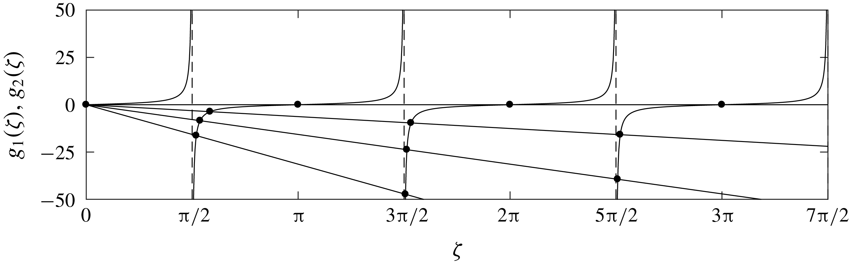
Graphical depiction of the intersections (circles) of
 $g_{1}(\unicode[STIX]{x1D701})=\tan \unicode[STIX]{x1D701}$
and
 $g_{2}(\unicode[STIX]{x1D701})=-{\mathcal{R}}\,\unicode[STIX]{x1D701}$
(where
 $g(\unicode[STIX]{x1D701})$
is defined in (5.6)) corresponding to the first three substrate (
 $n=1,2,3$
) roots
 $\unicode[STIX]{x1D706}=i\unicode[STIX]{x1D701}_{n}$
(circles) that satisfy
 $g(\unicode[STIX]{x1D701}_{n})=0$
for
 ${\mathcal{R}}=\{0,2,5,10\}$
. The line
 ${\mathcal{R}}=0$
is shown for reference, however physically
 ${\mathcal{R}}>0$
, with
 ${\mathcal{R}}=0$
corresponding to
 ${\mathcal{S}}\rightarrow \infty$
(approached when
 ${\mathcal{S}}\gg {\mathcal{B}}$
).

The roots
 $\unicode[STIX]{x1D701}_{n}$
are presented graphically in figure 2 as the intersections of the functions
 $g_{1}(\unicode[STIX]{x1D701})=\tan \unicode[STIX]{x1D701}$
and
 $g_{2}(\unicode[STIX]{x1D701})=-{\mathcal{R}}\,\unicode[STIX]{x1D701}$
. In the limit of small
 ${\mathcal{R}}\ll 1$
(respectively large
 ${\mathcal{R}}\gg 1$
), the roots
 $\unicode[STIX]{x1D701}_{n}$
asymptotically approach the zeros of
 $\cos \unicode[STIX]{x1D701}_{n}$
(respectively
 $\sin \unicode[STIX]{x1D701}_{n}$
). In the asymptotic limit
 $n\rightarrow \infty$
, the roots
 $\unicode[STIX]{x1D701}_{n}\rightarrow n\unicode[STIX]{x03C0}-\unicode[STIX]{x03C0}/2$
.
We now restrict attention to the roots
 $\unicode[STIX]{x1D706}_{+n}(0)$
,
 $n\geqslant 0$
, initialized to the upper half-plane (and for brevity drop the
 $+$
in the subscript of
 $\unicode[STIX]{x1D706}_{+n}(\unicode[STIX]{x1D6FD})$
), since the remaining roots are negatives by symmetry of (5.1). With the roots
 $\unicode[STIX]{x1D706}(\unicode[STIX]{x1D6FD})$
of (4.25) initialized to
 $\unicode[STIX]{x1D706}_{n}(0)=i\unicode[STIX]{x1D701}_{n}$
, we continuously vary
 $\unicode[STIX]{x1D6FD}\in [0,\infty )$
and track the roots
 $\unicode[STIX]{x1D706}_{n}(\unicode[STIX]{x1D6FD})$
as functions of
 $\unicode[STIX]{x1D6FD}$
. In our subsequent linear stability analysis, the
 $\unicode[STIX]{x1D706}_{0}(\unicode[STIX]{x1D6FD})$
root (initialized to
 $\unicode[STIX]{x1D706}_{0}(0)=0$
) will play a particularly important role. As a result, we will refer to
 $\unicode[STIX]{x1D706}_{0}(\unicode[STIX]{x1D6FD})$
as the film root, and (from now on) write
 $\unicode[STIX]{x1D706}_{f}(\unicode[STIX]{x1D6FD})$
. The phrase ‘film root’ is motivated by the fact that the corresponding complex frequency
 $\unicode[STIX]{x1D6FA}_{f}(\unicode[STIX]{x1D6FD})=\unicode[STIX]{x1D706}_{f}(\unicode[STIX]{x1D6FD})^{2}-\unicode[STIX]{x1D6FD}^{2}$
is analogous to the frequencies
 $\unicode[STIX]{x1D6FA}(\unicode[STIX]{x1D6FD})$
given by a free thin-film equation (see for instance appendix A). The remaining roots are initialized to
 $\unicode[STIX]{x1D706}_{n}(0)=i\unicode[STIX]{x1D701}_{n}$
for
 $n=1,2,\ldots$
.
As a technical point, we stress that the roots
 $\unicode[STIX]{x1D706}_{f}(\unicode[STIX]{x1D6FD})$
or
 $\unicode[STIX]{x1D706}_{n}(\unicode[STIX]{x1D6FD})$
are only (uniquely) identifiable by their initial values
 $i\unicode[STIX]{x1D701}_{n}$
within an interval
 $0\leqslant \unicode[STIX]{x1D6FD}\leqslant \unicode[STIX]{x1D6FD}_{coll}$
for which no collision has occurred. Once a collision occurs, i.e. two (or more) roots merge at a value
 $\unicode[STIX]{x1D6FD}=\unicode[STIX]{x1D6FD}_{coll}$
, it is generally not possible to identify uniquely two (or more) post-collision roots
 $\unicode[STIX]{x1D706}(\unicode[STIX]{x1D6FD})$
at values
 $\unicode[STIX]{x1D6FD}>\unicode[STIX]{x1D6FD}_{coll}$
with their initial values
 $i\unicode[STIX]{x1D701}_{n}$
.
As a final remark on the numerical computations, we follow a standard continuation approach: at each step, using the value
 $\unicode[STIX]{x1D706}(\unicode[STIX]{x1D6FD})$
as an initial guess, we use Newton’s method to compute
 $\unicode[STIX]{x1D706}(\unicode[STIX]{x1D6FD}+\unicode[STIX]{x0394}\unicode[STIX]{x1D6FD})$
, where
 $\unicode[STIX]{x0394}\unicode[STIX]{x1D6FD}$
is the increment (chosen adaptively to ensure convergence at each step). As a practical detail, to enable the method to find complex-valued solutions, we initialize the Newton algorithm with a value that does not lie strictly on either the real or complex axis by perturbing the initial guess via
 $\unicode[STIX]{x1D706}(\unicode[STIX]{x1D6FD})+\unicode[STIX]{x1D700}(1+i)$
, for
 $\unicode[STIX]{x1D700}\ll 1$
. This is to avoid having Newton iterates become trapped to the (invariant) real or complex axis.
5.2 Asymptotic behaviour of the roots for small
 $\unicode[STIX]{x1D6FD}$

The previous section demonstrates that the values
 $\unicode[STIX]{x1D706}_{n}(0)=i\unicode[STIX]{x1D701}_{n}$
are purely imaginary. Hence, at
 $\unicode[STIX]{x1D6FD}=0$
, the growth rates
 $\unicode[STIX]{x1D6FA}$
lie along the negative real axis:
 $\unicode[STIX]{x1D6FA}_{f}(0)=0$
(corresponding to the film root
 $\unicode[STIX]{x1D706}_{f}(0)=0$
), and
 $\unicode[STIX]{x1D6FA}_{n}(0)=-\unicode[STIX]{x1D701}_{n}^{2}<0$
(for the roots
 $\unicode[STIX]{x1D706}_{n}(0)=i\unicode[STIX]{x1D701}_{n}$
,
 $n\neq 0$
); see (4.12). The purpose of this section is to examine how the values
 $\unicode[STIX]{x1D6FA}_{n}(\unicode[STIX]{x1D6FD})$
and
 $\unicode[STIX]{x1D6FA}_{f}(\unicode[STIX]{x1D6FD})$
change for small values of
 $0\leqslant \unicode[STIX]{x1D6FD}\ll 1$
.
We first compute the small
 $\unicode[STIX]{x1D6FD}$
behaviour of the film root
 $\unicode[STIX]{x1D706}_{f}(\unicode[STIX]{x1D6FD})$
and corresponding growth rate
 $\unicode[STIX]{x1D6FA}_{f}(\unicode[STIX]{x1D6FD})$
. This can be done by expanding (4.25) in powers of
 $\unicode[STIX]{x1D706}$
(about
 $\unicode[STIX]{x1D706}_{f}(0)=0$
) to obtain
 $$\begin{eqnarray}\displaystyle f(\unicode[STIX]{x1D706},\unicode[STIX]{x1D6FD})=(a_{1}+a_{2})+(b_{1}+b_{2}-{\textstyle \frac{1}{3}}a_{1})\unicode[STIX]{x1D706}^{2}+O(\unicode[STIX]{x1D706}^{4}), & & \displaystyle\end{eqnarray}$$
where, recall,
 $a_{1},a_{2},b_{1},b_{2}$
depend on
 $\unicode[STIX]{x1D6FD}$
via (4.22). Truncating the expansion (5.7) at
 $O(\unicode[STIX]{x1D706}^{4})$
, and setting
 $f(\unicode[STIX]{x1D706},\unicode[STIX]{x1D6FD})$
to zero, yields an approximate solution for
 $\unicode[STIX]{x1D706}_{f}(\unicode[STIX]{x1D6FD})$
, valid at small
 $\unicode[STIX]{x1D6FD}$
 $$\begin{eqnarray}\unicode[STIX]{x1D706}_{f}(\unicode[STIX]{x1D6FD})\approx \pm \sqrt{\frac{a_{1}+a_{2}}{b_{1}+b_{2}-\frac{1}{3}a_{1}}}=\unicode[STIX]{x1D702}_{1}\unicode[STIX]{x1D6FD}-\unicode[STIX]{x1D702}_{3}\unicode[STIX]{x1D6FD}^{3}+\cdots \,.\end{eqnarray}$$
Here, the Taylor coefficients
 $\unicode[STIX]{x1D702}_{1}$
and
 $\unicode[STIX]{x1D702}_{3}$
are
 $$\begin{eqnarray}\unicode[STIX]{x1D702}_{1}=\sqrt{1+\frac{{\mathcal{C}}\,{\mathcal{B}}^{2}\,\bar{\unicode[STIX]{x1D6E9}}_{H}^{2}}{2\,{\mathcal{Q}}}},\quad \text{and}\quad \unicode[STIX]{x1D702}_{3}=\frac{1}{6}\left[{\mathcal{S}}\bar{\unicode[STIX]{x1D6E9}}_{H}\unicode[STIX]{x1D702}_{1}+\frac{{\mathcal{B}}^{3}}{{\mathcal{Q}}\,{\mathcal{S}}^{2}\,\unicode[STIX]{x1D702}_{1}}\right],\end{eqnarray}$$
respectively, where
 $\unicode[STIX]{x1D702}_{3}$
has been written compactly using the definition of
 $\unicode[STIX]{x1D702}_{1}$
. The above calculation shows that the double root at
 $\unicode[STIX]{x1D706}_{f}(0)=0$
splits immediately into two real non-zero roots given (approximately) by (5.8). As a convention, we use
 $\unicode[STIX]{x1D706}_{f}(\unicode[STIX]{x1D6FD})$
to denote the positive branch in (5.8). Via (4.12) we then have the small-wavenumber expansion of the corresponding growth rate
 $\unicode[STIX]{x1D6FA}_{f}(\unicode[STIX]{x1D6FD})$
, viz.,
 $$\begin{eqnarray}\displaystyle \unicode[STIX]{x1D6FA}_{f}(\unicode[STIX]{x1D6FD}) & = & \displaystyle (\unicode[STIX]{x1D702}_{1}^{2}-1)\,\unicode[STIX]{x1D6FD}^{2}-2\,\unicode[STIX]{x1D702}_{1}\,\unicode[STIX]{x1D702}_{3}\,\unicode[STIX]{x1D6FD}^{4}+O(\unicode[STIX]{x1D6FD}^{6})\nonumber\\ \displaystyle & {\approx} & \displaystyle \frac{{\mathcal{C}}\,{\mathcal{B}}^{2}\,\bar{\unicode[STIX]{x1D6E9}}_{H}^{2}}{2\,{\mathcal{Q}}}\unicode[STIX]{x1D6FD}^{2}-\left[\frac{{\mathcal{B}}^{3}}{3\,{\mathcal{S}}^{2}\,{\mathcal{Q}}}+{\mathcal{S}}\,\bar{\unicode[STIX]{x1D6E9}}_{H}\left(\frac{1}{3}+\frac{{\mathcal{C}}\,{\mathcal{B}}^{2}\,\bar{\unicode[STIX]{x1D6E9}}_{H}^{2}}{6\,{\mathcal{Q}}}\right)\right]\unicode[STIX]{x1D6FD}^{4}.\end{eqnarray}$$
Here, the first term inside the square brackets describes capillary stabilization, and the other terms including
 $\bar{\unicode[STIX]{x1D6E9}}_{H}$
pertain to thermocapillary effects. Notably, this expression predicts that thermocapillarity acts both to destabilize small wavenumbers and stabilize large ones, in contrast to the strict thermocapillary destabilization observed for thin substrates (see appendix A). In particular, equation (5.10) shows that the relative importance of thermocapillary stabilization will increase for large
 ${\mathcal{S}}$
(substrate thickness), large
 ${\mathcal{C}}$
(imposed temperature difference), or small
 ${\mathcal{Q}}$
(diffusive effects).
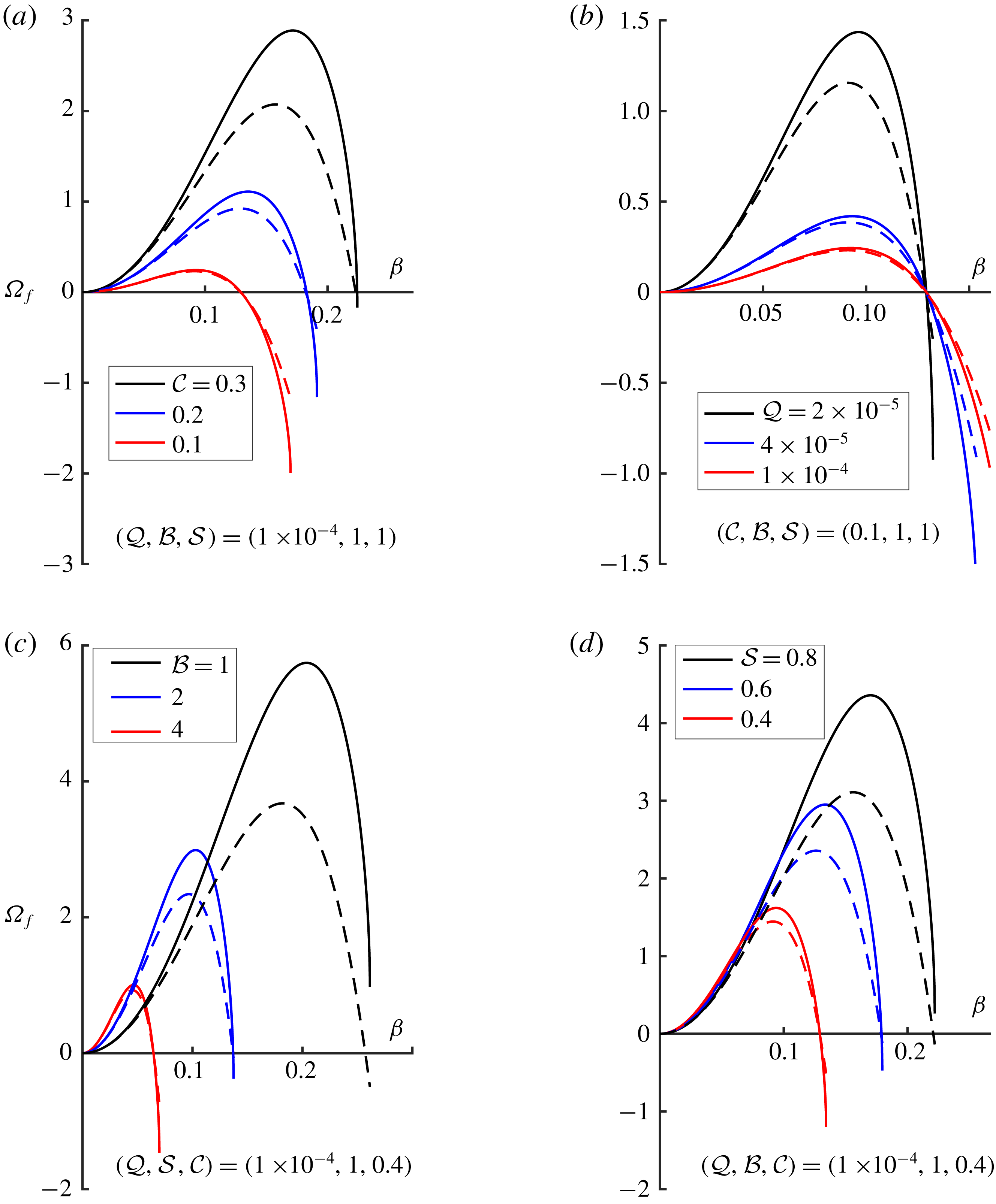
Comparison between the numerically calculated (solid lines, equation (4.25)) and approximated (dashed lines, equation (5.10)) film root growth rates
 $\unicode[STIX]{x1D6FA}_{f}(\unicode[STIX]{x1D6FD})$
for varying (a)
 ${\mathcal{C}}$
, (b)
 ${\mathcal{Q}}$
, (c)
 ${\mathcal{B}}$
and (d)
 ${\mathcal{S}}$
.

In figure 3, the small-
 $\unicode[STIX]{x1D6FD}$
approximation (5.10) for
 $\unicode[STIX]{x1D6FA}_{f}(\unicode[STIX]{x1D6FD})$
is compared to exact root branches calculated via numerical continuation. In each panel, one comparison is made to demonstrate a parameter set for which the agreement is qualitatively good; both the maximum growth rates and the cutoff wavenumbers are adequately predicted by (5.10). The surprisingly good prediction for the cutoff wavenumber is due to the original expansion in (5.7) being based on small
 $\unicode[STIX]{x1D706}$
: since
 $\unicode[STIX]{x1D706}^{2}=\unicode[STIX]{x1D6FA}+\unicode[STIX]{x1D6FD}^{2}$
, we expect the resulting approximation (5.10) to be good near the origin
 $\unicode[STIX]{x1D6FD}=\unicode[STIX]{x1D6FA}=0$
and at the cutoff where
 $\unicode[STIX]{x1D6FD}^{2}\ll 1$
still and
 $\unicode[STIX]{x1D6FA}=0$
. In the region between
 $\unicode[STIX]{x1D6FD}=0$
and the
 $O(1)$
cutoff values of the growth rate
 $\unicode[STIX]{x1D6FA}$
, the small-
 $\unicode[STIX]{x1D706}$
assumption made to obtain (5.7) is certainly violated. This is reflected in the poor agreement observed in this region between the asymptotic approximation (5.10) and the numerically calculated curves in figure 3.
Each branch in figure 3 is presented from
 $\unicode[STIX]{x1D6FD}=0$
to a critical value of
 $\unicode[STIX]{x1D6FD}_{coll}$
, beyond which the real film root ceases to exist (
 $\unicode[STIX]{x1D6FD}_{coll}$
will be defined more precisely below). Before focusing on these critical points in the next section, we note that several key physical behaviours can be inferred from figure 3. First, we see in panel (a) that larger imposed temperature differences (larger
 ${\mathcal{C}}$
) increase both the unstable band of wavenumbers and their associated growth rates. Panel (b) then shows that diffusive effects, as measured by
 ${\mathcal{Q}}$
, suppress the growth rates of instability without significantly changing the bandwidth of unstable wavenumbers. The loss of agreement in panel (c) occurs because, thinner films, via small values of
 ${\mathcal{B}}$
, promote the relative importance of the substrate thermal process.
Panel (d) shows the dependence on
 $\unicode[STIX]{x1D6FA}_{f}(\unicode[STIX]{x1D6FD})$
on the parameter
 ${\mathcal{S}}$
. We note that the increase in the growth rates with
 ${\mathcal{S}}$
shown in panel (d) results from having scaled time with respect to
 $d^{2}$
, see (3.2). The (approximately linear) increase of
 $\unicode[STIX]{x1D6FA}_{f}$
with
 ${\mathcal{S}}$
shown here in fact corresponds to a linear decrease in the dimensional growth rates – due primarily to the increased thermal resistance of thicker substrates.
5.3 The roots for
$n\neq 0$

To examine the roots
 $\unicode[STIX]{x1D706}_{n}(\unicode[STIX]{x1D6FD})$
and
 $\unicode[STIX]{x1D6FA}_{n}(\unicode[STIX]{x1D6FD})$
with
 $n\neq 0$
in the small-
 $\unicode[STIX]{x1D6FD}$
limit, we substitute the power series,
 $$\begin{eqnarray}\unicode[STIX]{x1D706}_{n}(\unicode[STIX]{x1D6FD})=i(\unicode[STIX]{x1D701}_{n}-\unicode[STIX]{x1D6FD}^{2}\unicode[STIX]{x1D70E}_{n})+O(\unicode[STIX]{x1D6FD}^{4}),\end{eqnarray}$$
into the dispersion relation with
 $\unicode[STIX]{x1D701}_{n}$
as given by (5.6) (see also figure 2) and unknown coefficients
 $\unicode[STIX]{x1D70E}_{n}$
(which will turn out to be real). Such an expansion in even powers of
 $\unicode[STIX]{x1D6FD}$
is justified by the symmetry relations (5.1) and by the fact that the values
 $\unicode[STIX]{x1D706}_{n}(\unicode[STIX]{x1D6FD})$
are simple near
 $\unicode[STIX]{x1D6FD}=0$
. Note that this is in contrast to the roots
 $\pm \unicode[STIX]{x1D706}_{f}(\unicode[STIX]{x1D6FD})$
that emerge from the double root
 $\unicode[STIX]{x1D706}_{f}(0)$
, which does not have an even power series at
 $\unicode[STIX]{x1D6FD}=0$
(double roots generally split via a square root dependence on the continuation parameter).
Expanding
 $f(\unicode[STIX]{x1D706}_{n}(\unicode[STIX]{x1D6FD}),\unicode[STIX]{x1D6FD})=0$
(see (4.25)) for small
 $\unicode[STIX]{x1D6FD}$
, and setting the
 $O(\unicode[STIX]{x1D6FD}^{2})$
term to zero yields
 $$\begin{eqnarray}\unicode[STIX]{x1D70E}_{n}=\frac{{\mathcal{C}}\,{\mathcal{B}}\,{\mathcal{S}}\,\bar{\unicode[STIX]{x1D6E9}}_{H}^{2}}{2\,{\mathcal{Q}}\,\unicode[STIX]{x1D701}_{n}\,({\mathcal{S}}+(1+{\mathcal{B}})^{2}\bar{\unicode[STIX]{x1D6E9}}_{H}\,\unicode[STIX]{x1D701}_{n}^{2})}.\end{eqnarray}$$
In this expression,
 $\tan \unicode[STIX]{x1D701}_{n}$
has been replaced with
 $-{\mathcal{R}}\,\unicode[STIX]{x1D701}_{n}$
per (5.6) (recall that
 ${\mathcal{R}}={\mathcal{S}}^{-1}(1+{\mathcal{B}})$
). Substituting the expressions (5.11)–(5.12) into (4.12) yields
 $$\begin{eqnarray}\unicode[STIX]{x1D6FA}_{n}(\unicode[STIX]{x1D6FD})=-\unicode[STIX]{x1D701}_{n}^{2}+\unicode[STIX]{x1D6FD}^{2}(2\,\unicode[STIX]{x1D701}_{n}\,\unicode[STIX]{x1D70E}_{n}-1)+O(\unicode[STIX]{x1D6FD}^{4}).\end{eqnarray}$$
At zero wavenumber, all these roots are real and negative:
 $\unicode[STIX]{x1D6FA}_{n}(0)=-\unicode[STIX]{x1D701}_{n}^{2}$
. As
 $\unicode[STIX]{x1D6FD}$
increases from zero, if
 $2\,\unicode[STIX]{x1D701}_{n}\,\unicode[STIX]{x1D70E}_{n}>1$
, then the roots (initially) move along the negative real axis in the complex plane towards the right-half plane (RHP; we will also use LHP to denote the left-half plane). Alternatively if
 $2\,\unicode[STIX]{x1D701}_{n}\,\unicode[STIX]{x1D70E}_{n}<1$
, then the roots move to the left along the negative real axis (see figure 4).
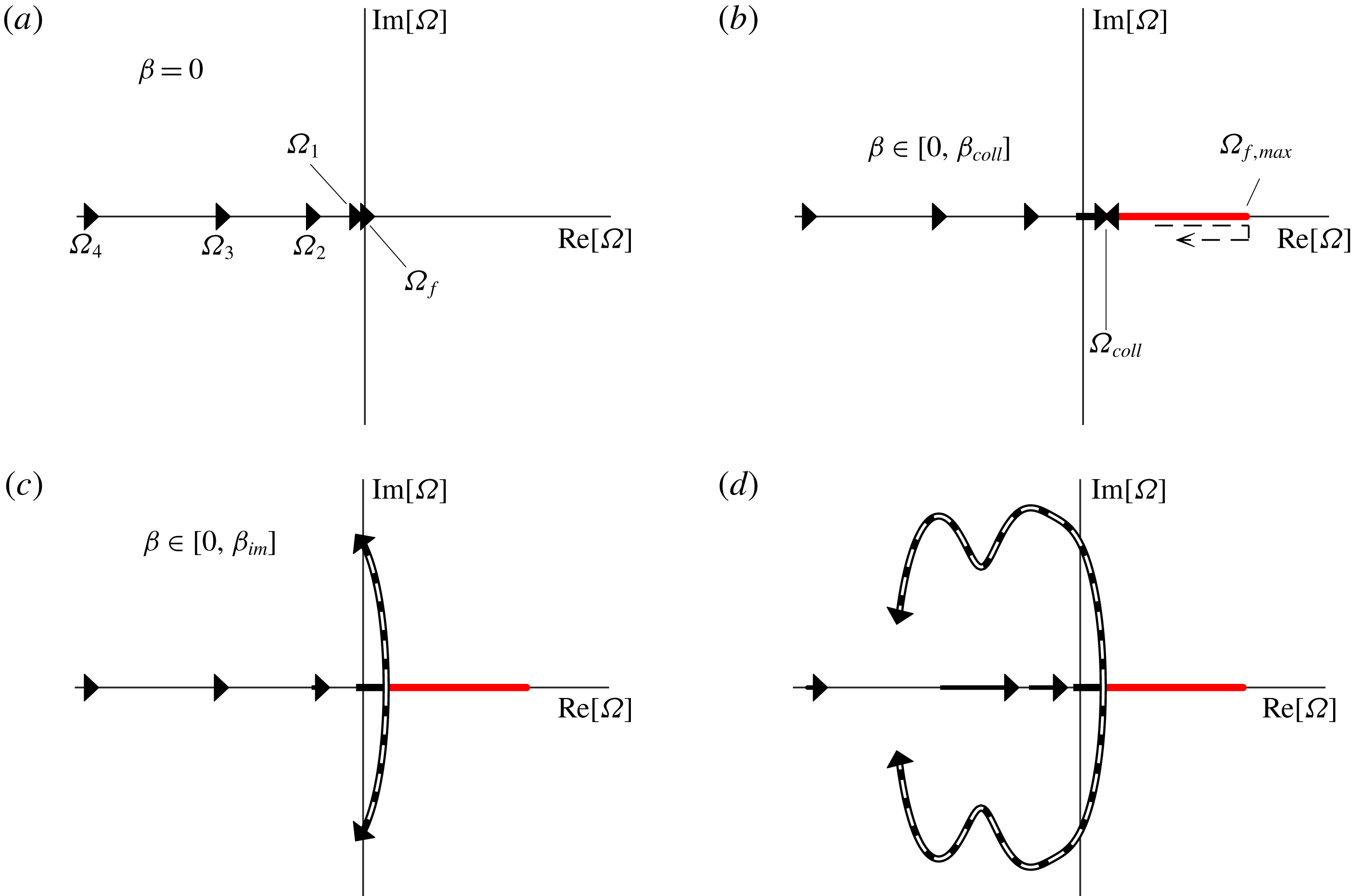
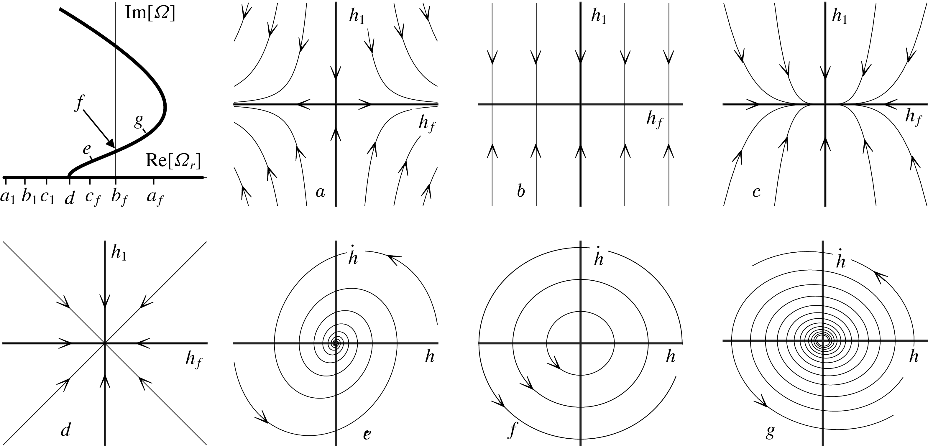
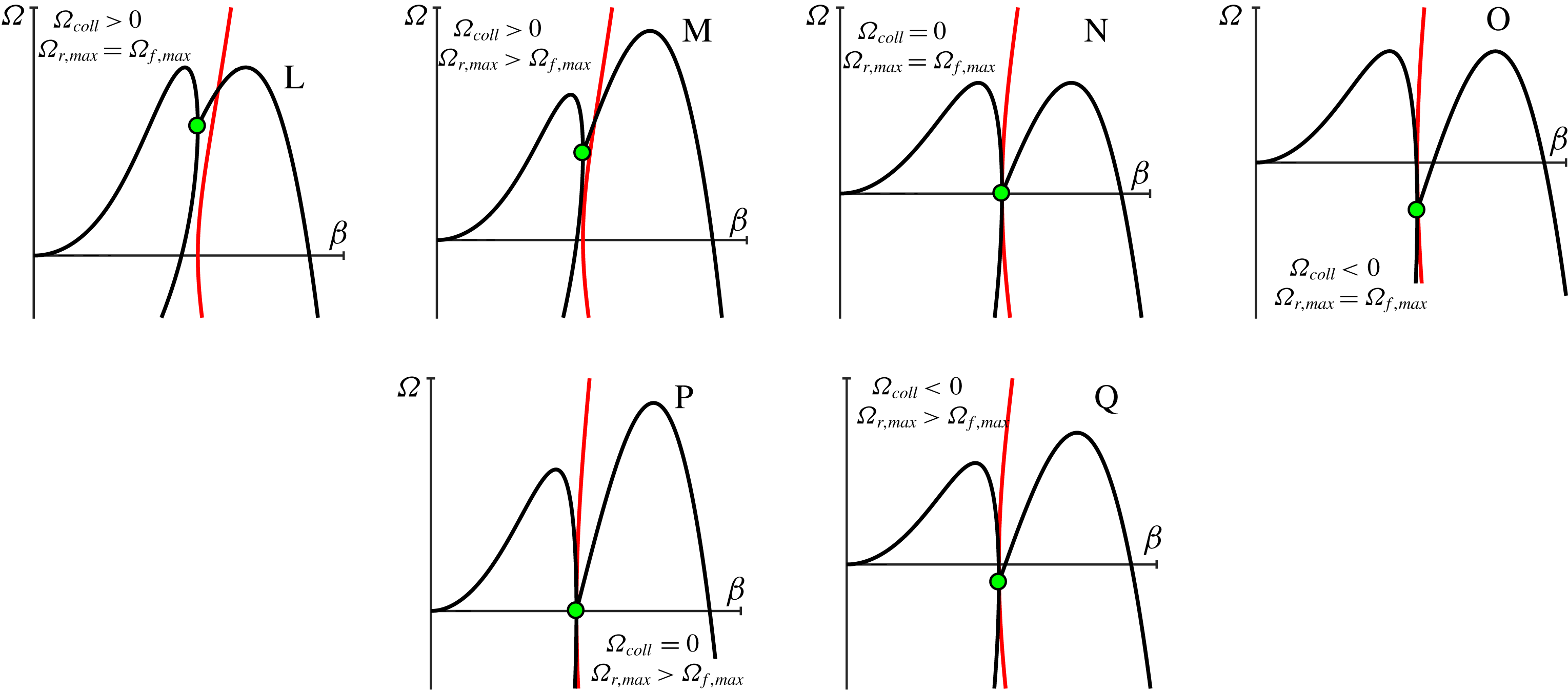
Shows the motion of the roots for a Type I oscillatory instability at increasing values of
 $\unicode[STIX]{x1D6FD}$
:
 $\unicode[STIX]{x1D6FD}=0$
(a),
 $\unicode[STIX]{x1D6FD}=\unicode[STIX]{x1D6FD}_{coll}$
(b),
 $\unicode[STIX]{x1D6FD}=\unicode[STIX]{x1D6FD}_{im}$
(c) and
 $\unicode[STIX]{x1D6FD}>\unicode[STIX]{x1D6FD}_{im}$
(d). The arrows denote the instantaneous location and direction of motion of the roots; the dark curves trace out the motion of the roots (with the white inset dashed line showing the motion after collisions); the red curve traces out the motion of the film root
 $\unicode[STIX]{x1D6FA}_{f}$
prior to collision.

We now remark that the product
 $\unicode[STIX]{x1D701}_{n}\,\unicode[STIX]{x1D70E}_{n}>0$
is (i) always positive, (ii) monotonically decreases with increasing values of
 $n$
(due to the fact that the values
 $\unicode[STIX]{x1D701}_{n}$
monotonically increase with
 $n$
), and (iii)
 $\lim _{n\rightarrow \infty }\unicode[STIX]{x1D701}_{n}\,\unicode[STIX]{x1D70E}_{n}\rightarrow 0$
. As a result, only a finite number of the values
 $\unicode[STIX]{x1D6FA}_{n}(\unicode[STIX]{x1D6FD})$
(closest to the origin) can have a positive
 $O(\unicode[STIX]{x1D6FD}^{2})$
coefficient, and hence initially move towards the unstable RHP. All other roots move (at small
 $\unicode[STIX]{x1D6FD}$
) farther into the LHP. Figure 4 demonstrates, via the continuation method, the motion of the roots
 $\{\unicode[STIX]{x1D6FA}_{f}(\unicode[STIX]{x1D6FD}),\unicode[STIX]{x1D6FA}_{n}(\unicode[STIX]{x1D6FD})\}$
, with varying
 $\unicode[STIX]{x1D6FD}$
. The plot shows the film root (
 $\unicode[STIX]{x1D6FA}_{f}(0)=0$
) and
 $\unicode[STIX]{x1D6FA}_{n}(0)=-\unicode[STIX]{x1D701}_{n}^{2}$
roots at
 $\unicode[STIX]{x1D6FD}=0$
. The arrows for the markers denote the numerically computed directions in which the roots move as
 $\unicode[STIX]{x1D6FD}>0$
increases. The arrows also coincide with the small-
 $\unicode[STIX]{x1D6FD}$
approximations (5.10) and (5.13). Note that the figure also demonstrates that the roots become complex only after a collision, and generally move to the left (becoming more stable) with increasing
 $\unicode[STIX]{x1D6FD}$
.
6 Oscillatory instability classification
In this section, we investigate how the frequencies
 $\unicode[STIX]{x1D6FA}_{f}(\unicode[STIX]{x1D6FD})$
and
 $\unicode[STIX]{x1D6FA}_{n}(\unicode[STIX]{x1D6FD})$
move in the complex plane (as functions of the continuation parameter
 $\unicode[STIX]{x1D6FD}$
), and lead to oscillating in time solutions of the linearized equations (4.13)–(4.18) with exponentially growing amplitudes. A value
 $\unicode[STIX]{x1D6FA}$
(that satisfies the dispersion relation) is oscillatory unstable if
 $\unicode[STIX]{x1D6FA}$
lies in the strict RHP, and does not lie along the real axis. That is,
 $\unicode[STIX]{x1D6FA}$
satisfies
 $$\begin{eqnarray}\displaystyle \text{(i)}\quad \text{Re}(\unicode[STIX]{x1D6FA})>0,\quad \text{(ii)}\quad \text{Im}(\unicode[STIX]{x1D6FA})\neq 0. & & \displaystyle\end{eqnarray}$$
Combined with the symmetry observations from the previous section (§ 5), conditions (6.1a,b
) place restrictions on how exactly a root
 $\unicode[STIX]{x1D6FA}(\unicode[STIX]{x1D6FD})$
can become oscillatory unstable as the wavenumber
 $\unicode[STIX]{x1D6FD}$
increases from
 $0$
.
First, condition (ii) in (6.1a,b
) requires that (as
 $\unicode[STIX]{x1D6FD}$
varies) two frequencies
 $\unicode[STIX]{x1D6FA}(\unicode[STIX]{x1D6FD})$
must collide at some value of
 $\unicode[STIX]{x1D6FD}$
– that is, there is a value of
 $\unicode[STIX]{x1D6FD}$
for which two of the frequencies
 $\{\unicode[STIX]{x1D6FA}_{f}(\unicode[STIX]{x1D6FD}),\unicode[STIX]{x1D6FA}_{n}(\unicode[STIX]{x1D6FD})\}$
are equal. This is because the complex frequencies
 $\{\unicode[STIX]{x1D6FA}_{f}(0),\unicode[STIX]{x1D6FA}_{n}(0)\}$
are simple (at
 $\unicode[STIX]{x1D6FD}=0$
), move continuously with
 $\unicode[STIX]{x1D6FD}$
and cannot leave the real axis as long as they remain simple (due to conjugate symmetry of
 $\unicode[STIX]{x1D6FA}(\unicode[STIX]{x1D6FD})$
, see (5.1)). Hence, a necessary condition for (ii) is a collision (double frequency) at some
 $\unicode[STIX]{x1D6FD}$
.
Second, the results from § 5 show that the frequencies
 $\{\unicode[STIX]{x1D6FA}_{f}(0),\unicode[STIX]{x1D6FA}_{n}(0)\}$
are on the non-positive real axis, and only a finite number of the largest roots initially move towards the RHP (as
 $\unicode[STIX]{x1D6FD}$
increases). Hence, the two largest roots
 $\unicode[STIX]{x1D6FA}_{f}(\unicode[STIX]{x1D6FD})$
(film root) and
 $\unicode[STIX]{x1D6FA}_{1}(\unicode[STIX]{x1D6FD})$
are the most likely candidates to collide and satisfy (6.1a,b
). In other words, oscillatory instabilities most likely arise from the motion and collisions of
 $\unicode[STIX]{x1D6FA}_{f}(\unicode[STIX]{x1D6FD})$
and
 $\unicode[STIX]{x1D6FA}_{1}(\unicode[STIX]{x1D6FD})$
.
Treating the continuation parameter
 $\unicode[STIX]{x1D6FD}$
as a bifurcation parameter (holding the parameters
 $({\mathcal{C}},{\mathcal{Q}},{\mathcal{B}},{\mathcal{S}})$
fixed), we now classify how exactly
 $\unicode[STIX]{x1D6FA}_{f}(\unicode[STIX]{x1D6FD})$
and
 $\unicode[STIX]{x1D6FA}_{1}(\unicode[STIX]{x1D6FD})$
collide (bifurcate) and satisfy (6.1a,b
) (lead to oscillatory instabilities). We define the (first) collision of
 $\{\unicode[STIX]{x1D6FA}_{f}(\unicode[STIX]{x1D6FD}),\unicode[STIX]{x1D6FA}_{1}(\unicode[STIX]{x1D6FD})\}$
to occur at the value
 $\unicode[STIX]{x1D6FD}_{coll}$
, and denote
 $$\begin{eqnarray}\displaystyle \unicode[STIX]{x1D6FA}_{coll}\equiv \lim _{\unicode[STIX]{x1D6FD}\rightarrow \unicode[STIX]{x1D6FD}_{coll}^{-}}\unicode[STIX]{x1D6FA}_{f}(\unicode[STIX]{x1D6FD})=\lim _{\unicode[STIX]{x1D6FD}\rightarrow \unicode[STIX]{x1D6FD}_{coll}^{-}}\unicode[STIX]{x1D6FA}_{1}(\unicode[STIX]{x1D6FD}). & & \displaystyle\end{eqnarray}$$
Note that the values
 $(\unicode[STIX]{x1D6FD}_{coll},\unicode[STIX]{x1D6FA}_{coll})$
are readily identifiable: in addition to the dispersion relation
 $\unicode[STIX]{x1D6FA}_{coll}=\unicode[STIX]{x1D706}_{coll}^{2}-\unicode[STIX]{x1D6FD}_{coll}^{2}$
, with
 $f(\unicode[STIX]{x1D706}_{coll},\unicode[STIX]{x1D6FD}_{coll})=0$
, the values
 $(\unicode[STIX]{x1D6FD}_{coll},\unicode[STIX]{x1D6FA}_{coll})$
satisfy the condition of a double root required by the implicit function theorem,
 $\unicode[STIX]{x2202}_{\unicode[STIX]{x1D706}}f(\unicode[STIX]{x1D706}_{coll},\unicode[STIX]{x1D6FD}_{coll})=0$
. For values of
 $\unicode[STIX]{x1D6FD}\in [0,\unicode[STIX]{x1D6FD}_{coll}]$
, the frequencies
 $\unicode[STIX]{x1D6FA}_{f}(\unicode[STIX]{x1D6FD}),\unicode[STIX]{x1D6FA}_{1}(\unicode[STIX]{x1D6FD})\in \mathbb{R}$
; however, for
 $\unicode[STIX]{x1D6FD}>\unicode[STIX]{x1D6FD}_{coll}$
(after the collision), the roots appear as complex conjugate pairs that we denote as
 $\unicode[STIX]{x1D6FA}_{f,1}(\unicode[STIX]{x1D6FD})=\unicode[STIX]{x1D6FA}_{r}(\unicode[STIX]{x1D6FD})+i\unicode[STIX]{x1D6FA}_{i}(\unicode[STIX]{x1D6FD})$
and
 $\unicode[STIX]{x1D6FA}_{f,1}^{\ast }(\unicode[STIX]{x1D6FD})$
, with
 $\unicode[STIX]{x1D6FA}_{r}(\unicode[STIX]{x1D6FD}),\unicode[STIX]{x1D6FA}_{i}(\unicode[STIX]{x1D6FD})\in \mathbb{R}$
. We further denote
 $\unicode[STIX]{x1D6FD}_{im}>\unicode[STIX]{x1D6FD}_{coll}$
(if it exists) as the first value at which the frequency
 $\unicode[STIX]{x1D6FA}_{f,1}(\unicode[STIX]{x1D6FD})$
crosses the imaginary axis, i.e.
 $\unicode[STIX]{x1D6FA}_{r}(\unicode[STIX]{x1D6FD}_{im})=0$
. Summarizing the notation, we have
 $$\begin{eqnarray}\left.\begin{array}{@{}c@{}}\text{(Pre-collision)}\;0\leqslant \unicode[STIX]{x1D6FD}<\unicode[STIX]{x1D6FD}_{coll}\;\Longrightarrow \;\unicode[STIX]{x1D6FA}_{1}(\unicode[STIX]{x1D6FD})<\unicode[STIX]{x1D6FA}_{f}(\unicode[STIX]{x1D6FD}),\text{ and }\unicode[STIX]{x1D6FA}_{f}(\unicode[STIX]{x1D6FD}),\unicode[STIX]{x1D6FA}_{1}(\unicode[STIX]{x1D6FD})\in \mathbb{R},\\ \text{(At collision)}\;\unicode[STIX]{x1D6FD}=\unicode[STIX]{x1D6FD}_{coll}\;\Longrightarrow \;\unicode[STIX]{x1D6FA}_{coll}\equiv \unicode[STIX]{x1D6FA}_{coll}(\unicode[STIX]{x1D6FD})=\unicode[STIX]{x1D6FA}_{f}(\unicode[STIX]{x1D6FD}),\text{ and }\unicode[STIX]{x1D6FA}_{coll}\in \mathbb{R},\\ \text{(Post-collision)}\;\unicode[STIX]{x1D6FD}>\unicode[STIX]{x1D6FD}_{coll}\;\Longrightarrow \;\unicode[STIX]{x1D6FA}_{f,1}(\unicode[STIX]{x1D6FD})=\unicode[STIX]{x1D6FA}_{r}(\unicode[STIX]{x1D6FD})+i\unicode[STIX]{x1D6FA}_{i}(\unicode[STIX]{x1D6FD}),\text{and }\unicode[STIX]{x1D6FA}_{f,1}^{\ast }(\unicode[STIX]{x1D6FD}),\\ \text{(Imag. axis)}\;\unicode[STIX]{x1D6FD}=\unicode[STIX]{x1D6FD}_{im}\;\Longrightarrow \;\unicode[STIX]{x1D6FA}_{r}(\unicode[STIX]{x1D6FD}_{im})=0,\text{ (}\unicode[STIX]{x1D6FD}_{im}\geqslant \unicode[STIX]{x1D6FD}_{coll}\text{ may not exist)}.\end{array}\right\}\end{eqnarray}$$
We now identify two characteristic ways for the roots
 $\unicode[STIX]{x1D6FA}_{f}(\unicode[STIX]{x1D6FD}),\unicode[STIX]{x1D6FA}_{1}(\unicode[STIX]{x1D6FD})$
to satisfy conditions (6.1a,b
) and give rise to oscillatory instabilities.
Type I oscillatory instabilities. Top-left panel (boxed region in figure 4 shows the motion of
 $\unicode[STIX]{x1D6FA}_{1}(\unicode[STIX]{x1D6FD})$
,
 $\unicode[STIX]{x1D6FA}_{f}(\unicode[STIX]{x1D6FD})$
and
 $\unicode[STIX]{x1D6FA}_{f,1}(\unicode[STIX]{x1D6FD})$
(in bold) as
 $\unicode[STIX]{x1D6FD}\geqslant 0$
varies to satisfy conditions (6.1a,b
). Subfigures (a–g) Are the linear phase plane for the time evolution of a perturbed solution from (4.1), made to the film height. Perturbations are excited at frequencies
 $\unicode[STIX]{x1D6FA}_{1}(\unicode[STIX]{x1D6FD}),\unicode[STIX]{x1D6FA}_{f}(\unicode[STIX]{x1D6FD})$
or
 $\unicode[STIX]{x1D6FA}_{f,1}(\unicode[STIX]{x1D6FD})$
that coincide with locations (a–g) for different
 $\unicode[STIX]{x1D6FD}$
values in the top-left panel.

Type I:
 $\unicode[STIX]{x1D6FA}_{coll}>0$
. The top-left panel of figures 5 highlights how the frequencies
 $\unicode[STIX]{x1D6FA}_{f}(\unicode[STIX]{x1D6FD}),\unicode[STIX]{x1D6FA}_{1}(\unicode[STIX]{x1D6FD})$
move from locations
 $a$
–
 $c$
at wavenumbers
 $\unicode[STIX]{x1D6FD}<\unicode[STIX]{x1D6FD}_{coll}$
; collide at location
 $d$
(
 $\unicode[STIX]{x1D6FD}=\unicode[STIX]{x1D6FD}_{coll}$
with
 $\unicode[STIX]{x1D6FA}_{coll}>0$
); are unstable and satisfy (6.1a,b
) at any point
 $e$
between
 $d$
and
 $f$
; cross over into the LHP at
 $f$
; and are stable at points
 $g$
in the LHP. The behaviour of the perturbations (4.1) qualitatively changes at different wavenumbers
 $\unicode[STIX]{x1D6FD}$
through a series of bifurcations. To provide a visual characterization of the linearized dynamics of the perturbations (4.1) at different points
 $a$
–
 $g$
, we plot the phase plane trajectories in the eigenmodes with frequencies
 $\unicode[STIX]{x1D6FA}_{f}(\unicode[STIX]{x1D6FD}),\unicode[STIX]{x1D6FA}_{1}(\unicode[STIX]{x1D6FD})$
(when
 $0\leqslant \unicode[STIX]{x1D6FD}\leqslant \unicode[STIX]{x1D6FD}_{coll}$
) or frequencies
 $\unicode[STIX]{x1D6FA}_{f,1}(\unicode[STIX]{x1D6FD}),\unicode[STIX]{x1D6FA}_{f,1}^{\ast }(\unicode[STIX]{x1D6FD})$
(for
 $\unicode[STIX]{x1D6FD}>\unicode[STIX]{x1D6FD}_{coll}$
). For wavenumbers
 $\unicode[STIX]{x1D6FD}\leqslant \unicode[STIX]{x1D6FD}_{coll}$
, a perturbation in
 $H(X,T)$
with amplitude
 $\unicode[STIX]{x1D6FF}{\hat{H}}_{f}$
in frequency
 $\unicode[STIX]{x1D6FA}_{f}(\unicode[STIX]{x1D6FD})$
, and amplitude
 $\unicode[STIX]{x1D6FF}{\hat{H}}_{1}$
in frequency
 $\unicode[STIX]{x1D6FA}_{1}(\unicode[STIX]{x1D6FD})$
, evolves as
 $$\begin{eqnarray}H(X,T)={\mathcal{B}}+\unicode[STIX]{x1D6FF}\;\cos (\unicode[STIX]{x1D6FD}X)\left[\underbrace{{\hat{H}}_{f}\exp (\unicode[STIX]{x1D6FA}_{f}(\unicode[STIX]{x1D6FD})T)}_{h_{f}(T)}+\underbrace{{\hat{H}}_{1}\exp (\unicode[STIX]{x1D6FA}_{1}(\unicode[STIX]{x1D6FD})T)}_{h_{1}(T)}\right]+O(\unicode[STIX]{x1D6FF}^{2}).\end{eqnarray}$$
Figure 5(a–d) plots the phase plane dynamics in the
 $h_{1}(T)$
–
 $h_{f}(T)$
plane. For wavenumbers
 $\unicode[STIX]{x1D6FD}>\unicode[STIX]{x1D6FD}_{coll}$
, the frequencies are complex
 $\unicode[STIX]{x1D6FA}_{f,1}(\unicode[STIX]{x1D6FD})$
,
 $\unicode[STIX]{x1D6FA}_{f,1}(\unicode[STIX]{x1D6FD})^{\ast }$
and we write the perturbation as
 $$\begin{eqnarray}\displaystyle H(X,T) & = & \displaystyle {\mathcal{B}}+\unicode[STIX]{x1D6FF}\;\cos (\unicode[STIX]{x1D6FD}X)\left[\underbrace{{\hat{H}}_{R}\text{Re}[\exp (\unicode[STIX]{x1D6FA}_{f,1}(\unicode[STIX]{x1D6FD})T)]}_{h(T)}+\underbrace{{\hat{H}}_{I}\text{Re}[\unicode[STIX]{x1D6FA}_{f,1}(\unicode[STIX]{x1D6FD})\exp (\unicode[STIX]{x1D6FA}_{f,1}(\unicode[STIX]{x1D6FD})T)]}_{\text{d}h(T)}\right]\nonumber\\ \displaystyle & & \displaystyle +\,O(\unicode[STIX]{x1D6FF}^{2}),\end{eqnarray}$$
where
 ${\hat{H}}_{R}$
and
 ${\hat{H}}_{I}$
are the two amplitudes of the perturbation. The panels
 $e$
–
 $g$
in figure 5 plot the phase plane trajectories in the
 $h(T)$
–
 $\text{d}h(T)$
plane. Here we use the short-form notation
 $\text{d}h(T)$
for the second linearly independent term in (6.5) since it is proportional to
 $\text{d}h/\text{d}t$
. The panels show the qualitatively different phase plane behaviour, and emergence of oscillatory instabilities, as the bifurcation parameter
 $\unicode[STIX]{x1D6FD}$
varies. The boundary in the parameter space
 $({\mathcal{C}},{\mathcal{Q}},{\mathcal{B}},{\mathcal{S}})$
, for Type I behaviour to occur, must satisfy (as a necessary condition)
 $\unicode[STIX]{x1D6FA}_{coll}=0$
.
The temperature eigenfunction profiles defined by (4.28)–(4.29) at two values of
 $\unicode[STIX]{x1D6FD}$
for a Type I oscillatory instability. (a)
 $\unicode[STIX]{x1D6FD}<\unicode[STIX]{x1D6FD}_{coll}$
prior to collision. For this value of
 $\unicode[STIX]{x1D6FD}=0.39$
both eigenfunctions are real and unstable. (b)
 $\unicode[STIX]{x1D6FD}=0.42$
and
 $\unicode[STIX]{x1D6FD}_{coll}<0.42<\unicode[STIX]{x1D6FD}_{im}$
; one complex eigenfunction is oscillatory instability. The eigenfunctions are plotted for parameter values
 $({\mathcal{Q}},{\mathcal{C}},{\mathcal{B}},{\mathcal{S}})=(1\times 10^{-4},1,2,2)$
.

Figure 6 plots the spatial profiles for the temperature eigenfunctions
 $\{\hat{\unicode[STIX]{x1D6E9}}({\tilde{Y}}),\hat{\mathit{\{}}(Y)\}$
defined by (4.28)–(4.29) for two values of
 $\unicode[STIX]{x1D6FD}$
in a Type I oscillatory instability. The figure highlights that for
 $\unicode[STIX]{x1D6FD}=0.39<\unicode[STIX]{x1D6FD}_{im}$
, the values of
 $\unicode[STIX]{x1D706}_{f}(\unicode[STIX]{x1D6FD})$
and
 $\unicode[STIX]{x1D706}_{1}(\unicode[STIX]{x1D6FD})$
(which play the role of wavenumbers) are both real, yielding two real eigenfunctions (left panel). For
 $\unicode[STIX]{x1D6FD}_{coll}<0.42<\unicode[STIX]{x1D6FD}_{im}$
, the continuation of the values of
 $\unicode[STIX]{x1D706}_{f}(\unicode[STIX]{x1D6FD})$
and
 $\unicode[STIX]{x1D706}_{1}(\unicode[STIX]{x1D6FD})$
collide and become complex, giving rise to one complex eigenfunction (right panel). The real and imaginary parts of the complex eigenfunction may oscillate in space, and correspond to the temperature profile of an oscillatory instability.
Type II:
 $\unicode[STIX]{x1D6FA}_{coll}\leqslant 0$
and
 $\unicode[STIX]{x1D6FA}_{r}(\unicode[STIX]{x1D6FD})>0$
for some
 $\unicode[STIX]{x1D6FD}>\unicode[STIX]{x1D6FD}_{coll}$
. Figure 7 highlights (via arrows) the motion of the roots
 $\unicode[STIX]{x1D6FA}_{f}(\unicode[STIX]{x1D6FD})$
(red),
 $\unicode[STIX]{x1D6FA}_{1}(\unicode[STIX]{x1D6FD})$
(black) and post collision roots
 $\unicode[STIX]{x1D6FA}_{f,1}(\unicode[STIX]{x1D6FD})$
(black with white dashed line) with varying
 $\unicode[STIX]{x1D6FD}$
. The top-left panel in figure 8 shows again the motion of the frequencies
 $\unicode[STIX]{x1D6FA}_{f}(\unicode[STIX]{x1D6FD})$
,
 $\unicode[STIX]{x1D6FA}_{1}(\unicode[STIX]{x1D6FD})$
, and
 $\unicode[STIX]{x1D6FA}_{f,1}(\unicode[STIX]{x1D6FD})$
. The frequencies
 $\unicode[STIX]{x1D6FA}_{f}(\unicode[STIX]{x1D6FD})$
,
 $\unicode[STIX]{x1D6FA}_{1}(\unicode[STIX]{x1D6FD})$
move from locations
 $a$
–
 $c$
and collide at
 $d$
with
 $\unicode[STIX]{x1D6FA}_{coll}\leqslant 0$
. The values
 $\unicode[STIX]{x1D6FA}_{f,1}(\unicode[STIX]{x1D6FD})$
are complex at location
 $e$
, and then move into the right-half plane
 $\unicode[STIX]{x1D6FA}_{r}(\unicode[STIX]{x1D6FD})\geqslant 0$
at
 $f$
–
 $g$
; thereby satisfying conditions (6.1a,b
). The figures also show the phase plane trajectories for perturbations to the film height (in a fashion completely analogous to figure 5) given by (6.4)–(6.5). The boundary in the parameter space
 $({\mathcal{C}},{\mathcal{Q}},{\mathcal{B}},{\mathcal{S}})$
, for Type II behaviour, requires (as a necessary condition) that
 $\max _{\unicode[STIX]{x1D6FD}\geqslant \unicode[STIX]{x1D6FD}_{coll}}\unicode[STIX]{x1D6FA}_{r}(\unicode[STIX]{x1D6FD})=0$
.
The motion of the roots for a Type II oscillatory instability at increasing values of
 $\unicode[STIX]{x1D6FD}$
:
 $\unicode[STIX]{x1D6FD}=\unicode[STIX]{x1D6FD}_{im}$
(a),
 $\unicode[STIX]{x1D6FD}>\unicode[STIX]{x1D6FD}_{im}$
(b). The arrows denote the instantaneous location and direction of motion of the roots; the dark curves trace out the motion of the roots (with the white inset dashed line showing the motion after collisions); the red curve traces out the motion of the film root
 $\unicode[STIX]{x1D6FA}_{f}$
prior to collision. The collision occurs on the negative real axis (
 $\unicode[STIX]{x1D6FA}_{coll}<0$
) and before entering into the RHP.

Type II oscillatory instabilities. Top-left panel (boxed region in left panel of figure 7) shows the motion of
 $\unicode[STIX]{x1D6FA}_{1}(\unicode[STIX]{x1D6FD})$
,
 $\unicode[STIX]{x1D6FA}_{f}(\unicode[STIX]{x1D6FD})$
and
 $\unicode[STIX]{x1D6FA}_{f,1}(\unicode[STIX]{x1D6FD})$
(in bold) as
 $\unicode[STIX]{x1D6FD}\geqslant 0$
varies to satisfy conditions (6.1a,b
). Subfigures (a–g) Are the linear phase plane portraits for the time evolution of a perturbation made to the film height excited at frequencies
 $\unicode[STIX]{x1D6FA}_{1}(\unicode[STIX]{x1D6FD}),\unicode[STIX]{x1D6FA}_{f}(\unicode[STIX]{x1D6FD})$
or
 $\unicode[STIX]{x1D6FA}_{f,1}(\unicode[STIX]{x1D6FD})$
and different
 $\unicode[STIX]{x1D6FD}$
values.

Having criteria for the boundaries in the parameter space
 $({\mathcal{C}},{\mathcal{Q}},{\mathcal{B}},{\mathcal{S}})$
of Types I or II oscillatory instabilities will become useful in the following section. Specifically, we will use these conditions to help plot phase diagrams and identify model parameters and experimental conditions that may yield oscillatory instabilities.
The underlying distinction between Types I and II instabilities occurs from viewing
 $\unicode[STIX]{x1D6FD}$
as a bifurcation parameter. Each root
 $\unicode[STIX]{x1D6FA}$
for any value of
 $\unicode[STIX]{x1D6FD}$
is associated with a linear dynamical system for the variables in (4.1). Type I oscillatory instabilities occur from one bifurcation when the roots collide at
 $\unicode[STIX]{x1D6FD}=\unicode[STIX]{x1D6FD}_{coll}$
. Meanwhile, Type II oscillatory instabilities occur through two bifurcations: the first at
 $\unicode[STIX]{x1D6FD}=\unicode[STIX]{x1D6FD}_{coll}$
when the roots collide, and the second at the value
 $\unicode[STIX]{x1D6FD}=\unicode[STIX]{x1D6FD}_{im}$
, when the roots enter into the RHP (e.g. see Strogatz (Reference Strogatz2015), chapter 8). Categorizing oscillatory instabilities as Type I or Type II through different bifurcations provides criteria that we will use in § 7 to systematically determine which parameter values
 $({\mathcal{C}},{\mathcal{Q}},{\mathcal{B}},{\mathcal{S}})$
give rise to oscillatory instabilities. Type I and Type II instabilities are physically distinguishable through their bands of unstable wavenumbers: Type I does not contain a band of wavenumbers with values
 $\unicode[STIX]{x1D6FD}<\unicode[STIX]{x1D6FD}_{coll}$
where
 $\unicode[STIX]{x1D6FA}_{f}(\unicode[STIX]{x1D6FD})$
is stable (figure 5 at points (
 $a$
–
 $d$
) are unstable); in contrast, Type II does contain an interval of wavenumbers with values
 $\unicode[STIX]{x1D6FD}<\unicode[STIX]{x1D6FD}_{coll}$
where
 $\unicode[STIX]{x1D6FA}_{f}(\unicode[STIX]{x1D6FD})$
is stable (figure 8 at points
 $c$
and
 $d$
are stable).
In addition to classifying Types I and II oscillatory instabilities, we further distinguish whether a set of parameters
 $({\mathcal{C}},{\mathcal{Q}},{\mathcal{B}},{\mathcal{S}})$
gives rise to dominant oscillatory instabilities. A set of parameters
 $({\mathcal{C}},{\mathcal{Q}},{\mathcal{B}},{\mathcal{S}})$
is said to be dominant oscillatory unstable if there is a
 $\unicode[STIX]{x1D6FD}_{c,max}$
and
 $\unicode[STIX]{x1D6FA}_{c,max}=\unicode[STIX]{x1D6FA}(\unicode[STIX]{x1D6FD}_{c,max})$
satisfying the dispersion relation (4.24) that is oscillatory unstable, and has the largest growth rate
 $\text{Re}(\unicode[STIX]{x1D6FA}_{c,max})\geqslant \text{Re}(\unicode[STIX]{x1D6FA}(\unicode[STIX]{x1D6FD}))$
for all
 $\unicode[STIX]{x1D6FD}$
,
 $\unicode[STIX]{x1D6FA}(\unicode[STIX]{x1D6FD})$
(satisfying the dispersion relation (4.24)). Dominant oscillatory unstable parameter values are physically significant because they represent experimental situations where the most unstable perturbation to the linearized system (4.1) is oscillatory unstable (and hence the most likely to be observed).
In the numerical continuation of the roots
 $\{\unicode[STIX]{x1D6FA}_{f}(\unicode[STIX]{x1D6FD}),\unicode[STIX]{x1D6FA}_{n}(\unicode[STIX]{x1D6FD})\}$
, we have always observed that oscillatory instabilities arise as Type I or Type II, as described in this section. It may be possible that oscillatory instabilities occur from the collision of other roots (for instance, a collision including
 $\unicode[STIX]{x1D6FA}_{2}(\unicode[STIX]{x1D6FD})$
); however, we did not observe this in any of our investigations. If the only possible mechanism to obtain oscillatory instabilities is through Type I or Type II, and the largest growth rate
 $\unicode[STIX]{x1D6FA}_{c,max}$
occurs at a value
 $\unicode[STIX]{x1D6FA}_{f}(\unicode[STIX]{x1D6FD})$
(which we also numerically observe to be the case in our studies), then we may simplify the condition for dominant oscillatory instabilities to growth rates computed in terms of
 $\unicode[STIX]{x1D6FA}_{f}(\unicode[STIX]{x1D6FD})$
and
 $\unicode[STIX]{x1D6FA}_{f,1}(\unicode[STIX]{x1D6FD})$
by defining
 $$\begin{eqnarray}\unicode[STIX]{x1D6FA}_{f,max}\equiv \max _{0\leqslant \unicode[STIX]{x1D6FD}\leqslant \unicode[STIX]{x1D6FD}_{coll}}\unicode[STIX]{x1D6FA}_{f}(\unicode[STIX]{x1D6FD}),\quad \unicode[STIX]{x1D6FA}_{r,max}\equiv \max _{\unicode[STIX]{x1D6FD}\geqslant \unicode[STIX]{x1D6FD}_{coll}}\unicode[STIX]{x1D6FA}_{r}(\unicode[STIX]{x1D6FD}).\end{eqnarray}$$
The condition for dominant oscillatory instabilities is then
 $$\begin{eqnarray}\text{(Dominant oscillatory instabilities)}\quad \unicode[STIX]{x1D6FA}_{f,max}\leqslant \unicode[STIX]{x1D6FA}_{r,max}.\end{eqnarray}$$
To characterize oscillatory instabilities, we will also make use of the most unstable wavenumber,
 $\unicode[STIX]{x1D6FD}_{max}$
defined as
 $$\begin{eqnarray}\displaystyle \unicode[STIX]{x1D6FA}_{r,max}=\unicode[STIX]{x1D6FA}_{r}(\unicode[STIX]{x1D6FD}_{max}), & & \displaystyle\end{eqnarray}$$
or alternatively written as the argument of the maximum
 $\unicode[STIX]{x1D6FD}_{max}=\text{argmax}_{\unicode[STIX]{x1D6FD}\geqslant \unicode[STIX]{x1D6FD}_{coll}}\unicode[STIX]{x1D6FA}_{r}(\unicode[STIX]{x1D6FD})$
. We will also denote the imaginary frequency of the most unstable wavenumber as
 $\unicode[STIX]{x1D6FA}_{i,max}=\unicode[STIX]{x1D6FA}_{i}(\unicode[STIX]{x1D6FD}_{max})$
.
In practice, the maximization
 $\max _{\unicode[STIX]{x1D6FD}\geqslant \unicode[STIX]{x1D6FD}_{coll}}\unicode[STIX]{x1D6FA}_{r}(\unicode[STIX]{x1D6FD})$
in condition (6.7) implies that we maximize the real value of the root
 $\unicode[STIX]{x1D6FA}_{f,1}(\unicode[STIX]{x1D6FD})$
over a suitably large range of
 $\unicode[STIX]{x1D6FD}$
values (by taking
 $\unicode[STIX]{x1D6FD}$
large enough
 $\unicode[STIX]{x1D6FA}_{r}(\unicode[STIX]{x1D6FD})$
will eventually become negative). Replacing the inequality
 $({\leqslant})$
in (6.7) with an equality
 $(=)$
then provides a condition for the boundary of the dominant oscillatory instability region.
7 Emergence of oscillatory instabilities
The purpose of this section is to explore the model parameter space
 $({\mathcal{C}},{\mathcal{Q}},{\mathcal{B}},{\mathcal{S}})$
and characterize which parameter regions give rise to oscillatory instabilities. This will provide a guide for experimental scenarios in which one may likely see oscillatory instabilities. To compute these regions we use the formulas for the boundaries of the parameter regions, satisfied by Type I and Type II instabilities, developed in § 6. As a general guide, we also introduce a heuristic value
 $$\begin{eqnarray}\unicode[STIX]{x2202}_{\unicode[STIX]{x1D6FD}}\unicode[STIX]{x1D6FA}_{coll}\equiv \lim _{\unicode[STIX]{x1D6FD}\rightarrow \unicode[STIX]{x1D6FD}_{coll}^{+}}\frac{\text{d}}{\text{d}\unicode[STIX]{x1D6FD}}\unicode[STIX]{x1D6FA}_{r}(\unicode[STIX]{x1D6FD}),\end{eqnarray}$$
as the rate of change of the real value of the roots
 $\unicode[STIX]{x1D6FA}_{f,1}(\unicode[STIX]{x1D6FD})=\unicode[STIX]{x1D6FA}_{r}(\unicode[STIX]{x1D6FD})+i\unicode[STIX]{x1D6FA}_{i}(\unicode[STIX]{x1D6FD})$
immediately after the collision
 $\unicode[STIX]{x1D6FD}\rightarrow \unicode[STIX]{x1D6FD}_{coll}^{+}$
. A positive value
 $\unicode[STIX]{x2202}_{\unicode[STIX]{x1D6FD}}\unicode[STIX]{x1D6FA}_{r}>0$
(respectively
 ${<}$
) implies the roots
 $\unicode[STIX]{x1D6FA}_{f,1}(\unicode[STIX]{x1D6FD})$
move towards the right (respectively left) in the complex plane as
 $\unicode[STIX]{x1D6FD}$
increases past
 $\unicode[STIX]{x1D6FD}_{coll}$
. Knowing whether the roots
 $\unicode[STIX]{x1D6FA}_{f,1}(\unicode[STIX]{x1D6FD})$
move towards the left (more stable, viz. figures 4 and 5) or right (more unstable, viz. figures 7 and 8) in the complex plane after the collision is a useful heuristic when identifying regions of dominant oscillatory instabilities. Specifically, numerical evidence shows that parameter values
 $({\mathcal{C}},{\mathcal{Q}},{\mathcal{B}},{\mathcal{S}})$
that have
 $\unicode[STIX]{x2202}_{\unicode[STIX]{x1D6FD}}\unicode[STIX]{x1D6FA}_{r}<0$
(solutions initially become more stable after collisions) do not exhibit dominant oscillatory instabilities.
This section is organized as follows: in § 7.1 we plot and detail the behaviour of the phase diagram for oscillatory instabilities, with a focus on the parameters
 $({\mathcal{C}},{\mathcal{B}},{\mathcal{S}})$
. In § 7.2 we examine the effect of the parameter
 ${\mathcal{Q}}$
(material property dependent) on the behaviour of the phase diagram. The results from § 7.2 will help guide realistic choices of material properties and experimental conditions for observing oscillatory instabilities. Guided by the results in §§ 7.1 and 7.2, in § 7.3 we discuss materials that give rise to reasonable model parameter values for observing oscillatory instabilities.
7.1 Material phase diagrams and oscillatory instabilities
In this section we plot phase diagrams that show for which model parameters oscillatory instabilities occur. Our approach for plotting the diagrams is motivated by experimental considerations. The parameter
 ${\mathcal{Q}}$
depends on the material properties, and is the most difficult to change in experiments (it requires changing the substrate or fluid materials in the experiment). The values of
 ${\mathcal{B}},{\mathcal{S}}$
can by varied by modifying the thickness of the film (
 ${\mathcal{B}}$
) and substrate (
 ${\mathcal{S}}$
), while
 ${\mathcal{C}}$
may be varied easily by modifying the temperature difference across the film and substrate. Since we have four parameters
 $({\mathcal{C}},{\mathcal{Q}},{\mathcal{B}},{\mathcal{S}})$
we adopt the following approach to visualize the phase diagrams: we fix a value of
 ${\mathcal{Q}}$
, and then plot the phase diagram in the
 ${\mathcal{B}}$
–
 ${\mathcal{S}}$
plane for different values of
 ${\mathcal{C}}$
. This is equivalent to plotting cross-sections of the three dimensional phase diagram
 $({\mathcal{C}},{\mathcal{B}},{\mathcal{S}})$
(holding
 ${\mathcal{Q}}$
constant). For the purpose of developing better intuition, one may think of
 ${\mathcal{B}}$
and
 ${\mathcal{S}}$
being the thicknesses of the film and substrate (respectively) and
 ${\mathcal{C}}$
the imposed temperature difference.
Phase diagrams for
 $({\mathcal{B}},{\mathcal{S}})$
, at different
 ${\mathcal{C}}$
, showing oscillatory instabilities (shaded regions) with Type II instabilities (dark purple, region K) and Type I instabilities (lighter shades of purple, regions E and J). Oscillatory instabilities grow from point D,
 $({\mathcal{B}}_{o},{\mathcal{S}}_{o})=(1.12,3.21)$
, as
 ${\mathcal{C}}$
increases. Stability types A–K, corresponding to regions/lines/points, are labelled as they appear in (a–e) and depicted characteristically in figure 10; they are distinguished by the signs of
 $\unicode[STIX]{x1D6FA}_{coll}$
and the heuristic
 $\unicode[STIX]{x2202}_{\unicode[STIX]{x1D6FD}}\unicode[STIX]{x1D6FA}_{coll}$
(the heuristic zero level set is given by the dashed contour).

Plots of the real Re[
 $\unicode[STIX]{x1D6FA}(\unicode[STIX]{x1D6FD})$
] (black lines), and imaginary Im[
 $\unicode[STIX]{x1D6FA}(\unicode[STIX]{x1D6FD})$
] (red) parts of the frequencies
 $\unicode[STIX]{x1D6FA}_{f}(\unicode[STIX]{x1D6FD})$
,
 $\unicode[STIX]{x1D6FA}_{1}(\unicode[STIX]{x1D6FD})$
and
 $\unicode[STIX]{x1D6FA}_{f,1}(\unicode[STIX]{x1D6FD})$
for varying
 $\unicode[STIX]{x1D6FD}$
. The frequencies
 $\unicode[STIX]{x1D6FA}_{f}(\unicode[STIX]{x1D6FD})$
and
 $\unicode[STIX]{x1D6FA}_{1}(\unicode[STIX]{x1D6FD})$
collide at
 $(\unicode[STIX]{x1D6FD}_{coll},\unicode[STIX]{x1D6FA}_{coll})$
(shown in green). All diagrams are for values
 ${\mathcal{C}}<{\mathcal{C}}_{d}$
that do not support dominant oscillatory instabilities (i.e.
 $\unicode[STIX]{x1D6FA}_{r,max}<\unicode[STIX]{x1D6FA}_{f,max}$
), and characteristically depict the stability types the regions/lines/points (labels A–K) in figure 9 are subject to. See table 2 for values of parameters used to calculate the panels in addition to axes scales that are measured from the origin to the tick mark.

Figure 9 plots the
 ${\mathcal{B}}$
–
 ${\mathcal{S}}$
phase diagram for values of
 $0.425\leqslant {\mathcal{C}}\leqslant 0.57$
, holding
 ${\mathcal{Q}}=5.114\times 10^{-4}$
fixed. The panels in 9 reveal an onset parameter value
 ${\mathcal{C}}_{o}=0.5$
such that for
 ${\mathcal{C}}<{\mathcal{C}}_{o}$
there is no region of oscillatory instability in the
 ${\mathcal{B}}$
–
 ${\mathcal{S}}$
phase diagram; while values
 ${\mathcal{C}}>{\mathcal{C}}_{o}$
give one connected region (shown in colour) of oscillatory instability (
 ${\mathcal{Q}}$
is chosen to three decimals so that
 ${\mathcal{C}}_{o}$
is a single decimal). At
 ${\mathcal{C}}=0.5$
, the region of oscillatory instability emerges from a single point
 $({\mathcal{B}}_{o},{\mathcal{S}}_{o})=(1.12,3.21)$
(labelled D in the figure). The different shadings in figure 9 provide details on how the roots
 $\unicode[STIX]{x1D6FA}_{f}(\unicode[STIX]{x1D6FD}),\unicode[STIX]{x1D6FA}_{1}(\unicode[STIX]{x1D6FD})$
become unstable (i.e. Type I or II), as well as the sign of the heuristic quantity
 $\unicode[STIX]{x2202}_{\unicode[STIX]{x1D6FD}}\unicode[STIX]{x1D6FA}_{coll}$
. The region inside the dashed curves indicates where
 $\unicode[STIX]{x2202}_{\unicode[STIX]{x1D6FD}}\unicode[STIX]{x1D6FA}_{coll}>0$
. When investigating the four dimensional parameter space
 $({\mathcal{C}},{\mathcal{Q}},{\mathcal{B}},{\mathcal{S}})$
, the heuristic
 $\unicode[STIX]{x2202}_{\unicode[STIX]{x1D6FD}}\unicode[STIX]{x1D6FA}_{coll}>0$
is helpful in identifying regions that have dominant oscillatory instabilities, as they numerically appear inside the heuristic, see e.g. figure 11 (note that figure 9 shows no regions of dominant oscillatory instability). The boundary of the heuristic is easy to compute and can then be used to restrict the region where a refined search for dominant oscillatory instabilities can be done. In addition to
 ${\mathcal{C}}_{o}$
, we introduce
 ${\mathcal{C}}_{d}$
as the critical parameter value for which dominant oscillatory instabilities occur, i.e. dominant oscillatory instabilities occur when
 ${\mathcal{C}}>{\mathcal{C}}_{d}$
, while for values of
 ${\mathcal{C}}<{\mathcal{C}}_{d}$
all oscillatory instabilities are non-dominant (such as those in figure 9). A key observation from the figure is that oscillatory instabilities do not occur at low temperatures (
 ${\mathcal{C}}<{\mathcal{C}}_{o}$
).
Phase diagrams for
 $({\mathcal{B}},{\mathcal{S}})$
, at different
 ${\mathcal{C}}$
, showing oscillatory instabilities (shaded regions) with Type II instabilities (dark purple) and Type I instabilities (two light shades of purple/blue bounded by the solid line). Dominant oscillatory instabilities (pink which are Type II and red which are Type I) grow from the point L,
 $({\mathcal{B}}_{o},{\mathcal{S}}_{o})=(3.766,46.991)$
, as
 ${\mathcal{C}}$
increases. The heuristic contour
 $\unicode[STIX]{x2202}_{\unicode[STIX]{x1D6FD}}\unicode[STIX]{x1D6FA}_{coll}=0$
(dashed line) is plotted as a numerical guide to bound the red/pink region.

The qualitative differences in how the roots become unstable (as
 $\unicode[STIX]{x1D6FD}$
varies) are shown in figure 10. Each part of figure 10 plots
 $\unicode[STIX]{x1D6FA}_{f}(\unicode[STIX]{x1D6FD})$
,
 $\unicode[STIX]{x1D6FA}_{1}(\unicode[STIX]{x1D6FD})$
, and the real and imaginary values of
 $\unicode[STIX]{x1D6FA}_{f,1}(\unicode[STIX]{x1D6FD})$
(defined in (6.3)) for parameter values that capture the behaviour at locations A–K in figure 9. Specifically, in figure 10, panels A–C first show the change in sign of the heuristic quantity
 $\unicode[STIX]{x2202}_{\unicode[STIX]{x1D6FD}}\unicode[STIX]{x1D6FA}_{coll}$
; panels E, G and J correspond to Type I instabilities; panels H and K to Type II instabilities. Meanwhile, panels D, F, H and I provide a comprehensive survey of parameter values that lie on the boundaries of Type I or II instabilities. Type I oscillatory instabilities have one continuous band of unstable wavenumbers
 $0\leqslant \unicode[STIX]{x1D6FD}<\unicode[STIX]{x1D6FD}_{im}$
, of which
 $[0,\unicode[STIX]{x1D6FD}_{coll}]$
is monotonically unstable and
 $(\unicode[STIX]{x1D6FD}_{coll},\unicode[STIX]{x1D6FD}_{im})$
is oscillatory unstable. Type II oscillatory instabilities have two continuous bands of unstable wavenumbers, separated by a gap of stable wavenumbers that includes the interval
 $(\unicode[STIX]{x1D6FD}_{coll},\unicode[STIX]{x1D6FD}_{im}]$
. Together, the panels in figure 10 characterize all the different possibilities for (possibly oscillatory) instability development. Note that figure 10 does not admit dominant oscillatory instabilities: all the panels are plotted for values of
 ${\mathcal{C}}<{\mathcal{C}}_{d}$
, where
 ${\mathcal{C}}_{d}$
is the critical parameter such that dominant oscillatory instability can only occur for
 ${\mathcal{C}}>{\mathcal{C}}_{d}$
(oscillatory instabilities for
 ${\mathcal{C}}<{\mathcal{C}}_{d}$
are non-dominant).
Plots of the real Re[
 $\unicode[STIX]{x1D6FA}(\unicode[STIX]{x1D6FD})$
] (black lines), and imaginary Im[
 $\unicode[STIX]{x1D6FA}(\unicode[STIX]{x1D6FD})$
] (red) parts of the frequencies
 $\unicode[STIX]{x1D6FA}_{f}(\unicode[STIX]{x1D6FD})$
,
 $\unicode[STIX]{x1D6FA}_{1}(\unicode[STIX]{x1D6FD})$
and
 $\unicode[STIX]{x1D6FA}_{f,1}(\unicode[STIX]{x1D6FD})$
for varying
 $\unicode[STIX]{x1D6FD}$
. The frequencies
 $\unicode[STIX]{x1D6FA}_{f}(\unicode[STIX]{x1D6FD})$
and
 $\unicode[STIX]{x1D6FA}_{1}(\unicode[STIX]{x1D6FD})$
collide at
 $(\unicode[STIX]{x1D6FD}_{coll},\unicode[STIX]{x1D6FA}_{coll})$
(shown in green). In contrast to figure 10, the plots are for values
 ${\mathcal{C}}\geqslant {\mathcal{C}}_{\text{d}}$
at which dominant oscillatory instabilities may occur. Panels M, P and Q show that the maximum growth rate (
 $\unicode[STIX]{x1D6FA}_{r,max}$
) for the real frequency
 $\unicode[STIX]{x1D6FA}_{f}(\unicode[STIX]{x1D6FD})$
is smaller than the maximum real growth rate (
 $\unicode[STIX]{x1D6FA}_{f,max}$
) for frequencies
 $\unicode[STIX]{x1D6FA}_{f,1}(\unicode[STIX]{x1D6FD})$
with a non-zero imaginary part. The panels characteristically describe stability of the points/lines/regions with labels L–Q in figure 11; calculation parameters and scales are given in table 2.

Figure 11 continues the phase diagrams in figure 9 to the values
 $1.5635\leqslant {\mathcal{C}}\leqslant 5$
(again with
 ${\mathcal{Q}}=5.114\times 10^{-4}$
). The value of
 ${\mathcal{C}}_{d}=1.5635$
in the first panel of figure 11 is significant: it is the onset value for dominant oscillatory instabilities, which emerge at the point labelled L. For
 ${\mathcal{C}}>{\mathcal{C}}_{d}$
, there are regions of parameter values
 $({\mathcal{B}},{\mathcal{S}})$
(red shading, figure 11) that are dominant oscillatory unstable. The value
 ${\mathcal{C}}=5$
in figure 11 highlights that dominant oscillatory unstable modes can be either Type I or Type II. Figure 12 plots the roots
 $\unicode[STIX]{x1D6FA}_{f}(\unicode[STIX]{x1D6FD}),\unicode[STIX]{x1D6FA}_{1}(\unicode[STIX]{x1D6FD})$
and
 $\unicode[STIX]{x1D6FA}_{f,1}(\unicode[STIX]{x1D6FD})$
for behaviour indicative of parameter values L–Q in figure 11. Figure 12 L, N and O correspond to parameter values on the boundary of the dominant oscillatory instability region (L being Type I, O being Type II and N being on the boundary of Type I). The remaining panels M, P and Q show points for parameter values in the interior of the dominant oscillatory instability region.
(a,d) Show the contours (given by
 $\unicode[STIX]{x1D6FA}_{coll}=0$
) that enclose regions of Type I oscillatory instabilities. The contours (enumerated
 $1$
–
 $8$
) correspond to values
 ${\mathcal{C}}=(1.84,1.86,1.88,1.90,4,6,8,10)$
. (b,e) Show the contours for the heuristic (
 $\unicode[STIX]{x2202}_{\unicode[STIX]{x1D6FD}}\unicode[STIX]{x1D6FA}_{coll}=0$
) used to help identify regions of dominant oscillatory instabilities. The curves (enumerated
 $1$
–
 $8$
) are for
 ${\mathcal{C}}=(1.95,2.05,2.15,2.25,4,6,8,10)$
. (c,f) Contours (enumerated
 $1$
–
 $8$
) enclose regions of dominant oscillatory instabilities (given by
 $\unicode[STIX]{x1D6FA}_{f,max}=\unicode[STIX]{x1D6FA}_{r,max}$
) and are for values
 ${\mathcal{C}}=(11.6,12,12.4,12.8,15,20,25,30)$
. All plots are for
 ${\mathcal{Q}}=0.006$
.

Lastly, we characterize the phase diagrams as
 ${\mathcal{C}}$
(which one may think of as the temperature difference) becomes large. Figure 13 fixes
 ${\mathcal{Q}}=0.006$
and plots contours (corresponding to the curve
 $\unicode[STIX]{x1D6FA}_{coll}=0$
) in panels (a,d) that enclose Type I instabilities; contours in panels (b,e) that define the heuristic (corresponding to the curve
 $\unicode[STIX]{x2202}_{\unicode[STIX]{x1D6FD}}\unicode[STIX]{x1D6FA}_{coll}=0$
); and contours in panels (c,f) that enclose regions of dominant oscillatory instabilities (corresponding to the curve
 $\unicode[STIX]{x1D6FA}_{f,max}=\unicode[STIX]{x1D6FA}_{r,max}$
). In the panels the contours are enumerated 1–8 for convenience, and correspond to increasing values of
 ${\mathcal{C}}$
, with the smallest value of
 ${\mathcal{C}}$
labelled
 $1$
and the largest labelled
 $8$
(the numerical values of
 ${\mathcal{C}}$
are stated in the caption). We define
 ${\mathcal{C}}_{s}$
to be the (smallest) onset value of
 ${\mathcal{C}}$
for which the zero contour of the heuristic
 $\unicode[STIX]{x2202}_{\unicode[STIX]{x1D6FD}}\unicode[STIX]{x1D6FA}_{coll}$
emerges in the
 ${\mathcal{B}}$
–
 ${\mathcal{S}}$
plane; and
 $({\mathcal{B}}_{s},{\mathcal{S}}_{s})$
as the point at which the heuristic
 $\unicode[STIX]{x2202}_{\unicode[STIX]{x1D6FD}}\unicode[STIX]{x1D6FA}_{coll}=0$
first emerges. The bottom panels (d–f) of figure 13 show the onset coordinate values
 $({\mathcal{B}}_{o},{\mathcal{S}}_{o})$
for oscillatory instabilities (panel (d));
 $({\mathcal{B}}_{o},{\mathcal{S}}_{o})$
for the heuristic (panel (e)); and
 $({\mathcal{B}}_{d},{\mathcal{S}}_{d})$
for dominant oscillatory instabilities (panel (f)).
Panels (a,d) show that the contours 1–8 are nested: given two contours
 $1\leqslant j,k\leqslant 8$
with
 ${\mathcal{C}}_{j}>{\mathcal{C}}_{k}$
, then contour
 ${\mathcal{C}}_{j}$
encloses contour
 ${\mathcal{C}}_{k}$
. This fact implies that the regions of oscillatory instability in the phase diagrams
 ${\mathcal{B}}$
–
 ${\mathcal{S}}$
become large as
 ${\mathcal{C}}$
increases. The regions of dominant oscillatory instabilities in (c), (f) are not nested, but still grow in size as
 ${\mathcal{C}}$
increases. How the oscillatory unstable regions change as
 ${\mathcal{C}}$
varies is significant. Generally speaking, contours 5–8 (a) show that these contours expand in all directions with increasing
 ${\mathcal{C}}$
, and eventually cover the entire
 ${\mathcal{B}}$
–
 ${\mathcal{S}}$
plane. This suggests that (for this value of
 ${\mathcal{Q}}$
), any pair
 $({\mathcal{B}},{\mathcal{S}})$
will lead to oscillatory instabilities for a sufficiently large
 ${\mathcal{C}}$
(temperature difference) value. In contrast, the existence of dominant oscillatory unstable regions (c,f)) in the
 ${\mathcal{B}}$
–
 ${\mathcal{S}}$
plane depends on
 ${\mathcal{C}}$
:
(i) There are values of
$({\mathcal{B}},{\mathcal{S}})$
(for instance, if the ratio
${\mathcal{S}}/{\mathcal{B}}$
is sufficiently small) that will not be dominant oscillatory unstable for any value of
${\mathcal{C}}$
.(ii) An arbitrary set of parameters
$({\mathcal{B}},{\mathcal{S}})$
(material thicknesses) will only be subject to a dominant oscillatory instability for a range of
${\mathcal{C}}$
(temperature differences) values (between a minimum value
${\mathcal{C}}_{d}$
and some maximum value).


Similar conclusions can be drawn that describe the change in the zero contours of the heuristic
 $\unicode[STIX]{x2202}_{\unicode[STIX]{x1D6FD}}\unicode[STIX]{x1D6FA}_{coll}$
with
 ${\mathcal{C}}$
(panels (b,e)). These observations provide a valuable guide for choosing materials that yield realistic experimental setups for observing Type II and dominant oscillatory instabilities.
7.2 The effect of
${\mathcal{Q}}$
on the behaviour of the phase diagrams

(a) Plots the onset values for which oscillatory instabilities occur (
 ${\mathcal{C}}_{o}$
); the heuristic changes sign (
 ${\mathcal{C}}_{s}$
); and dominant oscillatory instabilities occur (
 ${\mathcal{C}}_{d}$
). The (b,c) plot the same three onset values for
 ${\mathcal{B}}$
and
 ${\mathcal{S}}$
, respectively. Note that all onset values are a function of
 ${\mathcal{Q}}$
only – once a value of
 ${\mathcal{Q}}$
is fixed, the onset values are uniquely determined. The insets depict the behaviour in the vicinity of
 ${\mathcal{Q}}=0$
and the circles correspond to values at
 ${\mathcal{Q}}=5.114\times 10^{-4}$
used in figures 9 and 11; the circles in the primary panels are for
 ${\mathcal{Q}}=0.006$
used in figure 13.

As previously stated, the value of
 ${\mathcal{Q}}$
depends on the material properties in the experiment and cannot be modified by the experimental setup (i.e. experimental geometry or temperature). Therefore, identifying values of
 ${\mathcal{Q}}$
that give rise to oscillatory instabilities (and in particular, dominant oscillatory instabilities) will guide the choice of experimental materials.
Numerical computations show that modifying the value of
 ${\mathcal{Q}}$
does not change the qualitative behaviour of the phase diagrams in § 7.1. Changes in the value of
 ${\mathcal{Q}}$
can, however, result in a (potentially significant) quantitative change in the onset values
 ${\mathcal{C}}_{o}$
,
 ${\mathcal{C}}_{d}$
(temperature difference), as well as the locations in the
 ${\mathcal{B}}$
–
 ${\mathcal{S}}$
plane (i.e. thicknesses of the film and substrate) for which the regions of oscillatory and dominant oscillatory instabilities emerge:
 $({\mathcal{B}}_{o},{\mathcal{S}}_{o})$
and
 $({\mathcal{B}}_{\text{d}},{\mathcal{S}}_{d})$
.
Figure 14 plots the onset values
 ${\mathcal{C}}_{o},{\mathcal{B}}_{o},{\mathcal{S}}_{o}$
(solid line) for oscillatory instabilities, as well as the onset values
 ${\mathcal{C}}_{d},{\mathcal{B}}_{d},{\mathcal{S}}_{d}$
(dashed line) for dominant oscillatory instabilities, as functions of
 ${\mathcal{Q}}$
. Onset values
 ${\mathcal{C}}_{s},{\mathcal{B}}_{s},{\mathcal{S}}_{s}$
of the emergence of the zero of the heuristic (dotted lines) are also given. Figure 14 restricts the range of
 $0\leqslant {\mathcal{Q}}\leqslant 0.1$
to an experimentally feasible range. The plots are significant since
 ${\mathcal{C}}_{o}$
and
 ${\mathcal{C}}_{d}$
are the minimum values for which oscillatory and dominant oscillatory instabilities occur. In addition, the values of
 ${\mathcal{B}}_{d}$
and
 ${\mathcal{S}}_{d}$
provide information on choosing
 ${\mathcal{B}}$
and
 ${\mathcal{S}}$
. Guided by the qualitative behaviour in figure 9, the diagrams show that choosing
 $({\mathcal{B}},{\mathcal{S}})$
close to
 $({\mathcal{B}}_{d},{\mathcal{S}}_{d})$
will likely yield dominant oscillatory instabilities for some range of
 ${\mathcal{C}}>{\mathcal{C}}_{d}$
.
As a computational remark, the values
 ${\mathcal{C}}_{d}$
and
 ${\mathcal{C}}_{o}$
are calculated by minimizing the value of
 ${\mathcal{C}}$
in the region of
 $({\mathcal{C}},{\mathcal{B}},{\mathcal{S}})$
parameter space that satisfies the Type I instability criterion (i.e. satisfy the condition
 $\unicode[STIX]{x1D6FA}_{coll}=0$
) or the dominant oscillatory instability criterion (condition (6.7)).
7.3 Experimental considerations for oscillatory instabilities
In this section, we discuss oscillatory instabilities in the context of an experimental setting. This will shed light on the physical mechanism for oscillatory instabilities. In particular, we will contrast two cases: a substrate that is a conductor (having a large thermal conductivity); and a substrate that is an insulator (having a small thermal conductivity). We conclude that oscillatory instabilities are far more likely to be observed for films heated by substrates that are insulators.
Physical properties for silicone oil, copper and PMMA. All values, except
 $q$
, are obtained from Araki, Makino & Mihara (Reference Araki, Makino and Mihara1992), Hintz, Schwabe & Wilke (Reference Hintz, Schwabe and Wilke2001) and Assael et al. (Reference Assael, Botsios, Gialou and Metaxa2005). The value of
 $q$
is estimated from table 1–3 from Holman (Reference Holman2010). The two values of
 ${\mathcal{Q}}$
are obtained by pairing each substrate with the silicone oil and estimating the heat transfer coefficient.

The unstable frequencies
 $\unicode[STIX]{x1D6FA}$
(with real parts in (a) and (d), and imaginary parts in (b,e)) and wavenumbers
 $\unicode[STIX]{x1D6FD}$
(c,f)) versus
 ${\mathcal{C}}$
for two different sets of
 ${\mathcal{S}}$
,
 ${\mathcal{B}}$
values holding
 ${\mathcal{Q}}=6.449\times 10^{-7}$
fixed. The shaded regions in grey show values of
 $\unicode[STIX]{x1D6FA}$
and
 $\unicode[STIX]{x1D6FD}$
that are unstable but not oscillatory unstable; while pink regions contain oscillatory instabilities (and may also contain non-oscillatory instabilities as well). The solid black lines denote the frequencies and wavenumbers for dominant oscillatory instabilities with the largest growth rate (see (6.6)). This figure demonstrates that dominant oscillatory instabilities may occur only in an interval range of
 ${\mathcal{C}}$
values; and that increasing the temperature difference (proportional to
 ${\mathcal{C}}$
) between the film and substrate promotes the range of frequency and wavenumber values for which oscillatory instabilities may occur.

To draw this conclusion, we estimate the rate of heat transfer between the surface and the gas
 $q=5$
W (m
 $^{2}$
K)
 $^{-1}$
(see table 1) and consider low-viscosity silicone oil films for all the cases presented in this section. Physical properties of the silicone oil, copper (a conductor) and PMMA (poly(methyl methacrylate), an insulator) are given in table 1. We first consider films of silicone oil heated by copper substrates. The results from the previous section will demonstrate that oscillatory instabilities for silicone oil–copper systems are not likely in experimentally feasible conditions.
Together, the silicone oil–copper system yields a parameter value
 ${\mathcal{Q}}=2.88\times 10^{3}$
, which is four orders of magnitude larger than the range plotted in figure 14. The magnitude of
 ${\mathcal{Q}}$
is large primarily because the thermal conductivity ratio
 $\unicode[STIX]{x1D705}_{\text{s}}/\unicode[STIX]{x1D705}_{f}$
is large. This value of
 ${\mathcal{Q}}$
yields onset parameters:
 $({\mathcal{C}}_{o},{\mathcal{B}}_{o},{\mathcal{S}}_{o})=(1.187\times 10^{5},1.03\times 10^{4},8.65\times 10^{3})$
. Using these onset values as a rough guide to estimate experimental conditions yields the parameter values:
 $(\unicode[STIX]{x1D6E5},\bar{h},d)=(1.85~\text{K},2.05\times 10^{2}\text{ m},6.90\times 10^{5}\text{ m})$
. Although the temperature difference (
 $\unicode[STIX]{x1D6E5}$
) is feasible, the thicknesses are clearly not.
We now shift our focus to a substrate material that does lead to oscillatory instabilities under experimentally feasible experimental conditions. PMMA is a readily available insulating material with low thermal conductivity and diffusivity. Again using the properties from table 1, the silicone oil–PMMA system has a value of
 ${\mathcal{Q}}=6.45\times 10^{-7}$
. Substituting this value of
 ${\mathcal{Q}}$
into figure 14 yields the onset parameter values, which can then be used to estimate experimental conditions
 $$\begin{eqnarray}\hspace{-3.0pt}\left.\begin{array}{@{}c@{}}({\mathcal{C}}_{o},{\mathcal{B}}_{o},{\mathcal{S}}_{o})=(0.0173,1.004,3.008)\,\Longrightarrow \,(\unicode[STIX]{x1D6E5},\bar{h},d)=(1.19~\text{K},0.020\text{ m},0.114\text{ m}),\\ ({\mathcal{C}}_{d},{\mathcal{B}}_{d},{\mathcal{S}}_{d})=(0.0359,1.072,14.910)\,\Longrightarrow \,(\unicode[STIX]{x1D6E5},\bar{h},d)=(2.47~\text{K},0.0214\text{ m},0.5\text{ m}).\end{array}\right\}\end{eqnarray}$$
The above dimensional variables (temperature and thicknesses) provide a guide for predicting the range of experimental values for which oscillatory instabilities occur. Figure 15 presents results for the silicone oil–PMMA system with different experimental parameters
 $\unicode[STIX]{x1D6E5},\bar{h},d$
. The figure varies the parameter
 $0\leqslant {\mathcal{C}}\leqslant 0.3$
which corresponds to a dimensional temperature (difference) range
 $0\leqslant \unicode[STIX]{x1D6E5}\leqslant 26.5$
K. In particular, the top row of figure 15 plots the real values of several important unstable frequencies versus
 ${\mathcal{C}}$
at different
 ${\mathcal{B}},{\mathcal{S}}$
values:
 $\unicode[STIX]{x1D6FA}_{f,max}$
(maximum real growth rate),
 $\unicode[STIX]{x1D6FA}_{c,max}$
(maximum real growth rate of oscillatory instabilities) and
 $\unicode[STIX]{x1D6FA}_{coll}$
. Note that these values are defined in § 6. The middle row in figure 15 plots the range of imaginary values
 $\unicode[STIX]{x1D6FA}_{i}$
that are oscillatory unstable. Having information on the possible imaginary values of the complex frequencies that are oscillatory unstable is useful, since these frequencies may be excited via parametric resonance by external forcing. Lastly, the bottom row plots the band of wavenumbers that are unstable, and oscillatory unstable. Plotting the unstable wavenumbers provides information on the length scales (thereby influencing which experimental domain sizes one can utilize) that lead to instability.
Figure 15 demonstrates the effect of temperature difference (
 ${\mathcal{C}}$
) on oscillatory instabilities. Specifically, the figure plots frequency values
 $\unicode[STIX]{x1D6FA}$
(real parts are in (a,d)) and imaginary parts in (b,e)) and wavenumbers
 $\unicode[STIX]{x1D6FD}$
versus
 ${\mathcal{C}}$
(in (c,f)). The grey regions correspond to values for which only monotonic (non-oscillatory) instabilities occur, while the pink regions correspond to values at which oscillatory instabilities may occur. Note that since there are an infinite number of roots
 $\unicode[STIX]{x1D6FA}_{n}(\unicode[STIX]{x1D6FD})$
, the pink regions – which always have oscillatory instabilities – may also contain monotonic instabilities as well as oscillatory instabilities. Figure 15 contrasts the stability behaviour of
 $\unicode[STIX]{x1D6FA}$
and
 $\unicode[STIX]{x1D6FD}$
versus
 ${\mathcal{C}}$
for two different sets of
 ${\mathcal{B}}$
and
 ${\mathcal{S}}$
values. Here the values of
 ${\mathcal{B}}={\mathcal{B}}_{o}$
and
 ${\mathcal{S}}={\mathcal{S}}_{o}$
were chosen to ensure oscillatory instabilities in (a–c), while
 ${\mathcal{B}}={\mathcal{B}}_{d}$
and
 ${\mathcal{S}}={\mathcal{S}}_{d}$
were chosen to ensure that dominant oscillatory instabilities occur for a range of
 ${\mathcal{C}}$
values in (d–f). The dashed lines in the panels correspond to
 $\unicode[STIX]{x1D6FD}_{coll}$
(in (a,d)) and
 $\unicode[STIX]{x1D6FA}_{coll}$
(in (c,f)) and are defined in (6.3). The solid lines plot the most unstable wavenumber and frequencies for which dominant oscillatory instabilities occur; and correspond to the variables
 $\unicode[STIX]{x1D6FD}_{max}$
,
 $\unicode[STIX]{x1D6FA}_{r,max}$
and
 $\unicode[STIX]{x1D6FA}_{i,max}$
as defined in (6.6). Figure 15 shows that the range of unstable wavenumbers and frequencies increase with
 ${\mathcal{C}}$
, and that in general, large
 ${\mathcal{C}}$
values tend to drive oscillatory instabilities.
7.4 Summary
We now recapitulate the most important results of this section. First, this section classifies oscillatory instabilities, for any
 $({\mathcal{Q}},{\mathcal{C}},{\mathcal{B}},{\mathcal{S}})$
, as Type I, Type II, and subsequently determines whether they are dominant oscillatory unstable. Several important conclusions can be reached:
(i) The choice of materials (i.e. the fluid and the substrate) dictate the parameter
${\mathcal{Q}}$
. The value of
${\mathcal{Q}}$
then guides which experimental conditions, such as the film and substrate thicknesses, as well as temperature difference, lead to oscillatory instability. Generally speaking, the onset values
${\mathcal{S}}_{d}$
and
${\mathcal{B}}_{d}$
provide guides (i.e. order-of-magnitude estimates) that can be used as minimum material thicknesses.(ii) Temperature drives instability. It is well known that temperature gradients can drive instabilities in fluids (i.e. Rayleigh–Benard convection). This result is also true in the current setting: oscillatory instabilities are more likely when there is a larger temperature difference across the film and substrate. Crucially, we find that oscillatory instabilities, or dominant oscillatory instabilities arise for
${\mathcal{C}}$
values (i.e. temperature values) that exceed predefined thresholds
${\mathcal{C}}>{\mathcal{C}}_{o}$
, or
${\mathcal{C}}>{\mathcal{C}}_{d}$
, respectively.(iii) Insulating substrates are more likely to give rise to oscillatory instabilities than conducting substrates. The physical reason is that substrates that are thermally conducting transfer heat, and consequently equilibrate their temperatures, over time scales much faster than the characteristic time scales in the thin film. Oscillatory instabilities require thermal coupling between the substrate and the film, and can occur when the natural time scales of the film are of the same order as the time scale governing thermal diffusion in the substrate.


8 Discussion and conclusion
In this work we derived a nonlinear model that couples the thermocapillary dynamics of a liquid film heated by a thermally conductive and diffusive substrate. This was effectively done by assuming a large substrate–film thermal conductivity ratio and a substrate thickness that is of the same order as the characteristic lateral disturbance but asymptotically larger than the mean film thickness. In order to highlight parameter regimes that are subject to oscillatory instabilities, a scaling was incorporated that grouped the effects of the substrate thermal diffusivity, the imposed temperature difference, the film thickness and the substrate thickness via four separate dimensionless parameters:
 $({\mathcal{Q}},{\mathcal{C}},{\mathcal{B}},{\mathcal{S}})$
.
For any set of model parameters, linear stability of the model can be described by the wavenumber-dependent interaction between a perturbation associated with the governing film evolution equation and an infinite number of perturbations associated with the substrate heat equation. Each perturbation is characterized by the growth rates that satisfy the dispersion relation, equation (4.23), and we refer to these solutions as ‘roots’ of the dispersion relation. The film root
 $\unicode[STIX]{x1D6FA}_{f}(\unicode[STIX]{x1D6FD})$
coalesces with the root
 $\unicode[STIX]{x1D6FA}_{1}(\unicode[STIX]{x1D6FD})$
at certain wavenumbers; at this point they bifurcate into the complex plane and give rise to oscillatory instabilities. ‘Film root’ refers to a root of the dispersion relation that can be connected with the film thickness evolution equation (§ 5.2), and the roots
 $\{\unicode[STIX]{x1D6FA}_{1},\unicode[STIX]{x1D6FA}_{2},\ldots \}$
arise from coupling the film to the diffusive substrate. Throughout our work we found (without proof) that only coalescence of
 $\unicode[STIX]{x1D6FA}_{f}$
and
 $\unicode[STIX]{x1D6FA}_{1}$
give rise to oscillatory instabilities. We note however that, for increasing
 $\unicode[STIX]{x1D6FD}$
, an infinite number of stable oscillatory modes are generated from collisions between the film and the higher-order substrate roots.
Of great interest are the parameter sets we presented in § 7 that are subject to dominant oscillatory instabilities. Following discussion from Nepomnyashchy et al. (Reference Nepomnyashchy, Velarde and Colinet2001), we point out that oscillatory instabilities arise in situations where effects that normally diminish system disturbances actually lead to an ‘overshoot’ of the equilibrium. In our model, we imagine that oscillatory flows set in due to a synchronization of the time scales for lateral heat diffusion and evolution of the film thickness. Unfortunately we have not been able to pinpoint the physical mechanism that drives oscillatory flows unstable. Nevertheless, our computational results have broadly characterized the emergence of oscillatory instabilities within the parameter space and are apt to guide experimental investigations.
To the best of our knowledge, oscillatory modes as described by our model have not yet been observed experimentally. To build towards conditions we believe will lead to the observation of such modes, we first discuss aspects of the work by VanHook et al. (Reference VanHook, Schatz, Swift, McCormick and Swinney1997) that first compared theory and experiment for monotonically growing, long-wavelength thermocapillary modes. A key distinction between the work of VanHooket al. and ours is that they constrain the gas layer sitting above the film with an isothermal cooled surface. This way, they control the amount of heat transferred across the film and into the gas by adjusting the film thickness
 $\overline{h}$
and the gas layer thickness
 $d_{g}$
. They describe heat transfer for this set-up with a Biot number
 $Bi=(\unicode[STIX]{x1D705}_{g}\,\overline{h})/(\unicode[STIX]{x1D705}_{f}\,d_{g})$
where
 $\unicode[STIX]{x1D705}_{g}$
and
 $\unicode[STIX]{x1D705}_{f}$
are the gas and film conductivities, respectively. To drive discussion, we estimate
 $q$
by setting
 $Bi={\mathcal{B}}$
(i.e.
 $q=\unicode[STIX]{x1D705}_{g}/d_{g}$
) as a means to adapt our model to the case of constrained film–gas bilayers heated by thick solid substrates. Setting
 $Bi={\mathcal{B}}$
, it becomes obvious that values of
 ${\mathcal{B}}>5$
are exceptionally rare after considering realistic values of
 $\overline{h}/d_{g}$
and
 $\unicode[STIX]{x1D705}_{g}/\unicode[STIX]{x1D705}_{f}$
. Helium conducts heat better (
 $\unicode[STIX]{x1D705}_{g}\approx 0.150~\text{W}~(\text{m}~\text{K})^{-1}$
) than most gases and, paired with silicone oil (
 $\unicode[STIX]{x1D705}_{f}=0.1~\text{W}~(\text{m}~\text{K})^{-1}$
, table 1) we have
 $Bi=1.5\,\overline{h}/d_{g}$
and
 $Bi<3$
for (practical) values
 $\overline{h}/d_{g}<2$
. Thus, even smaller values of
 ${\mathcal{B}}$
are associated with the vast majority of film–gas combinations. We also note that
 $q=\unicode[STIX]{x1D705}_{g}/d_{g}$
can be made arbitrarily large for a specified value of
 $\unicode[STIX]{x1D705}_{g}/\unicode[STIX]{x1D705}_{f}$
only by decreasing
 $\bar{h}$
and
 $d_{g}$
in tandem while holding their ratio fixed.
We now seek to predict conditions at which oscillatory instabilities could be observed for silicone oil films (
 $\overline{h}=0.1~\text{mm}$
) heated by a PMMA substrate (
 $d=0.5~\text{mm}$
) and losing heat to an air layer (
 $\unicode[STIX]{x1D705}_{g}=0.025~\text{W}~(\text{m}~\text{K})^{-1}$
,
 $d_{g}=0.05~\text{mm}$
). Equating
 ${\mathcal{B}}=\text{Bi}=0.5$
, we have
 $q=500~\text{W}~(\text{m}~\text{K})^{-1}$
and
 $({\mathcal{Q}},{\mathcal{B}},{\mathcal{S}})=(6.45\times 10^{-5},0.5,1.3)$
. The effect of increasing temperature difference is seen for these values by varying
 ${\mathcal{C}}$
and assessing stability with diagrams such as figure 15. We find these conditions give behaviour qualitatively similar to panels (a)–(c) of figure 14; no dominant oscillatory modes are encountered as the imposed temperature difference increases. Type I oscillatory instabilities set in for
 $({\mathcal{C}},\unicode[STIX]{x1D6E5})>(0.205,14.2~\text{K})$
with a collision wavenumber of
 $\unicode[STIX]{x1D6FD}_{coll}\approx 0.368$
, which, using the scale
 $x^{\prime }=d=0.5~\text{mm}$
, gives the dimensional wavenumber
 $k=736$
m
 $^{-1}$
and wavelength
 $2\unicode[STIX]{x03C0}/k=0.85$
cm. For a larger imposed temperature difference of
 $({\mathcal{C}},\unicode[STIX]{x1D6E5})=(6.39,44~\text{K})$
, the system is subject to oscillatory instabilities within the wavenumber range
 $\unicode[STIX]{x1D6FD}\in (0.998,1.059)$
, and, in dimensional wavelengths,
 $2\unicode[STIX]{x03C0}/k\in (0.30,0.31)$
cm. We expect these wavelengths can be targeted experimentally by constraining films to laterally small cells that allow destabilization of a single wavelengths (cf. VanHook et al. (Reference VanHook, Schatz, Swift, McCormick and Swinney1997)).
Our model also predicts dominant oscillatory modes for the air system with
 ${\mathcal{B}}=0.5$
and much thicker substrates (
 ${\mathcal{S}}\gg 1.3$
). However, larger thicknesses
 $\overline{h}$
and
 $d_{g}$
are necessary to decrease
 $q$
(and
 ${\mathcal{Q}}$
) because the onset conditions for dominant modes require impractically large values of
 ${\mathcal{C}}$
and
 ${\mathcal{S}}$
for the
 $\overline{h}=0.1~\text{mm}$
case discussed above. For silicone oil–air systems with
 $(\overline{h},d_{g})=(1,0.5)$
mm,
 $Bi={\mathcal{B}}$
gives
 $q=50~\text{W}(\text{m}^{2}~\text{K})^{-1}$
and
 $({\mathcal{Q}},{\mathcal{B}})=(6.45\times 10^{-6},0.5)$
. While increasing
 ${\mathcal{S}}$
, we find that a dominant oscillatory instability sets in first with
 $({\mathcal{S}},d,{\mathcal{C}},\unicode[STIX]{x1D6E5})=(13,4.9~\text{mm},0.14,9.6~\text{K})$
. For a larger substrate thickness and temperature difference,
 $({\mathcal{S}},d,{\mathcal{C}},\unicode[STIX]{x1D6E5})=(39,15~\text{mm},0.34,23.4~\text{K})$
, a wide band of dominant oscillatory wavenumbers is encountered for
 $\unicode[STIX]{x1D6FD}\in [1.25,2.641]$
 $(2\unicode[STIX]{x03C0}/k\in [3.57,7.54]~\text{cm})$
. With
 $\unicode[STIX]{x1D700}({\mathcal{S}}=13)=0.041$
and
 $\unicode[STIX]{x1D700}({\mathcal{S}}=39)=0.014$
, we expect our model to be valid and that only oscillatory instabilities will be observed in experiments that can access these wavenumbers (i.e. the lateral extent of the film is large enough to contain several unstable wavelengths and select the fastest-growing mode).
We conclude by noticing several effects that we neglected, and which may influence quantitative comparison between long-wavelength models and experiments. For thicker films, gravitational stabilization and competition with short-wavelength thermocapillary instabilities must be accounted for. Alternatively, destabilization of ultra-thin films with exceptionally large thermal gradients must account for several new processes such as van der Waals forces, new mechanisms of heat transfer, and temperature variation of physical properties. In addition to including these effects, other future work of interest includes development of coupled film–substrate models that drive instability with temporally periodic excitation. Results of Batson, Agnon & Oron (Reference Batson, Agnon and Oron2015) and Batson, Agnon & Oron (Reference Batson, Agnon and Oron2017) showed that modulations of the heat transferred (as modelled by Newton’s law of cooling) across a film–gas interface did not parametrically pump energy into the system (and drive resonant instabilities) as is seen for processes subject to multiple, coupled time scales. We believe our efforts in the present work set an interesting foundation upon which parametric excitations of films coupled to two-dimensional diffusive processes can be studied.
Acknowledgements
The research was supported by a fellowship from the New Jersey Institute of Technology Department of Mathematical Sciences (W.B.); by NSF CBET–1604351 (W.B., L.K.); by NSF DMS–1815613 (L.J.C., L.K.); and by NSF DMS–1719693 (D.S.). D.S. was supported by a grant from the Simons Foundation (no. 359610).
Appendix A. Thin substrate limit
For sufficiently thin substrates, lateral heat conduction and the thermal diffusivity can be neglected and a single nonlinear PDE can be derived for the evolution of the local film thickness. Instead of re-deriving the long-wave model starting with these assumptions, we equivalently obtain its dispersion relation by taking the limit of (4.26) as
 $\sqrt{\unicode[STIX]{x1D6FA}+\unicode[STIX]{x1D6FD}^{2}}\rightarrow 0$
, viz.,
 $$\begin{eqnarray}\displaystyle {\mathcal{Q}}\,{\mathcal{S}}^{2}\,\unicode[STIX]{x1D6FA}+{\textstyle \frac{1}{3}}\,{\mathcal{B}}\,\unicode[STIX]{x1D6FD}^{4}-{\textstyle \frac{1}{2}}\,{\mathcal{C}}\,{\mathcal{B}}\,{\mathcal{S}}^{2}\,\bar{\unicode[STIX]{x1D6E9}}_{H}^{2}\,\unicode[STIX]{x1D6FD}^{2}=0. & & \displaystyle\end{eqnarray}$$
Effectively we have restricted consideration to film and substrate temperature profiles depending only on the vertical coordinate, as described by the basic state solutions (4.8). In doing so, the full dispersion relation reduces to an explicit expression for strictly real values of
 $\unicode[STIX]{x1D6FA}$
in terms of the model parameters.
The dimensional equivalent to (A 1) is obtained by making substitutions (3.1a–d
) and (3.2) and solving for the dimensional growth rate
 $\unicode[STIX]{x1D714}$
as a function of the wavenumber
 $k$
, viz.,
 $$\begin{eqnarray}\unicode[STIX]{x1D707}\,\unicode[STIX]{x1D714}=-\frac{\unicode[STIX]{x1D70E}_{0}\,\overline{h}^{3}k^{4}}{3}+\frac{\unicode[STIX]{x1D6FE}\,\unicode[STIX]{x1D6E5}\,\overline{h}\,k^{2}}{2}{\displaystyle \frac{q\,\overline{h}}{\unicode[STIX]{x1D705}_{f}}}\left[1+{\displaystyle \frac{q\,\overline{h}}{\unicode[STIX]{x1D705}_{f}}}+{\displaystyle \frac{q\,d}{\unicode[STIX]{x1D705}_{s}}}\right]^{-2}.\end{eqnarray}$$
Aside from
 $\unicode[STIX]{x1D712}_{s}$
(negligible for thin substrates), this expression for
 $\unicode[STIX]{x1D714}(k)$
describes the influence of material properties and dimensions on film stability. It is clear that viscosity modifies only the growth rate. Solving for the cutoff wavenumber
 $k_{c}$
at which
 $\unicode[STIX]{x1D714}=0$
we obtain
 $$\begin{eqnarray}k_{c}^{2}=\frac{3\,\unicode[STIX]{x1D6FE}\,\unicode[STIX]{x1D6E5}}{2\,\unicode[STIX]{x1D70E}_{0}\,\overline{h}^{2}}{\displaystyle \frac{q\,\overline{h}}{\unicode[STIX]{x1D705}_{f}}}\left[1+{\displaystyle \frac{q\,\overline{h}}{\unicode[STIX]{x1D705}_{f}}}+{\displaystyle \frac{q\,d}{\unicode[STIX]{x1D705}_{s}}}\right]^{-2}.\end{eqnarray}$$
This wavenumber divides the continuous bands of unstable (
 $0<k<k_{c}$
) and stable (
 $k>k_{c}$
) wavenumbers for a given set of system parameters. Instability described by (A 3) is clearly driven by increasing values of the coefficient
 $\unicode[STIX]{x1D6FE}\,\unicode[STIX]{x1D6E5}/\unicode[STIX]{x1D70E}_{0}$
and decreasing film thickness
 $\overline{h}$
.
It is also evident that
 $\lim _{q\rightarrow 0}k_{c}=\lim _{q\rightarrow \infty }k_{c}=0.$
For
 $q\rightarrow 0$
, the resistance to heat transfer at the film–gas interface becomes infinite and, as a result, the perturbed free surface is uniformly equal to the blackbody temperature
 $\unicode[STIX]{x1D713}_{b}$
. In the absence of variations in the free surface temperature, no thermocapillary stresses arise and perturbations of all wavelengths are stable. Likewise, all values of
 $k$
are stabilized in the limit
 $q\rightarrow \infty$
, which uniformly sets the free surface temperature to the gas temperature
 $\unicode[STIX]{x1D703}_{g}$
. For finite values of
 $q$
, interfacial resistance to heat transfer introduces variations in the free surface temperature that depend locally on the perturbed film thickness. Specifically, with the rate at which heat is removed from the film fixed by
 $q$
, local hot and cold spots form at troughs and crests, respectively, due to their relative proximities to the heating source.
Finally, inspecting the limits
 $$\begin{eqnarray}\lim _{d\rightarrow 0}k_{c}^{2}=\lim _{\unicode[STIX]{x1D705}_{s}\rightarrow \infty }k_{c}^{2}=\frac{3\,\unicode[STIX]{x1D6FE}\,\unicode[STIX]{x1D6E5}}{2\,\unicode[STIX]{x1D70E}_{0}\,\overline{h}^{2}}{\displaystyle \frac{q\,\overline{h}}{\unicode[STIX]{x1D705}_{f}}}\left[1+{\displaystyle \frac{q\,\overline{h}}{\unicode[STIX]{x1D705}_{f}}}\right]^{-2},\end{eqnarray}$$
we see that
 $k_{c}$
is maximized for situations that effectively transfer the isothermal blackbody temperature directly to the film–substrate interface (
 ${\mathcal{S}}\rightarrow 0$
). We conclude by stating that placing a substrate between a film and the blackbody necessarily stabilizes films for finite values of
 $d$
and
 $\unicode[STIX]{x1D705}_{s}$
relative to the case of heating a film directly without a substrate.