





1. Introduction
Granular flow models are used in a wide scope of applications, from the prediction of natural hazards (dry snow avalanches, landslides) to the description of many industrial processes. In the dense regime, the behaviour of these flows is mainly driven by the mechanical interactions between the particles (friction and collisions). At the flow scale, collective effects can emerge from these local interactions, increasing the complexity of the description of the medium (Andreotti et al. Reference Andreotti, Forterre and Pouliquen2013).
In the context of gravity flows down a slope, an efficient way to model shallow flows is to use depth-averaged equations. Indeed, depth-averaged models have a reduced computational time due to space dimension reduction and the incorporation of boundary conditions into the depth-averaged variables. A depth-averaged two-equation model specifically written for the modelling of granular flows was proposed by Savage & Hutter (Reference Savage and Hutter1989). The model used shallow-water equations, which were extended to the case of granular flows by incorporating both an earth pressure coefficient and source terms accounting for a Coulomb friction law. More complex versions of this system were also implemented in order to take into account two dimensions and an arbitrary topography, and were used in many geophysical applications (Pudasaini & Hutter Reference Pudasaini and Hutter2003; Gray et al. Reference Gray, Tai and Noelle2003; Denlinger & Iverson Reference Denlinger and Iverson2004; Bouchut & Westdickenberg Reference Bouchut and Westdickenberg2004; Mangeney-Castelnau et al. Reference Mangeney-Castelnau, Bouchut, Vilotte, Lajeunesse, Aubertin and Pirulli2005).
In the work of Pouliquen (Reference Pouliquen1999b
), stationary and uniform granular flows were obtained on a rough bottom. In particular, it was shown that, for the same material, the equilibrium could be attained on different slopes. As this behaviour is not permitted by a constant friction coefficient, a different friction law was proposed in the same paper. The friction coefficient
 $\mu$
is then a function of the height of the flow
 $h$
and of the mean velocity
 $U$
. This function is determined by the mean of an empirical coefficient representing the depth of the granular deposit left by a stationary uniform flow, called
 $h_{\text{stop}}$
. This law predicts accurately the shape of dry granular fronts (Pouliquen Reference Pouliquen1999a
). A more complex version was then proposed by Pouliquen & Forterre (Reference Pouliquen and Forterre2002), which predicts the transition towards a static friction coefficient close to flow stopping. The static friction coefficient was written with the help of the empirical parameter
 $h_{\text{start}}$
, representing the smallest height at which a granular medium initially at rest starts to flow. This resulted in a non-monotonic friction law, enabling us to take hysteresis into account and was successfully applied to the spreading of a granular mass.
This law was then generalised into a local rheology (MiDi Reference MiDi2004), by the assumption that the friction law of Pouliquen (Reference Pouliquen1999b
) was valid in every point of the flow. To obtain a local law, the dependence of the friction coefficient
 $\mu$
on the global variables
 $h$
and
 $U$
was replaced by a dependence on a local dimensionless parameter
 $I$
, called the inertial number, depending on the shear rate and on the pressure. This local law was then written in a tensorial form by Jop et al. (Reference Jop, Forterre and Pouliquen2006), giving rise to a constitutive law called the
 $\mu (I)$
-rheology. This rheology enabled a precise description of steady uniform flows down inclined planes. In particular, it predicts a Bagnold velocity profile, which is consistent with experimental observation and discrete simulations (MiDi Reference MiDi2004). This tensorial rheology was used to study granular flows in various regimes (see e.g. Lagrée et al. Reference Lagrée, Staron and Popinet2011; Ionescu et al. Reference Ionescu, Mangeney, Bouchut and Roche2015; Martin et al. Reference Martin, Peruzzetto, Viroulet, Mangeney, Lagrée, Popinet, Maury, Lefebvre-Lepot, Maday and Bouchut2023). However, Barker et al. (Reference Barker, Schaeffer, Bohórquez and Gray2015) showed that this rheology is ill posed in the limits of low and high inertial numbers, exhibiting Hadamard’s instability. Some generalisations of the rheology were proposed in order to regularise this behaviour, based on either a modification of the friction law (Barker & Gray Reference Barker and Gray2017), or on the integration of compressibility effects into the rheology (Heyman et al. Reference Heyman, Delannay, Tabuteau and Valance2017; Barker et al. Reference Barker, Schaeffer, Shearer and Gray2017; Schaeffer et al. Reference Schaeffer, Barker, Tsuji, Gremaud, Shearer and Gray2019).
The
 $\mu (I)$
-rheology was also used to improve the depth-averaged models. Granular roll waves were observed by Forterre & Pouliquen (Reference Forterre and Pouliquen2003) above a critical Froude number. The model of Pouliquen (Reference Pouliquen1999b
) was used to estimate this critical Froude number, with a good agreement with the observations, although the theoretical prediction overestimated slightly the measured threshold. However, a cutoff frequency above which no instability develops was observed, in contradiction with the predictions of the model. Forterre (Reference Forterre2006) and Gray & Edwards (Reference Gray and Edwards2014), added a depth-averaged diffusive term to the two-equation model of Pouliquen (Reference Pouliquen1999b
) with a friction law. They showed that this enables us to predict accurately the cutoff frequency of the roll-wave instability observed by Forterre & Pouliquen (Reference Forterre and Pouliquen2003), without affecting the instability threshold given by the critical Froude number. The model of Gray & Edwards (Reference Gray and Edwards2014) was used to predict erosion–deposition waves (Edwards & Gray Reference Edwards and Gray2015), and the formation of levees (Edwards et al. Reference Edwards, Viroulet, Kokelaar and Gray2017). The Bagnold profile was also taken into account via the addition of a shape factor of
 $5/4$
into the depth-averaged momentum equation. Saingier et al. (Reference Saingier, Deboeuf and Lagrée2016) showed that this enables us to predict the flattening of the front profile with the increase of the Froude number, with a very good accuracy, and that the model with a shape factor of
 $5/4$
is much better when the Froude number is above 1. However, this addition of a shape factor different from 1 resulted in an unphysical behaviour: an infinite precursor film appears, which is not observed in the experiments. Furthermore, taking into account a shape factor of
 $5/4$
in the model of Pouliquen (Reference Pouliquen1999b
) yields a worse prediction of the instability threshold of the roll-wave instability.
An alternative method to take into account non-uniform velocity profiles in depth-averaged models was proposed by Teshukov (Reference Teshukov2007). This method consists of considering an augmented model, with additional evolution equations for quantities accounting for the velocity fluctuations, obtained consistently with the depth-averaging procedure. This method yields a model that admits an energy equation, which is not the case for a two-equation model with a shape factor different from 1 (Richard & Gavrilyuk Reference Richard and Gavrilyuk2012). In the one-dimensional case, only one additional variable is needed, and it is called enstrophy because it is related to the square of the vorticity (Richard & Gavrilyuk Reference Richard and Gavrilyuk2012). This method was used to derive depth-averaged models for Newtonian fluids in the laminar case (Richard et al. Reference Richard, Ruyer-Quil and Vila2016) and in the turbulent case (Kazakova & Richard Reference Kazakova and Richard2019; Richard Reference Richard2024) and for viscoplastic flows (Denisenko et al. Reference Denisenko, Richard and Chambon2023).
This method was implemented by the authors in the case of granular flows (Deleage & Richard Reference Deleage and Richard2025). The three-equation model obtained was also shown to be consistent at order one with the
 $\mu (I)$
-rheology. This means that a solution of the
 $\mu (I)$
constitutive equations yields an approximate solution of the depth-averaged model, up to an
 $O(\varepsilon ^2)$
error, where
 $\varepsilon$
denotes the usual shallow-water parameter. This consistency was obtained by taking into account the first-order correction to the friction law of Pouliquen (Reference Pouliquen1999b
), as well as the Bagnold profile through the enstrophy variable. A consequence of the consistency is that the instability threshold of the roll-wave instability is the same for the depth-averaged model and for the
 $\mu (I)$
-rheology in the long-wave limit, which was computed explicitly by Forterre (Reference Forterre2006). This is not the case with the two-equation models. The three-equation model has a hyperbolic structure with source terms, compatible with an energy equation. A higher-order version of the model was also proposed, with diffusive terms similar to the corresponding terms in the model of Gray & Edwards (Reference Gray and Edwards2014). This version of the model predicts accurately the phase velocity and the cutoff frequency of the roll-wave instability.
The limits of the model were studied by Deleage & Richard (Reference Deleage and Richard2025). The authors showed that the well posedness of the model does not hold in the liquid/solid and liquid/gas transitions, i.e. when the slope reaches a lower or an upper threshold. Indeed, some coefficients in the source terms of the model take unphysical infinite values in these regimes or change sign, causing a divergence in certain quantities instead of relaxation. Furthermore, the hyperbolicity of the model is not guaranteed and an unbounded growth rate of high-wavenumber perturbations can appear. This is a consequence of the fact that the model was written using an asymptotic expansion valid only close to stationary and uniform flows. For the
 $\mu (I)$
-rheology, the range of slopes at which these flows can be observed is limited, and the three-equation model of Deleage & Richard (Reference Deleage and Richard2025) cannot be used outside this range, in particular since the hyperbolicity can be lost. In this paper, we propose a regularised version of the three-equation model of Deleage & Richard (Reference Deleage and Richard2025), valid at any slope. This regularised model stays well posed and is unconditionally strongly hyperbolic, whatever the value of the inclination angle. We then show by comparisons with experimental data that the regularised model is accurate in a lot of different regimes. In § 2, we present in details the regularised model. In § 3, we study the dry fronts given by the regularised model. The regime of small slopes at which the flow stops is analysed in § 4. The performances of the model in the accelerated regime are investigated in § 5. The regularisation procedure is discussed in § 6. Finally, the retrogressive failure experiment is reproduced in § 7.
2. Presentation of the model
2.1. A brief recall of the model of Deleage & Richard (Reference Deleage and Richard2025)
Definition sketch.

Figure 1. Long description
A diagram illustrating granular flow models. The diagram features a three-dimensional coordinate system with axes labeled z, x, and g. It shows a collection of circular particles arranged in a staggered pattern. Key components include height (h), distance (d), length (L), and an angle (θ). Arrows indicate the direction of flow and movement within the granular material. The diagram also includes a curved path labeled u, representing the flow direction. The relationships between the particles and the directional arrows illustrate the interactions and collective effects in granular flow.
The model of Deleage & Richard (Reference Deleage and Richard2025) is a three-equation model for a granular flow down an inclined plane of angle
 $\theta$
under the action of gravity
 $g$
(see figure 1). The grain diameter
 $d$
, the particle density
 $\rho _p$
and the solid volume fraction
 $\phi$
are assumed to be constant. The model is derived consistently from the incompressible
 $\mu (I)$
-rheology, defined by the three parameters
 $\mu _1, \mu _2$
and
 $I_0$
, such that the internal friction coefficient
 $\mu$
is given as a function of the inertial number
 $I$
as (Jop et al. Reference Jop, Forterre and Pouliquen2006)
 \begin{align} \mu (I) = \mu _1 + \frac {\mu _2-\mu _1}{1+\frac {I_0}{I}}, \quad \text{with} \quad I = \frac {|\boldsymbol{\dot {\gamma }}|d}{\sqrt {p/\rho _p}}. \end{align}
The scalars
 $|\boldsymbol{\dot {\gamma }}|$
and
 $p$
respectively stand for the local shear and pressure inside the flow.
The three variables of the model are the flow depth
 $h$
, the mean velocity
 $U$
and the enstrophy
 $\psi$
, which is related to the shear by
 \begin{align} \psi = \frac {\langle \left ( u- U \right )^2 \rangle }{h^2} \end{align}
where
 $u$
is the fluid velocity in the
 $Ox$
-direction (see figure 1) and
 $\langle X \rangle$
denotes the depth average of the quantity
 $X$
, defined by
 \begin{align} \langle X \rangle = \frac {1}{h}\int _0^h X\; \mathrm{d}z. \end{align}
Note that
 $\langle u \rangle =U$
. The evolution of the model variables is governed by the following system:
 \begin{align} \frac {\partial h}{\partial t}+ \frac {\partial hU}{\partial x}=0, \\[-28pt] \nonumber \end{align}
 \begin{align} \frac {\partial hU}{\partial t} \kern-1pt + \kern-1pt \frac {\partial }{\partial x} \!\left (\! hU^2+\beta h^3\psi +\alpha _p\frac {gh^2}{2}\cos \theta \! \right ) =g\cos \theta \! \left [h(\tan \theta -\mu _b)+\frac {10\lambda }{A^2B} \!\left (\! \psi -\frac {U^2}{4h^2} \!\right ) \!\right ]\!, \\[-28pt] \nonumber \end{align}
 \begin{align} \frac {\partial h\psi }{\partial t}+ \frac {\partial hU\psi }{\partial x}= \frac {2gU\cos \theta }{h^2}\left [\frac {\alpha _1}{h^{1/2}}\left (U-\frac {2}{5}Ah^{3/2}\right )+\alpha _2\left (\psi -\frac {U^2}{4h^2}\right )\right ]\!. \\[0pt] \nonumber \end{align}
Equation (2.4) is the depth-averaged mass equation, (2.5) is the depth-averaged horizontal momentum equation and (2.6) is the enstrophy equation. These three equations are written in conservative form. The expressions of the coefficients
 $A,B,C,\alpha _1$
and
 $\alpha _2$
are
 \begin{align} A=I_0\frac {\tan \theta -\mu _1}{\mu _2-\tan \theta }\frac {\sqrt {\phi g\cos \theta }}{d},\quad B=\frac {\mu _2-\mu _1}{(\mu _2-\tan \theta )(\tan \theta -\mu _1)}, \\[-28pt] \nonumber \end{align}
 \begin{align} C=\tan \theta \left (2\tan \theta -\frac {1}{B}\right )\!, \\[-28pt] \nonumber \end{align}
 \begin{align} \alpha _1=-\frac {33C}{4AB(17C+14)}, \quad \alpha _2 = \frac {231(3C-4)}{4A^2B(17C+14)}. \\[0pt] \nonumber \end{align}
The parameters
 $\lambda ,\beta$
and
 $\alpha _p$
are given by
 \begin{align} \lambda = \frac {847(4-3C)}{20(157C+84)},\quad \beta = \frac {11}{16} + \frac {5\lambda }{44}, \quad \alpha _p=1-\frac {3C}{4}+\frac {\lambda C}{7}, \end{align}
and the basal friction
 $\mu _b$
is given by
 \begin{align} \mu _b = \mu _1 + \frac {\mu _2-\mu _1}{I_0\frac {2h^{3/2}\sqrt {\phi g\cos \theta }}{5dU}+1}. \end{align}
The coefficients
 $\beta$
and
 $\alpha _p$
(instead of
 $1$
) and the relaxation term with the coefficient
 $\lambda$
in (2.5) result from first-order corrections that ensure the model’s consistency. They are obtained using the asymptotic expansions detailed in Deleage & Richard (Reference Deleage and Richard2025).
These equations form a hyperbolic system of conservation laws with relaxation source terms if
 $C\lt 4/3$
. The case
 $C\gt 4/3$
is discussed briefly below and in more detail in Deleage & Richard (Reference Deleage and Richard2025). The system is compatible with the energy balance equation
 \begin{align} \begin{aligned} &\frac {\partial he}{\partial t}+\frac {\partial }{\partial x}\left (hUe+\varPi U\right ) = gU\cos \theta \\ &\times \left [h(\tan \theta -\mu _b)+\frac {\beta \alpha _1}{h^{1/2}}\left (U-\frac {2}{5}Ah^{3/2}\right )+\left (\beta \alpha _2+\frac {10\lambda }{A^2B}\right )\left (\psi -\frac {U^2}{4h^2}\right )\right ] \!, \end{aligned} \end{align}
where the specific energy is
 \begin{align} e=\frac {U^2}{2}+\frac {\beta h^2\psi }{2}+\alpha _p\frac {gh}{2}\cos \theta \end{align}
and
 \begin{align} \varPi = \beta h^3\psi + \alpha _p\frac {gh^2}{2}\cos \theta . \end{align}
Since this model is consistent with the
 $\mu (I)$
-rheology, it takes into account steady uniform flows with a Bagnold velocity profile and gives the same instability threshold for granular roll-wave instability as the instability threshold of the
 $\mu (I)$
-rheology computed by Forterre (Reference Forterre2006) (Deleage & Richard Reference Deleage and Richard2025). However, the
 $\mu (I)$
-rheology only allows the existence of such steady uniform flows for an angle
 $\theta$
such that
 \begin{align} \mu _1\lt \tan \theta \lt \mu _2. \end{align}
Indeed, these flows can only occur when the weight is compensated by the friction, which gives the equilibrium condition
 $\mu = \tan \theta$
. For the standard form of the
 $\mu (I)$
curve (2.1), the friction coefficient
 $\mu$
is restricted to the interval
 $(\mu _1,\mu _2)$
. Hence, no steady uniform flow can be obtained when the condition (2.15) is not satisfied (apart from uniform flow at rest). As a consequence, the definitions (2.7)–(2.10) of the coefficients of the model are only valid when condition (2.15) holds true. For an inclination angle out of the range
 $(\mu _1,\mu _2)$
, the model (2.4)–(2.6) cannot be used. We refer to Deleage & Richard (Reference Deleage and Richard2025) for more details concerning these limitations of system (2.4)–(2.6). Of course, the limitations of system (2.4)–(2.6) result from the limitations of rheology
 $\mu (I)$
, both for quasi-static and diluted regimes. These problems could be resolved through approaches that include more physical effects. Partial regularisations have been proposed to this end (see, for example, Barker & Gray Reference Barker and Gray2017).
Another problem of system (2.4)–(2.6), which is also inherited from the
 $\mu (I)$
rheology, can occur even when the condition (2.15) is satisfied, and is linked with the value of the parameter
 $\mu _2$
. Forterre (Reference Forterre2006) showed that, for the
 $\mu (I)$
-rheology, the roll-wave instability occurs when the Froude number
 $Fr=|U|/\sqrt {gh_0\cos \theta }$
is greater than a critical Froude number
 $Fr_c$
given by
 \begin{align} Fr_c^2=\frac {16}{25}(4-3C), \end{align}
and
 $C$
is given by (2.8). Deleage & Richard (Reference Deleage and Richard2025) showed that, if
 $\mu _2\gt \sqrt {2/3}$
, there are some values of
 $\theta$
such that (2.15) is satisfied and
 $4-3C\lt 0$
, which implies that every steady uniform flow is unstable, whatever the Froude number is (see (2.16)). In system (2.4)–(2.6), this unstable behaviour is materialised by the fact that the coefficients
 $\alpha _p$
and
 $\alpha _2$
change sign, leading to a model that can be ill posed. In particular, if
 $C\gt 4/3$
the hyperbolicity of the system is not guaranteed. In the next subsection, we propose a regularised version of system (2.4)–(2.6), which is defined and well posed for every inclination angle
 $\theta$
.
2.2. Regularised model
The need to regularise the system comes from the fact that some relaxation terms, which are essential for ensuring the consistency of the model, guarantee good properties near equilibrium but can lead to poor behaviour far from equilibrium. This is particularly the case when no equilibrium is possible (i.e. if the condition (2.15) is not satisfied), near a dry front or when flow stoppage occurs. The conservative part of the equations always remains well posed and therefore does not need to be regularised. The regularisation method therefore consists of switching off the relaxation terms that cause problems far from the model’s domain of validity and replacing them with terms that behave well under these conditions. The method consists of defining a regularisation parameter
 $f$
that allows an interpolated model to be written between the limit case of the consistent model, corresponding to
 $f=1$
, and the limit case of the model completely out of equilibrium, corresponding to
 $f=0$
. To preserve the consistency of the model near equilibrium up to
 $O(\varepsilon )$
, the coefficient
 $f$
must be of the form
 $f=1+O(\varepsilon ^2)$
.
The consistent model is derived using an asymptotic method, which is algorithmic in nature. Nothing of the sort is possible far from equilibrium or when no equilibrium is possible. The alternative model must therefore be written to ensure that it remains well posed and physically relevant. Its parameters are determined empirically by comparison with experimental or numerical results. In some cases, particularly for
 $\tan \theta \geq \mu _2$
, there are very few results available to calibrate the model. In such cases, simple arbitrary choices must be made, at least provisionally, ensuring that the model behaves reasonably well, at least in terms of numerical resolution, in all circumstances. These arbitrary choices can always be refined in the future if new experimental work requires it. It should also be mentioned that, in the case
 $\tan \theta \geq \mu _2$
, the assumption of incompressibility is not necessarily relevant due to the importance of dilatancy phenomena, which would imply revisiting the entire modelling process to include dilatancy.
Therefore system (2.4)–(2.6) is regularised with the coefficient
 $f$
defined by
 \begin{align} f=\left \{\begin{aligned} &\exp \left (2-\frac {25U^2}{4A^2h^3}-\frac {4A^2h^3}{25U^2}\right ), & \mu _1\lt \tan \theta \lt \mu _2, \\ &0, & \text{otherwise}. \end{aligned} \right . \end{align}
It follows from (2.17) that
 $0\leq f\leq 1$
, and that
 $f=0$
in the following three cases:
-
(i) when (2.15) is not satisfied;
-
(ii) when
 $h=0$
, i.e. in a dry front;
-
(iii) when
$U=0$
, i.e. when the flow stops.


For a steady uniform flow, the depth-averaged velocity and the depth are linked via the relation
 $U=2Ah^{3/2}/5$
(Pouliquen Reference Pouliquen1999b
), which gives
 $f=1$
. The coefficient
 $f$
may thus be seen as a quantification of the distance between the solution of system (2.4)–(2.6) and a steady uniform flow.
The coefficient
 $f$
can thus regularise the model as an interpolation between system (2.4)–(2.6) when
 $f=1$
and another system when
 $f=0$
. When doing so, the consistency between system (2.4)–(2.6) and the
 $\mu (I)$
-rheology must be preserved by the regularisation procedure. Indeed, let us introduce as usual the typical height of the flow
 $h_0$
, and a typical horizontal length
 $L_0$
. The shallow-water parameter
 $\varepsilon$
is defined by
 \begin{align} \varepsilon = \frac {h_0}{L_0}. \end{align}
Deleage & Richard (Reference Deleage and Richard2025) showed that system (2.4)–(2.6) is consistent at order one with the
 $\mu (I)$
-rheology, which means that an exact solution of the governing equations of the
 $\mu (I)$
-rheology yields an approximate solution of system (2.4)–(2.6), up to an
 $O(\varepsilon ^2)$
remainder. Let us now suppose that condition (2.15) is satisfied. We introduce the dimensionless variables
 $\tilde {h}$
and
 $\tilde {U}$
given by
 \begin{align} \tilde {h}=\frac {h}{h_0}, \quad \tilde {U}=\frac {5U}{2Ah_0^{3/2}}. \end{align}
It follows that the coefficient
 $f$
can be written
 \begin{align} f=\exp \left (2-\frac {\tilde {U}^2}{\tilde {h}^3}-\frac {\tilde {h}^3}{\tilde {U}^2}\right )\!. \end{align}
Then assuming, as in Deleage & Richard (Reference Deleage and Richard2025), that
 $\tilde {U}$
satisfies an asymptotic expansion, given by
 \begin{align} \tilde {U}=\tilde {U}^{(0)}+\varepsilon \tilde {U}^{(1)}+O(\varepsilon ^2)=\tilde {h}^{3/2}+\varepsilon \tilde {U}^{(1)}+O(\varepsilon ^2), \end{align}
we deduce that
 \begin{align} f=\exp \big [O(\varepsilon ^2)\big ]=1+O(\varepsilon ^2). \end{align}
Therefore the error terms are at most
 $O(\varepsilon ^2)$
, and the consistency of the regularised model is preserved.
It remains to specify the system to be used far from steady uniform flows, i.e. when
 $f=0$
. In order to do this, the (2.4)–(2.6) are treated separately.
Equation (2.4) is the equation of conservation of mass. As it is expected to be valid in every flow regime, this equation is unchanged in the regularised version of the model.
Equation (2.5) is the balance of momentum. The left-hand side of the equation is not modified in in the regularised version, but the expression of the right-hand side is changed. The basal friction
 $\mu _b$
is replaced by the non-monotonic friction law denoted here
 $\mu (h,U)$
that was proposed by Pouliquen & Forterre (Reference Pouliquen and Forterre2002) and given by
 \begin{align} \mu (h,U)=\left \{ \begin{aligned} &\mu _b, & \frac {|U|}{\sqrt {gh\cos \theta }}\gt \beta ',\\ &\left (\frac {|U|}{\beta '}\sqrt {gh\cos \theta }\right )^\gamma (\mu _1-\mu _3) + \mu _3 + \frac {\mu _2-\mu _1}{\frac {h}{L}+1}, & 0\lt \frac {|U|}{\sqrt {gh\cos \theta }}\lt \beta ',\\ &\min \left (\mu _3 + \frac {\mu _2-\mu _1}{\frac {h}{L}+1},\left |\tan \theta -\alpha _p\frac {\partial h}{\partial x}\right |\right ), & U=0. \end{aligned} \right . \end{align}
Here, the constant
 $\beta '$
is a parameter appearing in the scaling
 \begin{align} \frac {|U|}{\sqrt {gh\cos \theta }}=Fr=\beta '\frac {h}{h_{\text{stop}}(\theta )}, \end{align}
and characterising the transition between the static and dynamic regimes. In this expression,
 $h_{\text{stop}}(\theta )$
is the depth of the static layer left by a steady uniform flow (see Pouliquen (Reference Pouliquen1999b
)). An advantage of this non-monotonic law is that it captures frictional hysteresis. A drawback is that it involves, in addition to the three parameters
 $\mu _1,\mu _2,I_0$
of the rheology, four other parameters (
 $\mu _3,\beta ', L,\gamma$
) which are not always determined by experimental measurements. In order to be able to compare the performances of our model with laboratory data even when these parameters are not specified, we follow Poulain et al. (Reference Poulain2023) and set in this case
 $\beta '=0.136$
,
 $L=1.3d$
,
 $\gamma =10^{-3}$
and
 $\mu _3=\tan \theta _3$
, where
 $\theta _3=\theta _1+1.2^\circ$
and
 $\tan \theta _1=\mu _1$
.
Another non-monotonic friction law, which accounts for frictional hysteresis, was proposed by Edwards et al. (Reference Edwards, Viroulet, Kokelaar and Gray2017, Reference Edwards, Russell, Johnson and Gray2019), who introduced a parameter
 $h^*$
representing the minimum observable steady uniform flow thickness. From their experimental observations,
 $h^*\gt h_{\text{stop}}$
(
 $h^* \approx 1.33 h_{\text{stop}}$
for glass beads, see Russell et al. Reference Russell, Johnson, Edwards, Viroulet, Rocha and Gray2019). They thus introduced a new parameter
 $\beta _* = 1.33\beta '$
and modified the friction law of Pouliquen & Forterre (Reference Pouliquen and Forterre2002) so that the transition between the two frictional behaviours occurs at
 $Fr=\beta _*$
for a steady uniform flow. As a consequence, their friction law, that we will denote here
 $\mu _*(h,U)$
, reads
 \begin{align} \mu _*(h,U)=\left \{ \begin{aligned} &\mu _b, & \frac {|U|}{\sqrt {gh\cos \theta }}\gt \beta _*,\\ &\left (\frac {|U|}{\beta _* \sqrt {gh\cos \theta }}\right )^\gamma \left (\mu _1 + \frac {\mu _2-\mu _1}{\frac {h\beta }{L\beta _*} + 1}-\mu _3 - \frac {\mu _2-\mu _1}{\frac {h}{L}+1}\right ) \\ & + \mu _3 + \frac {\mu _2-\mu _1}{\frac {h}{L}+1}, & 0\lt \frac {|U|}{\sqrt {gh\cos \theta }}\lt \beta _*,\\ &\min \left (\mu _3 + \frac {\mu _2-\mu _1}{\frac {h}{L}+1},\left |\tan \theta -\alpha _p\frac {\partial h}{\partial x}\right |\right ), & U=0. \end{aligned} \right . \end{align}
Another difference with the friction law of Pouliquen & Forterre (Reference Pouliquen and Forterre2002) is that Edwards et al. (Reference Edwards, Viroulet, Kokelaar and Gray2017) use the value
 $\gamma =1$
for the interpolation coefficient, while Pouliquen & Forterre (Reference Pouliquen and Forterre2002) use the value
 $\gamma = 10^{-3}$
. The law of Edwards et al. (Reference Edwards, Russell, Johnson and Gray2019) was used by Russell et al. (Reference Russell, Johnson, Edwards, Viroulet, Rocha and Gray2019) to model retrogressive failures. We choose here to keep the friction law (2.23) that was proposed by Pouliquen & Forterre (Reference Pouliquen and Forterre2002). The difference between the friction law
 $\mu _b$
of Pouliquen (Reference Pouliquen1999b
), the law
 $\mu (h,U)$
of Pouliquen & Forterre (Reference Pouliquen and Forterre2002) and the law
 $\mu _*(h,U)$
of Edwards et al. (Reference Edwards, Russell, Johnson and Gray2019) is studied in § 6.2. The law of Edwards et al. (Reference Edwards, Russell, Johnson and Gray2019) is used in § 7 to model a retrogressive failure.
The relaxation term with a factor
 $\lambda$
in the momentum equation ensures consistency in order to obtain the right instability threshold near a steady uniform flow. When condition (2.15) is not true, there is no purpose in keeping this term and, moreover, this term can lead to an ill-posed model in some situations far from equilibrium. This term is thus multiplied by the coefficient
 $f$
and set equal to zero when
 $\tan \theta$
is outside the range
 $(\mu _1,\mu _2)$
.
Equation (2.6) is the equation of enstrophy. The left-hand side does not need to be regularised since it is the conservative part of the equation. However, the right-hand side is made of relaxation terms which ensure consistency near stationary and uniform flows but which could lead to bad behaviour far from equilibrium. As in the momentum equation, these terms are multiplied by the factor
 $f$
in order to set them equal to zero when
 $f=0$
. Recall that, at equilibrium, the enstrophy
 $\psi$
is equal to
 $U^2/(4h^2)$
, corresponding to a Bagnold velocity profile, and to a shape factor
 $\alpha =5/4$
(the shape factor can be defined with the help of the enstrophy by
 $\alpha =1+h^2\psi /U^2$
). Far from equilibrium, few data on the velocity profile or on the shape factor of a granular flow are available. However, Lagrée et al. (Reference Lagrée, Saingier, Deboeuf, Staron and Popinet2017) showed that, in a dry front, the shape factor is equal to
 $5/4$
, except close to the front where it goes to 1 (see § 3). Therefore, the enstrophy still relaxes towards
 $U^2/(4h^2)$
(i.e. a Bagnold profile) even far for equilibrium, except close to a dry front, where the enstrophy is required to relax towards 0, which corresponds to a shape factor of 1. A way to do this is to impose the following enstrophy equation when
 $f=0$
:
 \begin{align} \frac {\partial h\psi }{\partial t}+\frac {\partial hU\psi }{\partial x} = -\frac {d}{\tau }\left (\psi -e^{-\frac {5d}{h}}\frac {U^2}{4h^2}\right )\!, \end{align}
where
 $\tau$
is a relaxation time. Indeed, far from a dry front,
 $h\gg d$
, hence
 $e^{-5d/h}\approx 1$
and the enstrophy relaxes towards
 $U^2/(4h^2)$
(a Bagnold profile). Close to a dry front,
 $h\to 0$
, hence
 $e^{-5d/h}$
goes to zero and the enstrophy relaxes towards 0 (a shape factor equal to 1). The factor 5 in the exponential is determined empirically by comparison with the results of Saingier et al. (Reference Saingier, Deboeuf and Lagrée2016). The sensitivity to this factor is studied in § 6.1.
The relaxation time
 $\tau$
cannot be the same as in (2.6), since it depends on the coefficient
 $\alpha _2$
which is not defined when
 $\tan \theta$
is not between
 $\mu _1$
and
 $\mu _2$
. However, the equilibrium expression
 $U=2Ah^{3/2}/5$
can be used to write the relaxation time of (2.6) as
 \begin{align} \!-\frac {1}{\tau }=\frac {2gU\alpha _2\cos \theta }{d h^2}\approx \frac {4gA\alpha _2\cos \theta }{5d h^{1/2}}=\frac {4}{5I_0}\sqrt {\frac {g\cos \theta }{\phi h}}\frac {231(3C-4)}{4(17C+14)}\frac {(\mu _2-\tan \theta )^2}{\mu _2-\mu _1}. \end{align}
This expression could be kept to define
 $\tau$
, but it vanishes when
 $\tan \theta =\mu _2$
. In order to avoid this, the same expression is used, but the factor
 $(\mu _2-\tan \theta )^2$
is arbitrarily replaced by
 $(\mu _2-\mu _1)^2$
. As the behaviour of the system is not very sensitive to the precise value of
 $\tau$
and given the scarcity of experimental results for
 $\tan \theta \geq \mu _2$
, this choice gives a plausible order of magnitude and has no other consequence than to guarantee the relaxation of the enstrophy for
 $\tan \theta \geq \mu _2$
.
To obtain reasonable values of
 $C$
when the slope does not satisfy the inequalities (2.15), the definition of
 $C$
must be expanded to satisfactorily cover all possible cases. For
 $\tan \theta = \mu _1$
,
 $C=2\mu _1^2$
and for
 $\tan \theta = \mu _2$
,
 $C=2\mu _2^2$
. In the range of slopes
 $\mu _1 \leq \tan \theta \leq \mu _2$
, where uniform steady flows are possible,
 $C$
satisfies
 $2 \mu _1^2 \leq C \leq 2 \mu _2^2$
. The simplest and most straightforward assumption is to take the value of
 $C$
for
 $\tan \theta = \mu _1$
if
 $\tan \theta \lt \mu _1$
and the value of
 $C$
for
 $\tan \theta = \mu _2$
if
 $\tan \theta \gt \mu _2$
.
As recalled above and explained in Deleage & Richard (Reference Deleage and Richard2025), the system can become ill posed if
 $C \geq 4/3$
(the hyperbolicity is not guaranteed anymore), which can happen if
 $\mu _2 \geq \sqrt {2/3}$
. To avoid this problem, the value of
 $C$
is capped at the arbitrary value of 1 if
 $\mu _2 \geq \sqrt {2/3}$
(see the discussion below). If
 $\mu _2 \lt \sqrt {2/3}$
, this problem cannot arise and, if
 $\tan \theta \gt \mu _1$
,
 $C$
has its consistent expression (2.8) if
 $\tan \theta \lt \mu _2$
and the value
 $2 \mu _2^2$
if
 $\tan \theta \gt \mu _2$
. In the latter case, the consistent expression (2.8) gives a larger value than
 $2 \mu _2^2$
since
 $B \leq 0$
in this case.
Therefore the complete definition of
 $C$
is
 \begin{align} C=\left \{ \begin{aligned} & 2\mu _1^2 & \text{if }\tan \theta \leq \mu _1, \\[5pt]& \min \left [2\mu _2^2,\tan \theta \left (2\tan \theta -\frac {1}{B}\right )\right ] & \text{if } \mu _1\lt \tan \theta \quad \text{and} \quad \mu _2\lt \sqrt {\frac {2}{3}}, \\[5pt]&\min \left [1,\tan \theta \left (2\tan \theta -\frac {1}{B}\right )\right ] & \text{if } \mu _1\lt \tan \theta \quad \text{and} \quad \mu _2\geq \sqrt {\frac {2}{3}}. \end{aligned} \right . \end{align}
Comparisons with the results of Lagrée et al. (Reference Lagrée, Saingier, Deboeuf, Staron and Popinet2017) show that the transition from a shape factor
 $5/4$
to a shape factor
 $1$
close to a dry front is not satisfactorily predicted if the regularisation coefficient
 $f$
is used as such in the enstrophy equation. It can be determined empirically that the coefficient
 $f$
must be replaced in the enstrophy equation by
 $f^\delta$
, where the exponent
 $\delta$
is equal to
 $\delta = 1/20$
, to obtain a good agreement (see § 3). On the other hand, it is possible to keep the coefficient
 $f$
with no exponent in the momentum equation. The sensitivity of our results to the value of
 $\delta$
is studied in § 6.1.
The regularised system can finally be written
 \begin{align} \frac {\partial h}{\partial t}+ \frac {\partial hU}{\partial x}=0, \\[-28pt] \nonumber \end{align}
 \begin{align} &\frac {\partial hU}{\partial t}+ \frac {\partial }{\partial x}\left (hU^2+\beta h^3\psi +\alpha _p\frac {gh^2}{2}\cos \theta \right )\nonumber \\& \quad =g\cos \theta \left [h[\tan \theta - \mu (h,U)]+\frac {10\lambda f}{A^2B}\left (\psi -\frac {U^2}{4h^2}\right )\right ], \\[-28pt] \nonumber \end{align}
 \begin{align} & \frac {\partial h\psi }{\partial t}+ \frac {\partial hU\psi }{\partial x}= \frac {2f^\delta gU\cos \theta }{h^2}\left [\frac {\alpha _1}{h^{1/2}}\left (U-\frac {2}{5}Ah^{3/2}\right )+\alpha _2\left (\psi -\frac {U^2}{4h^2}\right )\right ]\nonumber \\& \phantom {\frac {\partial h\psi }{\partial t}+ \frac {\partial hU\psi }{\partial x}=} +(1-f^\delta )\frac {\alpha _3}{h^{1/2}}\left (\psi -e^{-\frac {5d}{h}}\frac {U^2}{4h^2}\right ). \\[0pt] \nonumber \end{align}
The coefficients
 $A,B,\alpha _1,\alpha _2,\lambda ,\alpha _p,\beta$
are defined as before by (2.7), (2.9), (2.10), with the regularised definition of
 $C$
given in (2.28). The regularisation coefficient
 $f$
is defined in (2.17). By construction, any term which is multiplicated by
 $f$
is set equal to zero when
 $f=0$
. The non-monotonic friction law is defined in (2.23), and the coefficient
 $\alpha _3$
is equal to
 \begin{align} \alpha _3=\frac {4d}{5I_0}\sqrt {\frac {g\cos \theta }{\phi }}\frac {231(3C-4)}{4(17C+14)}(\mu _2-\mu _1), \end{align}
with
 $C$
defined in (2.28).
The regularised model is still a hyperbolic system of conservation laws with source terms. Since the case
 $C \geq 4/3$
is avoided by the regularisation, the system is always hyperbolic. It admits the energy equation
 \begin{align} \begin{aligned} &\frac {\partial he}{\partial t}+\frac {\partial }{\partial x}\left (hUe+\varPi U\right ) = h^{3/2}(1-f^\delta )\alpha _3\left (\psi -e^{-\tfrac {5d}{h}}\frac {U^2}{4h^2}\right ) + gU\cos \theta \\ &\times \left [h[\tan \theta -\mu (h,U)]+\frac {\beta f^\delta \alpha _1}{h^{1/2}}\left (U-\frac {2}{5}Ah^{3/2}\right )+\left (\beta f^\delta \alpha _2+\frac {10\lambda f}{A^2B}\right )\left (\psi -\frac {U^2}{4h^2}\right )\right ], \end{aligned} \end{align}
and is well posed for every inclination angle
 $\theta$
. When
 $\mu _1 \lt \tan \theta \lt \mu _2$
, the fact that
 $f=1+O(\varepsilon ^2)$
(see (2.22)) implies that the regularised model is fully consistent with the
 $\mu (I)$
-rheology up to order one (except in the special cases discussed hereafter). Furthermore, one can check that the linearised version of (2.29)–(2.31) around a stationary uniform flow is exactly the same as for the non-regularised system (2.4)–(2.6). As a consequence, the theoretical predictions about the neutral stability curve, the phase velocity and the spatial growth rate are the same and the study of Deleage & Richard (Reference Deleage and Richard2025) can be used for the regularised model.
When
 $\mu _1\lt \tan \theta \lt \mu _2$
, the consistency of the regularised system (2.29)–(2.31) with the
 $\mu (I)$
-rheology is lost in the two following cases:
-
(i) When the Froude number is below the threshold
$\beta '$
, the friction law of the regularised model changes and transitions towards a static coefficient. This choice was used by Pouliquen & Forterre (Reference Pouliquen and Forterre2002) and enables us to capture the deposit of height
$h_{\text{stop}}(\theta )$
which is left by a steady uniform flow. Note that the
$\mu (I)$
-rheology predicts that steady uniform flows can have an arbitrarily small height. This is in contradiction with experimental observations, as stated by Pouliquen & Forterre (Reference Pouliquen and Forterre2002): ‘no steady uniform flow is observed with a lower Froude number, i.e. with a thickness
$h$
less than
$h_{\text{stop}}$
’. The loss of consistency with the rheology is thus motivated by the fact that the predictions of the rheology are not in agreement with the observations in this regime. -
(ii) In the special case where
$\mu _2\gt \sqrt {2/3}$
and
$\tan \theta$
is close to
$\mu _2$
, the regularised definition of
$C$
(see (2.28)) also implies that consistency with the rheology is lost. In this case, the rheology predicts that all steady uniform flows are unstable, and the non-regularised system (2.4)–(2.6) can become ill posed. Little knowledge of the behaviour of the flow in this regime is available (see, however, the work of Börzsönyi & Ecke 2006). In the absence of more information, we choose to set
$C=1$
in this case (see (2.28)) in order to keep a well-posed system, thus losing consistency with the rheology. Note that the slopes at which this problem can occur are quite restricted, since
$\theta$
has to be smaller than
$\theta _2=\arctan (\mu _2)$
and greater than
$\arctan (\sqrt {2/3})\approx 39^\circ$
. The exact lower bound for
$\theta$
is slightly greater than
$39^\circ$
and depends on
$\mu _1$
and
$\mu _2$
, but remains close to
$40^\circ$
for reasonable values of
$\mu _1$
and
$\mu _2$
. Note that Börzsönyi & Ecke (Reference Börzsönyi and Ecke2006), with a value
$\mu _2 = 1 \gt \sqrt {2/3}$
, found stationary uniform flows only under an inclination angle of
$40.4^\circ$
. Few experimental data in this regime are available, and we did not compare the performance of our regularised model in this case.


As explained before, the behaviour of the regularised model close to steady uniform flows is the same as the one of the non-regularised model, which was studied by Deleage & Richard (Reference Deleage and Richard2025). In the next sections, numerical validations of the regularised model are presented in three regimes far from steady uniform flows: dry fronts, flow stopping and accelerated flows. The performances of system (2.4)–(2.6) are compared with both experimental data and the classical two-equation model (see for example Pouliquen & Forterre Reference Pouliquen and Forterre2002; Gray et al. Reference Gray, Tai and Noelle2003), given by
 \begin{align} \left \{ \begin{aligned} & \frac {\partial h}{\partial t} + \frac {\partial hU}{\partial x} = 0, \\ &\frac {\partial hU}{\partial t} + \frac {\partial }{\partial x} \left (\alpha h U^2 + \frac {gh^2}{2}\cos \theta \right )=gh\cos \theta [\tan \theta -\mu (h,U)], \end{aligned} \right . \end{align}
where
 $\mu (h,U)$
is defined by (2.23) and the shape factor
 $\alpha$
is equal to 1, except in § 3 where we also use the value
 $\alpha =5/4$
.
3. Study of dry fronts
Dry granular fronts are a simple example of flows that are not steady and uniform. Indeed, they can be described as a travelling wave, i.e. as a solution propagating at a constant speed
 $c$
(Pouliquen Reference Pouliquen1999a
; Gray & Ancey Reference Gray and Ancey2009; Andreotti et al. Reference Andreotti, Forterre and Pouliquen2013). As recalled hereafter, granular flow fronts are well predicted by two-equation models, hence it is important to see also how the three-equation model (2.29)–(2.31) performs. In the case of the two-equation model (2.34), the mass conservation implies that the mean velocity
 $U$
is constant in a dry front and equal to the propagation speed
 $c$
(Andreotti et al. Reference Andreotti, Forterre and Pouliquen2013). The shape of the front is thus described by the following ordinary differential equation (ODE) (Andreotti et al. Reference Andreotti, Forterre and Pouliquen2013; Saingier et al. Reference Saingier, Deboeuf and Lagrée2016):
 \begin{align} \left [(\alpha -1)Fr^2\frac {h_\infty }{h}+1\right ]\frac {\partial h}{\partial x}=\tan \theta -\mu (h,U), \end{align}
where
 $\alpha \geq 1$
is the shape factor,
 $h_\infty$
is the limit of the height at infinity and
 $Fr=U/\sqrt {gh_\infty \cos \theta }$
is the Froude number at infinity. Equation (3.1) was used by Pouliquen (Reference Pouliquen1999a
) with
 $\alpha =1$
(corresponding to a flat velocity profile) and successfully compared with experimental data. In this case, the (3.1) reduces to
 \begin{align} \frac {\partial h}{\partial x}=\tan \theta -\mu (h,U). \end{align}
Thus there is no dependence on
 $Fr$
or
 $h_\infty$
in this case. Saingier et al. (Reference Saingier, Deboeuf and Lagrée2016) showed that this is a good approximation when the Froude number is small, which is the case in the experiments of Pouliquen (Reference Pouliquen1999a
). When
 $h=0$
, (3.2) yields
 $\partial h/\partial x =\tan \theta - \mu _2$
, which means that the front is well defined, with a contact angle equal to
 $\arctan (\mu _2-\tan \theta )$
.
When the Froude number increases (
 $Fr\geq 1$
), experimental investigations of Saingier et al. (Reference Saingier, Deboeuf and Lagrée2016) showed that the front profile is flattened, and that a good agreement with the theoretical predictions of (3.1) is obtained with a shape factor
 $\alpha =5/4$
, corresponding to a Bagnold profile. In this case, there is a dependence of the profile on the Froude number, since (3.1) can be written
 \begin{align} \frac {\partial h}{\partial x}=\frac {h[\tan \theta -\mu (h,U)]}{Fr^2h_\infty / 4+h}. \end{align}
A drawback of the choice
 $\alpha =5/4$
is that the front is not well defined any more and a precursor film appears of infinite length. Indeed, taking
 $h=0$
on the right-hand side of (3.3) leads
 $\partial h/\partial x=0$
, which means that the slope of the profile goes to zero as
 $h$
goes to zero, resulting in an exponential tail. Hence, the predictions are better with
 $\alpha =5/4$
, but lead to an unphysical behaviour near the front.
This paradox might be linked with the fact that the two-equation models with a shape factor different from 1 do not have a good structure (in particular, there is no energy balance equation, see the proof in Richard & Gavrilyuk (Reference Richard and Gavrilyuk2012)). Lagrée et al. (Reference Lagrée, Saingier, Deboeuf, Staron and Popinet2017) computed the shape factor from two-dimensional simulations of dry fronts based on an approximation of the
 $\mu (I)$
-rheology (granular reduced Navier Stokes/Prandtl equations). They showed that the shape factor is equal to
 $5/4$
in the flow, except close to the front where it goes to 1. With the three-equation model (2.29)–(2.31), this behaviour can be reproduced, since the shape factor, being related to the enstrophy by
 $\alpha =1+h^2\psi /U^2$
, can then be seen as an independent variable with its own evolution equation with variable relaxation near the front (see (2.31)).
In order to study the dry granular fronts given by the regularised model (2.29)–(2.31), we solve it numerically with parameters reproducing the experimental settings. Another possibility would be to write an ODE satisfied by
 $h$
in the case of a travelling wave solution of (2.29)–(2.31), and to study its properties as has been done with (3.1) for the two-equation model. However, a lot of terms appear in system (2.29)–(2.31). The theoretical study is thus complicated and we choose to solve (2.29)–(2.31) numerically.
The numerical scheme that we use is based on the finite volume method (Godunov & Bohachevsky Reference Godunov and Bohachevsky1959; Toro Reference Toro2013). The system is solved in the conservative variables
 $(h,hU,h\psi )$
. A splitting method is performed in order to treat the conservative part of (2.29)–(2.31) and the source terms separately. The conservative part is calculated with a Rusanov Riemann solver. The source terms are computed explicitly. The hydrostatic pressure gradient is discretised as a source term with central differences, in order to be able to capture the starting and stopping of the flow in other configurations (see § 4). We use a mesh size of 1 mm.
In the case of a dry front, the initial condition is an empty domain, and the boundary condition is given by the equilibrium values
 $h=h_\infty$
,
 $U=2Ah_\infty ^{3/2}/5=U_\infty$
,
 $\psi =U_\infty ^2/(4h^2)$
in the first mesh of the grid. This means that, at
 $t=0$
, a gate of size
 $h_\infty$
is opened at the left of the domain, and a flow enters and starts to propagate, with a boundary velocity and enstrophy corresponding to the equilibrium values. After a short transitional regime, the computed solution converges towards a travelling front of height at infinity
 $h_\infty$
and of uniform speed
 $U_\infty$
(see figure 2). The enstrophy is equal to
 $U_\infty ^2/(4h^2)$
(i.e.
 $\alpha =5/4$
), except close to the front where a transition is observed between the regimes where
 $f=1$
and where
 $f=0$
, after which the enstrophy goes to zero (see figure 3). The front is well defined, and there is no precursor film.
Profiles of height (a) and velocity (b) at different times. Black:
 $t=0.71$
s; blue:
 $t=2.61$
s; brown:
 $t=4.55$
s; green:
 $t=6.49$
s, red:
 $t=8.43$
s.

(a) profiles of enstrophy at the same time instants as in figure 2. (b) zoom between
 $x=2.5$
and
 $2.6$
m for
 $t=8.43\; \mathrm{s}$
.

The first step is to determine the size of the transition zone near the front between the regimes where
 $\alpha =5/4$
and where
 $\alpha =1$
. This size is controlled by the parameter
 $\delta \gt 0$
appearing in the enstrophy (2.31). The smaller
 $\delta$
, the smaller this transition zone. The simulations of Lagrée et al. (Reference Lagrée, Saingier, Deboeuf, Staron and Popinet2017) show that, for the
 $\mu (I)$
-rheology, this zone is very thin. A good agreement between the predictions of our model and the results of Lagrée et al. (Reference Lagrée, Saingier, Deboeuf, Staron and Popinet2017) is found for
 $\delta =1/20$
(see figure 4). This value is thus kept in the rest of the paper. The parameters used for the simulations of figure 4 are the same as in Lagrée et al. (Reference Lagrée, Saingier, Deboeuf, Staron and Popinet2017):
 $\mu _1=0.35$
,
 $\mu _2=0.56$
,
 $I_0=0.4$
,
 $\phi =1$
,
 $d=0.43$
mm. The heights
 $h_\infty$
and slopes
 $\tan \theta$
used are
 $h_\infty =1.1$
cm for
 $\tan \theta =0.37$
,
 $h_\infty =0.89$
cm for
 $\tan \theta =0.4$
and
 $h_\infty =0.62$
cm for
 $\tan \theta =0.45$
, corresponding respectively to a Froude number at infinity of 0.43, 1.03 and 2.09.
Shape factor of the granular front for three different profiles given by the present model (full line) and the data of Lagrée et al. (Reference Lagrée, Saingier, Deboeuf, Staron and Popinet2017) (dotted line). Black:
 $Fr=0.43$
; blue:
 $Fr=1.03$
; red:
 $Fr=2.09$
. The value of the parameter
 $\delta$
used in the enstrophy (2.31) is
 $1/2$
(a) and
 $1/20$
(b).

The dry front profiles given by our model are then compared with the experimental data of Pouliquen (Reference Pouliquen1999a
) and Saingier et al. (Reference Saingier, Deboeuf and Lagrée2016). There are no experimental data for the volume fraction, hence we estimate it with the help of the
 $\mu (I)-\phi (I)$
-rheology (Da Cruz et al. Reference Da Cruz, Emam, Prochnow, Roux and Chevoir2005)
 \begin{align} \phi = \phi _c - I_\theta \Delta \phi , \quad \text{with}\quad I_\theta = I_0\frac {\tan \theta -\mu _1}{\mu _2-\tan \theta }, \end{align}
where
 $I_\theta$
is the inertial number at equilibrium. We take the standard values
 $\phi _c=0.6$
and
 $\Delta \phi =0.2$
(Andreotti et al. Reference Andreotti, Forterre and Pouliquen2013). The parameters
 $\mu _1,\mu _2,I_0$
are determined from the measurements of
 $h_{\text{stop}}$
(Pouliquen Reference Pouliquen1999b
). In the early work of Pouliquen (Reference Pouliquen1999a
), a different form of the friction law was used (exponential form), hence the values of the parameters are different. For comparison with the data of Pouliquen (Reference Pouliquen1999a
), we thus use the data for
 $h_{\text{stop}}$
from Pouliquen (Reference Pouliquen1999b
) in order to find the parameters
 $\mu _1,\mu _2$
and
 $I_0$
corresponding to the friction law we use (fractional form). This was also discussed in the work of Saingier et al. (Reference Saingier, Deboeuf and Lagrée2016), in which the authors compared different forms of the friction law. For figure 5, we use
 $\mu _1=\tan (20.65^\circ )$
,
 $\mu _2=\tan (26.4^\circ )$
,
 $I_0=0.439$
,
 $d=1.3$
mm. For figure 6, we use
 $\mu _1=0.35$
,
 $\mu _2=0.56$
,
 $I_0=0.2$
,
 $d=0.5$
mm, as in Saingier et al. (Reference Saingier, Deboeuf and Lagrée2016). For the comparison with the data of Saingier et al. (Reference Saingier, Deboeuf and Lagrée2016), we can use the same rheological parameters, since the friction law used by the authors and in our model is the same. The parameters for figure 7 are then
 $\mu _1=0.41$
,
 $\mu _2=0.76$
,
 $I_0=0.38$
,
 $d=0.2$
mm. In some cases, it is difficult to know precisely the position of the front of experimental profiles because there is a gap near the front where no data are available. In these cases, we align the experimental data with the simulated curve by matching the points closest to the front.
Comparison of the simulated dry fronts from system (2.29)–(2.31) (full lines) with the experimental data of Pouliquen (Reference Pouliquen1999a
), system 2 (dots) and the prediction of the two-equation model with
 $\alpha =1$
(black line), for
 $\theta =22^\circ$
(a) and
 $\theta =24^\circ$
(b).

Figure 5. Long description
Panel A: A line graph shows the comparison of simulated dry fronts with experimental data for different values of h_infinity (4.5 mm, 11.6 mm, and 14.9 mm). The x-axis is labeled x/h_infinity and ranges from -40 to 0. The y-axis is labeled h/h_infinity and ranges from 0 to 1. The graph includes red, green, and blue lines representing different h_infinity values, with corresponding dots indicating experimental data points. Panel B: Another line graph compares simulated dry fronts with experimental data for different values of h_infinity (3.5 mm, 7.1 mm, and 9.8 mm). The x-axis is labeled x/h_infinity and ranges from -50 to 0. The y-axis is labeled h/h_infinity and ranges from 0 to 1. The graph includes red, green, and blue lines representing different h_infinity values, with corresponding dots indicating experimental data points.
Comparison of the simulated dry fronts from system (2.29)–(2.31) (full lines) with the experimental data of Pouliquen (Reference Pouliquen1999a
), system 4 (dots) and the prediction of the two-equation model with
 $\alpha =1$
(black line), for
 $\theta =21^\circ$
(a) and
 $\theta =27^\circ$
(b).

Comparison of the simulated dry fronts from system (2.29)–(2.31) (full lines) with the experimental data of Saingier et al. (Reference Saingier, Deboeuf and Lagrée2016) (dots) and the predictions of the two-equation model with
 $\alpha =5/4$
(dashed lines). The values of
 $\theta$
are
 $26.2^\circ$
(a),
 $27.2^\circ$
(b),
 $28.2^\circ$
(c) and
 $29.2^\circ$
(d).

Figure 7. Long description
Panel A: A line graph shows the normalized height (h/h_infinity) versus the normalized horizontal position (x/h_infinity) for different initial heights (h_infinity). The lines represent different initial heights: 10.4 mm, 9.2 mm, 8.3 mm, 6.6 mm, and 4.4 mm. The data points are marked with dots, and the full lines represent the simulated dry fronts. Panel B: A line graph shows the normalized height (h/h_infinity) versus the normalized horizontal position (x/h_infinity) for different initial heights: 11 mm, 9.5 mm, 8 mm, 7.1 mm, and 5.5 mm. The data points are marked with dots, and the full lines represent the simulated dry fronts. Panel C: A line graph shows the normalized height (h/h_infinity) versus the normalized horizontal position (x/h_infinity) for different initial heights: 10.1 mm, 8.6 mm, 7.3 mm, 6.2 mm, and 5.4 mm. The data points are marked with dots, and the full lines represent the simulated dry fronts. Panel D: A line graph shows the normalized height (h/h_infinity) versus the normalized horizontal position (x/h_infinity) for different initial heights: 8.1 mm, 6.7 mm, 5.5 mm, and 4.4 mm. The data points are marked with dots, and the full lines represent the simulated dry fronts.
Overall, a good agreement is found between the predictions of the three-equation system (2.29)–(2.31), the predictions of the two-equation model with a shape factor
 $\alpha =5/4$
(or
 $\alpha =1$
when the Froude number is small), and experimental data in the whole range of investigated parameters. The worst prediction is obtained for
 $h_\infty =9.8$
mm and
 $\theta =24^\circ$
in figure 5. For this curve, the Froude number is not small (
 $Fr\approx 1.2$
) and the prediction of the three-equation model agrees with the two-equation model with shape factor
 $\alpha =5/4$
, which also underestimates the height of the profile. Apart from this curve, a good agreement is obtained with the experimental data. Note that the three-equation model is able to capture the flattening of the profile with an increase in the Froude number and yields a well-defined front at the same time, which is not the case with a two-equation model. This fact motivates the use of system (2.29)–(2.31) for modelling dry fronts.
4. Avalanche stopping
Another successful prediction of the two-equation model with a friction law (and shape factor
 $\alpha =1$
) is the stopping of a granular flow when the inclination of the bottom is smaller than the static angle of repose (see for instance Pouliquen & Forterre Reference Pouliquen and Forterre2002; Mangeney-Castelnau et al. Reference Mangeney-Castelnau, Bouchut, Vilotte, Lajeunesse, Aubertin and Pirulli2005; Mangeney et al. Reference Mangeney, Bouchut, Thomas, Vilotte and Bristeau2007; Rocha et al. Reference Rocha, Johnson and Gray2019; Martin et al. Reference Martin, Peruzzetto, Viroulet, Mangeney, Lagrée, Popinet, Maury, Lefebvre-Lepot, Maday and Bouchut2023; Poulain et al. Reference Poulain2023). A complex feature of this configuration is the transition between static and flowing regimes. This transition is enabled by the fact that, when the medium is at rest, friction exactly balances the other forces (weight and hydrostatic pressure gradient) acting on the medium, up to a maximal threshold beyond which the flow starts.
From a numerical point of view, it is not straightforward to capture this transition. The notion of well-balanced scheme was introduced by Gosse & Leroux (Reference Gosse and Leroux1996) and Greenberg & LeRoux (Reference Greenberg and LeRoux1996) to designate the schemes that preserve steady solutions. The hydrostatic reconstruction method of Audusse et al. (Reference Audusse, Bouchut, Bristeau, Klein and Perthame2004) provides a well-balanced scheme for the shallow-water equations with topography. It was used to write the code SHALTOP, which is a well-balanced scheme for the shallow-water equations with granular friction and arbitrary topography (Bouchut et al. Reference Bouchut, Mangeney-Castelnau, Perthame and Vilotte2003; Bouchut & Westdickenberg Reference Bouchut and Westdickenberg2004; Mangeney-Castelnau et al. Reference Mangeney-Castelnau, Bouchut, Vilotte, Lajeunesse, Aubertin and Pirulli2005; Mangeney et al. Reference Mangeney, Bouchut, Thomas, Vilotte and Bristeau2007). In this code, the pressure gradient, the weight and the friction are discretised as flux terms, in such a way that the scheme preserves solutions at rest. For an introduction to well-balanced schemes, we refer to the book by Bouchut (Reference Bouchut2004).
In this work, we choose to follow the method proposed by Denisenko (Reference Denisenko2024) and Denisenko et al. (Reference Denisenko, Richard and Chambon2026): we thus discretise the weight, the pressure gradient and the friction as source terms and apply a splitting method between the conservative part (without hydrostatic pressure) and the source terms (including hydrostatic pressure). This way, we obtain a scheme that preserves solutions at rest, which are for system (2.29)–(2.31) solutions such that
 $U=0$
,
 $\psi =0$
and the friction balances the weight and pressure gradient. The splitting method is processed as follows: first, the conservative part (without hydrostatic pressure) is solved with a Rusanov solver. This step preserves solutions at rest, since in this case the characteristic speeds are equal to zero (Denisenko et al. Reference Denisenko, Richard and Chambon2026). Then, the source terms are solved explicitly. Particular attention is drawn to the source terms of the momentum equation. Let us call
 $(h_i^N, U_i^N,\psi _i^N)$
the numerical solution at time
 $t_N$
in the cell
 $i$
.
When
 $U_i^N= 0$
, we introduce the difference between the discrete horizontal weight and the discrete pressure gradient i.e.
 \begin{align} f_i^N = g h_i^N\sin \theta - \alpha _p g\cos \theta \frac {\left(h_{i+1}^N \right)^2- \left(h_{i-1}^N \right)^2}{4\Delta x}. \end{align}
We then check if these forces are enough to make the flow start. Recall that the friction coefficient of the law (2.23) has a maximal value
 $\mu _{\text{start}}$
at rest, given by
 \begin{align} \mu _{\text{start}} = \mu _3 + \frac {\mu _2 - \mu _1}{\frac {h}{L}+1}. \end{align}
If
 $|f_i^N|\lt \mu _{\text{start}}gh_i^N\cos \theta$
, the friction force is strong enough to keep the cell at rest, and
 $U_i^{N}$
is kept equal to zero. Otherwise,
 $U_i^N$
is updated with a friction force opposed to the direction of
 $f_i^N$
.
When
 $U_i^N \neq 0$
, the velocity is updated as usual, except in the particular case where it should change sign. In the latter case, the velocity is set equal to zero in the cell. We refer to Denisenko et al. (Reference Denisenko, Richard and Chambon2026), Appendix C for more details on the numerical scheme.
To evaluate the performances of system (2.29)–(2.31) in the regime of small inclination angles
 $\theta$
, we simulate a granular dam break and compare the results with the experimental data of Farin et al. (Reference Farin, Mangeney and Roche2014). Note that we are in the case in which the slope
 $\tan \theta$
is smaller than
 $\mu _1$
, hence
 $f=0$
and system (2.29)–(2.31) reduces to the simpler version
 \begin{align} \frac {\partial h}{\partial t}+ \frac {\partial hU}{\partial x}=0, \\[-28pt] \nonumber \end{align}
 \begin{align} \frac {\partial hU}{\partial t}+ \frac {\partial }{\partial x}\left (hU^2+\beta h^3\psi +\alpha _p\frac {gh^2}{2}\cos \theta \right )=gh\cos \theta \left [\tan \theta - \mu (h,U)\right ], \\[-28pt] \nonumber \end{align}
 \begin{align} \frac {\partial h\psi }{\partial t}+ \frac {\partial hU\psi }{\partial x}= \frac {\alpha _3}{h^{1/2}}\left (\psi -e^{-\tfrac {5d}{h}}\frac {U^2}{4h^2}\right )\!. \\[0pt] \nonumber \end{align}
We use for the simulations the parameters that were taken by Martin et al. (Reference Martin, Peruzzetto, Viroulet, Mangeney, Lagrée, Popinet, Maury, Lefebvre-Lepot, Maday and Bouchut2023):
 $\mu _1=0.48$
,
 $\mu _2=0.73$
,
 $I_0=0.279$
,
 $d=0.7$
mm,
 $\phi =1$
. The initial condition is a rectangle of granular medium of length
 $R_0$
and height
 $aR_0$
, where
 $a$
is the aspect ratio. We investigate the aspect ratios
 $a=0.7$
,
 $a=0.31$
and
 $a=1.24$
, with respective lengths
 $R_0=20$
,
 $R_0=30$
and
 $R_0=15$
cm, for two inclination angles
 $\theta =0^\circ$
and
 $\theta =16^\circ$
. The initial volume is delimited by a wall on the left, the inclined plane below, the free surface above and a gate on the right, which is opened at
 $t=0$
. For the wall boundary condition, we add a phantom cell, in which
 $h$
and
 $\psi$
are equal to the height and enstrophy of the first cell, and
 $U$
is opposed to the velocity of the first cell. The results are shown in figure 8.
Profiles of height after the granular dam break. Black dots: experimental data of Farin et al. (Reference Farin, Mangeney and Roche2014), extracted from the figures of Martin et al. (Reference Martin, Peruzzetto, Viroulet, Mangeney, Lagrée, Popinet, Maury, Lefebvre-Lepot, Maday and Bouchut2023). In blue, three-equation model (2.29)–(2.31). In red, two-equation model.

The results are in good agreement with the experimental data. As mentioned by Martin et al. (Reference Martin, Peruzzetto, Viroulet, Mangeney, Lagrée, Popinet, Maury, Lefebvre-Lepot, Maday and Bouchut2023), the two-equation model overestimates the initial spreading, and gives an accurate final deposit. This is also true for the three-equation model used here. Indeed, the initial profile has a strong height discontinuity in this configuration, hence the shallow flow assumption
 $\varepsilon \ll 1$
is not valid at the start. Furthermore, the addition of the enstrophy equation is expected to mainly improve the treatment of horizontal inertial terms, which are not very important on small slopes. A better prediction of the initial spreading might be achieved by taking into account non-hydrostatic effects in the pressure coming from vertical acceleration (see e.g. Garres-Díaz et al. Reference Garres-Díaz, Fernández-Nieto, Mangeney and Morales de Luna2021). We note nevertheless that the overestimation of the initial spreading is slightly reduced by the use of the three-equation model. Numerical investigations show that this difference comes mainly from the factor
 $\alpha _p\lt 1$
in front of the hydrostatic pressure. For the two models, this overestimation increases with the aspect ratio. Also, the prediction of the final deposit is generally better, except in the case
 $\theta =16^\circ$
,
 $a=0.31$
. The position of the front is very similar for the two models, with a difference inferior to
 $5$
cm in all the pictures, corresponding to a typical relative deviation between 0 % and 12.5 %.
5. Accelerated flows
Another configuration we study is the case of an accelerated flow when
 $\tan \theta \gt \mu _2$
. To study this regime, we reproduce numerically the experiment of Poulain et al. (Reference Garres-Díaz, Fernández-Nieto, Mangeney and Morales de Luna2023). In their set-up, they use a channel divided in two portions. The first portion is a slope of variable inclination angle. The angles used in the experiment are
 $\theta =35^\circ$
and
 $\theta =45^\circ$
. The bottom of the slope is connected to the second portion of the channel which is a horizontal bed. The granular mass is initially at rest on the slope thanks to a vertical gate. The opening of the gate at
 $t=0$
makes the flow spread on the slope, until it reaches the horizontal bed and stops.
We use the parameters that were used by Poulain et al. (Reference Garres-Díaz, Fernández-Nieto, Mangeney and Morales de Luna2023):
 $\mu _1=0.406$
,
 $\mu _2=0.620$
,
 $\mu _3=0.430$
,
 $d=4$
mm,
 $L=1.3d$
,
 $\beta '=0.136$
. The friction law used by Poulain et al. (Reference Garres-Díaz, Fernández-Nieto, Mangeney and Morales de Luna2023) when
 $Fr\gt \beta '$
reads
 \begin{align} \mu (h,U) = \mu _1 + \frac {\mu _2-\mu _1}{1+\frac {h^{3/2}\beta '\sqrt {g\cos \theta }}{LU}}. \end{align}
In order to have the same expression with the notations we use, we must choose
 $I_0$
and
 $\phi$
such that
 $I_0\sqrt {\phi }=5\beta '/2.6$
(see (2.11) and (2.23)). We choose
 $\phi =0.6$
, which yields
 $I_0=5\beta '/(2.6\sqrt {\phi })=0.338$
. Note that
 $\phi$
is not constant throughout the experiment, and Poulain et al. (Reference Garres-Díaz, Fernández-Nieto, Mangeney and Morales de Luna2023) estimated that the maximum dilatation is 27 % when
 $\theta =35^\circ$
, and
 $35$
% when
 $\theta =45^\circ$
. However, system (2.29)–(2.31) is derived from the incompressible
 $\mu (I)$
-rheology, for which
 $\phi$
is assumed to be constant. As a consequence, our model does not take dilatancy into account. As in the paper of Poulain et al. (Reference Garres-Díaz, Fernández-Nieto, Mangeney and Morales de Luna2023), the transition between the slope and the horizontal bed is smoothed with a second-order polynomial for the numerical simulations. Note that topography variations can cause curvature effects, that are not taken into account in our model. The results are shown in figures 9 and 10.
Profiles of height after the granular dam break on the
 $35^\circ$
slope. Black dots: experimental data of Poulain et al. (Reference Garres-Díaz, Fernández-Nieto, Mangeney and Morales de Luna2023). In blue, three-equation model (2.29)–(2.31). In red, two-equation model.

Figure 9. Long description
Panel A: Line graph showing height profiles at t = 0.1 s. The x-axis ranges from -0.2 to 0.6 meters, and the y-axis ranges from 0 to 0.3 meters. Black dots represent experimental data, blue lines represent the three-equation model, and red lines represent the two-equation model. Panel B: Line graph showing height profiles at t = 0.2 s. The x-axis ranges from -0.2 to 0.6 meters, and the y-axis ranges from 0 to 0.3 meters. Black dots represent experimental data, blue lines represent the three-equation model, and red lines represent the two-equation model. Panel C: Line graph showing height profiles at t = 0.3 s. The x-axis ranges from -0.2 to 0.6 meters, and the y-axis ranges from 0 to 0.3 meters. Black dots represent experimental data, blue lines represent the three-equation model, and red lines represent the two-equation model. Panel D: Line graph showing height profiles at t = 0.4 s. The x-axis ranges from -0.2 to 0.6 meters, and the y-axis ranges from 0 to 0.3 meters. Black dots represent experimental data, blue lines represent the three-equation model, and red lines represent the two-equation model. Panel E: Line graph showing height profiles at t = 0.6 s. The x-axis ranges from -0.2 to 0.6 meters, and the y-axis ranges from 0 to 0.3 meters. Black dots represent experimental data, blue lines represent the three-equation model, and red lines represent the two-equation model. Panel F: Line graph showing height profiles at t = 0.9 s. The x-axis ranges from -0.2 to 0.6 meters, and the y-axis ranges from 0 to 0.3 meters. Black dots represent experimental data, blue lines represent the three-equation model, and red lines represent the two-equation model. Panel G: Line graph showing height profiles at t = 1.2 s. The x-axis ranges from -0.2 to 0.6 meters, and the y-axis ranges from 0 to 0.3 meters. Black dots represent experimental data, blue lines represent the three-equation model, and red lines represent the two-equation model. Panel H: Line graph showing height profiles at t = 1.8 s. The x-axis ranges from -0.2 to 0.6 meters, and the y-axis ranges from 0 to 0.3 meters. Black dots represent experimental data, blue lines represent the three-equation model, and red lines represent the two-equation model.
Profiles of height after the granular dam break on the
 $45^\circ$
slope. Black dots: experimental data of Poulain et al. (Reference Garres-Díaz, Fernández-Nieto, Mangeney and Morales de Luna2023). In blue, three-equation model (2.29)–(2.31). In red, two-equation model.

It can be seen that the flow starts too fast, as in § 4. As a consequence, the height profiles of the numerical solutions are thinner and more spread out than in the experimental data. This discrepancy is amplified by the dilatation of the flow, which was measured in the experiments but is not reproduced in the numerical simulations. As a consequence, the area under the black dots increases during the accelerating phase, while the areas under the red and blue curves stay constant throughout all the simulation (this is a consequence of the incompressibility assumption). Again, the initial motion is better predicted with the three-equation model. The position of the final deposit is well predicted for
 $\theta =35^\circ$
, and is 10 cm too far for
 $ \theta = 45^\circ$
. These results suggest that the regularised three-equation model stays pertinent even in this more realistic situation incorporating a wide range of slopes and which is really far from equilibrium configurations.
6. Discussion of the regularisation procedure
We discuss here the choices of regularisation made for the three-equation model, as well as their impact on the theoretical and numerical results obtained in the different configurations.
6.1. Sensitivity to the regularisation parameters
The factor
 $f$
is carefully constructed to ensure first-order consistency of the model while allowing for a gradual transition towards the model valid far from equilibrium. First-order consistency is guaranteed since
 $f = 1 + O(\varepsilon ^2)$
. The transition is achieved for the three cases far from equilibrium (dry front, flow stoppage, slope outside the range
 $[\mu _1,\mu _2]$
) because
 $f = 0$
in these three cases and
 $f = 1$
at equilibrium. While the expression for
 $f$
is not empirical, there are two empirical parameters which are used to write the regularised model: the exponent
 $\delta$
appearing in the enstrophy (2.31), and the length
 $d^*$
appearing in the expression
 $\exp (-d^*/h)$
of the same equation. Both parameters enable to control the size of the transition zone close to a dry front in which the shape factor
 $\alpha$
goes from
 $5/4$
to 1. These parameters were calibrated by comparison with the results of Saingier et al. (Reference Saingier, Deboeuf and Lagrée2016) and Lagrée et al. (Reference Lagrée, Saingier, Deboeuf, Staron and Popinet2017). All the simulations presented before used the values
 $\delta =1/20$
,
 $d^*=5d$
. We show here how our numerical results vary with these two parameters.
Variations of the height profiles (a) and of the shape factor profiles (b) for different values of the parameter
 $\delta$
and
 $d^*=5d$
. Experimental data from Saingier et al. (Reference Saingier, Deboeuf and Lagrée2016) (
 $h_\infty = 7.1$
mm,
 $\theta =27.2^\circ$
).

Variations of the height profiles (a) and of the shape factor profiles (b) for different values of the parameter
 $d^*$
and
 $\delta =1/20$
. Experimental data from Saingier et al. (Reference Saingier, Deboeuf and Lagrée2016) (
 $h_\infty = 7.1$
mm,
 $\theta =27.2^\circ$
).

Figure 11 shows how the height profile and the shape factor profiles are affected by the parameter
 $\delta$
in a dry front. As can be seen, varying
 $\delta$
essentially modifies the shape factor values and leaves the front shape almost unchanged. The parameter
 $\delta$
is thus mostly useful to fit the shape factor profiles in figure 4. Figure 12 shows the impact of the parameter
 $d^*$
. This parameter controls the height at which the transition between
 $\alpha =5/4$
and
 $\alpha =1$
appears. If
 $d^*\leq d$
, this height is very thin, and the beginning of the precursor film that appears when
 $\alpha =5/4$
can be observed. The choice
 $d^*=5d$
enables us to remove this tail. A fine calibration of
 $d^*$
would require precise data of the contact angle near
 $h=0$
, especially when the Froude number is high (
 $Fr\geq 1$
), since the role of enstrophy is not very important when inertial terms are small. As mentioned by Saingier et al. (Reference Saingier, Deboeuf and Lagrée2016), the contact angle is hard to measure when the Froude number is high due to splashes of grains downstream of the front. However, as can be seen from figures 4, 5, 6 and 7, the value
 $(\delta , d^*)= (1/20, 5d)$
provides a good prediction of the shape factor and of the front profile in the large range of parameters investigated.
The sensitivity to these parameters can also be investigated in the dam break configuration. Since in this case the slope is outside the range
 $(\mu _1, \mu _2)$
, the regularisation coefficient
 $f$
is equal to zero and the model reduces to the simpler version (4.3)–(4.5). As a consequence, the predictions of the model are independent of the value of the parameter
 $\delta$
in this configuration.
Dam break profiles for different values of
 $d^*$
for
 $t=0.18$
s (a),
 $t=0.48$
s (b) and
 $t=1.24$
s (c). Experimental data from Farin et al. (Reference Farin, Mangeney and Roche2014) (
 $\theta =16^\circ , a=0.7$
).

Figure 13 shows that the parameter
 $d^*$
has very little impact on the dam break simulations, except close to the front where the height is comparable to
 $d^*$
(a few grain diameters in our study).
6.2. Influence of the friction law
We now investigate the sensitivity of our result to the choice of the friction law. Three different laws are compared, denoted here
 $\mu _b$
(see (2.11)),
 $\mu (h,U)$
(see (2.23)) and
 $\mu _*(h,U)$
(see (2.25)), respectively introduced by Pouliquen (Reference Pouliquen1999b
), Pouliquen & Forterre (Reference Pouliquen and Forterre2002) and Edwards et al. (Reference Edwards, Russell, Johnson and Gray2019). Note that these three laws coincide when the Froude number
 $Fr$
is greater than
 $\beta _* \approx 0.2\gt \beta '$
. As a consequence, the difference between these laws is mainly important close to static regions.
In the case of a dry front, the velocity is constant. Hence the Froude number is proportional to
 $1/\sqrt {h}$
and increases when the thickness decreases. As a consequence, the minimal value of the Froude number is attained at infinity, where the dry front connects to a steady uniform flow. By definition of the constant
 $\beta _*$
, the relation
 $Fr\gt \beta _*$
is always fulfilled in a steady uniform flow. Hence, in a dry front
 $Fr\gt \beta _*$
everywhere and the three friction laws are equal. It follows that the dry front predictions of our model (and of the two-equation model as well) are independent of the choice of the friction law.
Numerical simulations of dam breaks also show that the three different friction laws presented here yield the same result, both at high and low inclinations (see figure 14). In fact, it seems that all our previous results stay unchanged whatever the choice of the friction law among these three possibilities.
Dam break profiles for the three friction laws. (a) experimental data from Farin et al. (Reference Farin, Mangeney and Roche2014) (
 $\theta =16^\circ , a=0.7, t=1.24$
s). (b) experimental data from Poulain et al. (Reference Garres-Díaz, Fernández-Nieto, Mangeney and Morales de Luna2023) (
 $\theta =35^\circ , t=1.8$
s.).

7. Retrogressive failure
In order to give an additional illustration of the behaviour of the three-equation model when static and flowing regions coexist, we finally reproduce the retrogressive failure numerical experiment of Russell et al. (Reference Russell, Johnson, Edwards, Viroulet, Rocha and Gray2019): a slope of angle
 $\theta = 27.5^\circ$
is delimited by a wall at
 $x=0$
and is initially covered by a uniform static layer of thickness
 $h_0 = 1$
mm between
 $x=0$
and
 $x=6$
cm. The chute is empty for
 $x\gt 6$
cm. The rheological parameters (
 $\mu _1 = \tan (21.27^\circ ), \mu _2 = \tan (33.89^\circ ), \mu _3 = \tan (25.3^\circ ), \beta ' = 0.143, \beta _* = 0.19, \gamma =1, L=0.2351$
mm) are such that the static layer is metastable, i.e.
 $h_{\text{stop}} \lt h_0 \lt h_{\text{start}}$
. The initial discontinuity at
 $x=6$
cm is thus enough to trigger an avalanche fed by an erosion wave propagating upslope at constant speed (retrogressive failure).
To numerically reproduce this experiment with our model, we use the same friction law
 $\mu _*(h, U)$
that was used by Russell et al. (Reference Russell, Johnson, Edwards, Viroulet, Rocha and Gray2019). The performance of the friction law of Pouliquen & Forterre (Reference Pouliquen and Forterre2002) in the case of a retrogressive failure has been discussed by Russell et al. (Reference Russell, Johnson, Edwards, Viroulet, Rocha and Gray2019). We thus need to choose the values of the parameters
 $d, I_0$
and
 $\phi$
in order to coincide with the friction law of Russell et al. (Reference Russell, Johnson, Edwards, Viroulet, Rocha and Gray2019). We take
 $d=0.1425$
mm (same value than Russell et al. Reference Russell, Johnson, Edwards, Viroulet, Rocha and Gray2019) and
 $\phi =0.6$
, which yields
 $I_0 = 5\beta 'd/(2L\sqrt {\phi })=0.28$
.
Height profiles for the retrogressive failure numerical experiment at
 $t=0$
s,
 $t=0.15$
s,
 $t=0.3$
s,
 $t=0.45$
s,
 $t=0.6$
s.

Space–time colour plot of the velocity field for the retrogressive failure numerical experiment.

The height profiles at successive time instants are shown in figure 15. The behaviour already observed by Russell et al. (Reference Russell, Johnson, Edwards, Viroulet, Rocha and Gray2019) is well reproduced by the three-equation model. Figure 16 shows a space–time colour plot of the velocity field. As can be seen with the black dashed line, the retrogressive failure propagates at a constant speed of
 $7.4$
cm s−1. This is less than the speed of 9.1 cm s−1 that was obtained by Russell et al. (Reference Russell, Johnson, Edwards, Viroulet, Rocha and Gray2019) in the same configuration. Numerical investigations indicate that this difference is caused by the factor
 $\alpha _p\lt 1$
in front of the hydrostatic pressure gradient of the three-equation model. Indeed, if
 $\alpha _p=1$
is used, the three-equation model reproduces a propagation speed of 9.1 cm s−1. Note that, in this case, the experimentally measured wave speed was 8.5 cm s−1 (Russell et al. Reference Russell, Johnson, Edwards, Viroulet, Rocha and Gray2019). It is possible to improve the agreement between the three-equation model and the experimental value by slightly reducing the value of
 $\gamma$
, while keeping it within the range
 $[0.1,1]$
recommended by Edwards et al. (Reference Edwards, Viroulet, Kokelaar and Gray2017).
8. Conclusion
In this work, we present a regularised three-equation model consistent with the
 $\mu (I)$
-rheology. The model is derived from a previous version which is only valid close to stationary and uniform flows (Deleage & Richard Reference Deleage and Richard2025). To obtain the regularised version, a parameter
 $f$
is introduced, that enables us to obtain a well-posed model for any slope. The parameter
 $f$
is carefully written in such a way that the consistency of the model is not affected by the regularisation procedure. Furthermore, the linearised model around a stationary uniform flow stays unchanged upon the regularisation process, which means that the linear properties studied by Deleage & Richard (Reference Deleage and Richard2025) are also valid for the regularised model.
The accuracy of the model is also investigated in different flow regimes that are far from stationary uniform flows. We first study the case of travelling dry fronts. The model is able to capture the flattening of the front when the Froude number increases while at the same time preserving a well-defined front. This result, obtained with the three-equation model, is a significant improvement, since these two properties cannot be obtained simultaneously with a two-equation model. Furthermore, a good agreement is obtained with experimental data in the large range of investigated parameters. We then study the spread of a granular mass after a dam break on small slopes. Again, good accuracy is achieved. The three-equation model performs better close to the start of the flow. The model generally provides better predictions of the final deposit obtained when the flow stops. We also study accelerated flows on high slopes. For this test, we also consider topographical variations. The predictions of the model stay valid even in this strongly unsteady configuration. We then discuss the regularisation procedure, in order to show the role of the different parameters introduced to define the model. Finally, we show that the three-equation model is also able to reproduce retrogressive failures.
A future development of this work could be the derivation of a second-order version of the model presented here, including diffusive terms. These terms could be written with the help of a regularised version of the diffusion coefficient obtained by Gray & Edwards (Reference Gray and Edwards2014) and Deleage & Richard (Reference Deleage and Richard2025). A further development of this work would be to take dilatancy into account by considering a compressible rheology. Indeed, these effects are important for the modelling of flows on high-inclination slopes.
Funding
This project was supported by the institute of Mathematics for Planet Earth (iMPT) and by the Department AQUA of INRAE.
Declaration of interests
The authors report no conflict of interest.


 t=0.71
 t=2.61
 t=4.55
 t=6.49
 t=8.43

 x=2.5
 2.6
 t=8.43s

 Fr=0.43
 Fr=1.03
 Fr=2.09
 δ
 1/2
 1/20

 α=1
 θ=22∘
 θ=24∘

 α=1
 θ=21∘
 θ=27∘

 α=5/4
 θ
 26.2∘
 27.2∘
 28.2∘
 29.2∘


 35∘

 45∘

 δ
 d∗=5d
 h∞=7.1
 θ=27.2∘

 d∗
 δ=1/20
 h∞=7.1
 θ=27.2∘

 d∗
 t=0.18
 t=0.48
 t=1.24
 θ=16∘,a=0.7

 θ=16∘,a=0.7,t=1.24
 θ=35∘,t=1.8
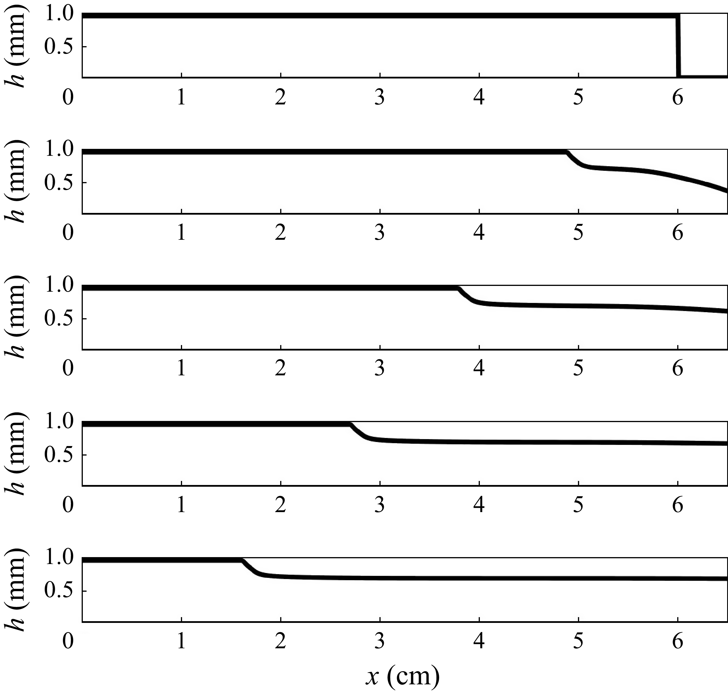
 t=0
 t=0.15
 t=0.3
 t=0.45
 t=0.6


 Open access

