2.1 System configuration

We consider two miscible fluids with molecular weight ratio $W_{2}/W_{1}=3$ , corresponding to an Atwood number

(2.1) $$\begin{eqnarray}\displaystyle At=\frac{W_{2}-W_{1}}{W_{2}+W_{1}} & & \displaystyle\end{eqnarray}$$

of $At=0.5$ . The fluids are contained within a box of length $L\times 2L\times L$ with $L=2\unicode[STIX]{x03C0}$ . Gravity $g$ is aligned in the negative $y$ -direction. Periodic boundary conditions are imposed in the homogeneous $x$ - and $z$ -directions. A no-slip wall is enforced at the upper and lower boundaries, i.e. $y=\pm 2\unicode[STIX]{x03C0}$ . The reference velocity is taken to be $u_{\infty }=\sqrt{gl}$ with the reference length scale $l=L/2\unicode[STIX]{x03C0}$ , resulting in a Froude number $Fr={u_{\infty }}^{2}/(gl)=1$ . The subscript $\infty$ denotes a reference quantity throughout the remainder of this paper.

The domain is discretized on a mesh with $256\times 1025\times 256$ grid points, corresponding to grid spacing $\unicode[STIX]{x0394}x=\unicode[STIX]{x0394}z=0.025l$ in the horizontal directions and $\unicode[STIX]{x0394}y=0.012l$ in the vertical direction. The average kinematic viscosity at the interface $\bar{\unicode[STIX]{x1D708}}$ is chosen such that the Kolmogorov length scale $\unicode[STIX]{x1D702}$ is properly resolved, as determined by the Reynolds number

(2.2) $$\begin{eqnarray}\displaystyle Re=\frac{u_{\infty }l}{\bar{\unicode[STIX]{x1D708}}}=\left(\frac{l}{\unicode[STIX]{x1D702}}\right)^{4/3}, & & \displaystyle\end{eqnarray}$$

which is taken to be $Re=353.3$ with $\unicode[STIX]{x1D702}=\unicode[STIX]{x0394}x/2$ . The average kinematic viscosity is related to the light ( $\unicode[STIX]{x1D707}_{1}$ ) and heavy ( $\unicode[STIX]{x1D707}_{2}$ ) fluid viscosities via $\bar{\unicode[STIX]{x1D708}}=(\unicode[STIX]{x1D707}_{1}+\unicode[STIX]{x1D707}_{2})/(\unicode[STIX]{x1D70C}_{1}+\unicode[STIX]{x1D70C}_{2})$ , where $\unicode[STIX]{x1D70C}_{1}$ and $\unicode[STIX]{x1D70C}_{2}$ are the densities of the fluid below and above the interface, respectively. The dynamic viscosity of the mixture, $\unicode[STIX]{x1D707}$ , is taken to be constant, i.e. $\unicode[STIX]{x1D707}=\unicode[STIX]{x1D707}_{1}=\unicode[STIX]{x1D707}_{2}=\unicode[STIX]{x1D707}_{\infty }$ .

2.2 Governing equations

In this work, we consider the non-dimensional Navier–Stokes equations for a two-component fluid, given by

(2.3) $$\begin{eqnarray}\displaystyle & \displaystyle \frac{\unicode[STIX]{x2202}\unicode[STIX]{x1D70C}}{\unicode[STIX]{x2202}t}+\frac{\unicode[STIX]{x2202}\left(\unicode[STIX]{x1D70C}u_{j}\right)}{\unicode[STIX]{x2202}x_{j}}=0, & \displaystyle\end{eqnarray}$$

(2.4) $$\begin{eqnarray}\displaystyle & \displaystyle \frac{\unicode[STIX]{x2202}\left(\unicode[STIX]{x1D70C}u_{i}\right)}{\unicode[STIX]{x2202}t}+\frac{\unicode[STIX]{x2202}}{\unicode[STIX]{x2202}x_{j}}\left(\unicode[STIX]{x1D70C}u_{i}u_{j}+p\unicode[STIX]{x1D6FF}_{ij}\right)=\frac{\unicode[STIX]{x2202}\unicode[STIX]{x1D70F}_{ij}}{\unicode[STIX]{x2202}x_{j}}-\frac{\unicode[STIX]{x1D70C}}{Fr_{c}}\unicode[STIX]{x1D6FF}_{2i}, & \displaystyle\end{eqnarray}$$

(2.5) $$\begin{eqnarray}\displaystyle & \displaystyle \frac{\unicode[STIX]{x2202}\left(\unicode[STIX]{x1D70C}E\right)}{\unicode[STIX]{x2202}t}+\frac{\unicode[STIX]{x2202}}{\unicode[STIX]{x2202}x_{j}}\left[\left(\unicode[STIX]{x1D70C}E+p\right)u_{j}\right]=-\frac{\unicode[STIX]{x2202}q_{j}}{\unicode[STIX]{x2202}x_{j}}+\frac{\unicode[STIX]{x2202}\left(u_{i}\unicode[STIX]{x1D70F}_{ij}\right)}{\unicode[STIX]{x2202}x_{j}}-\frac{\unicode[STIX]{x1D70C}u_{2}}{Fr_{c}}, & \displaystyle\end{eqnarray}$$

(2.6) $$\begin{eqnarray}\displaystyle & \displaystyle \frac{\unicode[STIX]{x2202}\left(\unicode[STIX]{x1D70C}Y\right)}{\unicode[STIX]{x2202}t}+\frac{\unicode[STIX]{x2202}\left(\unicode[STIX]{x1D70C}u_{j}Y\right)}{\unicode[STIX]{x2202}x_{j}}=\frac{1}{Re_{c}Sc}\frac{\unicode[STIX]{x2202}^{2}Y}{\unicode[STIX]{x2202}x_{j}\unicode[STIX]{x2202}x_{j}}, & \displaystyle\end{eqnarray}$$

for the non-dimensional conserved variables $\boldsymbol{Q}=[\unicode[STIX]{x1D70C}\,\,\unicode[STIX]{x1D70C}\boldsymbol{u}\,\,\unicode[STIX]{x1D70C}E\,\,\unicode[STIX]{x1D70C}Y]^{\text{T}}$ , where $\unicode[STIX]{x1D70C}$ is the mixture density, $\boldsymbol{u}=[u\,\,v\,\,w]^{\text{T}}$ is the velocity vector, $E$ is the total non-chemical energy (including thermal and kinetic energy), $Y$ is the heavy fluid mass fraction with $1-Y$ the mass fraction of the light fluid and $p$ is the pressure given by

(2.7) $$\begin{eqnarray}p=\left(\unicode[STIX]{x1D6FE}-1\right)(\unicode[STIX]{x1D70C}E-{\textstyle \frac{1}{2}}\unicode[STIX]{x1D70C}u_{i}u_{i}),\end{eqnarray}$$

where $\unicode[STIX]{x1D6FE}=1.4$ is the specific heat ratio. In (2.4)–(2.6), $Fr_{c}=Fr/Ma^{2}$ and $Re_{c}=Re/Ma$ denote the Froude and Reynolds numbers, respectively, based on the reference sound speed $c_{\infty }=\sqrt{\unicode[STIX]{x1D6FE}p_{I}/\unicode[STIX]{x1D70C}_{I}}$ with interfacial pressure $p_{I}$ and density $\unicode[STIX]{x1D70C}_{I}=(\unicode[STIX]{x1D70C}_{1}+\unicode[STIX]{x1D70C}_{2})/2$ . The Mach number $Ma=u_{\infty }/c_{\infty }=0.189$ is taken such that compressibility effects on the RT instability are not important (Livescu Reference Livescu2004). The non-dimensional viscous stress tensor $\unicode[STIX]{x1D70F}_{ij}$ is given by

(2.8) $$\begin{eqnarray}\displaystyle \unicode[STIX]{x1D70F}_{ij}=\frac{1}{Re_{c}}\left(\frac{\unicode[STIX]{x2202}u_{i}}{\unicode[STIX]{x2202}x_{j}}+\frac{\unicode[STIX]{x2202}u_{j}}{\unicode[STIX]{x2202}x_{i}}-\frac{2}{3}\frac{\unicode[STIX]{x2202}u_{k}}{\unicode[STIX]{x2202}x_{k}}\unicode[STIX]{x1D6FF}_{ij}\right), & & \displaystyle\end{eqnarray}$$

and the non-dimensional heat flux is expressed as

(2.9) $$\begin{eqnarray}\displaystyle q_{i}=-\frac{1}{Re_{c}Pr}\frac{\unicode[STIX]{x2202}T}{\unicode[STIX]{x2202}x_{i}}-\frac{T}{Re_{c}Sc}\left[\frac{1}{W_{1}}\frac{\unicode[STIX]{x2202}(1-Y)}{\unicode[STIX]{x2202}x_{i}}+\frac{1}{W_{2}}\frac{\unicode[STIX]{x2202}Y}{\unicode[STIX]{x2202}x_{i}}\right], & & \displaystyle\end{eqnarray}$$

where $T$ is the temperature that is determined by the ideal gas law for a mixture

(2.10) $$\begin{eqnarray}\displaystyle T=\frac{\unicode[STIX]{x1D6FE}p\overline{W}}{(\unicode[STIX]{x1D6FE}-1)\unicode[STIX]{x1D70C}}, & & \displaystyle\end{eqnarray}$$

where $\overline{W}$ denotes the mixture molecular weight, given by

(2.11) $$\begin{eqnarray}\displaystyle \overline{W}=\left(\frac{Y}{W_{2}}+\frac{1-Y}{W_{1}}\right)^{-1}. & & \displaystyle\end{eqnarray}$$

In (2.9), $\mathit{Pr}=C_{p,\infty }\unicode[STIX]{x1D707}/k$ is the Prandtl number with $k$ and $C_{p,\infty }$ the thermal conductivity and reference specific heat at constant pressure, respectively, and $Sc=\unicode[STIX]{x1D707}/(\unicode[STIX]{x1D70C}D)$ is the Schmidt number with mass diffusivity $D$ . Values of $k/C_{p,\infty }$ and $\unicode[STIX]{x1D70C}D$ are chosen to be constant such that $\mathit{Pr}=0.7$ and $Sc=1$ .

2.3 Initialization

The mole fraction of the heavy fluid, $X=Y\overline{W}/W_{2}$ , is initialized as

(2.12) $$\begin{eqnarray}\displaystyle X=\frac{1}{2}\left\{1+\operatorname{erf}\left[\frac{y-h_{0}(x,z)}{\unicode[STIX]{x1D6FF}_{D}}\right]\right\}, & & \displaystyle\end{eqnarray}$$

where $\unicode[STIX]{x1D6FF}_{D}=5\unicode[STIX]{x0394}y$ is the initial diffusion thickness of the interface, and $h_{0}(x,z)$ denotes the interfacial perturbations, composed of $M$ modes in the $x$ -direction and $N$ modes in the $z$ -direction, according to

(2.13) $$\begin{eqnarray}\displaystyle h_{0}(x,z)=\mathop{\sum }_{m=1}^{M}\mathop{\sum }_{n=1}^{N}A_{m,n}\cos (k_{x,m}x+\unicode[STIX]{x1D703}_{x,m})\cos (k_{z,n}z+\unicode[STIX]{x1D703}_{z,n}). & & \displaystyle\end{eqnarray}$$

Here, $k_{x,m}=2\unicode[STIX]{x03C0}/\unicode[STIX]{x1D706}_{x,m}$ and $k_{z,n}=2\unicode[STIX]{x03C0}/\unicode[STIX]{x1D706}_{z,n}$ are the perturbation wavenumbers with wavelengths $\unicode[STIX]{x1D706}_{x,m}$ and $\unicode[STIX]{x1D706}_{z,n}$ in $x$ - and $z$ -direction, respectively, with phase shift $\unicode[STIX]{x1D703}_{x,m}$ and $\unicode[STIX]{x1D703}_{z,n}$ , and amplitude $A_{m,n}$ .

The fluid is taken to be initially at rest, i.e. $u_{i}=0$ , and thus the momentum conservation equation (2.4) provides a hydrostatic relation for pressure, given by $\unicode[STIX]{x2202}p/\unicode[STIX]{x2202}y=-\unicode[STIX]{x1D70C}/Fr_{c}$ . Substituting $\unicode[STIX]{x1D70C}$ for $p$ in the hydrostatic equation via (2.10) and integrating from $y=h_{0}(x,z)$ to an arbitrary vertical position $y$ yields

(2.14) $$\begin{eqnarray}\displaystyle p & = & \displaystyle p_{I}\exp \left(-\frac{\unicode[STIX]{x1D6FE}}{(\unicode[STIX]{x1D6FE}-1)T_{0}}\frac{1}{Fr_{c}}\right.\vphantom{\left\{\exp \left[-\frac{(y-h_{0})^{2}}{\unicode[STIX]{x1D6FF}_{D}^{2}}\right]-1\right\}}\nonumber\\ \displaystyle & & \displaystyle \times \,\left.\left[\overline{W}\left(y-h_{0}\right)+\frac{\unicode[STIX]{x1D6FF}_{D}\left(W_{2}-W_{1}\right)}{2\sqrt{\unicode[STIX]{x03C0}}}\left\{\exp \left[-\frac{(y-h_{0})^{2}}{\unicode[STIX]{x1D6FF}_{D}^{2}}\right]-1\right\}\right]\right).\end{eqnarray}$$

Here, $p_{I}$ is the fluid interface pressure and $T_{0}$ denotes the initial temperature that is assumed to be constant throughout the entire domain, resulting in an initially isothermal state. The density is initialized by substituting the resulting pressure into (2.10). It is important to note that employing stationary initial conditions with the hydrostatic pressure distribution $\unicode[STIX]{x2202}p/\unicode[STIX]{x2202}y=-\unicode[STIX]{x1D70C}/Fr_{c}$ will generate spurious acoustic waves near the interface. These waves originate from pressure disturbances as a result of non-zero enthalpy diffusion that appears in the energy equation (Cook Reference Cook2009; Livescu Reference Livescu2013; Reckinger, Livescu & Vasilyev Reference Reckinger, Livescu and Vasilyev2016). Recent work has shown that the spurious waves can be suppressed by modifying the velocity field near the interface (Movahed Reference Movahed2014; Reckinger et al. Reference Reckinger, Livescu and Vasilyev2016). In the current work, we follow a similar approach described by Reckinger et al. (Reference Reckinger, Livescu and Vasilyev2016) to eliminate these spurious oscillations, resulting in the following initial velocity

(2.15) $$\begin{eqnarray}\displaystyle u_{i}=-\frac{1}{Re_{c}Sc}\frac{1}{\unicode[STIX]{x1D70C}\overline{W}}\frac{\unicode[STIX]{x2202}\overline{W}}{\unicode[STIX]{x2202}x_{i}}. & & \displaystyle\end{eqnarray}$$

2.4 Discretization of the governing equations

In the present work, spatial derivatives appearing in the governing equations (2.3)–(2.6) and (2.8)–(2.9) are obtained via a narrow-stencil finite difference operator that satisfies the summation-by-part (SBP) property (Kreiss & Scherer Reference Kreiss and Scherer1974; Strand Reference Strand1994). We employ spatial derivatives with eighth-order accuracy in the interior domain and fourth order near the boundaries, resulting in fifth-order global accuracy. Second and mixed derivatives are obtained by applying the first derivative consecutively. Sixth-order SBP dissipation operators (Mattsson, Svärd & Nordström Reference Mattsson, Svärd and Nordström2004; Vishnampet Ganapathi Subramanian Reference Vishnampet Ganapathi Subramanian2015) are employed to damp spurious numerical waves that arise due to repeated first derivatives. The flow equations are integrated in time using a standard fourth-order Runge–Kutta scheme. A constant simulation timestep of $\unicode[STIX]{x0394}t=2.67^{-4}\unicode[STIX]{x1D70F}$ with $\unicode[STIX]{x1D70F}=\sqrt{Fr_{c}L/l\,At}$ a characteristic time scale is maintained such that the Courant–Friedrichs–Lewy (CFL) condition remains below $\text{CFL}<0.9$ .

The SBP scheme is combined with the simultaneous-approximation-term (SAT) boundary treatment to ensure provable stability (Carpenter, Gottlieb & Abarbanel Reference Carpenter, Gottlieb and Abarbanel1994; Svärd & Nordström Reference Svärd and Nordström2008; Bodony Reference Bodony2010; Vishnampet Ganapathi Subramanian Reference Vishnampet Ganapathi Subramanian2015). The SAT treatment is used to impose no-slip isothermal boundary conditions at $y=\pm 2\unicode[STIX]{x03C0}$ (Svärd & Nordström Reference Svärd and Nordström2008; Vishnampet Ganapathi Subramanian Reference Vishnampet Ganapathi Subramanian2015). In addition, absorbing sponge regions (Freund Reference Freund1997) are applied near the walls by adding a damping term to suppress numerical acoustic waves and to enforce the solution to a target state $\boldsymbol{Q}_{t}$ (taken to be the unperturbed initial conditions). The damping term $\unicode[STIX]{x1D70E}_{s}(y)(\boldsymbol{Q}-\boldsymbol{Q}_{t})$ is added to the right-hand side of the governing equations (2.3)–(2.6), where the sponge strength $\unicode[STIX]{x1D70E}_{s}(y)$ varies quadratically in the $y$ -direction from unity at the walls to zero at ${\approx}0.7l$ away from the wall.

3.1 A background on Rayleigh–Taylor growth

RT instabilities are known to undergo a range of stages during their growth. In the limit that either the Schmidt number, the perturbation amplitude or gravity is sufficiently small, the initial growth will be dominated by diffusion (Duff et al. Reference Duff, Harlow and Hirt1962; Cook & Dimotakis Reference Cook and Dimotakis2001; Wei & Livescu Reference Wei and Livescu2012). Following diffusional growth, the perturbation amplitude grows exponentially with time according to linear stability theory (Chandrasekhar Reference Chandrasekhar1961; Duff et al. Reference Duff, Harlow and Hirt1962; Livescu Reference Livescu2004). The exponential growth holds when the perturbation amplitude $h$ is significantly smaller than the perturbation wavelength $\unicode[STIX]{x1D706}$ , i.e. $h\ll \unicode[STIX]{x1D706}$ . When $h$ is not sufficiently small, nonlinearities become important, and bubbles and spikes form as the two fluids penetrate each other, resulting in a growing mixing zone. During the nonlinear regime, the bubble tip velocity of a single-mode RT instability is known to reach a constant value proportional to $\sqrt{g\unicode[STIX]{x1D706}}$  (Layzer Reference Layzer1955; Baker & Freeman Reference Baker and Freeman1981; Hecht, Alon & Shvarts Reference Hecht, Alon and Shvarts1994; Goncharov Reference Goncharov2002). After sufficiently long time, the mixing zone grows quadratically (Anuchina et al. Reference Anuchina, Kucherenko, Neuvazhaev, Ogibina, Shibarshov and Yakovlev1978; Youngs Reference Youngs1984), and the acceleration of bubbles and spikes becomes constant, given by (Read Reference Read1984; Youngs Reference Youngs1984)

(3.1) $$\begin{eqnarray}\displaystyle h_{b/s}(t)=\unicode[STIX]{x1D6FC}_{b/s}At\,gt^{2}, & & \displaystyle\end{eqnarray}$$

where indices ‘ $b$ ’ and ‘ $s$ ’ denote bubbles and spikes, respectively, and $\unicode[STIX]{x1D6FC}$ is the growth parameter. There are two primary mechanisms responsible for bubbles approaching self-similarity. The first mechanism, referred to as bubble competition, suggests that each ambient mode grows independently and exponentially until reaching its saturation limit, resulting in a set of saturated bubbles (Alon et al. Reference Alon, Hecht, Mukamel and Shvarts1994; Hecht et al. Reference Hecht, Alon and Shvarts1994; Dimonte Reference Dimonte2004; Ramaprabhu et al. Reference Ramaprabhu, Dimonte and Andrews2005; Banerjee & Andrews Reference Banerjee and Andrews2009). Such a mechanism results in a weak correlation between $\unicode[STIX]{x1D6FC}_{b}$ and the amplitudes of the interfacial perturbations (Dimonte Reference Dimonte2004; Ramaprabhu et al. Reference Ramaprabhu, Dimonte and Andrews2005; Banerjee & Andrews Reference Banerjee and Andrews2009). The second mechanism, referred to as bubble merger, suggests that different bubbles merge and couple nonlinearly to create larger and faster bubbles (Sharp Reference Sharp1984; Alon et al. Reference Alon, Hecht, Mukamel and Shvarts1994; Dimonte Reference Dimonte2004; Dimonte et al. Reference Dimonte, Youngs, Dimits, Weber, Marinak, Wunsch, Garasi, Robinson, Andrews and Ramaprabhu2004; Ramaprabhu et al. Reference Ramaprabhu, Dimonte and Andrews2005; Banerjee & Andrews Reference Banerjee and Andrews2009). In contrast to bubble competition, the resulting $\unicode[STIX]{x1D6FC}_{b}$ of pure mode coupling does not depend on initial perturbations (Alon et al. Reference Alon, Hecht, Mukamel and Shvarts1994; Dimonte et al. Reference Dimonte, Youngs, Dimits, Weber, Marinak, Wunsch, Garasi, Robinson, Andrews and Ramaprabhu2004; Ramaprabhu et al. Reference Ramaprabhu, Dimonte and Andrews2005; Banerjee & Andrews Reference Banerjee and Andrews2009). Thus, no universal value for $\unicode[STIX]{x1D6FC}$ exists, and a wide range of growth parameters have been reported from experiments and numerical simulations, ranging from $0.015\lessapprox \unicode[STIX]{x1D6FC}\lessapprox 0.085$ (Dimonte et al. Reference Dimonte, Youngs, Dimits, Weber, Marinak, Wunsch, Garasi, Robinson, Andrews and Ramaprabhu2004; Ramaprabhu et al. Reference Ramaprabhu, Dimonte and Andrews2005). In order to more effectively control RT instabilities, it is important to identify to what extent $\unicode[STIX]{x1D6FC}$ is influenced by the structure of the initial interfacial perturbations.

3.2 Quantifying mixing

In this work, the objective function, ${\mathcal{J}}$ , is defined within the simulation domain $\mathbb{D}$ and time horizon $[0,t_{f}]$ as

(3.2) $$\begin{eqnarray}\displaystyle {\mathcal{J}}(\boldsymbol{Q},\boldsymbol{A})=\int _{0}^{t_{f}}\int _{\mathbb{D}}{\mathcal{I}}(\boldsymbol{Q},\boldsymbol{A}){\mathcal{W}}(y)\,\text{d}\boldsymbol{x}\,\text{d}t, & & \displaystyle\end{eqnarray}$$

where the integrand ${\mathcal{I}}$ denotes the local temporal mixing provided by a high-fidelity simulation that solves the governing equations (2.3)–(2.6), and $\boldsymbol{A}=[A_{1,1},\ldots ,~A_{M,N}]^{\text{T}}$ . The weighting function ${\mathcal{W}}(y)$ enforces compact support near the interface and smoothly decays to zero towards the vertical boundaries, given by

(3.3) $$\begin{eqnarray}\displaystyle {\mathcal{W}}(y)={\textstyle \frac{1}{2}}\left\{\tanh \left[\unicode[STIX]{x1D70E}_{{\mathcal{W}}}\left(y+1-f_{{\mathcal{W}}}/2\right)\right]-\tanh \left[\unicode[STIX]{x1D70E}_{{\mathcal{W}}}\left(y-1+f_{{\mathcal{W}}}/2\right)\right]\right\}, & & \displaystyle\end{eqnarray}$$

where $\unicode[STIX]{x1D70E}_{{\mathcal{W}}}=25.0/l$ determines the slope, and $f_{{\mathcal{W}}}=0.25l$ controls the fraction of the span for which ${\mathcal{W}}$ is maximum. The choice of these parameters have negligible effect on the results reported here.

The choice of ${\mathcal{I}}$ in (3.2) is critical for measuring mixing and growth of the RT instability. Several definitions for ${\mathcal{I}}$ can be found in the literature. One measure is the bubble–spike distance $h_{t}$  (e.g. see Cook & Dimotakis Reference Cook and Dimotakis2001), given by

(3.4) $$\begin{eqnarray}\displaystyle h_{t}=h_{b}-h_{s}. & & \displaystyle\end{eqnarray}$$

For multi-mode RT instabilities, thresholds on spanwise-averaged mole, volume or mass fraction are typically used to measure bubble and spike heights (e.g. see Cook & Dimotakis Reference Cook and Dimotakis2001; Dimonte et al. Reference Dimonte, Youngs, Dimits, Weber, Marinak, Wunsch, Garasi, Robinson, Andrews and Ramaprabhu2004; Movahed Reference Movahed2014). In the present work, we consider $\langle X\rangle =0.99$ and $\langle X\rangle =0.01$ thresholds for determining bubble $h_{b}$ and spike $h_{s}$ heights, respectively, where $\langle \cdot \rangle$ denotes a spanwise average, given by

(3.5) $$\begin{eqnarray}\displaystyle \langle \unicode[STIX]{x1D719}\rangle (y)=\frac{1}{L^{2}}\int _{-L/2}^{L/2}\int _{-L/2}^{L/2}\unicode[STIX]{x1D719}(x,y,z)\,\text{d}z\,\text{d}x, & & \displaystyle\end{eqnarray}$$

where $\unicode[STIX]{x1D719}$ can be the mole, volume or mass fraction. Another common measure is the mixing width, given by (e.g. see Dimonte et al. Reference Dimonte, Youngs, Dimits, Weber, Marinak, Wunsch, Garasi, Robinson, Andrews and Ramaprabhu2004; Cabot Reference Cabot2006)

(3.6) $$\begin{eqnarray}\displaystyle w=\int _{-L}^{L}\left\langle \unicode[STIX]{x1D719}\right\rangle \left(1-\left\langle \unicode[STIX]{x1D719}\right\rangle \right)\text{d}y. & & \displaystyle\end{eqnarray}$$

In addition, mixed fluid can be defined as the product of a hypothetical fast-kinetic reversible chemical reaction between two pure fluids, such that a corresponding mixing length is given by (e.g. see Cook & Dimotakis Reference Cook and Dimotakis2001; Movahed Reference Movahed2014)

(3.7) $$\begin{eqnarray}\displaystyle h_{m}=\int _{-L}^{L}\unicode[STIX]{x1D719}_{m}\left(\left\langle \unicode[STIX]{x1D719}\right\rangle \right)\text{d}y, & & \displaystyle\end{eqnarray}$$

where $h_{m}$ is the mixing height, and $\unicode[STIX]{x1D719}_{m}(\unicode[STIX]{x1D719})$ is a corresponding mixed fluid fraction, where $\unicode[STIX]{x1D719}_{m}=2\unicode[STIX]{x1D719}$ for $\unicode[STIX]{x1D719}\leqslant 0.5$ ; $\unicode[STIX]{x1D719}_{m}=2\left(1-\unicode[STIX]{x1D719}\right)$ otherwise. In the current work, $\left\langle \unicode[STIX]{x1D719}\right\rangle =\left\langle X\right\rangle$ is considered in (3.6) and (3.7).

In the present work, the adjoint of the perturbed and linearized governing equations is solved to determine the sensitivity of mixing and growth, which requires the objective function to be differentiable with respect to flow variables $\boldsymbol{Q}$ and perturbation parameters $\boldsymbol{A}$ . However, computing derivatives of the aforementioned quantities can be problematic, and thus necessitates a new measure of mixing. An initial candidate for ${\mathcal{I}}$ in (3.2) is to utilize the form of (3.6) with ${\mathcal{I}}=X\left(1-X\right)$ , leading to ${\mathcal{J}}$ that quantifies mixing, defined as

(3.8) $$\begin{eqnarray}\displaystyle \text{MIX}=\int _{0}^{t_{f}}\int _{\mathbb{D}}X\left(1-X\right){\mathcal{W}}(y)\,\text{d}\boldsymbol{x}\,\text{d}t, & & \displaystyle\end{eqnarray}$$

in which its maximum value occurs at $X=0.5$ (representing the fully mixed fluid), and $\text{MIX}=0$ within a pure fluid. It is important to note that due to the initial smooth distribution of $X$ as given by (2.12), $\text{MIX}(t=0)\neq 0$ even for an unperturbed interface.

Alternatively, the definition of mixing can be defined based on the perturbation kinetic energy (Aamo, Krstić & Bewley Reference Aamo, Krstić and Bewley2003; Foures et al. Reference Foures, Caulfield and Schmid2014; Lopez-Zazueta et al. Reference Lopez-Zazueta, Fontane and Joly2016; Vermach & Caulfield Reference Vermach and Caulfield2018). Because the interfacial fluid movement is closely related to the local velocity of the interface, it is reasonable to consider an $L^{2}$ -norm of vertical velocity $v$ , resulting in ${\mathcal{J}}$ that quantifies the kinetic energy, given by

(3.9) $$\begin{eqnarray}\displaystyle \text{KE}=\int _{0}^{t_{f}}\int _{\mathbb{D}}v^{2}{\mathcal{W}}(y)\,\text{d}\boldsymbol{x}\,\text{d}t. & & \displaystyle\end{eqnarray}$$

Foures et al. (Reference Foures, Caulfield and Schmid2014) and Vermach & Caulfield (Reference Vermach and Caulfield2018) showed that maximizing the perturbation kinetic energy does not effectively enhance mixing of a passive scalar in plane channel flows. Even so, the utility of this definition for controlling RT growth will be analysed in later sections.

In addition to the definitions above, we consider a third quantity that represents the deviation of mole fraction from its unperturbed initial value $X_{\infty }$ , according to

(3.10) $$\begin{eqnarray}\displaystyle \text{VAR}=\int _{0}^{t_{f}}\int _{\mathbb{D}}\left(X-X_{\infty }\right)^{2}{\mathcal{W}}(y)\,\text{d}\boldsymbol{x}\,\text{d}t, & & \displaystyle\end{eqnarray}$$

where $X_{\infty }$ is determined by (2.12) with $h_{0}(x,z)=0$ . $\text{VAR}$ can be considered as the ‘variance’ of $X$ with respect to the unperturbed field $X_{\infty }$ .

In the present work, we seek the sensitivity of these mixing quantities (3.8)–(3.10) with respect to the initial perturbation amplitude of each mode, $A_{m,n}$ . Considering the variations of ${\mathcal{J}}$ with respect to $\boldsymbol{A}$ , the sensitivity is given by the chain rule as

(3.11) $$\begin{eqnarray}\displaystyle \frac{\unicode[STIX]{x1D6FF}{\mathcal{J}}}{\unicode[STIX]{x1D6FF}\boldsymbol{A}}=\frac{\unicode[STIX]{x2202}{\mathcal{J}}}{\unicode[STIX]{x2202}Q}\frac{\unicode[STIX]{x1D6FF}Q}{\unicode[STIX]{x1D6FF}\boldsymbol{A}}+\frac{\unicode[STIX]{x2202}{\mathcal{J}}}{\unicode[STIX]{x2202}\boldsymbol{A}}, & & \displaystyle\end{eqnarray}$$

where $\unicode[STIX]{x1D6FF}$ denotes small variations. A brute-force approach for evaluating $\unicode[STIX]{x1D6FF}Q/\unicode[STIX]{x1D6FF}\boldsymbol{A}$ would require perturbing each amplitude individually and performing a new simulation for each to measure the change in flow solution $\unicode[STIX]{x1D6FF}Q$ . In this work, that would require $M\times N$ solutions of the time-dependent multi-component Navier–Stokes equations, resulting in a prohibitively large number of simulations. An alternative, more computationally efficient approach is to solve the corresponding adjoint equations by linearizing the perturbed flow equations, which is addressed in the following section.

3.3 Quantifying sensitivity of mixing

The flow variables $\boldsymbol{Q}$ and initial perturbation amplitudes $\boldsymbol{A}$ are governed by the Navier–Stokes equations and its initial conditions, given by

(3.12) $$\begin{eqnarray}\displaystyle \boldsymbol{{\mathcal{M}}}(\boldsymbol{Q},\boldsymbol{A})=\boldsymbol{{\mathcal{N}}}(\boldsymbol{Q})+\left[\boldsymbol{Q}(\boldsymbol{A})-\boldsymbol{Q}_{0}\right]\unicode[STIX]{x1D6FF}_{t=0}\equiv 0, & & \displaystyle\end{eqnarray}$$

where $\boldsymbol{{\mathcal{N}}}$ denotes the flow equations (2.3)–(2.6), $\boldsymbol{Q}_{0}(\boldsymbol{A})$ are the flow variables at $t=0$ and $\unicode[STIX]{x1D6FF}_{t=0}$ denotes the Dirac Delta function, which is unity for $t=0$ and zero otherwise. The last term in (3.12) enforces the initial conditions and is presented as such to obtain the sensitivity of ${\mathcal{J}}$ to $\boldsymbol{A}$ . A similar formulation can be found in Foures et al. (Reference Foures, Caulfield and Schmid2014). The Lagrangian ${\mathcal{L}}$ of ${\mathcal{J}}$ constrained by $\boldsymbol{{\mathcal{M}}}$ is given by

(3.13) $$\begin{eqnarray}\displaystyle {\mathcal{L}}(\boldsymbol{Q},\boldsymbol{A})={\mathcal{J}}(\boldsymbol{Q},\boldsymbol{A})-\int _{0}^{t_{f}}\int _{\mathbb{D}}\boldsymbol{Q}^{\dagger \text{T}}\boldsymbol{{\mathcal{M}}}(\boldsymbol{Q},\boldsymbol{A})\,\text{d}\boldsymbol{x}\,\text{d}t, & & \displaystyle\end{eqnarray}$$

where $\boldsymbol{Q}^{\dagger }=[\unicode[STIX]{x1D70C}^{\dagger }\,\,\boldsymbol{u}^{\dagger }\,\,E^{\dagger }\,\,Y^{\dagger }]^{\text{T}}$ with $\boldsymbol{u}^{\dagger }=[u^{\dagger }\,\,v^{\dagger }\,\,w^{\dagger }]^{\text{T}}$ is the Lagrange multiplier, referred to here as the adjoint variable. Variations of ${\mathcal{L}}$ are expressed as

(3.14) $$\begin{eqnarray}\displaystyle \unicode[STIX]{x1D6FF}{\mathcal{L}}(\boldsymbol{Q},\boldsymbol{A}) & = & \displaystyle \unicode[STIX]{x1D6FF}{\mathcal{J}}(\boldsymbol{Q},\boldsymbol{A})-\int _{0}^{t_{f}}\int _{\mathbb{D}}\unicode[STIX]{x1D6FF}\boldsymbol{Q}^{\dagger \text{T}}\boldsymbol{{\mathcal{M}}}(\boldsymbol{Q},\boldsymbol{A})\,\text{d}\boldsymbol{x}\,\text{d}t\nonumber\\ \displaystyle & & \displaystyle -\,\int _{0}^{t_{f}}\int _{\mathbb{D}}\boldsymbol{Q}^{\dagger \text{T}}\unicode[STIX]{x1D6FF}\boldsymbol{{\mathcal{M}}}(\boldsymbol{Q},\boldsymbol{A})\,\text{d}\boldsymbol{x}\,\text{d}t.\end{eqnarray}$$

The last two terms on the right-hand side of (3.14) are always zero according to (3.12), leading to $\unicode[STIX]{x1D6FF}{\mathcal{L}}=\unicode[STIX]{x1D6FF}{\mathcal{J}}$ . Taking variations of $\unicode[STIX]{x1D6FF}{\mathcal{J}}$ and $\unicode[STIX]{x1D6FF}{\mathcal{M}}$ and substituting them into (3.14) yields

(3.15) $$\begin{eqnarray}\displaystyle \unicode[STIX]{x1D6FF}{\mathcal{J}} & = & \displaystyle \int _{0}^{t_{f}}\int _{\mathbb{D}}\left[\left(\frac{\unicode[STIX]{x2202}{\mathcal{I}}}{\unicode[STIX]{x2202}\boldsymbol{Q}}\right)^{\text{T}}\unicode[STIX]{x1D6FF}\boldsymbol{Q}{\mathcal{W}}-\boldsymbol{Q}^{\dagger \text{T}}\unicode[STIX]{x1D6FF}\boldsymbol{{\mathcal{N}}}-\boldsymbol{Q}^{\dagger \text{T}}\unicode[STIX]{x1D6FF}\boldsymbol{Q}\unicode[STIX]{x1D6FF}_{t=0}\right]\text{d}\boldsymbol{x}\,\text{d}t\nonumber\\ \displaystyle & & \displaystyle +\,\int _{0}^{t_{f}}\int _{\mathbb{D}}\left[\left(\frac{\unicode[STIX]{x2202}{\mathcal{I}}}{\unicode[STIX]{x2202}\boldsymbol{A}}\right)^{\text{T}}{\mathcal{W}}+\boldsymbol{Q}^{\dagger \text{T}}\frac{\unicode[STIX]{x2202}\boldsymbol{Q}_{0}}{\unicode[STIX]{x2202}\boldsymbol{A}}\unicode[STIX]{x1D6FF}_{t=0}\right]\unicode[STIX]{x1D6FF}\boldsymbol{A}\,\text{d}\boldsymbol{x}\,\text{d}t,\end{eqnarray}$$

where $\unicode[STIX]{x1D6FF}\boldsymbol{{\mathcal{N}}}$ are variations of $\boldsymbol{{\mathcal{N}}}$ with respect to $\boldsymbol{Q}$ . The adjoint variables $\boldsymbol{Q}^{\dagger }$ are chosen such that the first line of (3.15) vanishes, leading to the adjoint partial differential equations provided in appendix A. Putting this together, the sensitivity is computed as

(3.16) $$\begin{eqnarray}\displaystyle \frac{\unicode[STIX]{x1D6FF}{\mathcal{J}}}{\unicode[STIX]{x1D6FF}\boldsymbol{A}}=\int _{\mathbb{D}}\boldsymbol{Q}_{0}^{\dagger \text{T}}\frac{\unicode[STIX]{x2202}\boldsymbol{Q}_{0}}{\unicode[STIX]{x2202}\boldsymbol{A}}\,\text{d}\boldsymbol{x}\quad \text{at}~t=0. & & \displaystyle\end{eqnarray}$$

To avoid measuring sensitivity near the domain boundaries, we multiply a weighting function, ${\mathcal{W}}_{\unicode[STIX]{x1D6E4}}$ , with initial perturbation $h_{0}(x,z)$ that enforces compact support near the interface, and approaches zero towards the walls in a similar manner as (3.3). Therefore, the initial mole fraction equation (2.12) is modified according to

(3.17) $$\begin{eqnarray}\displaystyle X=\frac{1}{2}\left\{1+\operatorname{erf}\left[\frac{y-h_{0}(x,z){\mathcal{W}}_{\unicode[STIX]{x1D6E4}}(y)}{\unicode[STIX]{x1D6FF}_{D}}\right]\right\}. & & \displaystyle\end{eqnarray}$$

This modification does not significantly change the initial conditions provided that the weighting function is near unity in the vicinity of the interface and the imposed perturbation $h_{0}$ is small.

The sensitivity provided by the adjoint solution after discretizing (3.16) can induce truncation errors accumulated in $\boldsymbol{Q}^{\dagger }$ that may become significant in unsteady or chaotic flows (Nadarajah & Jameson Reference Nadarajah and Jameson2000; Carnarius et al. Reference Carnarius, Thiele, Oezkaya and Gauger2010). Simulations of turbulent mixing like the ones considered here are particularly sensitive to this since the numerical resolution is often close to the limits of the discretization. To this end, the present work employs a discrete adjoint method that provides sensitivity with accuracy independent of the underlying numerical scheme and is only limited by machine-precision round-off error. This is achieved by considering the discrete counterpart of the inner product (3.2) and the fully discretized Navier–Stokes equations (in space and time) prior to employing the Lagrangian (3.13). Details of the space–time discrete adjoint formulation consistent with the SBP-SAT discretization outlined in § 2.4, and verification of its sensitivity gradient, can be found in Vishnampet et al. (Reference Vishnampet, Bodony and Freund2015), Capecelatro et al. (Reference Capecelatro, Bodony and Freund2018).

Figure 1.

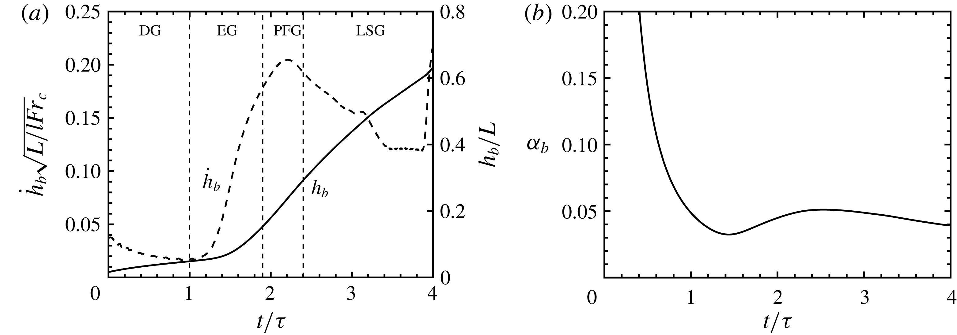
(a) Evolution of bubble height (–) and bubble tip velocity (– –) of the three-dimensional RT instability through the diffusion growth (DG), exponential growth (EG), potential flow growth (PFG) and late-stage growth (LSG). (b) Corresponding bubble growth parameter $\unicode[STIX]{x1D6FC}_{b}$ .

4.1 Rayleigh–Taylor growth

In this section a three-dimensional multi-mode RT instability is considered. The interfacial amplitudes $A_{m,n}$ are initially distributed uniformly, i.e. $A_{m,n}=A_{0}$ for $m=1,\ldots ,M$ and $n=1,\ldots ,N$ , and the phases are distributed randomly, $0\leqslant \unicode[STIX]{x1D703}_{m,x},\unicode[STIX]{x1D703}_{n,z}\leqslant 2\unicode[STIX]{x03C0}$ . Thirty-two modes are considered in each horizontal direction (i.e. $M=N=32$ ), and the smallest wavelength in each direction is $\unicode[STIX]{x1D706}_{min}=8\unicode[STIX]{x0394}x$ . Linear stability theory predicts that the exponential growth rate of the incompressible ( $p_{I}\rightarrow \infty$ ) RT instability is negative for $k>21$  (Duff et al. Reference Duff, Harlow and Hirt1962). Thus, the present configuration should account for all active modes. The root-mean-square (r.m.s.) of initial perturbation $h_{0,rms}=3.15\times 10^{-4}L$ is chosen based on Banerjee & Andrews (Reference Banerjee and Andrews2009), which leads to $A_{0}=1.97\times 10^{-5}L$ .

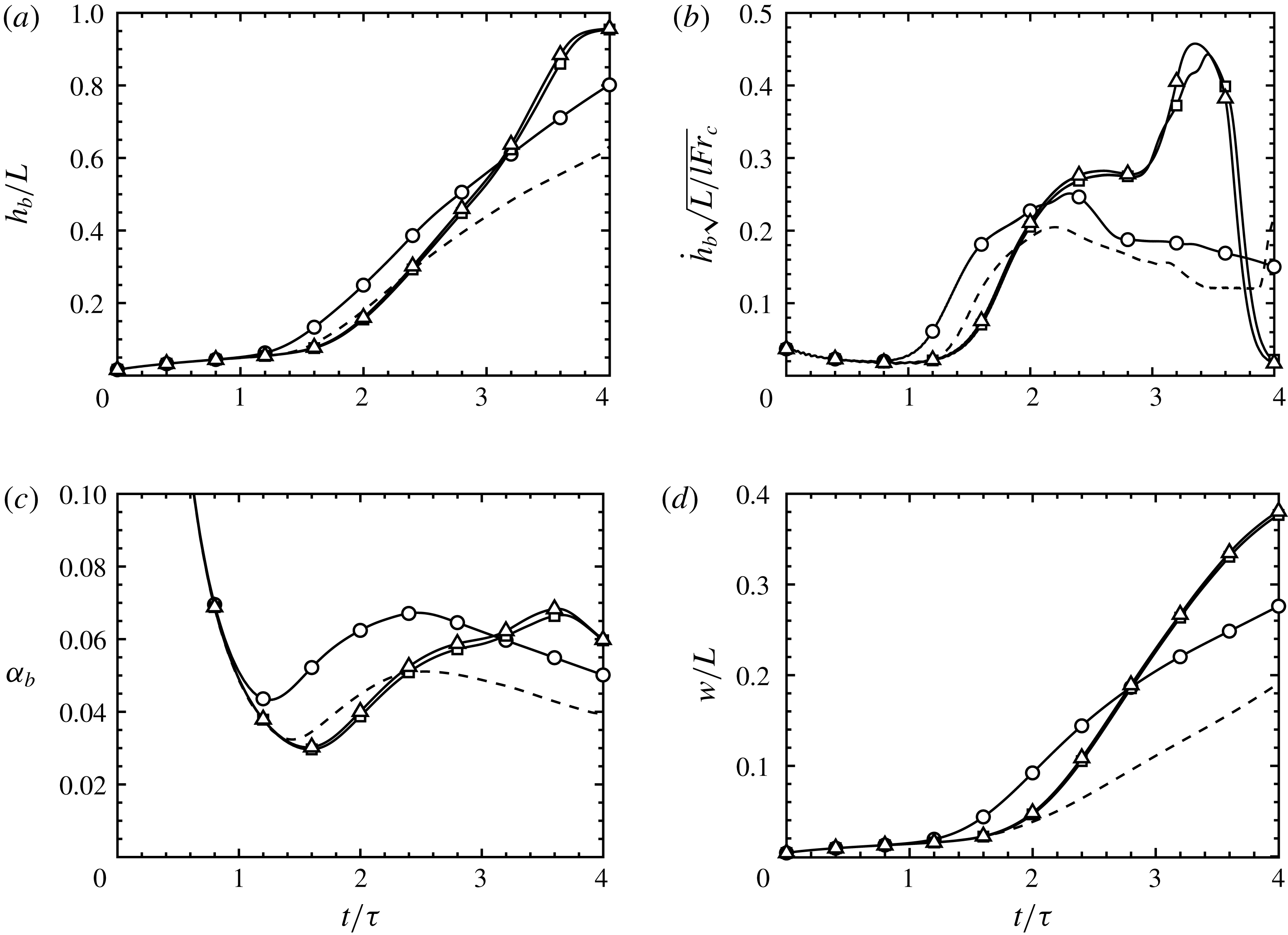
The evolution of bubble height $h_{b}$ and tip velocity ${\dot{h}}_{b}$ in figure 1(a) depict the various stages of RT growth up to $t=4\unicode[STIX]{x1D70F}$ . The instability begins in the diffusion growth (DG) regime until $t\approx \unicode[STIX]{x1D70F}$ . Afterwards, gravitational effects become important, leading to the exponential growth (EG) regime until $t\approx 1.9\unicode[STIX]{x1D70F}$ . Then, nonlinearities become important, giving rise to a potential flow growth (PFG) stage where the bubble tip velocity is approximately constant until $t\approx 2.4\unicode[STIX]{x1D70F}$ . Afterwards, additional nonlinearities cause the bubble tip velocity to decrease. It then reaccelerates at $t\approx 3.9\unicode[STIX]{x1D70F}$ . The corresponding bubble growth parameter becomes approximately constant for $t>2.5\unicode[STIX]{x1D70F}$ , where a self-similar late-stage growth (LSG) regime exists (see figure 1 b). The bubble growth parameter is seen to approach $\unicode[STIX]{x1D6FC}_{b}\approx 0.04$ , consistent with values reported in the literature (e.g. Dimonte et al. Reference Dimonte, Youngs, Dimits, Weber, Marinak, Wunsch, Garasi, Robinson, Andrews and Ramaprabhu2004; Ramaprabhu et al. 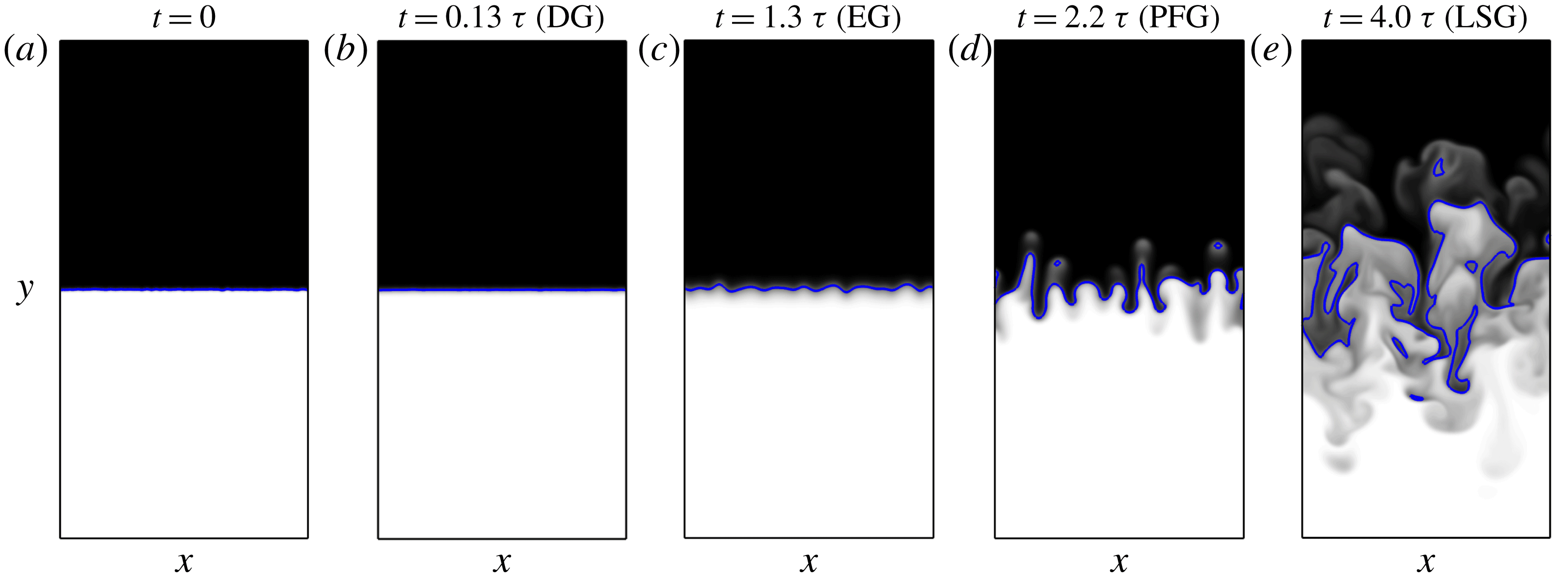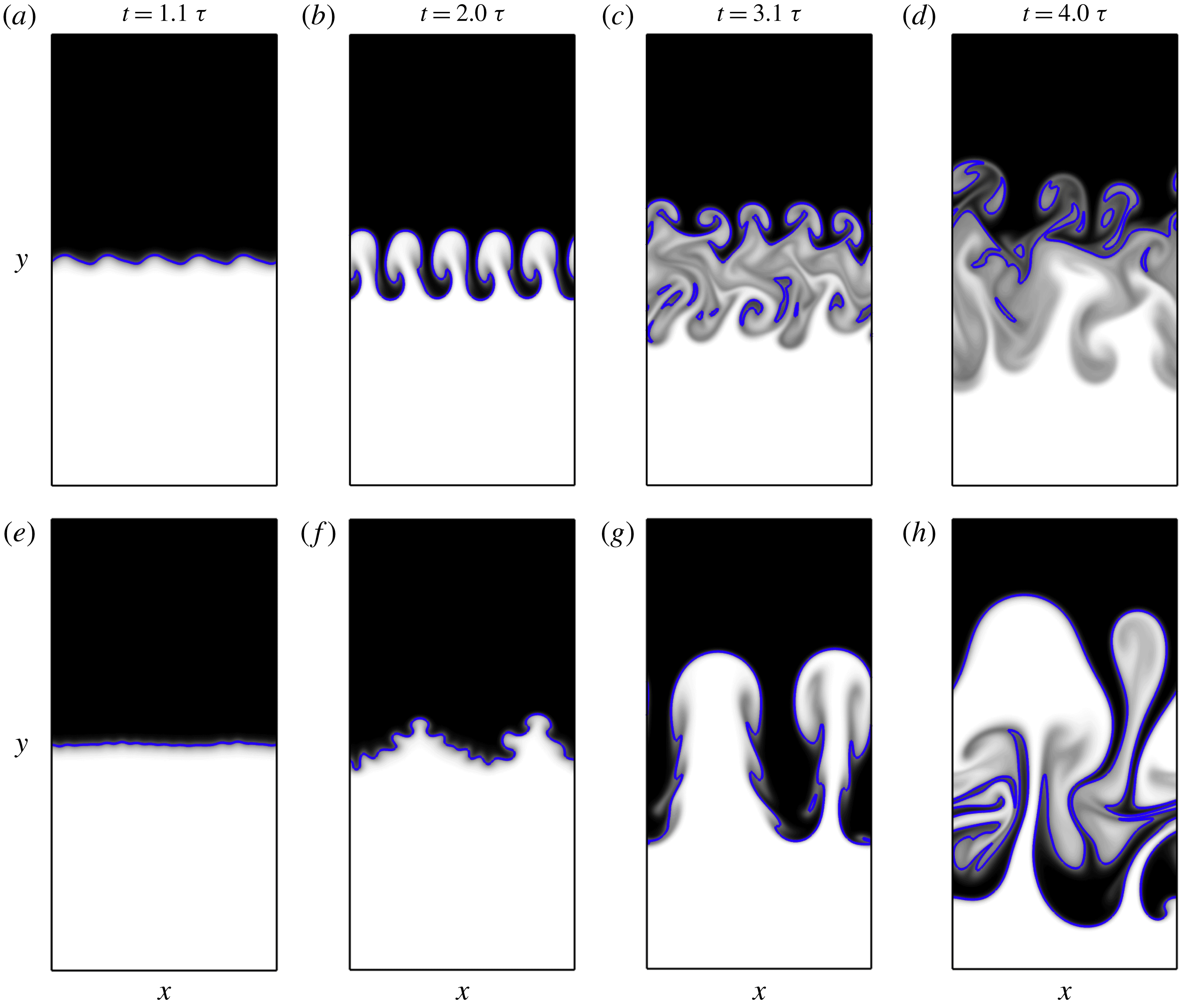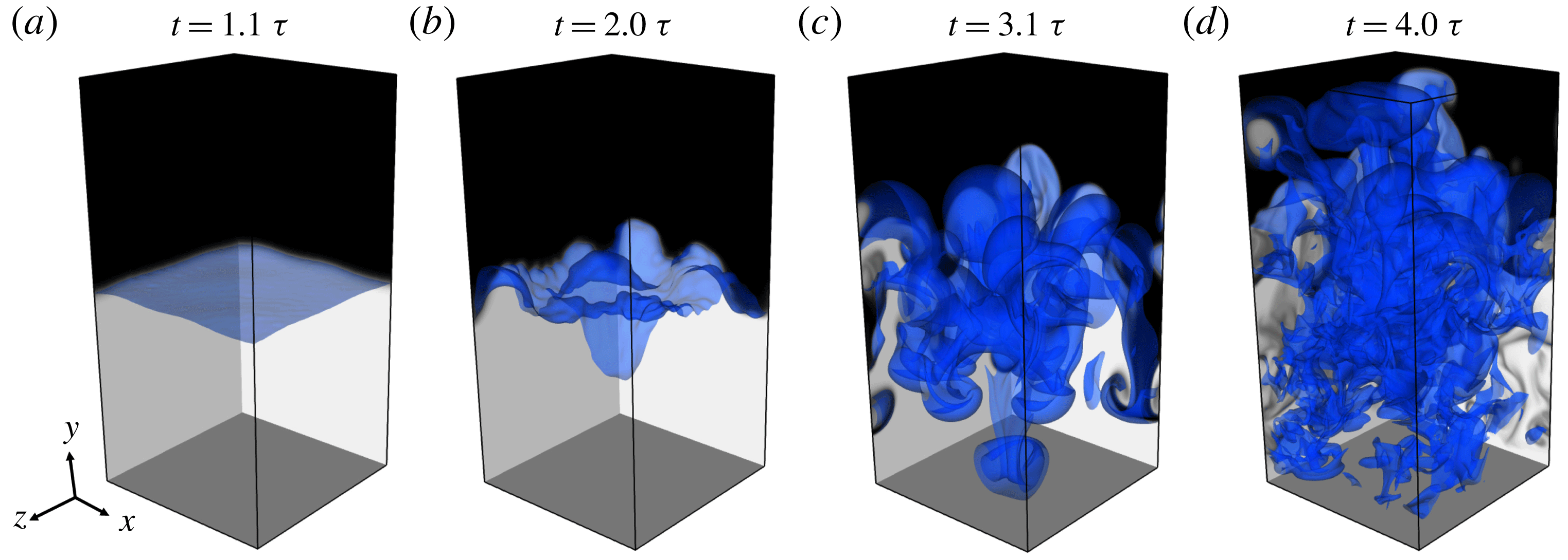Reference Ramaprabhu, Dimonte and Andrews2005). Two-dimensional snapshots of the mole fraction within different regimes do not show significant mixing until reaching the PFG stage (see figure 2).

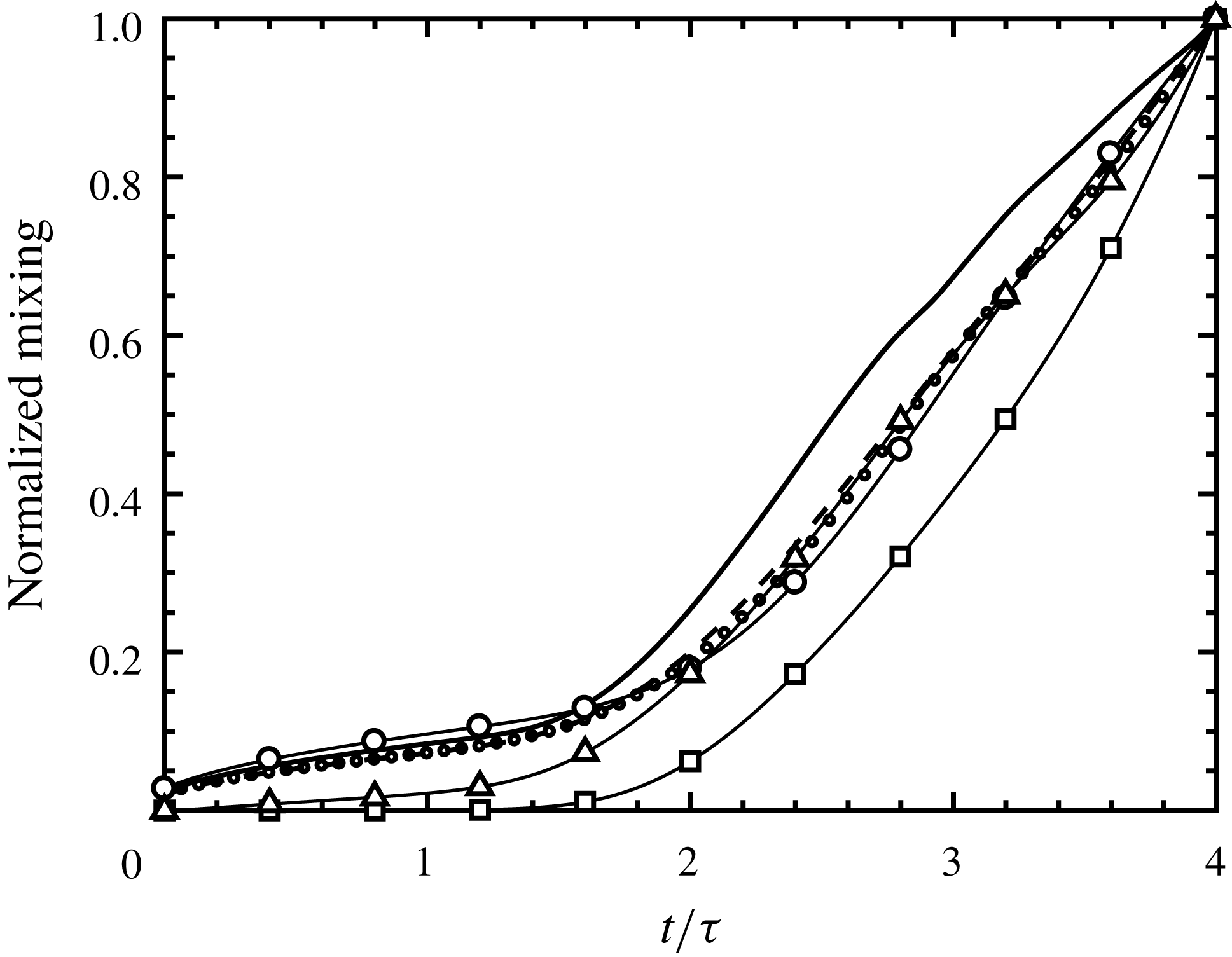
The conventional measures for RT mixing, defined according to (3.4), (3.6) and (3.7), are compared with the objective functions defined in § 3.2 as given by (3.8)–(3.10) (see figure 3). Each quantity shows relatively small growth during the DG and EG stages, and a rapid increase in mixing after $t\approx 2\unicode[STIX]{x1D70F}$ , consistent with figures 1 and 2. It is interesting to note that the trend of each objective function is approximately similar. However, the growth of the kinetic energy norm $\text{KE}$ (defined using ${\mathcal{I}}=v^{2}$ ) is seen to be delayed until $t\approx 2\unicode[STIX]{x1D70F}$ due to diffusion effects. It then increases exponentially according to linear stability theory during the EG regime ( $t\gtrapprox 1.6\unicode[STIX]{x1D70F}$ ). Both $\text{MIX}$ (defined using ${\mathcal{I}}=X(1-X)$ ) and the mixing width $w$ are observed to evolve in a similar manner, which is not unexpected due to their similarities in definition. The initial growth of bubble–spike distance $h_{t}$ is similar to that of the mixing height, mixing width and $\text{MIX}$ . This suggests the objective functions presented in § 3.2 act as good surrogates for quantifying RT growth and mixing. Sensitivity of these quantities to the initial interfacial perturbations will be presented in the following section.

Figure 2.

Evolution of mole fraction $X$ in the $z=-\unicode[STIX]{x03C0}$ plane. The grey scale shows mole fraction from $X=$ 0 (white) to $X=1$ (black). The blue line depicts the fluid interface ( $X=0.5$ ).

Figure 3.

Conventional measures for RT mixing: $h_{t}$ (–), $w$ (– –) and $h_{m}~(\cdots \,)$ . Instantaneous values of the objective functions $\text{MIX}$ (– ○ –), $\text{KE}$ (– ▫ –) and $\text{VAR}$ (– ▵ –). All data are normalized by their final values (at $t=4\unicode[STIX]{x1D70F}$ ).

Figure 4.

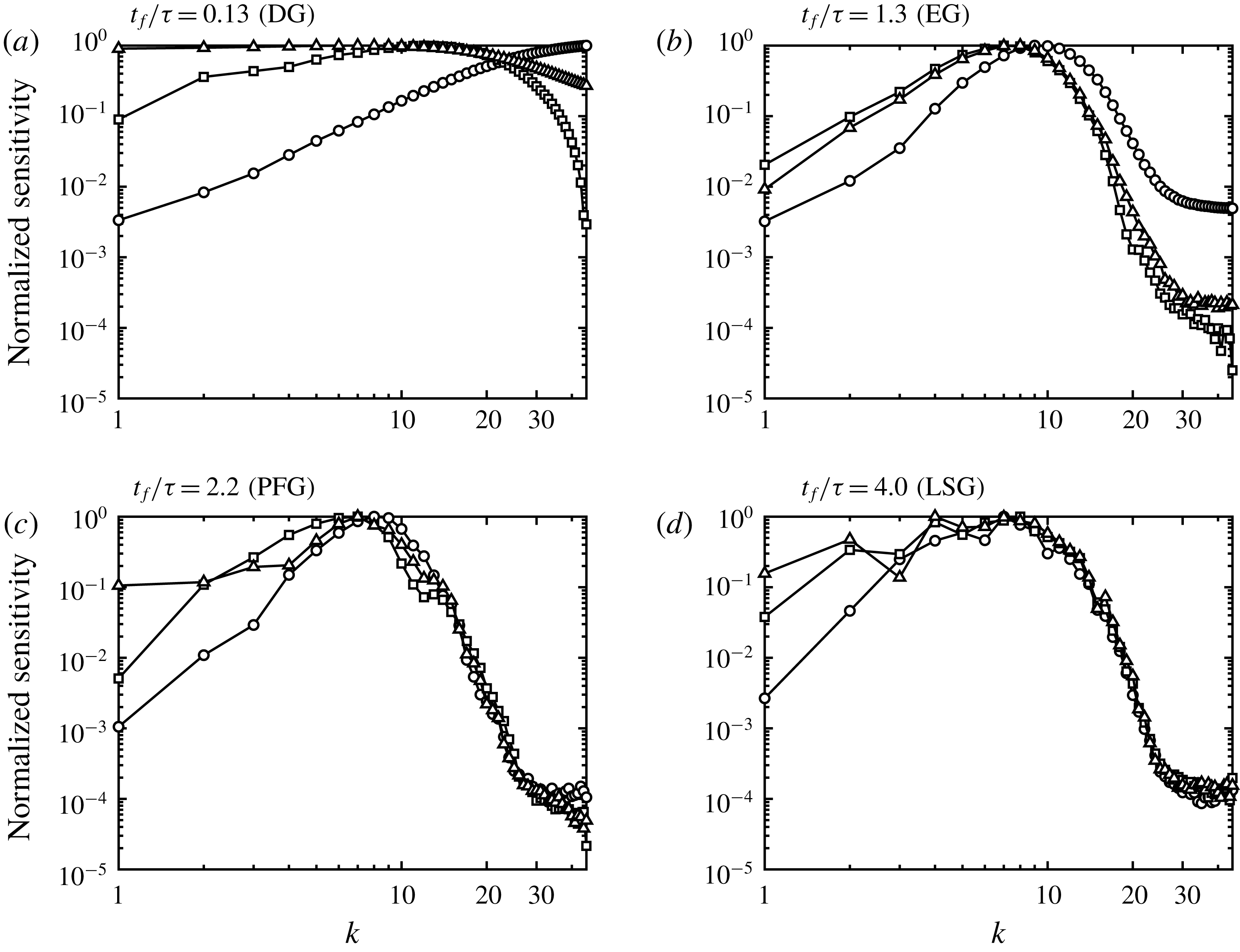
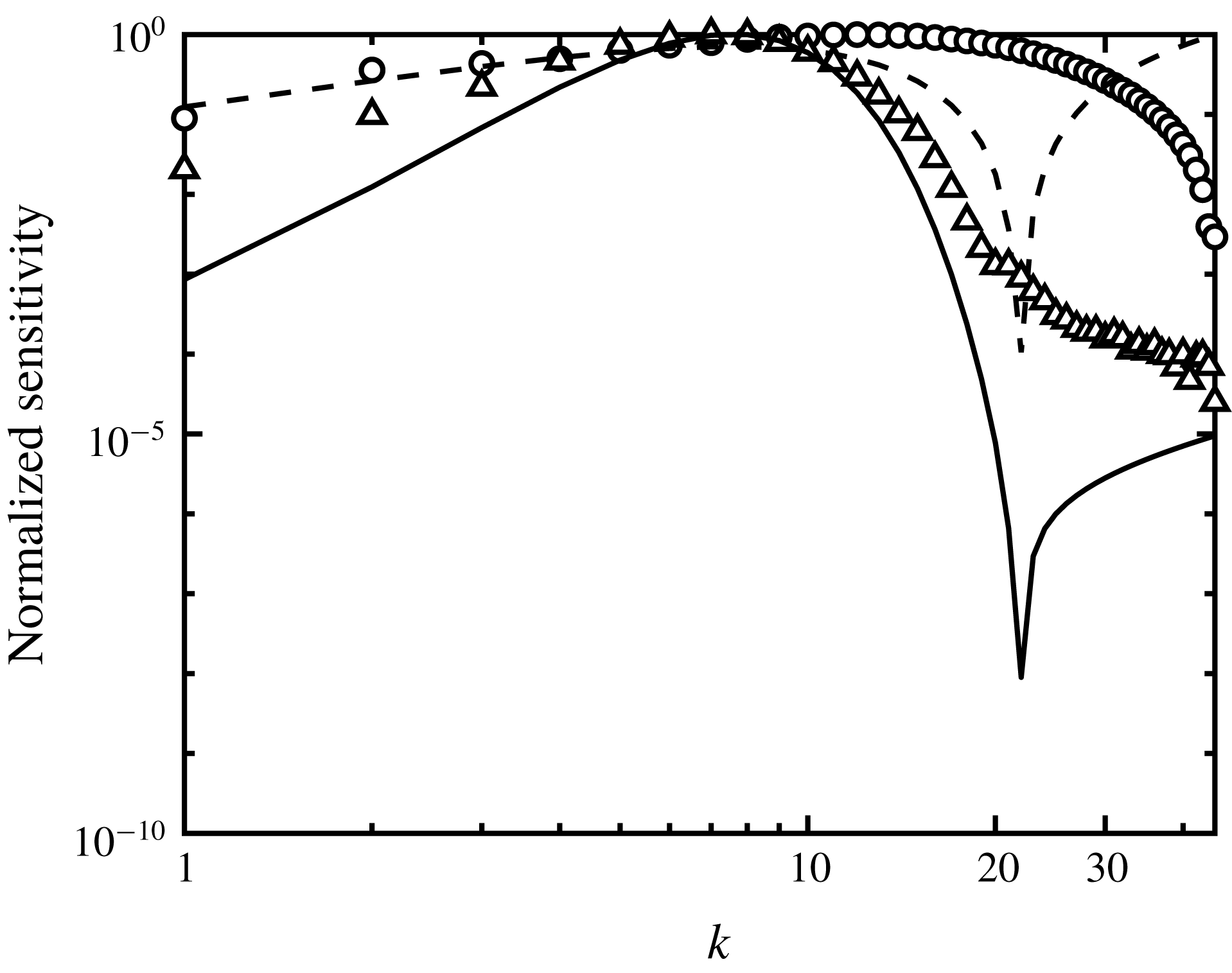
Magnitude of sensitivity $|\unicode[STIX]{x1D6FF}{\mathcal{J}}/\unicode[STIX]{x1D6FF}\boldsymbol{A}|$ integrated over different durations $t_{f}$ for $\text{MIX}$ (–○–), $\text{KE}$ (–▫–) and $\text{VAR}$ (–▵–). The sensitivities are shown as a function of initial perturbation wavenumber $k=\sqrt{k_{x}^{2}+k_{z}^{2}}$ and normalized by their corresponding maximum value.

4.2 Sensitivities to different measures of mixing

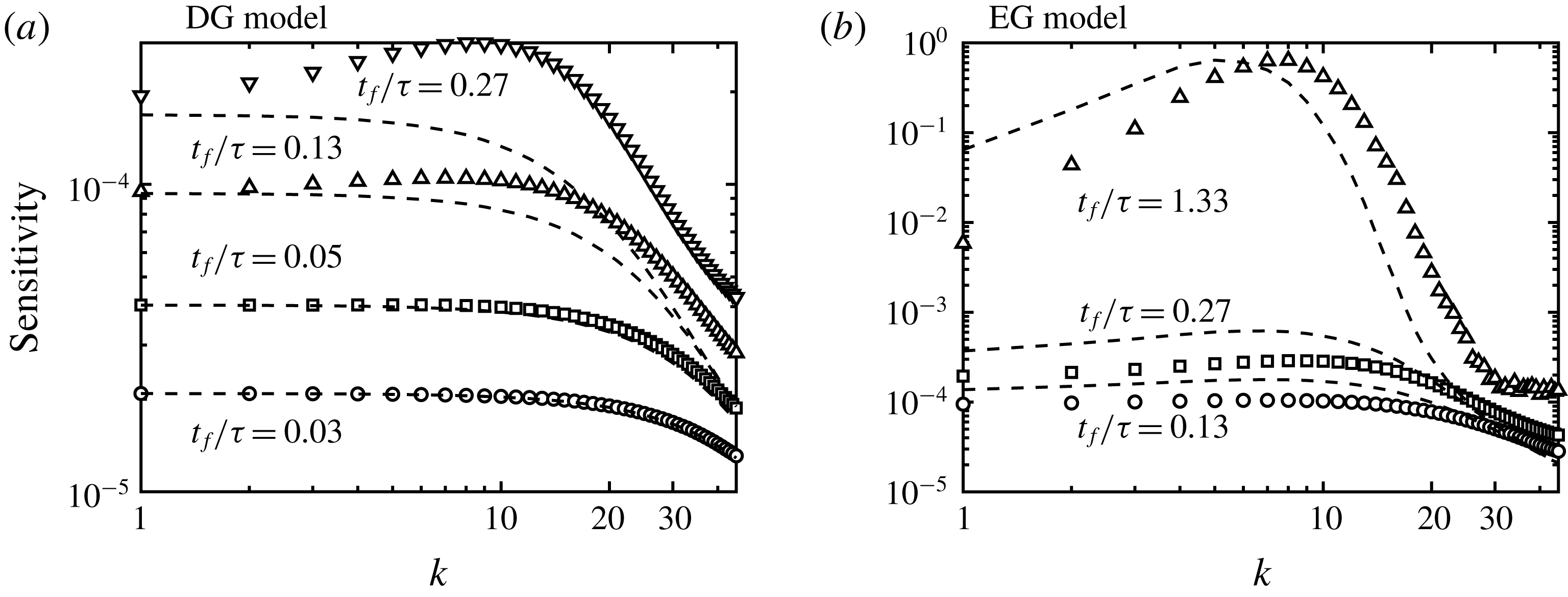
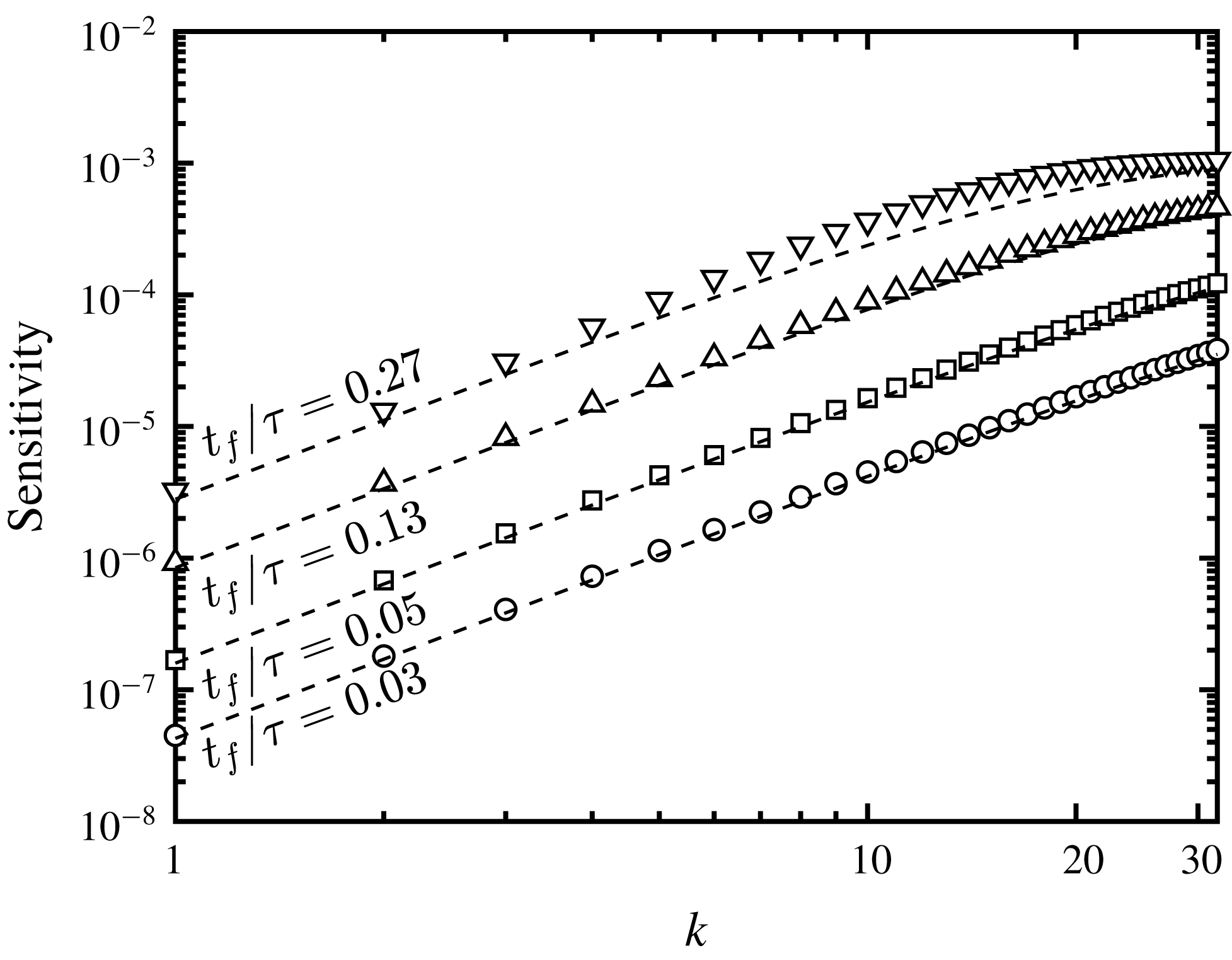
The sensitivity of ${\mathcal{J}}$ to $\boldsymbol{A}$ over duration $t_{f}$ are evaluated across the averaged perturbation wavenumbers $k=\sqrt{k_{x}^{2}+k_{z}^{2}}$ (see figure 4). It can immediately be seen that at early stages of the RT instability the distribution of sensitivity varies between the different quantities of interest, and collapse at late time. Within the DG stage, $\text{VAR}$ and $\text{KE}$ are most sensitive to low and intermediate wavenumber perturbations, and are least sensitive at the highest wavenumbers (see figure 4 a). Perhaps surprisingly, $\text{MIX}$ exhibits an opposite trend, with sensitivity increasing with increasing $k$ . This suggests that when diffusion dominates, the largest changes to the quantity $X(1-X)$ can be achieved by perturbing the perturbation amplitude at the highest wavenumbers. This early-time behaviour can be predicted analytically by assuming the mole fraction evolves according to a diffusion equation. 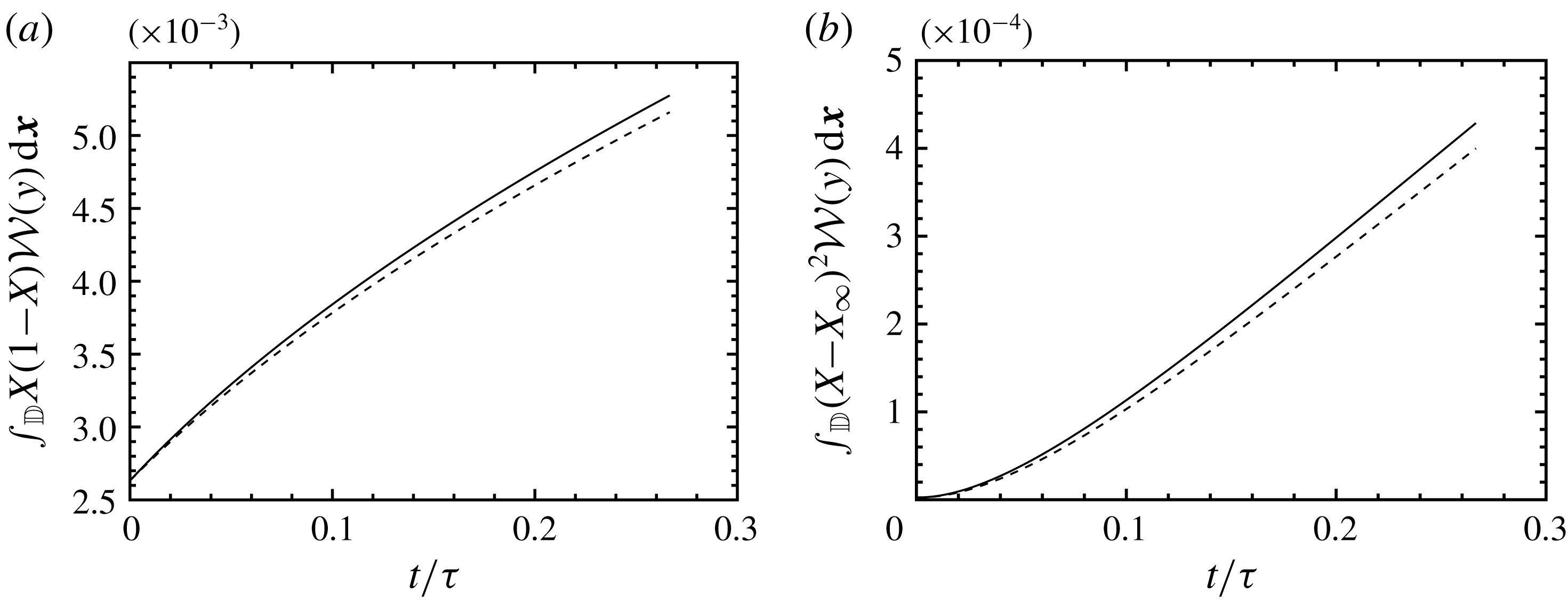Assuming purely diffusional growth, the distribution of sensitivity with $k$ can be shown to be a consequence of the functional dependence of ${\mathcal{J}}$ on $X$ and initial conditions. A detailed comparison of the theoretical estimates of early-time sensitivity and the adjoint solution for each objective function is provided in appendix B.

Inertial effects from buoyancy become more significant as time increases. Linear stability theory predicts that the exponential growth rate within the EG regime, $\unicode[STIX]{x1D70E}_{k}^{(EG)}$ , is given by (Duff et al. Reference Duff, Harlow and Hirt1962)

(4.1) $$\begin{eqnarray}\displaystyle \unicode[STIX]{x1D70E}_{k}^{(EG)}=\left[\frac{At\,k}{\unicode[STIX]{x1D713}Fr_{c}}+\frac{k^{4}}{\unicode[STIX]{x1D70C}_{I}^{2}Re_{c}^{2}}\right]^{1/2}-\left(1+Sc^{-1}\right)\frac{k^{2}}{\unicode[STIX]{x1D70C}_{I}Re_{c}}, & & \displaystyle\end{eqnarray}$$

where $\unicode[STIX]{x1D713}$ depends on the Atwood number, wavenumber and the thickness of the diffusive layer (see Duff et al. Reference Duff, Harlow and Hirt1962). The above relation predicts $k=7.58$ as the most unstable wavenumber at $t=0$ . As shown in figure 4(b), this is consistent with the most sensitive wavenumber provided by the adjoint solution in the EG regime. As the time duration increases, the most sensitive modes corresponding to $\text{MIX}$ shifts from the highest wavenumbers to lower ones. Within the PFG and LSG regimes, the distribution of sensitivity is similar for all objective functions, with maximum sensitivity remaining close to the most unstable wavenumber predicted by linear stability theory. Except for $\text{MIX}$ in the DG regime, the objective functions are generally unaffected by perturbation modes at wavenumbers $k>20$ . Linear stability theory predicts that these modes are damped by diffusion during the EG regime.

It is interesting to note that the most sensitive wavenumber throughout the growth of the RT instability remains approximately constant and consistent with the most unstable wavenumber predicted by linear stability theory. However, its distribution varies. This suggests that employing linear stability theory for manipulating growth of the instability may have only limited success due to the broadband nature of sensitivity. This will be confirmed in § 5.

It is important to note that the sensitivity obtained by the adjoint solution in chaotic dynamic systems is known to diverge when measured over long time horizons (e.g. see Lea et al. Reference Lea, Allen and Haine2000; Wang & Gao Reference Wang and Gao2013). Thus, the values used for normalization in figure 4 will change depending on the duration considered. Following Wang & Gao (Reference Wang and Gao2013), its chaotic behaviour is characterized by estimating the first Lyapunov exponent, $\unicode[STIX]{x1D6EC}$ , for the adjoint solution of each objective function over the duration $t_{f}=4.0\unicode[STIX]{x1D70F}$ , according to

(4.2) $$\begin{eqnarray}\displaystyle \mathop{\left\Vert \mathop{\sum }_{i=1}^{6}Q_{i}^{\dagger }(\boldsymbol{x},t){\mathcal{W}}_{\unicode[STIX]{x1D6E4}}(y)\right\Vert }\nolimits_{2}\propto \exp (-\unicode[STIX]{x1D6EC}t), & & \displaystyle\end{eqnarray}$$

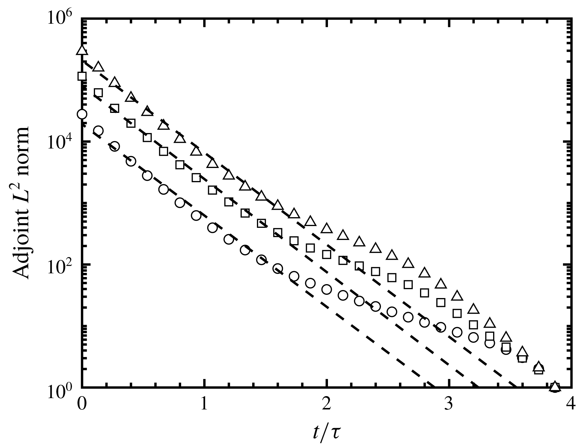
where $\Vert \cdot \Vert _{2}$ is a spatial $L^{2}$ norm operator, and $i=1,\ldots ,6$ denotes the $i$ th component of adjoint variable. The value of $\unicode[STIX]{x1D6EC}$ estimates the average growth rate in $\unicode[STIX]{x1D6FF}{\mathcal{J}}$ due to small changes in initial interfacial perturbations (e.g. see Trevisan & Legnani Reference Trevisan and Legnani1995). As can be seen in figure 5, the magnitude of the adjoint variables exponentially increase in inverse time with rates $\unicode[STIX]{x1D6EC}=3.42\unicode[STIX]{x1D70F}^{-1}$ , $3.48\unicode[STIX]{x1D70F}^{-1}$ and $3.45\unicode[STIX]{x1D70F}^{-1}$ for $\text{MIX}$ , $\text{KE}$ and $\text{VAR}$ , respectively. From this, the rate at which sensitivity diverges does not significantly differ among the different objective functions. We note that the positive first Lyapunov exponents of each objective function limits the time horizon that can be considered, which may affect the optimization of the instability during late-time growth. The utility of the adjoint solution for controlling the RT instability will be addressed in § 5.3. The next section will analyse local sensitivity at various stages of the instability.

Figure 5.

The $L^{2}$ norm of adjoint solutions for $\text{MIX}$ (○), $\text{KE}$ (▫) and $\text{VAR}$ (▵). The $L^{2}$ norms are normalized by the corresponding values at $t=3.87\unicode[STIX]{x1D70F}$ . The dashed lines estimate the growth in the adjoint solution based on the first Lyapunov exponent, which was found to be $\unicode[STIX]{x1D6EC}=3.42\unicode[STIX]{x1D70F}^{-1}$ , $3.48\unicode[STIX]{x1D70F}^{-1}$ and $3.45\unicode[STIX]{x1D70F}^{-1}$ for $\text{MIX}$ , $\text{KE}$ and $\text{VAR}$ , respectively.

4.3 Spatial sensitivity at various stages of the RT instability

In this section we evaluate the spatial distribution of sensitivity at different stages of the instability. The sensitivity gradient defined in (3.16) can be rewritten as

(4.3) $$\begin{eqnarray}\displaystyle \frac{\unicode[STIX]{x1D6FF}{\mathcal{J}}}{\unicode[STIX]{x1D6FF}\boldsymbol{Q}_{0}}=\int _{\mathbb{D}}\int _{0}^{t_{f}}\frac{\unicode[STIX]{x1D6FF}{\mathcal{I}}}{\unicode[STIX]{x1D6FF}\boldsymbol{Q}_{0}}\,\text{d}t\,\text{d}\boldsymbol{x}=\int _{\mathbb{D}}\boldsymbol{Q}_{0}^{\dagger }\,\text{d}\boldsymbol{x}. & & \displaystyle\end{eqnarray}$$

Thus, the local adjoint variables $Q_{i}^{\dagger }$ at $t=0$ provide spatial sensitivity of the mixing norms to the flow state. With this, the local sensitivity of ${\mathcal{J}}$ with respect to initial mole fraction variations can be expressed as

(4.4) $$\begin{eqnarray}\frac{\unicode[STIX]{x1D6FF}{\mathcal{J}}}{\unicode[STIX]{x1D6FF}X_{0}}=\unicode[STIX]{x1D70C}Y^{\dagger }\frac{\unicode[STIX]{x2202}Y}{\unicode[STIX]{x2202}X},\end{eqnarray}$$

where the chain rule is used, and $\unicode[STIX]{x2202}Y/\unicode[STIX]{x2202}X$ can be determined using the relation $Y=XW_{1}/W$ .

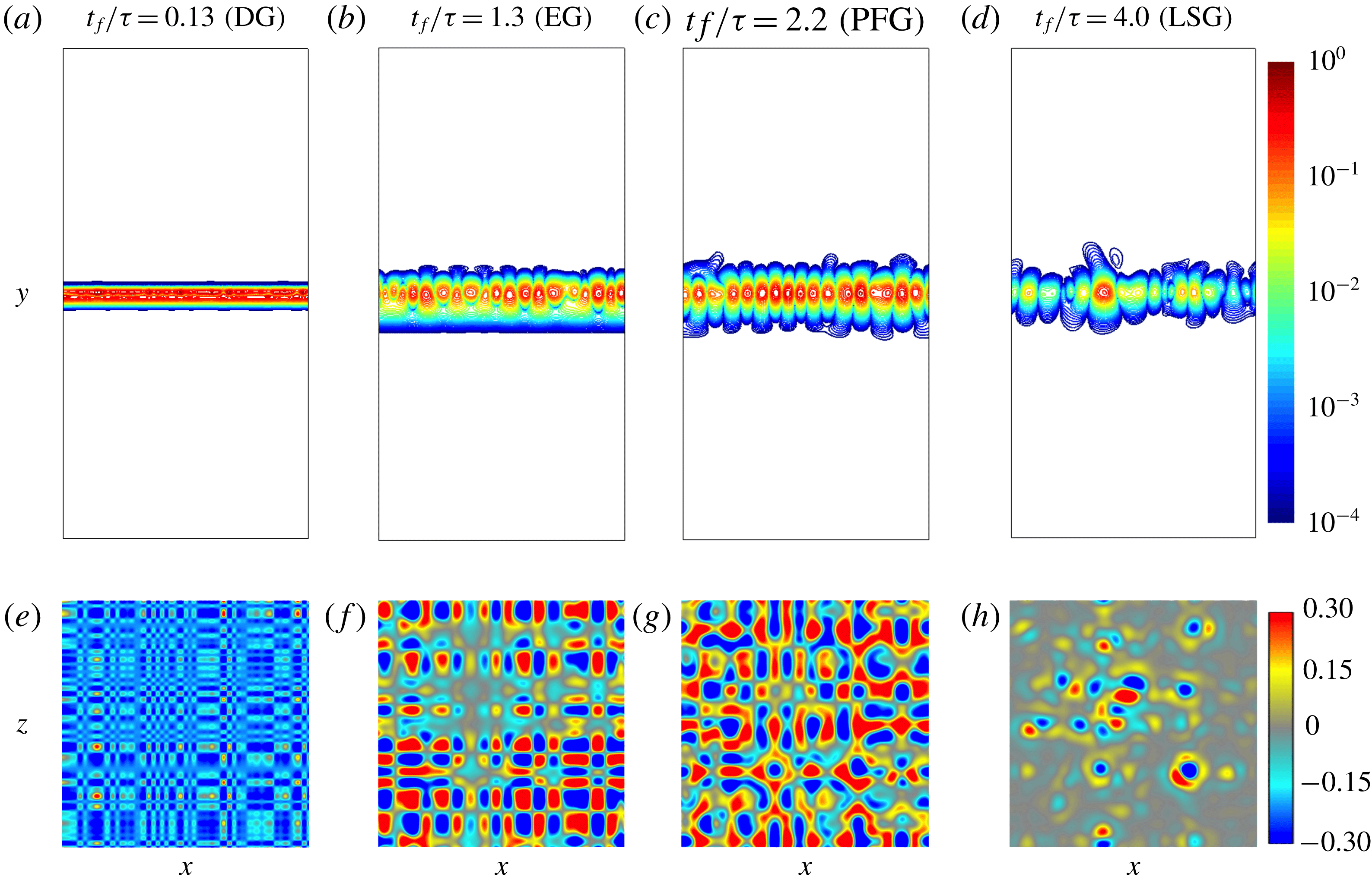
The spatial distribution of $\unicode[STIX]{x1D6FF}{\mathcal{J}}/\unicode[STIX]{x1D6FF}X_{0}$ for $\text{VAR}$ integrated over different durations in the vertical plane $z=-\unicode[STIX]{x03C0}$ are compared in figures 6(a)–6(d) and at the fluid interface $X=0.5$ in figures 6(e)–6(h). As can be seen in figures 6(a)–6(d), local sensitivity exhibits a periodic distribution that is maximum near the interface. As was shown in the previous section, the dominant wavenumber of local sensitivity at the interface during the EG stage corresponds to $k\simeq 7$ , consistent with the most unstable wavenumber mode predicted by liner stability theory (see figure 6 f). Local sensitivity does not significantly change from EG to PFG (see figure 6 g). However, the sensitivity in the LSG stage exhibits more variations near the interface, suggesting a broader range of modes contribute to mixing. Figures 6(e)–6(h) show that adjusting the perturbations at the fluid interface could both locally increase (positive sensitivity) or decrease (negative sensitivity) the mixing norm. Non-uniformities in sensitivity observed at the $x$ – $z$ plane suggest that the effects of spatial variations in the initial conditions on mixing persist at late time stages of the growth.

Figure 6.

Normalized sensitivities of $\text{VAR}$ to initial mole fraction ( $\unicode[STIX]{x1D6FF}{\mathcal{J}}/\unicode[STIX]{x1D6FF}X_{0}$ ) in physical space for different time durations $t\in [0,t_{f}]$ . The sensitivities are normalized by their maximum value. (a–d) Normalized sensitivity magnitude at $z=-\unicode[STIX]{x03C0}$ . (e–h) Normalized sensitivity at the fluid interface ( $X=0.5$ ).

4.4 The role of initial conditions on late-time sensitivity

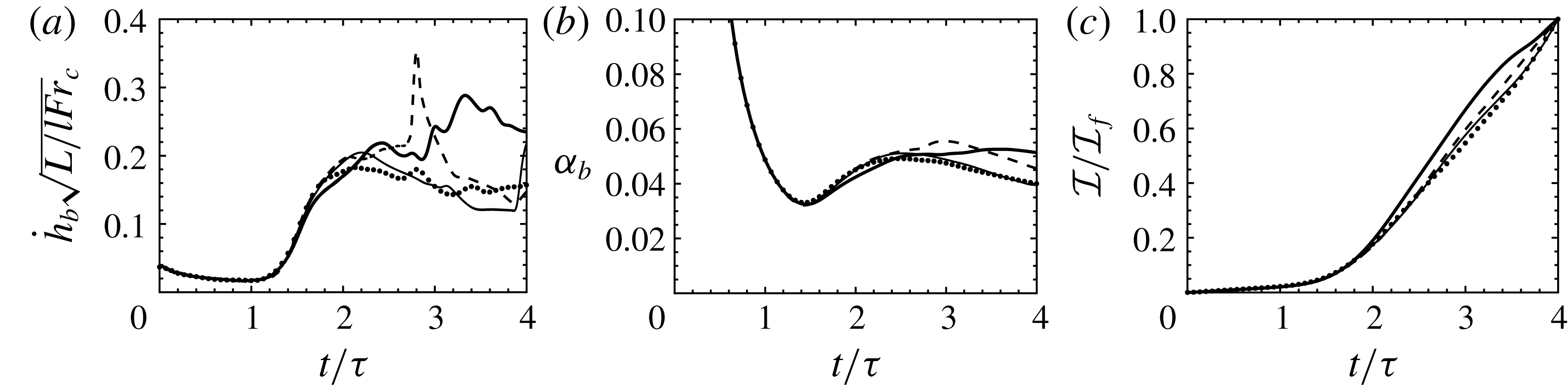
In the previous sections we considered initial interfacial perturbations with uniform amplitude and random phase. In order to evaluate the effects of initial perturbations on different stages of the RT growth, phases $\unicode[STIX]{x1D703}_{x,m}$ and $\unicode[STIX]{x1D703}_{z,n}$ are varied while holding the amplitudes constant. Haan (Reference Haan1989) showed that a group of perturbation modes with similar phases can regionally combine and create a net perturbation amplitude during an RT instability. Thus, we expect that changing the initial perturbation phases while holding the initial amplitudes constant should lead to different nonlinear growth. The evolution of ${\dot{h}}_{b}$ , $\unicode[STIX]{x1D6FC}_{b}$ and ${\mathcal{I}}=(X-X_{\infty })^{2}$ with different initial random phases are compared in figure 7. The bubble growth during the DG and EG stages is insensitive to the initial random phases, while deviations appear during the PFG and LSG regimes (see figure 7 a). The bubble tip velocity corresponding to one of the realization decelerates following a PFG state, and later reaccelerates. On the other hand, another realization exhibits a reacceleration regime after PFG, prior to deceleration. Another realization exhibits a long PFG regime, with a slight deceleration in the bubble growth rate $\unicode[STIX]{x1D6FC}_{b}$ while the other illustrates a combination of short-time accelerations and decelerations during the LSG regime. A chaotic behaviour is observed during the LSG regime. Meanwhile, it can be seen that the bubble growth parameter $\unicode[STIX]{x1D6FC}_{b}$ marginally changes for these initial conditions (see figure 7 b). In addition, the objective function ${\mathcal{I}}=(X-X_{\infty })^{2}$ corresponding to different initial phases is similar until $t\approx 2\unicode[STIX]{x1D70F}$ at which point it diverges (see figure 7 c).

Figure 7.

Evolution of (a) the bubble tip velocity, (b) bubble growth parameter and (c) instantaneous objective function $\text{VAR}$ ( ${\mathcal{I}}=(X-X_{\infty })^{2}$ ), for four different initial interfacial perturbations of the three-dimensional RT instability.

Figure 8.

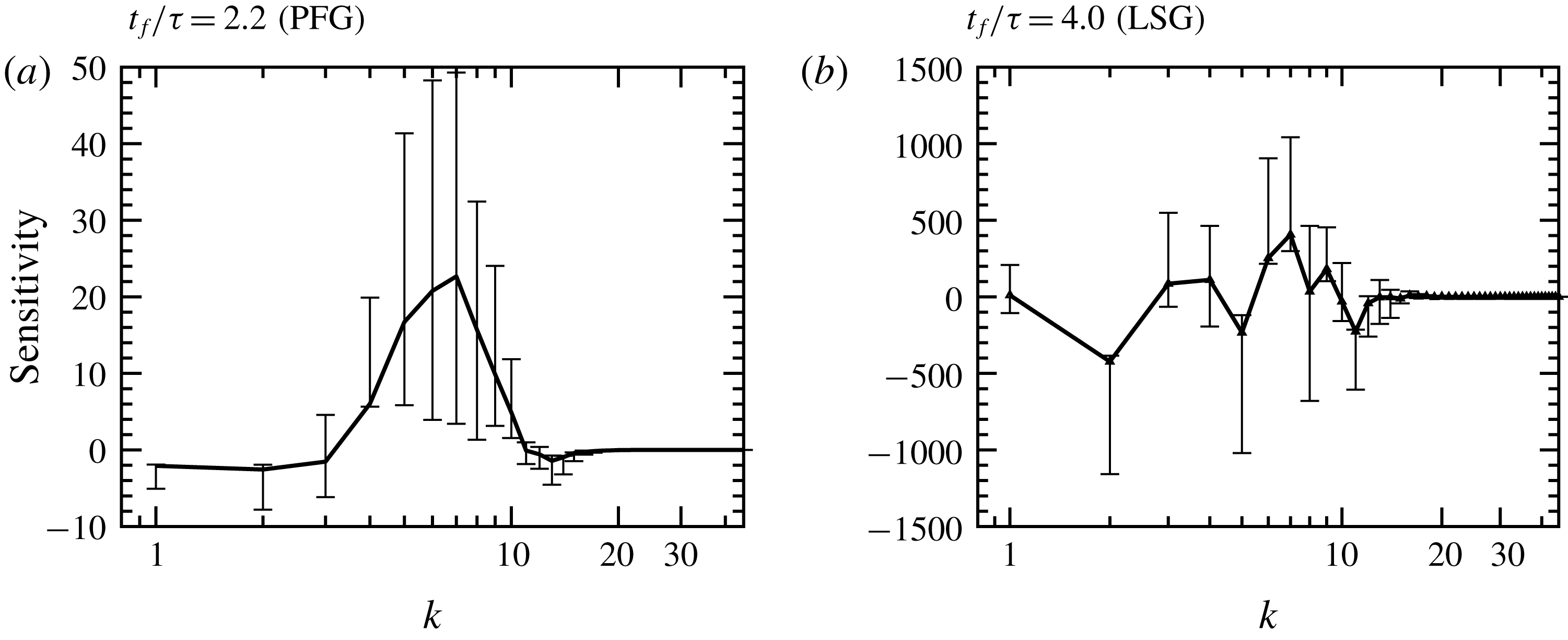
Ensemble-averaged sensitivities of $\text{VAR}$ ( $\unicode[STIX]{x1D6FF}{\mathcal{J}}/\unicode[STIX]{x1D6FF}\boldsymbol{A}$ ) for different random initial phases. The sensitivities are shown as a function of initial perturbation wavenumber $k=\sqrt{k_{x}^{2}+k_{z}^{2}}$ . The vertical bars illustrate the minimum and maximum sensitivities at each wavenumber.

Figure 7 shows that the growth is insensitive to initial random phases until $t\approx 2\unicode[STIX]{x1D70F}$ . For each $k$ , the sensitivity averaged over all realizations during early ( $t_{f}=2.2\unicode[STIX]{x1D70F}$ ) and late ( $t_{f}=4.0\unicode[STIX]{x1D70F}$ ) nonlinear stages is shown in figure 8. It can be seen that randomly adjusting the phases leads to significant variations in sensitivity at late stages. A set of modes $2\leqslant k\leqslant 10$ is highly sensitive to initial phases when $t_{f}=2.2\unicode[STIX]{x1D70F}$ (see figure 8 a). At later times, a broader range of modes are sensitive to the initial phases (see figure 8 b). This is consistent with the positive values of the first Lyapunov exponent discussed in § 4.2 (see figure 5).

5.1 Selectively assigning the perturbation energy

Before performing the optimization, two-dimensional simulations of RT instabilities are reported with carefully chosen interfacial perturbations for comparison in later sections. As discussed in § 4, perturbations with wavenumbers $k>21$ are suppressed during the EG stage according to linear stability theory (Duff et al. Reference Duff, Harlow and Hirt1962). Therefore, it is expected that the optimized solution for minimizing RT mixing corresponds to an interface with all of the energy contained in the highest wavenumbers, leading to pure diffusional growth. Yet, the optimized solution for enhancing mixing is less obvious. In the context of scalar mixing, it is well known that large flow structures are controlled by advection while small length scales are mainly mixed by diffusion (e.g. see Foures et al. Reference Foures, Caulfield and Schmid2014; Miles Reference Miles2018). For RT instabilities, it has been observed that assigning more perturbation energy into low wavenumber modes increases the growth parameter $\unicode[STIX]{x1D6FC}$  (e.g. see Cook & Dimotakis Reference Cook and Dimotakis2001; Ristorcelli & Clark Reference Ristorcelli and Clark2004; Banerjee & Andrews Reference Banerjee and Andrews2009; Youngs Reference Youngs2009). In addition, Cook & Dimotakis (Reference Cook and Dimotakis2001) showed that seeding the lowest wavenumbers leads to ‘the largest unmixedness’. In summary, it is expected that increased bubble/spike penetration occurs when more perturbation energy is added to low wavenumbers of the initial interface. When the perturbations are distributed among the highest wavenumber modes mixing is dominated by diffusion.

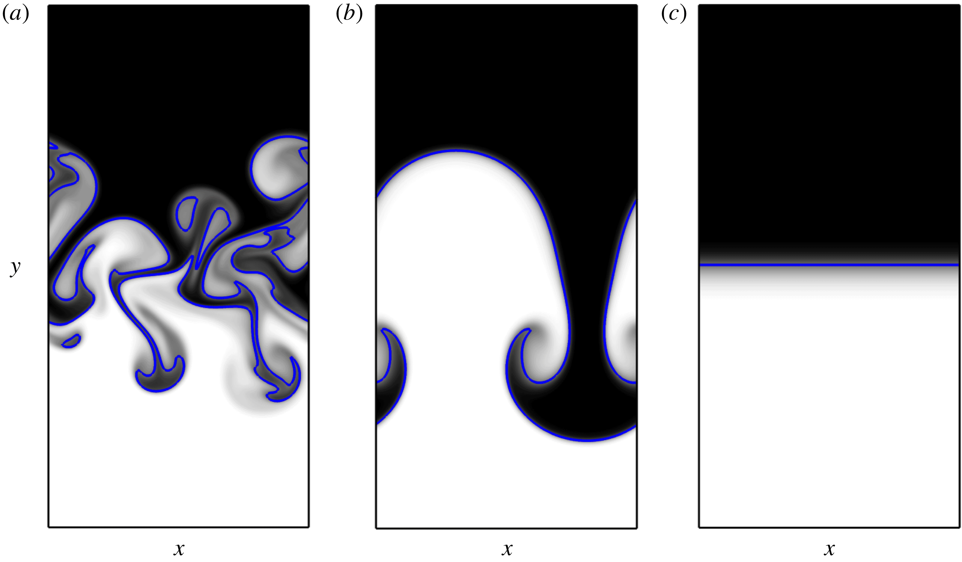
With this in mind, three different initial conditions are considered: (i) a uniform distribution of modal energy with random phases (similar to the configuration used § 4) serving as the baseline solution for the remainder of the paper; (ii) all the energy contained in the lowest wavenumber denoted here as Case A; and (iii) all the energy contained in the highest wavenumber referred to here as Case B. As shown in figure 9, the baseline case yields bubble and spike penetration associated with low perturbation wavenumbers as well as diffusion mixing associated with high wavenumbers. Nonlinear mode coupling also occurs due to the existence of high wavenumber interfacial perturbations. Case A produces large amounts of penetration through the formation of a bubble and spike. The interfacial perturbation is suppressed in Case B during early-time regimes according to linear stability theory (Duff et al. Reference Duff, Harlow and Hirt1962), and mixing is dominated by diffusion throughout the duration of the simulation.

Figure 9.

Bubble and spike structures of a two-dimensional RT instability at $t=4.0\unicode[STIX]{x1D70F}$ with different initial interfacial perturbations. (a) Baseline (uniform amplitude among all wavenumbers), (b) Case A (all energy contained in the lowest mode) and (c) Case B (all energy contained in the largest mode). Same colour scheme as figure 2.

Values of the corresponding objective functions for the three cases are reported in table 1. Both the lowest and highest wavenumber distributions produce smaller $\text{MIX}$  values compared to the uniform distribution. The corresponding integrand, ${\mathcal{I}}=X(1-X)$ , is maximum for completely mixed fluid ( $X=0.5$ ) and zero for pure fluids. Thus, neither single-mode case produces as much mixing as in the uniform case as a result of nonlinear mode coupling. Case A demonstrates solely large-scale fluid penetration, resulting in high interfacial velocity and thus larger values of $\text{KE}$ compared the other objective functions. Assigning the initial perturbation energy into the lowest mode increases $\text{KE}$ by almost a factor of 2 compared to the baseline case. Comparatively, putting all the perturbation energy into the highest wavenumber decreases $\text{KE}$ by 5 orders of magnitude due to dissipation of kinetic energy by diffusion. Putting all the energy into the lowest mode increases $\text{VAR}$ by almost 30 % compared to the baseline case. The largest possible value of the $\text{VAR}$ integrand, ${\mathcal{I}}_{\infty }=(X-X_{\infty })^{2}$ , occurs when the two fluids are inverted (i.e. the light fluid on top and heavy fluid on bottom). Thus, larger values of $\text{VAR}$ occur in the presence of fluid penetration rather than pure mixing.

Table 1.

Objective functions measured over duration $t_{f}=4.0\unicode[STIX]{x1D70F}$ normalized by their baseline solution ${\mathcal{J}}^{(0)}$ (uniformly distributed perturbation energy).

Figure 10.

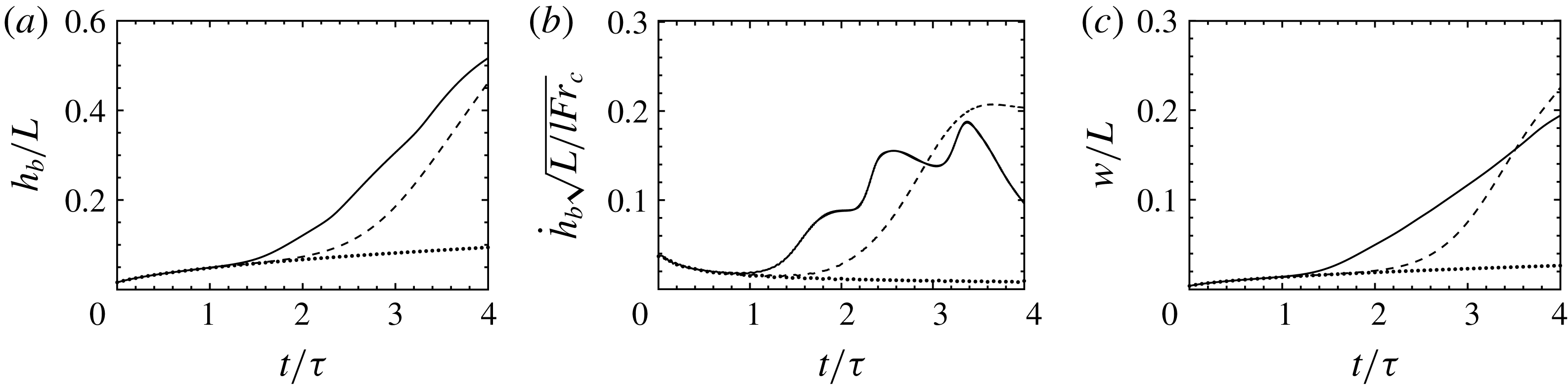
Evolution of (a) bubble height, (b) bubble tip velocity and (c) mixing width of the two-dimensional RT instability with different initial interfacial perturbation energy: baseline (–), Case A (– –) and Case B $(\cdots \,)$ .

Figure 10 shows a comparison of the bubble height, bubble tip velocity and mixing width of the two-dimensional RT instability with the three different initial conditions. The bubble tip velocity in Case A approaches the PG regime at a later time compared to the baseline case due to the baseline case containing energy in modes with greater exponential growth rate. In addition, nonlinear mode-coupling effects absent in Case A and Case B result in increased growth. The EG stage holds while $h_{0}\ll \unicode[STIX]{x1D706}$ , and thus Case A will not exceed the EG regime until a greater time interval has passed compared with the baseline case. In contrast, the bubble tip velocity of Case B decreases due to diffusion.

Finally, it can be seen that the two-dimensional multi-mode RT instability (figures 9 and 10) grows more slowly compared to the three-dimensional flow (figures 1 and 2). This is consistent with previous work that shows how three-dimensional RT instabilities grow faster than their two-dimensional counterparts during the early nonlinear regime (Layzer Reference Layzer1955; Hecht et al. Reference Hecht, Alon and Shvarts1994; Oron et al. Reference Oron, Arazi, Kartoon, Rikanati, Alon and Shvarts2001; Goncharov Reference Goncharov2002). This is due to reduced kinematic drag associated with three-dimensional bubbles compared to elongated two-dimensional bubbles, leading to a greater terminal bubble tip velocity in three dimensions.

Figure 11.

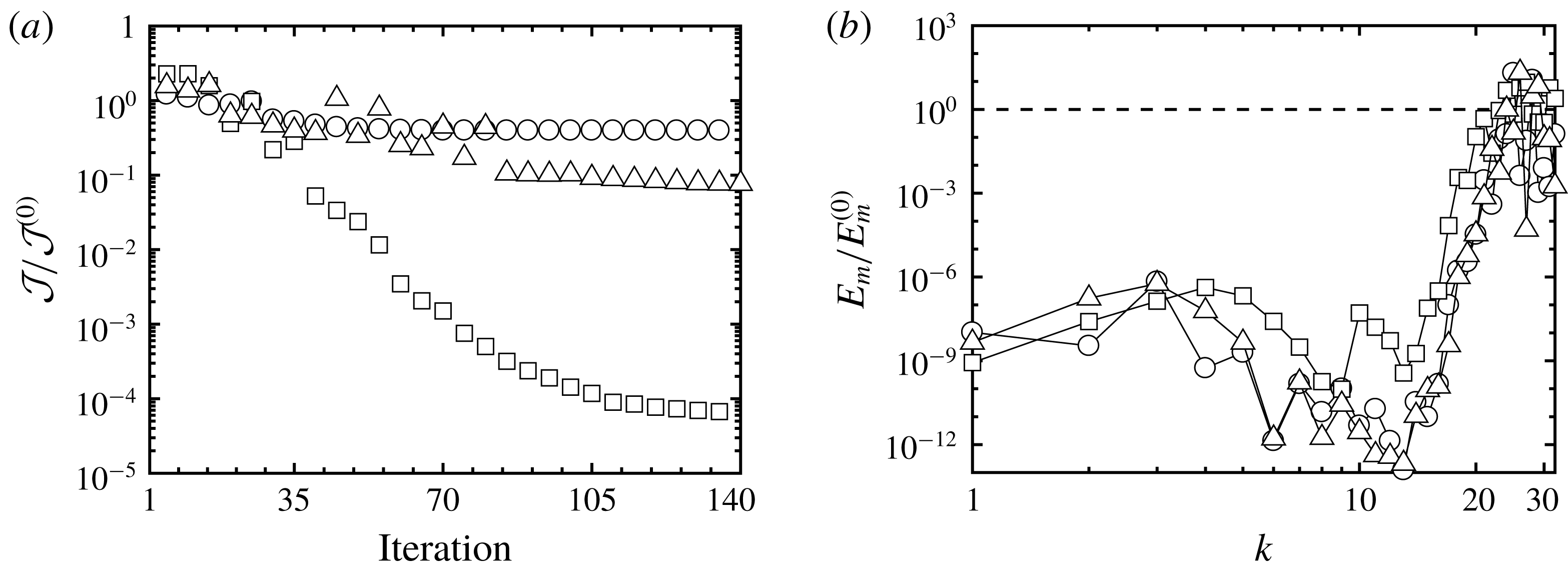
(a) Reduction of the objective functions normalized by their corresponding baseline values ${\mathcal{J}}^{(0)}$ for $\text{MIX}$ (○), $\text{KE}$ (▫) and $\text{VAR}$ (▵). (b) The spectrum of interfacial perturbation energy for the baseline case (– –) and the optimized solution (symbols).

5.2 Optimal solution for suppressing mixing

As discussed in the previous section, we expect mixing and growth to be suppressed by transferring all of the perturbation energy into the highest wavenumber modes such that diffusion dominates. In this section, this solution is sought by minimizing the objective functions via the gradient-based optimization method described earlier. Figure 11(a) shows the value of each objective function during the iterative process of the optimization procedure. Different levels of reduction are observed for each objective function. The optimized quantities are listed in table 1. Adjoint-based optimization is capable of reducing $\text{KE}$ and $\text{VAR}$ by more than an order of magnitude compared to their baseline values while $\text{MIX}$ is only reduced by approximately 60 %. Due to the initially smooth distribution of mole fraction as defined in (2.12), $\text{MIX}$ will remain finite even in the absence of any mixing or growth. As a consequence, its optimal solution approaches the value from Case B and not zero. As expected, the perturbation energy of the optimized solution for each objective function is transferred to high wavenumber modes, resulting in diffusion dominated growth (see figure 11 b).

5.3 Optimal solution for enhancing mixing

Based on previous studies of multi-mode RT instabilities (e.g. see Cook & Dimotakis Reference Cook and Dimotakis2001; Ristorcelli & Clark Reference Ristorcelli and Clark2004; Banerjee & Andrews Reference Banerjee and Andrews2009; Youngs Reference Youngs2009), it is anticipated that maximizing late-time growth requires shifting the perturbation energy towards the low wavenumber modes. In this section, we seek the optimal distribution of modal energy that enhances the three objective functions with respect to the baseline case denoted by ${\mathcal{J}}^{(0)}$ – an interface with uniform amplitude and random phase. It should be noted that gradient-based optimization provides a local extremum and there is no guarantee that such a solution holds globally. To this end, different initial configurations were considered as the starting point in the optimization process. The optimized spectra reported here correspond to an initial distribution of modal energy that was found to produce the greatest changes in ${\mathcal{J}}$ .

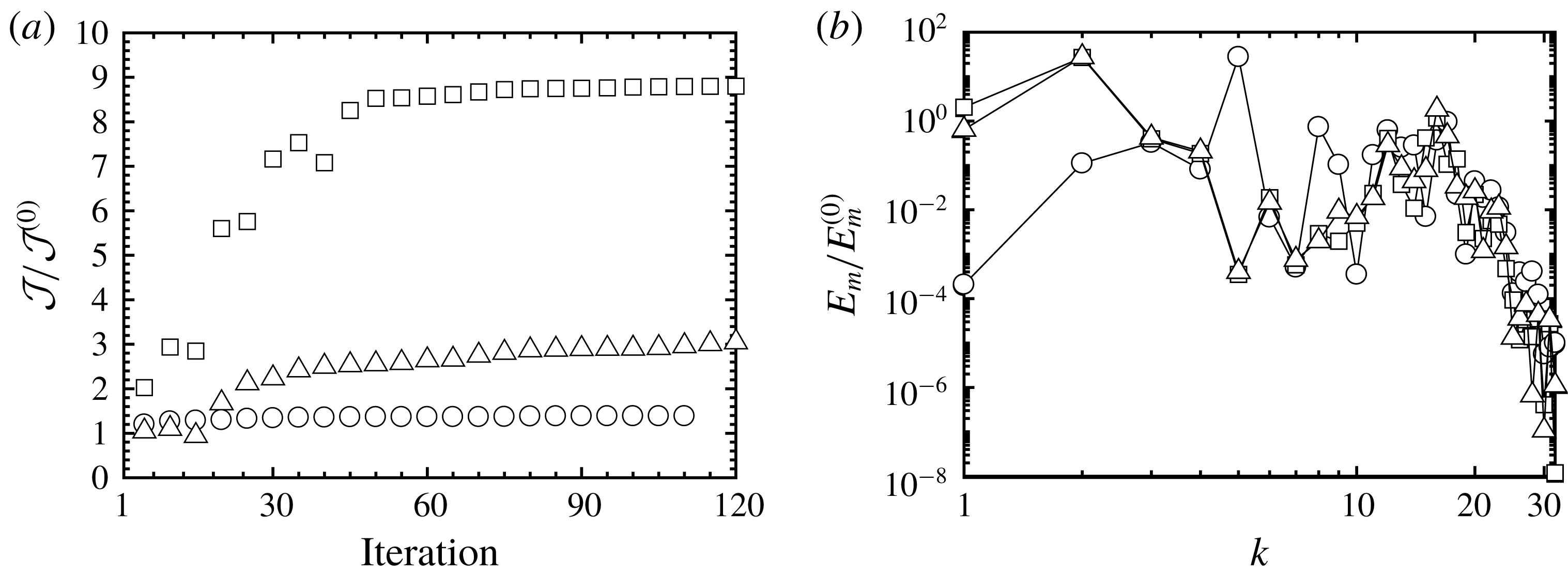
The iteration history of the three objective functions shows that $\text{MIX}$ is increased by approximately 40 %, $\text{KE}$ by 900 % and $\text{VAR}$ by 300 % (see table 1 and figure 12 a). The initial interfacial perturbation energy of the three enhanced solutions indicates that low wavenumber modes have a greater contribution to RT growth and mixing (see figure 12 b). It can be seen that the majority of perturbation energy of the high wavenumber modes is transferred to the first five wavenumbers. The optimized solutions exhibit non-trivial mode competition and coupling effects that enhance mixing. Nonlinear mode coupling generates lower wavenumber modes that move faster in the flow during the potential regime. Mode coupling also creates high wavenumber modes that are diminished by molecular diffusion. These effects are reflected in the optimized initial perturbations shown in figure 12(b), especially for the objective functions that measure the fluid penetration and growth, i.e. $\text{KE}$ and $\text{VAR}$ . It can be seen that the perturbation energy sharply decreased for $k>21$ , where the exponential growth rate is expected to be negative according to linear stability theory.

Figure 12.

(a) Enhancement of the objective functions over duration $t_{f}=4\unicode[STIX]{x1D70F}$ normalized by their corresponding baseline values ${\mathcal{J}}^{(0)}$ for $\text{MIX}$ (○), $\text{KE}$ (▫), and $\text{VAR}$ (▵). (b) The spectrum of initial interfacial perturbation energy of the optimized solution.

Figure 13.

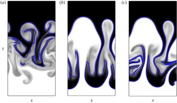
Mole fraction at $t=4.0\unicode[STIX]{x1D70F}$ of the optimized solution for enhancing the three objective functions (a) $\text{MIX}$ , (b) $\text{KE}$ and (c) $\text{VAR}$ . Compared to the baseline case, $\text{MIX}$ , $\text{KE}$ and $\text{VAR}$ are enhanced by factors of $1.4$ , $8.9$ and $3.1$ , respectively. Same colour scheme as figure 2.

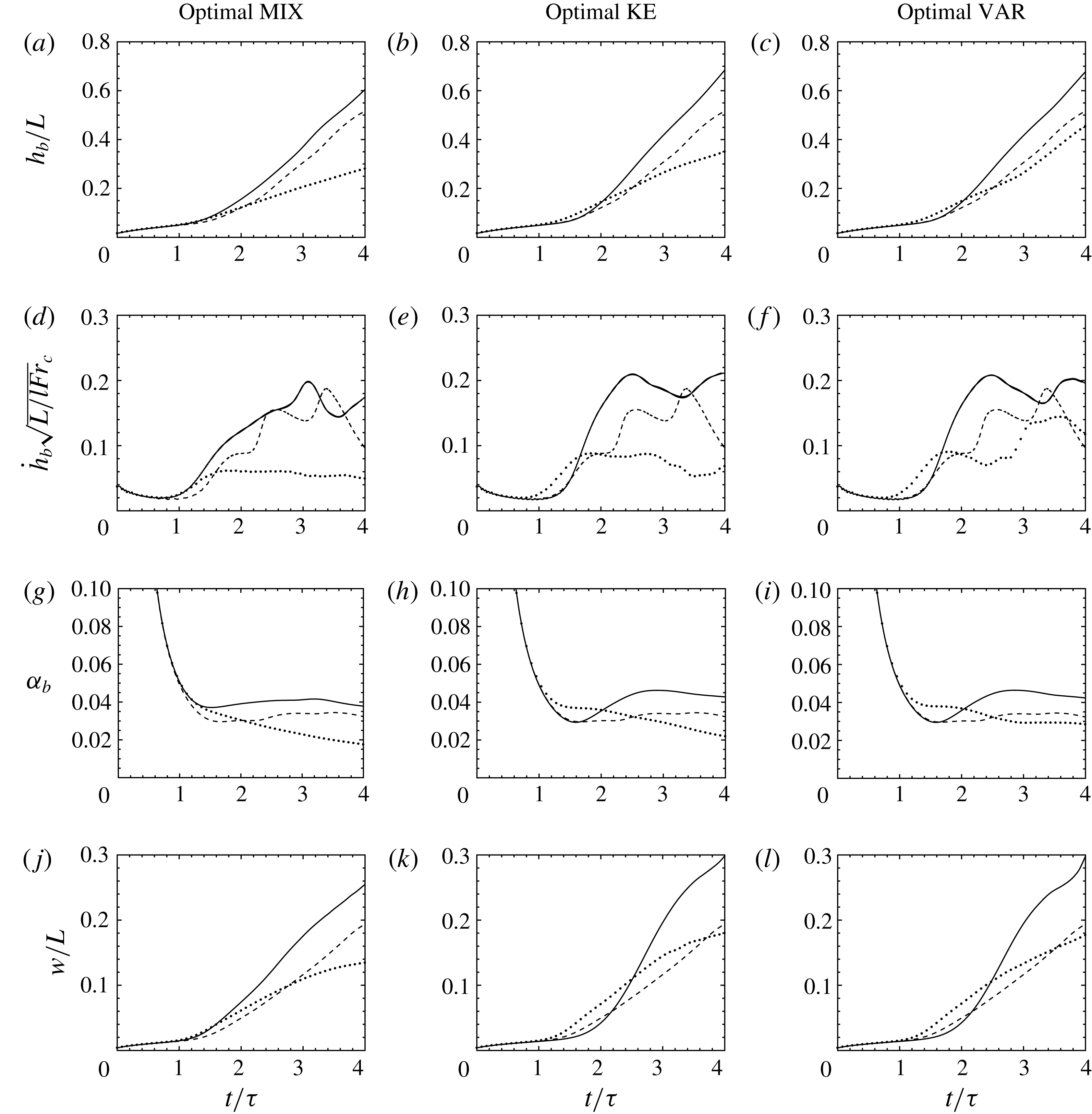
The optimized solutions at $t=4.0\unicode[STIX]{x1D70F}$ for $\text{KE}$ and $\text{VAR}$ exhibit greater fluid penetration compared to the baseline case, while $\text{MIX}$ appears qualitatively to be more mixed (see figure 13). The optimized solutions admit enhancement in conventional measures for RT mixing as well (see figure 14). The values of $\unicode[STIX]{x1D6FC}_{b}$ at $t=4\unicode[STIX]{x1D70F}$ are increased by 17 %, 32 % and 31 %, with respect to the baseline case for $\text{MIX}$ , $\text{KE}$ and $\text{VAR}$ , respectively. The mixing width $w$ was also increased by as much as 54 % compared with the baseline case. It is notable that although $k\approx 8$ corresponds to the most, according to linear stability theory, unstable wavenumber and is thus the fastest growing mode during the EG stage, a single-mode initial perturbation of $k=8$ is not sufficient to optimize growth at later times.

Figure 14.

Evolution of (a–c) bubble height, (d–f) bubble tip velocity, (g–i) bubble growth parameter and (j–l) mixing width of the uniform distribution solution (– –), from the optimized solution over duration $t_{f}=2\unicode[STIX]{x1D70F}~(\cdots \,)$ and $t_{f}=4\unicode[STIX]{x1D70F}$ (–).

The effect of the time duration over which the objective function is computed ( $t_{f}$ ) on enhancing mixing is also studied. The optimization of the three forms of ${\mathcal{J}}$ over duration $t_{f}=2\unicode[STIX]{x1D70F}$ is performed. At this stage of the instability the bubble tip velocity was observed to saturate due to nonlinearities (see figure 10 b). Evolution of RT growth ( $h_{b}$ , ${\dot{h}}_{b}$ and $\unicode[STIX]{x1D6FC}_{b}$ ) and mixing width $w$ corresponding to the optimal values of ${\mathcal{J}}$ over duration $t_{f}=2\unicode[STIX]{x1D70F}$ are compared with the baseline case and the enhanced values over duration $t_{f}=4\unicode[STIX]{x1D70F}$ (see figure 14). While the optimized $t_{f}=2\unicode[STIX]{x1D70F}$ solutions predict larger values for some of the quantities when $t<2\unicode[STIX]{x1D70F}$ , they are found to be suboptimal when $t\gtrsim 2\unicode[STIX]{x1D70F}$ compared to the solutions optimized for $t_{f}=4\unicode[STIX]{x1D70F}$ . Interestingly, the initial perturbations optimized for $t_{f}=2\unicode[STIX]{x1D70F}$ were found to be suboptimal compared to the baseline solution when $t\gtrsim 2\unicode[STIX]{x1D70F}$ as well. For the baseline case, low wavenumber initial perturbations and nonlinear mode-coupling effects augment RT growth at later times, while they are not as present in the optimal $t_{f}=2\unicode[STIX]{x1D70F}$ solutions. These differences become more obvious by observing the evolution of the mole fraction of optimal $\text{VAR}$ for $t_{f}=2\unicode[STIX]{x1D70F}$ and $t_{f}=4\unicode[STIX]{x1D70F}$ (see figure 15). Initially, there is more fluid penetration in the optimal $t_{f}=2\unicode[STIX]{x1D70F}$ solution as the initial perturbation assigns more energy to wavenumbers close to the most unstable mode predicted by linear stability theory. However, at later times, the lower wavenumber modes grow faster. These results indicate that optimization of late-time stages of RT instabilities requires late-time sensitivity information.

Figure 15.

Evolution of mole fraction using the optimized perturbation amplitudes that maximize $\text{VAR}$ over duration (a–d) $t_{f}=2\unicode[STIX]{x1D70F}$ and (e–h) $t_{f}=4\unicode[STIX]{x1D70F}$ . Same colour scheme as figure 2.

5.4 Enhancing three-dimensional mixing using optimal two-dimensional perturbations

Here we evaluate the ability to enhance mixing of a three-dimensional RT instability using the optimal interfacial perturbations determined from the two-dimensional simulations in § 5.3. The initial perturbation energy shown in figure 12(b) is used to initialize the three-dimensional configuration presented in § 4. The optimized amplitudes $A_{m}$ in two dimensions are transformed into $A_{m,n}$ in three dimensions by ensuring the average wavenumber components $k=\sqrt{k_{x}^{2}+k_{z}^{2}}$ are approximately equal to the values obtained from the two-dimensional enhanced solution.

Figure 16.

Evolution of mole fraction using the optimized perturbation amplitudes that maximize $\text{VAR}$ . Same colour scheme as figure 2.

The evolution of the mole fraction using the interfacial perturbations that optimize $\text{VAR}$ is shown in figure 16. It can immediately be seen that substantial mixing and penetration is achieved compared to the baseline solution over the same time horizon (see figure 2). Despite being initialized with the same perturbation energy in two dimensions, compared to the evolution in two dimensions (figure 15 e–h), the flow exhibits three-dimensional behaviour as early as $t=2\unicode[STIX]{x1D70F}$ , resulting in significantly more mixing compared to its two-dimensional counterpart. Figure 17 shows the conventional measures of mixing corresponding to the enhanced objective functions compared to the baseline case. Overall, significant increase in growth and mixing is observed. The objective functions are increased by factors of 1.7, 5.8 and 3.4 for $\text{MIX}$ , $\text{KE}$ and $\text{VAR}$ , respectively, compared to the three-dimensional baseline case reported in § 4. Interestingly, greater enhancement is observed for two of the objective functions compared to the enhanced two-dimensional solutions, which were increased by factors of 1.4, 8.9 and 3.1 for $\text{MIX}$ , $\text{KE}$ and $\text{VAR}$ , respectively. As shown in figures 17(a) and 17(b), the top and bottom walls act to decelerate the bubble heights and bubble tip velocities at later times. Thus, even greater enhancement might be achieved if a larger domain size was considered.

Figure 17.

Evolution of (a) bubble height, (b) bubble tip velocity, (c) bubble growth parameter and (d) mixing width of the three-dimensional RT instabilities with the baseline case (– –) and with the initial interfacial perturbations of the enhanced two-dimensional RT instabilities of $\text{MIX}$ (–○–), $\text{KE}$ (–▫–) and $\text{VAR}$ (–▵–).