1 Introduction
Momentum, heat and mass transfers across gas–liquid interfaces are often seen in many geophysical and industrial processes. For example, it is well known that the heat transfer across the air–sea interface affects the weather, including the development and decay of tropical cyclones (e.g. Emanuel Reference Emanuel1986). Hence, it is important to understand such heat transfer mechanisms and model them for the precise prediction of weather. To clarify the air–sea heat transfer mechanism, and to precisely evaluate the level of heat transfer, researchers have conducted field observations (e.g. Friehe & Schmitt Reference Friehe and Schmitt1976; Large & Pond Reference Large and Pond1982; DeCosmo et al.
Reference DeCosmo, Katsaros, Smith, Anderson, Oost, Bumke and Chadwick1996; Pedreros et al.
Reference Pedreros, Dardier, Dupuis, Graber, Drennan, Weill and Nacass2003; Zhang et al.
Reference Zhang, Black, French and Drennan2008; Richter & Stern Reference Richter and Stern2014) and laboratory experiments using wind–wave tanks (e.g. Garratt & Hyson Reference Garratt and Hyson1975; Hasse et al.
Reference Hasse, Grunewald, Wucknitz, Dunckel and Schriever1978; Ocampo-Torres et al.
Reference Ocampo-Torres, Donelan, Merzi and Jia1994; Drennan et al.
Reference Drennan, Zhang, French, Mccormick and Black2007; Komori et al.
Reference Komori, Kurose, Takagaki, Ohtsubo, Iwano, Handa, Shimada, Komori, McGillis and Kurose2011; Iwano Reference Iwano2014). Based on field observations in oceans and lakes using several instruments (ships, buoys, towers, sonic anemometries, thermistors, hygrometers, etc.), it has been reported that the heat transfer is enhanced by wind shear, and that the latent/sensible heat transfer coefficients have a constant value. On the other hand, Ocampo-Torres et al. (Reference Ocampo-Torres, Donelan, Merzi and Jia1994) have conducted laboratory experiments using the Göttingen-type wind–wave tank, called the Gas Transfer Flume (GTF), of the Hydraulics Laboratory at the National Water Research Institute, having a test section of 32.2 m length and 0.76 m width. They have measured the time change in the water vapour on the gas side, and have estimated the latent heat transfer coefficients. In contrast to the results obtained from field observations (e.g. Friehe & Schmitt Reference Friehe and Schmitt1976; Large & Pond Reference Large and Pond1982; DeCosmo et al.
Reference DeCosmo, Katsaros, Smith, Anderson, Oost, Bumke and Chadwick1996; Pedreros et al.
Reference Pedreros, Dardier, Dupuis, Graber, Drennan, Weill and Nacass2003; Zhang et al.
Reference Zhang, Black, French and Drennan2008), they have shown that the latent heat transfer coefficient increases with increasing wind speed. Further, Zappa, Asher & Jessup (Reference Zappa, Asher and Jessup2004) have measured the heat transfer coefficients in a wind-wave flume, having a test section of 18.29 m length and 0.91 m width, at the Air–Sea Interaction Research Facility at NASA GSFC/WFF. They have developed the active controlled flux technique (ACFT) for measuring the heat transfer coefficients. In the ACFT, the water surface is heated with a high-power (25 W) continuous
 $\text{CO}_{2}$
laser to make a heated spot, and then the time change in surface temperature on the heated spot can be tracked by infrared imagery. They concluded that the heat transfer coefficient correlates with the fractional area coverage of microscale wave breaking, which was computed from infrared imagery. However, because of the difficulty in the measurement of the turbulent flow and temperature field near the gas–liquid interface in field observations and laboratory experiments, the detailed gas–liquid heat transfer mechanism has not been fully clarified yet.
Direct numerical simulation (DNS) is useful for the investigation of such gas–liquid two-phase turbulent flows with wind-driven wavy interfaces. The heat and mass transfer across mobile/immobile gas–liquid interfaces with/without wind shear has been the subject of many numerical investigations (e.g. Komori et al.
Reference Komori, Nagaosa, Murakami, Chiba, Ishii and Kuwahara1993a
; Lakehal et al.
Reference Lakehal, Fulgosi, Yadigaroglu and Banerjee2003; Banerjee, Lakehal & Fulgosi Reference Banerjee, Lakehal and Fulgosi2004; Yamamoto et al.
Reference Yamamoto, Kunugi, Satake and Serizawa2004; Lakehal, Fulgosi & Yadigaroglu Reference Lakehal, Fulgosi and Yadigaroglu2008a
,Reference Lakehal, Fulgosi and Yadigaroglu
b
; Komori et al.
Reference Komori, Kurose, Iwano, Ukai and Suzuki2010; Kermani et al.
Reference Kermani, Khakpour, Shen and Igusa2011; Tsai et al.
Reference Tsai, Chen, Lu and Garbe2013; Guo & Shen Reference Guo and Shen2014; Takagaki et al.
Reference Takagaki, Kurose, Tsujimoto, Komori and Takahashi2015). Using DNS treating a mobile gas–liquid interface with wind shear, Lakehal et al. (Reference Lakehal, Fulgosi, Yadigaroglu and Banerjee2003) have predicted the sensible heat transfer across the sheared gas–liquid interface under the conditions of small-scale interfacial deformation (wave slope
 $ak=0.01$
and
 $k=1{-}3~\text{cm}^{-1}$
, where
 $a$
is wave amplitude and
 $k$
is the wavenumber) by employing an arbitrary Lagrangian–Eulerian (ALE) method. They have found that the sensible heat transfer coefficient, normalized by the friction velocity, decreases with increasing Prandtl number. In addition, using the same numerical techniques, Banerjee et al. (Reference Banerjee, Lakehal and Fulgosi2004) and Lakehal et al. (Reference Lakehal, Fulgosi and Yadigaroglu2008a
,Reference Lakehal, Fulgosi and Yadigaroglu
b
) have investigated the scalar transfer across a sheared gas–liquid interface under a variety of wind and wave conditions. Banerjee et al. (Reference Banerjee, Lakehal and Fulgosi2004) have simulated the large-scale interfacial deformation (
 $ak=0.12$
and
 $k=1{-}3~\text{cm}^{-1}$
), and have investigated the relationship between the surface divergence and the mass transfer coefficient on the liquid side. They have proposed a surface-divergence model for the mass transfer across the sheared gas–liquid interface. On the other hand, Lakehal et al. (Reference Lakehal, Fulgosi and Yadigaroglu2008a
,Reference Lakehal, Fulgosi and Yadigaroglu
b
) have simulated the small-scale interfacial deformation (
 $ak=0.01$
and
 $k=1{-}3~\text{cm}^{-1}$
; which is the same as in the study by Lakehal et al.
Reference Lakehal, Fulgosi, Yadigaroglu and Banerjee2003) with latent/sensible heat transfer across the gas–liquid interface. They have proposed two new scaling laws for the normalized heat transfer coefficient on both the gas and liquid sides. Further, Yamamoto et al. (Reference Yamamoto, Kunugi, Satake and Serizawa2004) have predicted the gas–liquid interface deformation and sensible heat transfer across a sheared gas–liquid interface by DNS with the multi-interface advection and reconstruction solver (MARS) (Kunugi Reference Kunugi1997), which is a variant of the volume of fluids method. Komori et al. (Reference Komori, Kurose, Iwano, Ukai and Suzuki2010) and Takagaki et al. (Reference Takagaki, Kurose, Tsujimoto, Komori and Takahashi2015) have predicted the mass transfer across a sheared gas–liquid interface using DNS with the ALE method, and have investigated the effects of turbulent eddies and Langmuir circulations on the mass transfer across the wavy gas–liquid interface. Here, the Langmuir circulations are longitudinal vortices aligned with the wind on the liquid side and provide surface convergence flows, which are visualized by oils, leaves and bubbles in nature. Langmuir circulations can be induced by the interaction of Stokes drift and shear; that is, the driving force of the surface convergence flows is induced by Stokes drift and shear (Craik & Leibovich Reference Craik and Leibovich1976; Leibovich Reference Leibovich1983; Thorpe Reference Thorpe2004). Tsai et al. (Reference Tsai, Chen, Lu and Garbe2013) have performed DNS of the turbulent liquid flow beneath non-breaking gravity–capillary waves, in which simplified driving shear stress and surface-normal pressure on the liquid side are given without coupling the gas and liquid flows. They have concluded that the scalar transfer across the gas–liquid interface is controlled by both the turbulent eddies and Langmuir circulations. Thus, although many studies have investigated fluid motions and scalar transfer across sheared gas–liquid interfaces, there are few studies on the detailed mechanism of heat transfer across sheared gas–liquid interfaces. In fact, Lakehal et al. (Reference Lakehal, Fulgosi, Yadigaroglu and Banerjee2003), Banerjee et al. (Reference Banerjee, Lakehal and Fulgosi2004), Yamamoto et al. (Reference Yamamoto, Kunugi, Satake and Serizawa2004) and Tsai et al. (Reference Tsai, Chen, Lu and Garbe2013) have ignored the latent heat transfer across the gas–liquid interface due to evaporation. Moreover, Lakehal et al. (Reference Lakehal, Fulgosi and Yadigaroglu2008a
,Reference Lakehal, Fulgosi and Yadigaroglu
b
) have investigated the latent/sensible heat transfer across a sheared gas–liquid interface, but the interfacial deformation considered was small (
 $ak=0.01$
and
 $k=1{-}3~\text{cm}^{-1}$
) and the effect of Langmuir circulation was not considered.
The purpose of this study is, therefore, to investigate the latent/sensible heat transfer across a sheared wind-driven gas–liquid interface by DNS of gas–liquid two-phase turbulent flows with a wind-driven non-breaking wavy interface with a large-scale interfacial deformation (
 $ak=0.2$
and
 $k=1.4~\text{cm}^{-1}$
). To precisely evaluate the relationship between turbulent structures with Langmuir circulations and gas–liquid heat transfer in realistic wind-driven turbulence, the development of wind waves from a stationary state is simulated by coupling the gas and liquid flows, as in the studies by Komori et al. (Reference Komori, Kurose, Iwano, Ukai and Suzuki2010) and Takagaki et al. (Reference Takagaki, Kurose, Tsujimoto, Komori and Takahashi2015).
2 Numerical simulation
The wind-driven wavy gas–liquid interface was captured using a free-surface reconstruction method, namely the ALE method with boundary-fitted coordinates (BFCs) on moving grids (Komori et al. Reference Komori, Nagaosa, Murakami, Chiba, Ishii and Kuwahara1993a , Reference Komori, Kurose, Iwano, Ukai and Suzuki2010; Fulgosi et al. Reference Fulgosi, Lakehal, Banerjee and De Angelis2003; Lakehal et al. Reference Lakehal, Fulgosi, Yadigaroglu and Banerjee2003, Reference Lakehal, Fulgosi and Yadigaroglu2008a ,Reference Lakehal, Fulgosi and Yadigaroglu b ; Banerjee et al. Reference Banerjee, Lakehal and Fulgosi2004; Lin et al. Reference Lin, Moeng, Tsai, Sullivan and Belcher2008; Tsai et al. Reference Tsai, Chen, Lu and Garbe2013; Guo & Shen Reference Guo and Shen2014; Takagaki et al. Reference Takagaki, Kurose, Tsujimoto, Komori and Takahashi2015). The numerical procedure of the DNS used here was the same as in the study by Komori et al. (Reference Komori, Kurose, Iwano, Ukai and Suzuki2010).
The non-dimensional governing equations for an incompressible Newtonian fluid flow with heat transfer are given by the equation of continuity, the Navier–Stokes (N–S) equation and the transport equations of heat and moisture as passive scalars using the Einstein summation convention:
 $$\begin{eqnarray}\displaystyle & \displaystyle \frac{\unicode[STIX]{x2202}U_{i}}{\unicode[STIX]{x2202}x_{i}}=0, & \displaystyle\end{eqnarray}$$
 $$\begin{eqnarray}\displaystyle & \displaystyle \frac{\unicode[STIX]{x2202}U_{i}}{\unicode[STIX]{x2202}t}+U_{j}\frac{\unicode[STIX]{x2202}U_{i}}{\unicode[STIX]{x2202}x_{j}}=-\frac{\unicode[STIX]{x2202}p}{\unicode[STIX]{x2202}x_{i}}+\frac{1}{Re}\frac{\unicode[STIX]{x2202}^{2}U_{i}}{\unicode[STIX]{x2202}x_{j}\unicode[STIX]{x2202}x_{j}}+\frac{1}{Fr}\unicode[STIX]{x1D6FF}_{i3}, & \displaystyle\end{eqnarray}$$
 $$\begin{eqnarray}\displaystyle & \displaystyle \frac{\unicode[STIX]{x2202}T}{\unicode[STIX]{x2202}t}+U_{j}\frac{\unicode[STIX]{x2202}T}{\unicode[STIX]{x2202}x_{j}}=\frac{1}{Re\cdot Pr}\frac{\unicode[STIX]{x2202}^{2}T}{\unicode[STIX]{x2202}x_{j}\unicode[STIX]{x2202}x_{j}}, & \displaystyle\end{eqnarray}$$
 $$\begin{eqnarray}\displaystyle & \displaystyle \frac{\unicode[STIX]{x2202}q}{\unicode[STIX]{x2202}t}+U_{j}\frac{\unicode[STIX]{x2202}q}{\unicode[STIX]{x2202}x_{j}}=\frac{1}{Re\cdot Sc}\frac{\unicode[STIX]{x2202}^{2}q}{\unicode[STIX]{x2202}x_{j}\unicode[STIX]{x2202}x_{j}}, & \displaystyle\end{eqnarray}$$
 $U_{i}$
is the
 $i$
th component of the velocity vector (
 $i=1$
, 2, and 3 denote the streamwise, spanwise and vertical directions respectively),
 $p$
is the pressure,
 $\unicode[STIX]{x1D6FF}_{ij}$
is the Kronecker delta,
 $T$
is the temperature, and
 $q$
is the specific humidity. Here, (2.4) is solved only on the gas side. The non-dimensional parameters, namely the Reynolds number
 $Re$
, Prandtl number
 $Pr$
, Schmidt number
 $Sc$
and Froude number
 $Fr$
, are defined as
 $$\begin{eqnarray}\displaystyle Re=\frac{U_{0}L_{0}}{\unicode[STIX]{x1D708}},\quad Pr=\frac{\unicode[STIX]{x1D708}}{\unicode[STIX]{x1D6FC}},\quad Sc=\frac{\unicode[STIX]{x1D708}}{D},\quad Fr=\frac{U_{0}^{2}}{gL_{0}}, & & \displaystyle\end{eqnarray}$$
where
 $L_{0}$
and
 $U_{0}$
are the reference length and velocity respectively,
 $\unicode[STIX]{x1D708}$
is the kinematic viscosity,
 $\unicode[STIX]{x1D6FC}$
is the thermal diffusivity,
 $D$
is the molecular diffusivity of moisture on the gas side and
 $g$
is the acceleration due to gravity.
Boundary conditions at the gas–liquid interface.

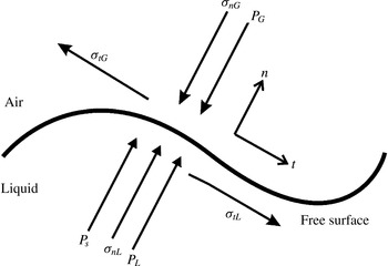
On the gas–liquid interface, two boundary conditions should be satisfied, as shown in figure 1. One is the kinematic boundary condition that describes the Lagrangian behaviour of the fluid particle on the mobile gas–liquid interface:
 $$\begin{eqnarray}\displaystyle \frac{\unicode[STIX]{x2202}f}{\unicode[STIX]{x2202}t}+U_{1}\frac{\unicode[STIX]{x2202}f}{\unicode[STIX]{x2202}x_{1}}+U_{2}\frac{\unicode[STIX]{x2202}f}{\unicode[STIX]{x2202}x_{2}}=U_{3}, & & \displaystyle\end{eqnarray}$$
where
 $f$
is the function representing the deformation of the interface. The other is the dynamic boundary condition, which is determined from the balance of stresses acting on the gas–liquid interface in the normal and tangential directions:
 $$\begin{eqnarray}\displaystyle & \displaystyle \left.\begin{array}{@{}c@{}}\displaystyle p_{L}+\unicode[STIX]{x1D70E}_{nL}+p_{s}=p_{G}+\unicode[STIX]{x1D70E}_{nG},\\ \displaystyle \unicode[STIX]{x1D70E}_{n}=\frac{1}{Re}e_{ij}n_{j}n_{i},\\ \displaystyle p_{s}=\unicode[STIX]{x1D6FE}k_{m},\end{array}\right\} & \displaystyle\end{eqnarray}$$
 $$\begin{eqnarray}\displaystyle & \displaystyle \left.\begin{array}{@{}c@{}}\displaystyle \unicode[STIX]{x1D70E}_{tL}=\unicode[STIX]{x1D70E}_{tG},\\ \displaystyle \unicode[STIX]{x1D70E}_{t}=\frac{1}{Re}e_{ij}n_{j}t_{i},\end{array}\right\} & \displaystyle\end{eqnarray}$$
 $\unicode[STIX]{x1D70E}_{n}$
,
 $\unicode[STIX]{x1D70E}_{t}$
,
 $p_{s}$
,
 $e_{ij}$
,
 $\unicode[STIX]{x1D6FE}$
,
 $k_{m}$
,
 $n_{i}$
and
 $t_{i}$
are the normal component of the viscous force vector, the tangential component of the viscous force vector, the pressure variation caused by the surface tension, the deformation rate tensor, the surface tension coefficient, the mean curvature of the free surface, the wall-normal unit vector and the wall-tangential unit vector respectively. Subscripts
 $G$
and
 $L$
indicate the gas and liquid sides respectively.
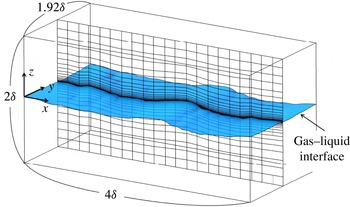
The computational domain and grids depicted coarsely. Here,
 $\unicode[STIX]{x1D6FF}$
is the height of the computational domain on the gas side, and
 $\unicode[STIX]{x1D6FF}$
equals
 $2.5\times 10^{-2}$
m.

The computational domain and numerical grids for the computation of flows on the gas and liquid sides are shown in figure 2. The size of the computational domain was
 $4.0\unicode[STIX]{x1D6FF}\times 1.92\unicode[STIX]{x1D6FF}\times 2.0\unicode[STIX]{x1D6FF}$
in the streamwise (
 $x$
), spanwise (
 $y$
) and vertical (
 $z$
) directions. The origin (
 $x=y=z=0$
) was located at a height of
 $1\unicode[STIX]{x1D6FF}$
from the bottom, and the initial flat gas–liquid interface, which divides the two-phase flow between the upper gas and lower liquid streams, was placed on the plane
 $z=0$
. The grid points used in the streamwise (
 $x$
), spanwise (
 $y$
) and vertical (
 $z$
) directions were
 $200\times 96\times 120$
on the gas side and
 $200\times 96\times 120$
on the liquid side. The grid spacing was equidistant in the streamwise (
 $x$
) and spanwise (
 $y$
) directions, and to get high resolution, non-uniform meshes, clustered in the gas–liquid-interface region, were used in the vertical (
 $z$
) direction. Periodic boundary conditions were applied in the streamwise (
 $x$
) and spanwise (
 $y$
) directions, and slip boundary conditions were applied at the top and bottom boundaries. The mesh sizes were chosen according to the results of previous studies (Komori et al.
Reference Komori, Kurose, Iwano, Ukai and Suzuki2010; Takagaki et al.
Reference Takagaki, Kurose, Tsujimoto, Komori and Takahashi2015) and also according to the mesh size in the wall turbulent flow (e.g.
 $\unicode[STIX]{x0394}z^{+}<1$
near the surface;
 $\unicode[STIX]{x0394}x$
,
 $\unicode[STIX]{x0394}y$
,
 $\unicode[STIX]{x0394}z\sim \unicode[STIX]{x1D702}$
, where
 $\unicode[STIX]{x1D702}$
is the Kolmogorov scale). However,
 $\unicode[STIX]{x1D702}$
near the interface on the gas and liquid sides could not be evaluated using the predicted data, because precise prediction of the length scales near a mobile gas–liquid interface is difficult. We could, nevertheless, approximate them based on experimental data (Takagaki Reference Takagaki2009) as
 $\unicode[STIX]{x1D702}_{G}=10^{-5}$
m and
 $\unicode[STIX]{x1D702}_{L}=10^{-4}$
m on the gas and liquid sides respectively. Additionally, the Batchelor scale,
 $B_{L}$
, on the liquid side was 0.47 higher than
 $\unicode[STIX]{x1D702}_{L}$
on the liquid side, according to the relation
 $B_{L}=\unicode[STIX]{x1D702}_{L}Pr_{L}^{-0.5}$
(here, the Prandtl number,
 $Pr_{L}$
, is 4.6 on the liquid side). Accordingly,
 $B_{L}$
was estimated to be
 $4.7\times 10^{-5}$
m. In the present simulation, the vertical grid scale near the gas–liquid interface on the liquid side was
 $2.4\times 10^{-5}$
m. This means that the grid scale near the gas–liquid interface on the liquid side was adequate to visualize the scalar fluctuations by using the Batchelor scale. Moreover, the spatial scale of free-surface perturbations, that is the wavelength, was 0.0460 m, as explained in table 1. Thus, the scale of free-surface perturbations was 460 and 46 times larger than the Kolmogorov scale near the interface on the gas and liquid sides respectively.
Predicted characteristics of the gas flow and wind waves. Here,
 $t$
is the elapsed time,
 $U_{\infty }$
is the free-stream wind speed,
 $u_{G}^{\ast }$
is the friction velocity on the gas side,
 $U_{10N}$
is the wind speed at 10 m height,
 $C_{DN}$
is the drag coefficient,
 $z_{0}$
is the roughness length,
 $U_{SURF}$
is the surface current,
 $H_{S}$
is the significant wave height,
 $L_{S}$
is the significant wavelength and
 $C_{P}$
is the phase speed of significant wind waves.

For the initial conditions of the flow field, a fully developed wall turbulent flow and a quiescent flow were imposed on both the gas and liquid sides of the flat interface respectively. In the present simulation, a constant pressure gradient (
 $213~\text{N}~\text{m}^{-3}$
) was imposed in the streamwise direction on the gas side as the driving force for maintaining the fully developed boundary layer flow over the gas–liquid interface. The marker and cell method (Harlow & Welch Reference Harlow and Welch1965) was used to solve the Navier–Stokes equation. For discretization, we used a fifth-order upwind difference scheme for the convection terms of the N–S equation (2.2) and the transport (2.3), (2.4) for the heat and moisture. Similarly, a fourth-order central difference scheme was used for discretizing the viscous term of the N–S equation (2.2) and the diffusion term of the transport (2.3), (2.4) for the heat and moisture. A second-order central difference scheme was used for discretizing other terms in the present simulation. The implicit Euler method was used for time integration.
For the computation of heat transfer on both the gas and liquid sides, the initial conditions for temperature were given by 300 K and 310 K, and that for moisture was given by
 $0.015~\text{g}~\text{g}^{-1}$
. In addition, the top boundary conditions for temperature (
 $T_{G}=300~\text{K}$
at the top wall) and moisture (
 $q=0.015~\text{g}~\text{g}^{-1}$
at the top wall) and the bottom boundary condition for temperature (
 $T_{L}=310$
K at the bottom wall) were calculated using the Dirichlet condition. For heat transfer on the gas–liquid interface, calculated using the ALE method with BFCs on moving grids (Komori et al.
Reference Komori, Nagaosa, Murakami, Chiba, Ishii and Kuwahara1993a
, Reference Komori, Kurose, Iwano, Ukai and Suzuki2010; Fulgosi et al.
Reference Fulgosi, Lakehal, Banerjee and De Angelis2003; Lakehal et al.
Reference Lakehal, Fulgosi, Yadigaroglu and Banerjee2003, Reference Lakehal, Fulgosi and Yadigaroglu2008a
,Reference Lakehal, Fulgosi and Yadigaroglu
b
; Banerjee et al.
Reference Banerjee, Lakehal and Fulgosi2004; Lin et al.
Reference Lin, Moeng, Tsai, Sullivan and Belcher2008; Guo & Shen Reference Guo and Shen2014; Tsai et al.
Reference Tsai, Chen, Lu and Garbe2013; Takagaki et al.
Reference Takagaki, Kurose, Tsujimoto, Komori and Takahashi2015), the energy-budget relationship among the total heat flux,
 $Q_{T}$
, latent heat flux,
 $Q_{E}$
, gaseous sensible heat flux,
 $Q_{H}$
(which includes both conduction and convection), and radiative heat flux,
 $Q_{R}$
, is given by
 $$\begin{eqnarray}\displaystyle Q_{T}=Q_{H}+Q_{E}+Q_{R}. & & \displaystyle\end{eqnarray}$$
The four heat fluxes are calculated as
 $$\begin{eqnarray}\displaystyle & \displaystyle Q_{T}=-\unicode[STIX]{x1D6FC}_{L}\unicode[STIX]{x1D70C}_{L}C_{pL}\left.\frac{\unicode[STIX]{x2202}T}{\unicode[STIX]{x2202}n}\right|_{z=0,Liquid\text{-}side}, & \displaystyle\end{eqnarray}$$
 $$\begin{eqnarray}\displaystyle & \displaystyle Q_{H}=-\unicode[STIX]{x1D6FC}_{G}\unicode[STIX]{x1D70C}_{G}C_{pG}\left.\frac{\unicode[STIX]{x2202}T}{\unicode[STIX]{x2202}n}\right|_{z=0,Gas\text{-}side}, & \displaystyle\end{eqnarray}$$
 $$\begin{eqnarray}\displaystyle & \displaystyle Q_{E}=-D\unicode[STIX]{x1D70C}_{G}L_{V}\left.\frac{\unicode[STIX]{x2202}q}{\unicode[STIX]{x2202}n}\right|_{z=0}, & \displaystyle\end{eqnarray}$$
 $$\begin{eqnarray}\displaystyle & \displaystyle Q_{R}=\unicode[STIX]{x1D700}\unicode[STIX]{x1D70E}(T_{i}^{4}-T_{bG}^{4}), & \displaystyle\end{eqnarray}$$
 $\unicode[STIX]{x1D6FC}$
is the thermal diffusivity,
 $\unicode[STIX]{x1D70C}$
is the density,
 $C_{p}$
is the specific heat at constant pressure,
 $\boldsymbol{n}$
is the normal unit vector on the gas–liquid interface,
 $L_{V}$
is the latent heat of vaporization,
 $D$
is the molecular diffusivity of moisture on the gas side,
 $\unicode[STIX]{x1D700}$
is the emissivity against the gas–liquid interface,
 $\unicode[STIX]{x1D70E}$
is the Stefan–Boltzmann constant (
 $=5.67\times 10^{-8}~\text{W}~\text{m}^{-2}~\text{K}^{-4}$
),
 $T_{i}$
is the surface temperature and
 $T_{b}$
is the bulk temperature. The subscripts
 $G$
and
 $L$
represent the gas (humid air) and liquid sides respectively. To compare the results with those of previous studies (Komori et al.
Reference Komori, Kurose, Takagaki, Ohtsubo, Iwano, Handa, Shimada, Komori, McGillis and Kurose2011; Iwano Reference Iwano2014), only long-wave radiative heat flux is considered as the present predicted total radiative heat flux in (2.13). In addition, the temperature gradients on the gas and liquid sides are calculated using (2.10) and (2.11) respectively. The specific-humidity gradient in (2.12) is calculated on the gas side. For calculating the gradients of temperature and specific humidity in (2.10)–(2.12), the following relations among the surface temperature,
 $T_{i}$
, saturation vapour pressure,
 $p_{sat}$
(Tetens Reference Tetens1930), and saturation specific humidity,
 $q_{sat}$
,
 $$\begin{eqnarray}\displaystyle & \displaystyle p_{sat}=6.1078\times 10^{7.5T_{i}/(T_{i}+237.3)}, & \displaystyle\end{eqnarray}$$
 $$\begin{eqnarray}\displaystyle & \displaystyle q_{sat}=\frac{0.622p_{sat}}{p_{atm}-0.378p_{sat}}, & \displaystyle\end{eqnarray}$$
 $q_{i}$
, is defined as
 $q_{i}=q_{sat}$
. We did not consider the decrease in water volume caused by evaporation.
To induce a realistic deformation at the gas–liquid interface, a fully developed wall turbulence with an initial free-stream velocity of
 $U_{\infty ,ini}=5.3~\text{m}~\text{s}^{-1}$
and an initial friction velocity of
 $u_{G,ini}^{\ast }=0.24~\text{m}~\text{s}^{-1}$
was given on the gas side over a flat quiescent liquid. The gas flow was driven by a pressure gradient imposed in the streamwise direction. The value of the Reynolds number based on
 $U_{\infty ,ini}$
and the height of the computational domain on the gas side (
 $\unicode[STIX]{x1D6FF}=2.5\times 10^{-2}$
m),
 $Re_{ini}$
, was 8390, and
 $Re_{ini}^{\ast }$
based on
 $u_{G,ini}^{\ast }$
and
 $\unicode[STIX]{x1D6FF}$
was 380. In addition, the values of the Weber number and Froude number were 9948 and 116 respectively, based on
 $U_{\infty ,ini}$
and the height of the computational domain on the gas side (
 $\unicode[STIX]{x1D6FF}=2.5\times 10^{-2}$
m). The dimensions of the computational domain, normalized by the friction velocity,
 $u_{G,ini}^{\ast }$
, and viscosity,
 $\unicode[STIX]{x1D708}_{G}$
, i.e. wall units, on the gas side, were
 $1643\times 789\times 822$
, and those normalized by the friction velocity,
 $u_{L,ini}^{\ast }$
, and viscosity,
 $\unicode[STIX]{x1D708}_{L}$
, on the liquid side, were
 $1285\times 617\times 642$
in the streamwise (
 $x$
), spanwise (
 $y$
) and vertical (
 $z$
) directions at
 $t=6.0$
s respectively. The liquid/gas density ratio was 844, and the Prandtl number on the gas side,
 $Pr_{G}$
, Prandtl number on the liquid side,
 $Pr_{L}$
, and Schmidt number on the gas side,
 $Sc$
, were 0.7, 4.6 and 0.6 respectively. The physical values of the density,
 $Pr_{G}$
, and
 $Sc$
correspond to the values for the bulk air at 300 K and for the bulk water at 310 K respectively. As detailed in § 3.1, the buoyancy effect is negligibly small in the present flow field on the gas side over the waves. The CPU time was approximately 5400 h (14 days of wall-clock time using 16 cores) for 2 500 000 steps (6.25 s) on the supercomputer NEC : SX-9. We could not conduct the simulation with a larger computational domain and longer CPU time than the present computational setting, because of the limited computational source. However, 6.25 s is considered to be adequate to investigate heat transport across the wavy gas–liquid interface, because the wind-wave turbulent field reaches fully developed turbulent flow at
 $t=6.0$
s, as detailed in §§ 3.1 and 3.2.
3 Results and discussion
3.1 General features of wind-driven turbulence
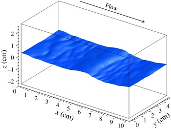
Figure 3 shows the instantaneous configuration of the gas–liquid interface at
 $t=6.0$
s. Wind waves are seen to develop and generate microbreaking waves (i.e. ripples) on the leeward side of the wind waves. A similar wave shape was observed in our previous experiments and predictions, and the details are described in the study by Komori et al. (Reference Komori, Kurose, Iwano, Ukai and Suzuki2010).
Instantaneous configuration of the gas–liquid interface at
 $t=6.0$
s.

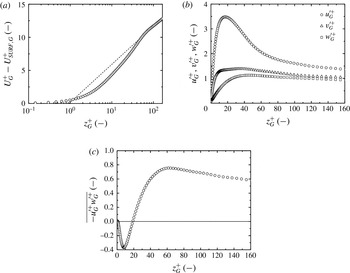
Vertical distributions of (a) normalized mean streamwise velocity,
 $U_{G}^{+}-U_{SURF,G}^{+}$
, (b) normalized streamwise, vertical and spanwise velocity fluctuations,
 $u_{G}^{\prime +}$
,
 $v_{G}^{\prime +}$
and
 $w_{G}^{\prime +}$
, and (c) Reynolds stress,
 $-\overline{u_{G}^{\prime +}w_{G}^{\prime +}}$
, on the gas side at
 $t=6.0$
s. The dashed line in figure 4(a) shows the log law calculated using (3.4). These values are obtained by taking the time average of
 $t=5.75$
–6.25 s and space average in the streamwise and spanwise directions.

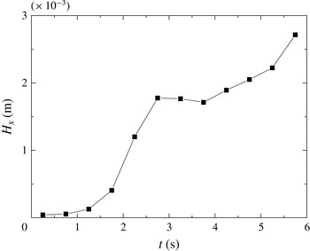
Time change of significant wave height. Here, these values are obtained by taking the time average with 0.5 s and space average in the spanwise direction.

Figure 4 shows the vertical distributions of the mean streamwise velocity,
 $U_{G}^{+}-U_{SURF,G}^{+}$
, streamwise, vertical and spanwise velocity fluctuations,
 $u_{G}^{\prime +}$
,
 $v_{G}^{\prime +}$
and
 $w_{G}^{\prime +}$
respectively, and Reynolds stress,
 $-\overline{u_{G}^{\prime +}w_{G}^{\prime +}}$
, on the gas side, where
 $U_{SURF}$
is the surface current and
 $z=0$
is set to be the location of the instantaneous free surface. The values with superscript ‘
 $+$
’ refer to values in wall units, and those with subscripts
 $G$
and
 $L$
refer to values normalized by the gas and liquid properties respectively. Here, these values are obtained by taking the time average of
 $t=5.75$
–6.25 s and space average in the streamwise and spanwise directions, and are normalized by the friction velocity and viscosity on the gas side,
 $u_{G}^{\ast }$
and
 $\unicode[STIX]{x1D708}_{G}$
. In the figure,
 $z_{G}^{+}$
is the distance from the instantaneous wavy mobile gas–liquid interface, normalized by
 $u_{G}^{\ast }$
and
 $\unicode[STIX]{x1D708}_{G}$
. Here,
 $u_{G}^{\ast }$
is estimated in the same manner as done by Komori et al. (Reference Komori, Kurose, Iwano, Ukai and Suzuki2010), i.e. by the total drag on the gas side. The total drag,
 $\unicode[STIX]{x1D70F}_{T}$
, is defined as
 $$\begin{eqnarray}\displaystyle \unicode[STIX]{x1D70F}_{T}=\unicode[STIX]{x1D70F}_{F}+\unicode[STIX]{x1D70F}_{P}, & & \displaystyle\end{eqnarray}$$
where the friction drag,
 $\unicode[STIX]{x1D70F}_{F}$
, and pressure drag,
 $\unicode[STIX]{x1D70F}_{P}$
, are defined as
 $$\begin{eqnarray}\displaystyle & \displaystyle \unicode[STIX]{x1D70F}_{F}=\frac{1}{A}\iint _{S}\tilde{\unicode[STIX]{x1D70E}}_{t}\boldsymbol{t}\boldsymbol{\cdot }\boldsymbol{e}_{\boldsymbol{x}}\,\text{d}S, & \displaystyle\end{eqnarray}$$
 $$\begin{eqnarray}\displaystyle & \displaystyle \unicode[STIX]{x1D70F}_{P}=\frac{1}{A}\iint _{S}(\tilde{p}+\tilde{\unicode[STIX]{x1D70E}}_{n})\boldsymbol{n}\boldsymbol{\cdot }\boldsymbol{e}_{\boldsymbol{x}}\,\text{d}S. & \displaystyle\end{eqnarray}$$
 $\boldsymbol{n}$
,
 $\boldsymbol{t}$
and
 $\boldsymbol{e}_{\boldsymbol{x}}$
are the wall normal unit vector, the wall tangential unit vector and the streamwise unit vector respectively. Hereafter, the other turbulent statistics in the following figures and tables will be calculated in the same way. In figure 4, it is found that these profiles are similar to those in the wall turbulent boundary layers, except for the existence of the peak of
 $-\overline{u_{G}^{\prime +}w_{G}^{\prime +}}$
near the interface. The negative peak originates from the wake on the leeward side of the wind waves (Komori et al.
Reference Komori, Kurose, Iwano, Ukai and Suzuki2010). The conditions of the gas flow and wind waves are listed in table 1. Here, the uniform velocity on the gas side,
 $U_{\infty }$
, is defined as the velocity on the upper wall of the computational domain. The roughness length,
 $z_{0}$
, is estimated using the logarithmic profile (e.g. Jones & Toba Reference Jones and Toba2001) at a neutral stratification along with the wind speed at
 $z$
as
 $$\begin{eqnarray}\displaystyle U(z)-U_{SURF}=\frac{u_{G}^{\ast }}{\unicode[STIX]{x1D705}}\ln \frac{z}{z_{0}}, & & \displaystyle\end{eqnarray}$$
where
 $\unicode[STIX]{x1D705}$
is the von Karman constant. Similarly, the wind speed at 10 m height above the gas–liquid interface,
 $U_{10N}$
, is estimated by
 $$\begin{eqnarray}\displaystyle U_{10N}-U_{SURF}=\frac{u_{G}^{\ast }}{\unicode[STIX]{x1D705}}\ln \frac{10}{z_{0}}. & & \displaystyle\end{eqnarray}$$
Then, the drag coefficient,
 $C_{DN}$
, is estimated from the definition shown as
 $$\begin{eqnarray}\displaystyle \unicode[STIX]{x1D70F}_{T}=\unicode[STIX]{x1D70C}_{G}u_{G}^{\ast 2}=\unicode[STIX]{x1D70C}_{a}C_{DN}U_{10N}^{2}, & & \displaystyle\end{eqnarray}$$
where the total drag,
 $\unicode[STIX]{x1D70F}_{T}$
, is calculated from (3.1)–(3.3). Each wind wave is determined by applying the zero-up cross method to the spatial fluctuation of the water level. The significant wave height,
 $H_{S}$
, and significant wavelength,
 $L_{S}$
, are defined as the mean wave height and length respectively for the largest one-third waves. The phase speed of the significant wind waves,
 $C_{p}$
, is measured by analysing the propagation of the significant wind waves. Here, these values are obtained by taking the time average with 0.5 s and space average in the spanwise direction. Figure 5 shows the time change of the significant wave height,
 $H_{S}$
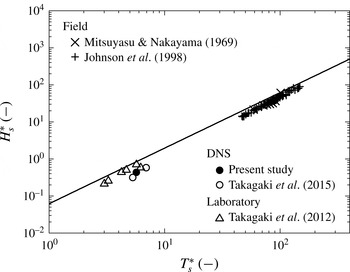
. Figure 6 shows the relationship between the non-dimensional significant wave height,
 $H_{S}^{\ast }=H_{S}g/u_{G}^{\ast 2}$
, and the non-dimensional significant wave period,
 $T_{S}^{\ast }=T_{S}g/u_{G}^{\ast }$
, together with Toba’s
 $3/2$
law (Toba Reference Toba1972), which is confirmed to be consistent with both laboratory data (e.g. Takagaki et al.
Reference Takagaki, Komori, Suzuki, Iwano, Kuramoto, Shimada, Kurose and Takahashi2012) and field data (e.g. Mitsuyasu & Nakayama Reference Mitsuyasu and Nakayama1969; Johnson et al.
Reference Johnson, Hojstrup, Vested and Larsen1998). Here, the significant wave period,
 $T_{S}$
, is estimated by
 $T_{S}=L_{S}/C_{P}$
, and these values are obtained by taking the time average of
 $t=5.75$
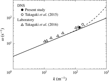
–6.25 s. Further, figure 7 shows the relationship between the significant wave angular frequency,
 $\unicode[STIX]{x1D714}=2\unicode[STIX]{x03C0}/T_{S}$
, and significant wavenumber,
 $k=2\unicode[STIX]{x03C0}/L_{S}$
. Although the predicted significant wind waves gradually increase with time (see figure 5) and are Doppler-shifted by the surface current (see figure 7), the statistical properties of the wind waves are confirmed to be consistent with our laboratory data (Takagaki et al.
Reference Takagaki, Komori, Suzuki, Iwano, Kuramoto, Shimada, Kurose and Takahashi2012; Takagaki, Komori & Suzuki Reference Takagaki, Komori and Suzuki2016), Toba’s
 $3/2$
law and the dispersed relation for capillary–gravity waves (Lamb Reference Lamb1932). This means that the predicted surface waves reach general wind waves as defined by Toba’s
 $3/2$
law and the dispersed relation at
 $t=6.0$
s. Moreover, turbulent fluctuations are hardly affected by such time change of wind waves (figure 5), as explained in figure 31.
Non-dimensional significant wave height,
 $H_{S}^{\ast }$
, versus non-dimensional significant wave period,
 $T_{S}^{\ast }$
. The line shows Toba’s
 $3/2$
power law (Toba Reference Toba1972). Here, these values are obtained by taking the time average of
 $t=5.75$
–6.25 s and space average in the spanwise direction.

Dispersion relations: the solid and dotted lines show the dispersion relations for gravity waves and capillary–gravity waves (Lamb Reference Lamb1932) respectively. Here, these values are obtained by taking the time average of
 $t=5.75$
–6.25 s and space average in the spanwise direction.

In the present non-isothermal conditions, the flow field on the gas side is only slightly affected by buoyancy. In the following, the effect of buoyancy is discussed. In this case, instead of (3.4), the wind profiles can be estimated by
 $$\begin{eqnarray}\displaystyle U(z)-U_{SURF}=\frac{u_{G}^{\ast }}{\unicode[STIX]{x1D705}}\left(\ln \frac{z}{z_{0}}-\unicode[STIX]{x1D6F9}_{u}(\unicode[STIX]{x1D709})\right), & & \displaystyle\end{eqnarray}$$
where
 $\unicode[STIX]{x1D6F9}_{u}(\unicode[STIX]{x1D709})$
is the profile parameter for momentum transfer;
 $\unicode[STIX]{x1D709}$
is defined as
 $\unicode[STIX]{x1D709}=z/L$
using the Monin–Obukhov length,
 $L$
,
 $$\begin{eqnarray}\displaystyle L=\frac{-u_{G}^{\ast 3}\unicode[STIX]{x1D6E9}_{v}}{\unicode[STIX]{x1D705}g\overline{w^{\prime }\unicode[STIX]{x1D703}_{v}^{\prime }}}, & & \displaystyle\end{eqnarray}$$
where
 $\unicode[STIX]{x1D6E9}_{v}$
and
 $\unicode[STIX]{x1D703}_{v}^{\prime }$
are the mean and fluctuating virtual potential temperatures respectively (e.g. Jones & Toba Reference Jones and Toba2001). The virtual potential temperature,
 $\unicode[STIX]{x1D703}_{v}$
, is given by
 $$\begin{eqnarray}\displaystyle \unicode[STIX]{x1D703}_{v}=\unicode[STIX]{x1D703}(1+0.61q), & & \displaystyle\end{eqnarray}$$
where
 $q$
is the specific humidity, and
 $\unicode[STIX]{x1D703}$
is the potential temperature given by
 $$\begin{eqnarray}\displaystyle \unicode[STIX]{x1D703}=T\left(\frac{p_{0}}{p}\right)^{R/C_{pG}}, & & \displaystyle\end{eqnarray}$$
where
 $T$
is the temperature,
 $p_{0}$
is the reference pressure,
 $p$
is the pressure,
 $R$
is the ideal gas constant and
 $C_{pG}$
is the specific heat at constant pressure on the gas side. The relation
 $p=p_{0}$
is employed in the whole computational domain. According to Donelan (Reference Donelan, LeMehaute and Hanes1990), the profile parameters over the waves can be given, under stable (
 $\unicode[STIX]{x1D709}>0$
) and unstable (
 $\unicode[STIX]{x1D709}<0$
) conditions, as
 $$\begin{eqnarray}\displaystyle & \displaystyle \unicode[STIX]{x1D6F9}_{u}(\unicode[STIX]{x1D709})=2\ln \left(\frac{1+\unicode[STIX]{x1D6F7}_{u}^{-1}(\unicode[STIX]{x1D709})}{2}\right)+\ln \left(\frac{1+\unicode[STIX]{x1D6F7}_{u}^{-2}(\unicode[STIX]{x1D709})}{2}\right)-2\tan ^{-1}\unicode[STIX]{x1D6F7}_{u}^{-1}(\unicode[STIX]{x1D709})+\frac{\unicode[STIX]{x03C0}}{2}\quad (\unicode[STIX]{x1D709}<0), & \displaystyle \nonumber\\ \displaystyle & & \displaystyle\end{eqnarray}$$
 $$\begin{eqnarray}\displaystyle & \displaystyle \unicode[STIX]{x1D6F9}_{u}(\unicode[STIX]{x1D709})=-5.4\unicode[STIX]{x1D709}\quad (\unicode[STIX]{x1D709}>0), & \displaystyle\end{eqnarray}$$
 $\unicode[STIX]{x1D6F7}_{u}(\unicode[STIX]{x1D709})$
is the non-dimensional gradient for momentum transfer, and is
 $$\begin{eqnarray}\displaystyle \unicode[STIX]{x1D6F7}_{u}(\unicode[STIX]{x1D709})=(1-17\unicode[STIX]{x1D709})^{-1/4}\quad (\unicode[STIX]{x1D709}<0). & & \displaystyle\end{eqnarray}$$
Using (3.5)–(3.13), the drag coefficient at neutral stratification,
 $C_{DN}$
, is evaluated. It is found that the difference between the drag coefficient,
 $C_{DN}$
, estimated with or without buoyancy effects, is under 5 %, that is
 $|(C_{DN1}{-}C_{DN2})/C_{DN1}|<5\,\%$
, where
 $C_{DN1}$
is the drag coefficient estimated without buoyancy effects and
 $C_{DN2}$
is the drag coefficient estimated with buoyancy effects. In addition, the flux Richardson number,
 $Rf$
, is defined as
 $$\begin{eqnarray}\displaystyle Rf\equiv -\frac{\unicode[STIX]{x1D705}gz\overline{w^{\prime }\unicode[STIX]{x1D703}_{v}^{\prime }}}{u_{G}^{\ast 3}\unicode[STIX]{x1D6E9}_{v}}\left(=\frac{z}{L}=\unicode[STIX]{x1D709}\right), & & \displaystyle\end{eqnarray}$$
and
 $Rf=3.6\times 10^{-4}$
at
 $z=0.005$
m (
 $z_{G}^{+}=84$
); that is, the present flow field is predicted to be in a weakly unstable condition, because the small positive Richardson number evidences the thermal mixing effect on the flow, but the flow is mainly controlled by forced convection. Therefore, it is confirmed that the buoyancy effect is negligibly small in the present flow field on the gas side over the waves.
The results described above suggest that the present DNS produces a realistic wind-driven turbulence like that seen in field observations and laboratory experiments.
3.2 Turbulent structures in gas/liquid flows
To investigate the turbulent structures on both the gas and liquid sides, the vortical structures are visualized using the instantaneous isosurface of the second invariant,
 $M$
, defined as
 $$\begin{eqnarray}\displaystyle M=\frac{1}{2}\left\{\left(\frac{\unicode[STIX]{x2202}u_{i}}{\unicode[STIX]{x2202}x_{i}}\right)^{2}-\frac{\unicode[STIX]{x2202}u_{i}}{\unicode[STIX]{x2202}x_{j}}\frac{\unicode[STIX]{x2202}u_{j}}{\unicode[STIX]{x2202}x_{i}}\right\}, & & \displaystyle\end{eqnarray}$$
where
 $u_{i}$
is the
 $i$
th component of the velocity vector. A positive
 $M$
(
 $M>0$
) indicates the presence of vortices, and higher
 $M$
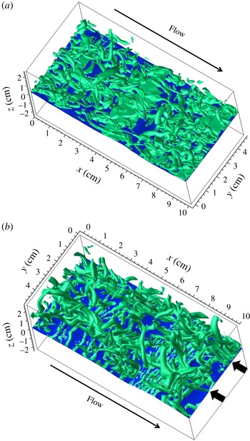
indicates stronger vortices. Figure 8 shows the instantaneous isosurfaces on both the gas and liquid sides, with high positive values of
 $M$
at
 $t=6.0$
s, where the isosurfaces on the liquid side are shown in the bottom view. The typical horseshoe vortices associated with bursting motions, which are similar to those over a flat rigid wall, can be observed. In addition, these typical horseshoe vortices on the liquid side seem to be concentrated at two locations indicated by thick arrows. This point will be discussed later.
Instantaneous isosurfaces of the second invariant,
 $M$
, on (a) the gas side and (b) the liquid side at
 $t=6.0$
s (the values of the isosurfaces are 500 and 128 s
 $^{-2}$
on the gas and liquid sides respectively). The thick arrows show the locations where horseshoe vortices are concentrated on the liquid side.

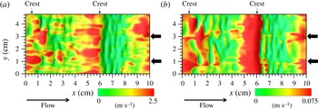
Distributions of instantaneous streamwise velocities (a) at
 $z_{G}^{+}=10$
on the gas side,
 $u_{G}(x,y,t)$
, and (b) at
 $z_{L}^{+}=-10$
on the liquid side,
 $u_{L}$
(
 $x,y,t$
), at
 $t=6.0$
s. The thick arrows indicate the same locations as in figure 8. The thin arrows indicate the positions of main wave crests.

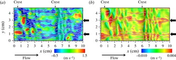
Distributions of instantaneous streamwise velocity fluctuations (a) at
 $z_{G}^{+}=10$
on the gas side,
 $u_{G}^{\prime \prime }(x,y,t)$
, and (b) at
 $z_{L}^{+}=-10$
on the liquid side,
 $u_{L}^{\prime \prime }(x,y,t)$
, at
 $t=6.0$
s. The white dots show the locations of local minimum values in the spanwise direction. The thick arrows indicate the same locations as in figure 8. The thin arrows indicate the positions of main wave crests.

Figure 9 shows the distributions of the instantaneous streamwise velocities on the gas side at
 $z_{G}^{+}=10$
,
 $u_{G}(x,y,t)$
, and on the liquid side at
 $z_{L}^{+}=-10$
,
 $u_{L}(x,y,t)$
, at
 $t=6.0$
s. It is observed that low- and high-velocity streaks appear on the gas and liquid sides respectively. To quantitatively investigate the streak properties, the spacing of the low-velocity streaks on the gas flow and that of the high-velocity streaks on the liquid flow were calculated by the following process. A variable,
 $f(x,y,t)$
, on the
 $x$
–
 $y$
plane was decomposed as
 $$\begin{eqnarray}\displaystyle f(x,y,t)=\langle f\rangle _{y}(x,t)+f^{\prime \prime }(x,y,t), & & \displaystyle\end{eqnarray}$$
where
 $\langle f\rangle _{y}(x,t)$
is the spanwise average over
 $y$
(e.g. Sullivan, McWilliams & Moeng Reference Sullivan, McWilliams and Moeng2000; Tsai et al.
Reference Tsai, Chen, Lu and Garbe2013) and
 $f^{\prime \prime }(x,y,t)$
is the fluctuation component. The local maximum (minimum) values of
 $f^{\prime \prime }(x,y,t)$
are used to define the centres of the velocity streaks having high (low) values of the variable,
 $f(x,y,t)$
respectively. Then, the velocity-streak spacing,
 $\unicode[STIX]{x1D706}$
(
 $t$
), is calculated as the spanwise distance between the centres of two velocity streaks. Figure 10 shows the distributions of the instantaneous streamwise velocity fluctuations on the gas side at
 $z_{G}^{+}=10$
,
 $u_{G}^{\prime \prime }(x,y,t)$
, and on the liquid side at
 $z_{L}^{+}=-10$
,
 $u_{L}^{\prime \prime }(x,y,t)$
, at
 $t=6.0$
s. In the figure, white dots indicating locations with the local minimum and maximum values for
 $u_{G}^{\prime \prime }(x,y,t)$
and
 $u_{L}^{\prime \prime }(x,y,t)$
are superimposed. The dots illustrate the low-velocity and high-velocity streaks on each side more clearly, and hence these dots can be used for estimating the streak spacing.
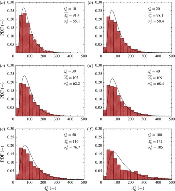
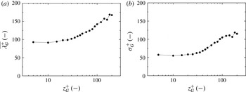
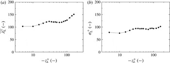
Figure 11 shows the probability density function (PDF) distributions of the velocity-streak spacing on the gas side,
 $\unicode[STIX]{x1D706}_{G}^{+}$
, at
 $z_{G}^{+}=10$
, 20, 30, 40, 50 and 100 and figure 12 shows those on the liquid side,
 $\unicode[STIX]{x1D706}_{L}^{+}$
, at
 $z_{L}^{+}=-10$
,
 $-20$
,
 $-30$
,
 $-40$
,
 $-50$
and
 $-100$
. Here,
 $\unicode[STIX]{x1D706}_{G}^{+}$
and
 $\unicode[STIX]{x1D706}_{L}^{+}$
are normalized by the friction velocities,
 $u_{G}^{\ast }$
and
 $u_{L}^{\ast }$
, and viscosities,
 $\unicode[STIX]{x1D708}_{G}$
and
 $\unicode[STIX]{x1D708}_{L}$
, on the liquid and gas sides respectively. In figure 11 for the gas side, the normalized mean value (
 $\overline{\unicode[STIX]{x1D706}_{G}^{+}}=91$
at
 $z_{G}^{+}=10$
) and its standard deviation (
 $\unicode[STIX]{x1D70E}_{G}^{+}=55$
at
 $z_{G}^{+}=10$
) are close to those in the wall turbulent boundary layer (
 $\overline{\unicode[STIX]{x1D706}^{+}}=80{-}120$
and
 $\unicode[STIX]{x1D70E}^{+}/\overline{\unicode[STIX]{x1D706}^{+}}=0.3{-}0.4$
, Kline et al.
Reference Kline, Reynolds, Schraub and Runstadler1967;
 $\overline{\unicode[STIX]{x1D706}^{+}}=93{-}105$
and
 $\unicode[STIX]{x1D70E}^{+}=36{-}47$
, Smith & Metzler Reference Smith and Metzler1983) and tend to increase with increasing
 $z_{G}^{+}$
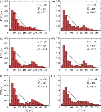
. In figure 12 for the liquid side, on the other hand, while the normalized mean velocity-streak spacing (
 $\overline{\unicode[STIX]{x1D706}_{L}^{+}}=103$
at
 $z_{L}^{+}=-10$
) is in the same range as in the wall turbulent boundary layer, the normalized standard deviation (
 $\unicode[STIX]{x1D70E}_{L}^{+}=76$
at
 $z_{L}^{+}=-10$
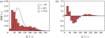
) is larger than that in the wall turbulent boundary layer. In addition, a second peak appears in the PDF of
 $\overline{\unicode[STIX]{x1D706}_{L}^{+}}$
far from the gas–liquid interface (
 $z_{L}^{+}=-20$
to
 $-100$
). It is considered that this is caused by Langmuir circulations (Takagaki et al.
Reference Takagaki, Kurose, Tsujimoto, Komori and Takahashi2015), which are illustrated in terms of the second invariant indicated by two thick arrows in figure 8(b). The details will be discussed below. Figures 13 and 14 show the vertical distributions of
 $\overline{\unicode[STIX]{x1D706}^{+}}$
and
 $\unicode[STIX]{x1D70E}^{+}$
on both the gas and liquid sides respectively. There are near-interface layers taking constant values of
 $\overline{\unicode[STIX]{x1D706}^{+}}$
and
 $\unicode[STIX]{x1D70E}^{+}$
on the gas and liquid sides respectively at
 $0<z_{G}^{+}<10$
and
 $-10<z_{L}^{+}<0$
; these trends are consistent with those in the wall turbulent boundary layer (
 $z^{+}=1{-}10$
) (Smith & Metzler Reference Smith and Metzler1983).
The PDFs of the velocity-streak spacing,
 $\unicode[STIX]{x1D706}_{G}^{+}$
, at
 $z_{G}^{+}=10$
, 20, 30, 40, 50 and 100 (a–f) on the gas side at
 $t=6.0$
s. Here,
 $\unicode[STIX]{x1D706}_{G}^{+}$
is normalized by the friction velocity,
 $u_{G}^{\ast }$
, and viscosity,
 $\unicode[STIX]{x1D708}_{G}$
, on the gas side. The bin width is set to be
 $\unicode[STIX]{x1D706}_{G}^{+}=25$
. The terms
 $\overline{\unicode[STIX]{x1D706}_{G}^{+}}$
and
 $\unicode[STIX]{x1D70E}_{G}^{+}$
are the normalized mean values and standard deviations of
 $\unicode[STIX]{x1D706}_{G}^{+}$
respectively. The lines show the log-normal distribution at each
 $\overline{\unicode[STIX]{x1D706}_{G}^{+}}$
and
 $\unicode[STIX]{x1D70E}_{G}^{+}$
. The PDFs are obtained by taking the time average of
 $t=5.75$
–6.25 s.

The PDFs of the velocity-streak spacing,
 $\unicode[STIX]{x1D706}_{L}^{+}$
, at
 $z_{L}^{+}=-10$
,
 $-20$
,
 $-30$
,
 $-40$
,
 $-50$
and
 $-100$
(a–f) on the liquid side at
 $t=6.0$
s. Here,
 $\unicode[STIX]{x1D706}_{L}^{+}$
is normalized by the friction velocity,
 $u_{L}^{\ast }$
, and viscosity,
 $\unicode[STIX]{x1D708}_{L}$
, on the liquid side. The bin width is set to be
 $\unicode[STIX]{x1D706}_{L}^{+}=19$
. The terms
 $\overline{\unicode[STIX]{x1D706}_{L}^{+}}$
and
 $\unicode[STIX]{x1D70E}_{L}^{+}$
are normalized mean values and standard deviations of
 $\unicode[STIX]{x1D706}_{L}^{+}$
respectively. The lines show the log-normal distribution at each
 $\overline{\unicode[STIX]{x1D706}_{L}^{+}}$
and
 $\unicode[STIX]{x1D70E}_{L}^{+}$
. The PDFs are obtained by taking the time average of
 $t=5.75$
–6.25 s.

Vertical distributions of (a) the normalized mean value,
 $\overline{\unicode[STIX]{x1D706}_{G}^{+}}$
, and (b) the normalized standard deviation,
 $\unicode[STIX]{x1D70E}_{G}^{+}$
, of the velocity-streak spacing on the gas side at
 $t=6.0$
s. These values are obtained by taking the time average of
 $t=5.75$
–6.25 s.

Vertical distributions of (a) the normalized mean value,
 $\overline{\unicode[STIX]{x1D706}_{L}^{+}}$
, and (b) the normalized standard deviation,
 $\unicode[STIX]{x1D70E}_{L}^{+}$
, of the velocity-streak spacing on the liquid side at
 $t=6.0$
s. These values are obtained by taking the time average of
 $t=5.75$
–6.25 s.

Cross-sectional (
 $y$
–
 $z$
plane) distributions of streamwise-averaged values of (a) streamwise velocity,
 $\dot{u}$
, (b) spanwise velocity,
 $\dot{v}$
, (c) vertical velocity,
 ${\dot{w}}$
, and (d) streamwise vorticity,
 ${\dot{r}}_{32}$
, on the liquid side below the gas–liquid interface at
 $t=6.0$
s. The thick arrows show the locations of strong downward flows.

Cross-sectional (
 $y$
–
 $z$
plane) distributions of streamwise-averaged values of (a) streamwise velocity,
 $\dot{u}$
, (b) spanwise velocity,
 $\dot{v}$
, (c) vertical velocity,
 ${\dot{w}}$
, and (d) streamwise vorticity,
 ${\dot{r}}_{32}$
, on the gas side at
 $t=6.0$
s.

The PDFs of the high-velocity-streak spacing on the liquid side: (a) original PDF with log-normal distribution (line); (b) subtracted PDF at
 $t=6.0$
s. The PDFs are obtained by taking the time average of
 $t=5.75$
–6.25 s.

Many previous studies have mentioned streaks of Langmuir circulations appearing on gas–liquid interfaces, such as the streaks produced by oil, leaves, bubbles and small glass microspheres (Langmuir Reference Langmuir1938; Melville, Shear & Veron Reference Melville, Shear and Veron1998), surface scalar concentration (Takagaki et al.
Reference Takagaki, Kurose, Tsujimoto, Komori and Takahashi2015) and surface temperature (Schnieders et al.
Reference Schnieders, Garbe, Peirson, Smith and Zappa2013; Tsai et al.
Reference Tsai, Chen, Lu and Garbe2013). However, few researchers have discussed them in terms of the interaction of the underwater turbulent structures and second flows of Langmuir circulations. In general, the streak spacings of Langmuir circulations (
 $\unicode[STIX]{x1D706}_{LC}=0.033{-}280$
m; Assaf, Gerard & Gordon Reference Assaf, Gerard and Gordon1971; Melville et al.
Reference Melville, Shear and Veron1998) are much larger than those of turbulent vortices (
 $\unicode[STIX]{x1D706}_{T}=0.0001{-}0.01$
m in the range of
 $u_{L}^{\ast }=0.01{-}1.0~\text{m}~\text{s}^{-1}$
at
 $\unicode[STIX]{x1D708}_{L}=10^{-6}~\text{m}^{2}~\text{s}^{-1}$
and
 $\overline{\unicode[STIX]{x1D706}^{+}}=100$
), and hence the concentration of horseshoe vortices (figure 8
b) and the distribution of high-velocity streaks (figure 10
b) are considered to be caused by both Langmuir circulations and turbulent vortices on the liquid side. Recently, Tsai et al. (Reference Tsai, Chen, Lu and Garbe2013) and Takagaki et al. (Reference Takagaki, Kurose, Tsujimoto, Komori and Takahashi2015) evaluated the streak spacing of Langmuir circulations from the spacing of underwater downward flows using the streamwise-averaging method proposed by Tsai et al. (Reference Tsai, Chen, Lu and Garbe2013). Using this method, Langmuir circulations can be visualized by making a streamwise-averaging manipulation,
 $$\begin{eqnarray}\displaystyle \dot{\unicode[STIX]{x1D6F7}}=\frac{1}{4\unicode[STIX]{x1D6FF}}\int _{0}^{4\unicode[STIX]{x1D6FF}}\unicode[STIX]{x1D6F7}\,\text{d}x, & & \displaystyle\end{eqnarray}$$
against the physical variables,
 $\unicode[STIX]{x1D6F7}$
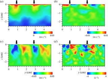
, with the turbulent flow fields containing both turbulent eddies and Langmuir circulations to remove the effect of turbulent eddies on the variables. Figure 15 shows the cross-sectional (
 $y$
–
 $z$
plane) distributions of the streamwise-averaged streamwise velocity,
 $\dot{u}$
, spanwise velocity,
 $\dot{v}$
, vertical velocity,
 ${\dot{w}}$
, and streamwise vorticity,
 ${\dot{r}}_{32}$
, on the liquid side below the gas–liquid interface at
 $t=6.0$
s. Two solitary parts with strong downstream flow (positive
 $\dot{u}$
) just below the gas–liquid interface can be seen accompanying the strong downward flow (negative
 ${\dot{w}}$
) and pairs of strong vortices (positive and negative
 ${\dot{r}}_{32}$
). It is also confirmed that two solitary parts accompany the fast surface currents. To make the explanation clear, thick arrows are added to indicate the strong downward flows in the figure. Leibovich (Reference Leibovich1983) and Thorpe (Reference Thorpe2004) pointed out that Langmuir circulations accompany strong streamwise surface currents and downward flows on the liquid side, whose trends match well with the present predicted ones. The present streak spacing of Langmuir circulations is roughly evaluated to be
 $\unicode[STIX]{x1D706}_{LC}=0.021$
m (
 $\unicode[STIX]{x1D706}_{LC,L}^{+}=268$
), where
 $\unicode[STIX]{x1D706}_{LC,L}^{+}$
is
 $\unicode[STIX]{x1D706}_{LC}$
normalized by
 $u_{L}^{\ast }$
and
 $\unicode[STIX]{x1D708}_{L}$
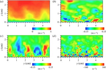
. On the other hand, figure 16 shows the cross-sectional (
 $y$
–
 $z$
plane) distributions of the streamwise-averaged streamwise velocity,
 $\dot{u}$
, spanwise velocity,
 $\dot{v}$
, vertical velocity,
 ${\dot{w}}$
, and streamwise vorticity,
 ${\dot{r}}_{32}$
, on the gas side above the gas–liquid interface at
 $t=6.0$
s. It is confirmed that secondary flow due to Langmuir circulation is hardly generated.
In this study, to qualitatively evaluate the streak spacing of Langmuir circulations on the liquid side, a new evaluation method using the PDF of high-velocity streaks on the liquid side and a log-normal distribution is proposed, and then the estimated values are compared with those of the high-velocity-streak spacing obtained from the streamwise-averaging method (Tsai et al.
Reference Tsai, Chen, Lu and Garbe2013) and the present method (referred to as the ‘subtracted-PDF method’ hereafter). Although the PDF of the high-velocity-streak spacing in the wind-wave turbulent field on the liquid side shows a log-normal distribution similar to the PDF of the low-velocity-streak spacing in the wall turbulent boundary layer, it is modulated by Langmuir circulations. In the subtracted-PDF method, this trend is taken into account to quantitatively evaluate the modulation due to Langmuir circulations. In figure 17, the original PDF distribution and the modulated PDF distribution, which is subtracted by the log-normal distribution with
 $\overline{\unicode[STIX]{x1D706}^{+}}=100$
and
 $\unicode[STIX]{x1D70E}^{+}=40$
, in the wind-wave turbulent field on the liquid side at
 $z_{L}^{+}=-10$
are shown. It is found that the subtracted PDF is separated into three bodies such that the summation of the subtracted PDF against
 $\unicode[STIX]{x1D706}_{L}^{+}$
is 0, and that the left and right bodies are generated by the modulation due to Langmuir circulations, and the centre body takes a negative value. Therefore, we define the normalized streak spacing of Langmuir circulations,
 $\unicode[STIX]{x1D706}_{LC,L}^{+}$
, as the mean spacing of the right body in the subtracted PDF. According to this method, the present streak spacing of Langmuir circulations is
 $\unicode[STIX]{x1D706}_{LC,L}^{+}=237$
(
 $\unicode[STIX]{x1D706}_{LC}=0.019$
m).
As mentioned above, it is considered that Langmuir circulation causes streaks of oil, leaves, bubbles and small glass microspheres (Langmuir Reference Langmuir1938; Melville et al.
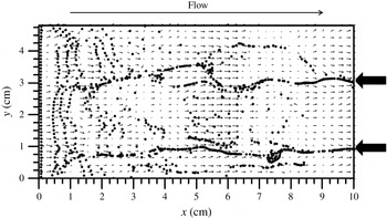
Reference Melville, Shear and Veron1998) on gas–liquid interfaces. Hence, we examine the behaviour of marker particles on the gas–liquid interface. Figure 18 shows the instantaneous distributions of the marker particles and velocity vectors on the gas–liquid interface at
 $t=6.0$
s. Here, the marker particles are initially aligned in the spanwise direction at equal distances along the line
 $x=0$
and
 $z=0$
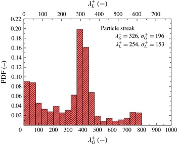
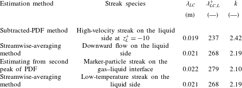
m, and tracked along the interface without imposing periodic boundary conditions in the streamwise direction. That is, the locations of the instantaneous particles are determined by their instantaneous tangential velocities on the free surface, and this implies that the particles cannot leave the free surface. The marker particles tend to form fewer streaks at the same locations as Langmuir circulations with time (figures 8(b), 10(b) and 15). Figure 19 shows the PDF distribution of the marker-particle-streak spacing. The streak spacing of Langmuir circulations,
 $\unicode[STIX]{x1D706}_{LC}$
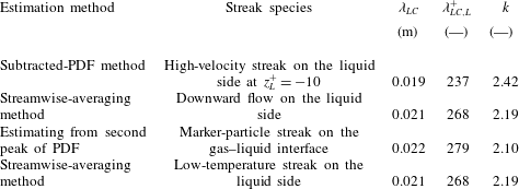
, is regarded as the second peak of the PDF of the marker-particle-streak spacing, and is estimated to be 0.022 m. This is listed in table 2, together with those by the flow behaviour obtained by using the subtracted-PDF (
 $\unicode[STIX]{x1D706}_{LC}=0.019$
m) and streamwise-averaging methods (
 $\unicode[STIX]{x1D706}_{LC}=0.021$
m), as explained above. It is found that the values of
 $\unicode[STIX]{x1D706}_{LC}$
obtained by these methods agree with each other. Thus, we have succeeded in reproducing the phenomenon that the marker-particle streaks are induced by Langmuir circulations.


The PDFs of the marker-particle-streak spacing at
 $t=6.0$
s. These values are obtained by taking the time average of
 $t=5.75-6.25$
s. The bin width is set to be
 $\unicode[STIX]{x1D706}_{G}^{+}=40$
and
 $\unicode[STIX]{x1D706}_{L}^{+}=31$
.

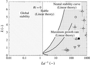
The neutral stability theory by Leibovich & Paolucci (Reference Leibovich and Paolucci1981) with present and previous data: ▪, present (DNS); ○, Tsai et al. (Reference Tsai, Chen, Lu and Garbe2013) (DNS); ▫, Melville et al. (Reference Melville, Shear and Veron1998) (laboratory); ▵, Schnieders et al. (Reference Schnieders, Garbe, Peirson, Smith and Zappa2013) (laboratory); ▿, Takagaki et al. (Reference Takagaki, Kurose, Tsujimoto, Komori and Takahashi2015) (DNS). The present value is evaluated by the streamwise-averaging method.

Predicted characteristics of Langmuir circulations at
 $t=6.0$
s and
 $U_{\infty }=4.0~\text{m}~\text{s}^{-1}$
. The Langmuir number,
 $La$
, is 0.00328 for all cases. Here,
 $\unicode[STIX]{x1D706}_{LC}$
is the streak spacing of Langmuir circulations,
 $\unicode[STIX]{x1D706}_{LC,L}^{+}$
is
 $\unicode[STIX]{x1D706}_{LC}$
normalized by the friction velocity and viscosity on the liquid side, and
 $k$
is the normalized transverse wavenumber of Langmuir circulations based on
 $\unicode[STIX]{x1D706}_{LC}$
.
Finally, to theoretically predict whether Langmuir circulations could emerge or not, a stability diagram proposed by Leibovich & Paolucci (Reference Leibovich and Paolucci1981), which shows the relation between the inverse Langmuir number,
 $La^{-1}$
, and the normalized transverse wavenumber based on the streak spacing of Langmuir circulations,
 $k$
, is introduced (figure 20). These terms are defined as follows:
 $$\begin{eqnarray}\displaystyle & \displaystyle La=\left(\frac{\unicode[STIX]{x1D708}_{L,t}^{3}k_{S}^{2}}{\unicode[STIX]{x1D714}a^{2}u_{L}^{\ast 2}}\right)^{1/2}, & \displaystyle\end{eqnarray}$$
 $$\begin{eqnarray}\displaystyle & \displaystyle k=\frac{k_{Langmuir}}{k_{S}}, & \displaystyle\end{eqnarray}$$
 $\unicode[STIX]{x1D708}_{L,t}$
is the eddy viscosity on the liquid side,
 $k_{S}$
is the wavenumber of significant wind waves (
 $k_{S}=2\unicode[STIX]{x03C0}/L_{S}$
),
 $\unicode[STIX]{x1D714}$
is the significant wave angular frequency (
 $\unicode[STIX]{x1D714}=2\unicode[STIX]{x03C0}/T_{S}$
),
 $a$
is the wave amplitude (
 $a=H_{S}/2$
),
 $u_{L}^{\ast }$
is the friction velocity on the liquid side and
 $k_{Langmuir}$
is the dimensional wavenumber based on the streak spacing of Langmuir circulations. Here,
 $\unicode[STIX]{x1D708}_{L,t}$
is estimated by using the empirical equation proposed by Ichiye (Reference Ichiye1967) in the same manner as Huang (Reference Huang1979) and Tsai et al. (Reference Tsai, Chen, Lu and Garbe2013). According to these definitions, the present
 $La^{-1}$
is 305, and
 $k$
is 2.19 (by the streamwise-averaging method) and 2.42 (by the subtracted-PDF method). In addition, for the previously measured spacing of the marker-particle streaks,
 $\unicode[STIX]{x1D706}_{LC}$
(Melville et al.
Reference Melville, Shear and Veron1998, table I), ranging from 3.3 to 7.5 cm, the friction velocity on the liquid side (
 $u_{L}^{\ast }=0.38{-}0.81~\text{cm}~\text{s}^{-1}$
) is estimated using the empirical relation (Komori, Nagaosa & Murakami Reference Komori, Nagaosa and Murakami1993b
)
 $$\begin{eqnarray}\displaystyle u_{G}^{\ast }=0.02U_{\infty }^{1.5} & & \displaystyle\end{eqnarray}$$
and the relation
 $$\begin{eqnarray}\displaystyle \unicode[STIX]{x1D70F}=\unicode[STIX]{x1D70C}_{G}u_{G}^{\ast 2}=\unicode[STIX]{x1D70C}_{L}u_{L}^{\ast 2}. & & \displaystyle\end{eqnarray}$$
This figure certainly confirms the appearance of Langmuir circulations in the stability diagram in the present and previous studies (Melville et al. Reference Melville, Shear and Veron1998; Schnieders et al. Reference Schnieders, Garbe, Peirson, Smith and Zappa2013; Tsai et al. Reference Tsai, Chen, Lu and Garbe2013; Takagaki et al. Reference Takagaki, Kurose, Tsujimoto, Komori and Takahashi2015).
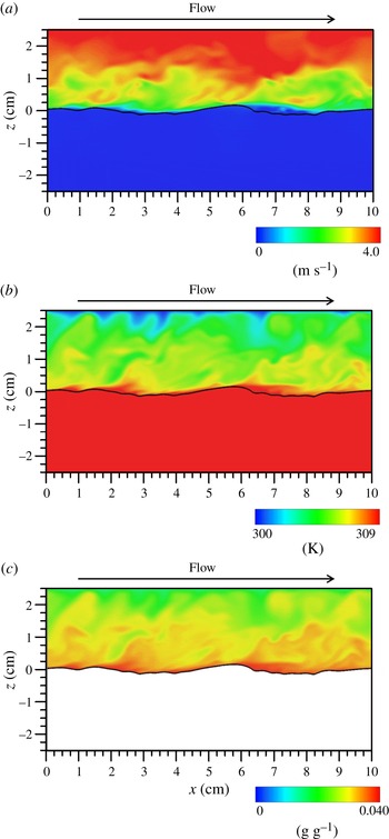
Instantaneous distributions of (a) streamwise velocity on the gas and liquid sides, (b) temperature on the gas and liquid sides, and (c) specific humidity only on the gas side on the
 $x$
–
 $z$
plane at
 $y=0.024$
m and
 $t=6.0$
s. The lines show the instantaneous gas–liquid interface.

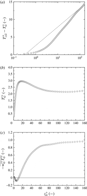
Vertical distributions of (a) normalized mean temperature,
 $T_{i,G}^{+}-T_{G}^{+}$
, (b) temperature fluctuation,
 $T_{G}^{\prime +}$
, and (c) vertical convective heat flux,
 $-\overline{w_{G}^{\prime +}T_{G}^{\prime +}}$
, on the gas side at
 $t=6.0$
s. The dashed line in (a) shows the log law calculated using (3.24). These values are obtained by taking the time average of
 $t=5.75$
–6.25 s and space average in the streamwise and spanwise directions.

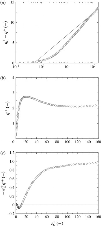
Vertical distributions of (a) normalized mean specific humidity,
 $q_{i}^{+}-q^{+}$
, (b) specific-humidity fluctuation,
 $q^{\prime +}$
, and (c) vertical specific-humidity flux,
 $-\overline{w^{\prime +}q^{\prime +}}$
, at
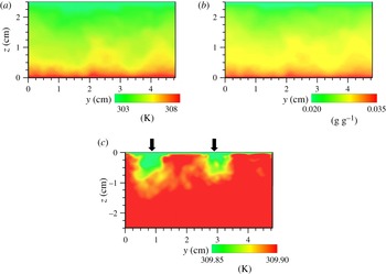
 $t=6.0$
s. The dashed line in (a) shows the log law calculated using (3.25). These values are obtained by taking the time average of
 $t=5.75$
–6.25 s and space average in the streamwise and spanwise directions.

3.3 Temperature and moisture fields
Figure 21 shows the instantaneous distributions of the streamwise velocity, temperature and specific humidity on the
 $x$
–
 $z$
plane at
 $y=0.024$
m and
 $t=6.0$
s. The distribution of the specific humidity is given only on the gas side. It is observed that low-wind-speed separated flows on the gas side exist on the leeward side of wind waves, and separated flows exist with high-temperature and high-specific-humidity conditions. Figure 22 shows the vertical distributions of the mean temperature,
 $T_{i,G}^{+}-T_{G}^{+}$
, temperature fluctuation,
 $T_{G}^{\prime +}$
, and vertical convective heat flux,
 $-\overline{w_{G}^{\prime +}T_{G}^{\prime +}}$
, on the gas side. Here,
 $T_{i}$
is the surface temperature, and this temperature is normalized by the friction temperature on the gas side,
 $T_{G}^{\ast }$
, which was estimated by
 $$\begin{eqnarray}\displaystyle T_{G}^{\ast }=\frac{\langle Q_{H}\rangle _{xy}}{\unicode[STIX]{x1D70C}_{G}C_{p,G}u_{G}^{\ast }}, & & \displaystyle\end{eqnarray}$$
where
 $\langle Q_{H}\rangle _{xy}$
is the sensible heat flux averaged over
 $x$
and
 $y$
at
 $z=0$
m. Further, figure 23 shows the vertical distributions of the mean specific humidity,
 $q_{i}^{+}-q^{+}$
, specific-humidity fluctuation,
 $q^{\prime +}$
, and vertical specific-humidity flux,
 $-\overline{w^{\prime +}q^{\prime +}}$
. Here,
 $q_{i}$
is the surface specific humidity, and the specific humidity including
 $q_{i}$
is normalized by the friction specific humidity,
 $q^{\ast }$
, which is estimated by
 $$\begin{eqnarray}\displaystyle q^{\ast }=\frac{\langle Q_{E}\rangle _{xy}}{\unicode[STIX]{x1D70C}_{G}L_{V}u_{G}^{\ast }}. & & \displaystyle\end{eqnarray}$$
Additionally, the lines in figures 22(a) and 23(a) are described by
 $$\begin{eqnarray}\displaystyle & \displaystyle T_{i}-T(z)=\frac{Pr_{t}T_{G}^{\ast }}{\unicode[STIX]{x1D705}}\ln \frac{z}{z_{0T}}, & \displaystyle\end{eqnarray}$$
 $$\begin{eqnarray}\displaystyle & \displaystyle q_{i}-q(z)=\frac{Sc_{t}q^{\ast }}{\unicode[STIX]{x1D705}}\ln \frac{z}{z_{0q}}. & \displaystyle\end{eqnarray}$$
 $Pr_{t}$
(
 $=\unicode[STIX]{x1D708}_{Gt}/\unicode[STIX]{x1D6FC}_{Gt}$
, where
 $\unicode[STIX]{x1D708}_{Gt}$
is the eddy viscosity on the gas side and
 $\unicode[STIX]{x1D6FC}_{Gt}$
is the eddy thermal diffusivity on the gas side) is the turbulent Prandtl number,
 $z_{0t}$
is the roughness length for the given temperature,
 $Sc_{t}$
(
 $=\unicode[STIX]{x1D708}_{Gt}/D_{t}$
, where
 $\unicode[STIX]{x1D708}_{Gt}$
is the eddy viscosity on the gas side and
 $D_{t}$
is the eddy diffusivity of moisture on the gas side) is the turbulent Schmidt number for the specific humidity and
 $z_{0q}$
is the roughness length for the specific humidity. The buoyancy effects are negligibly small in the present case (see § 3.1). The constant values, i.e.
 $Pr_{t}=0.915$
and
 $Sc_{t}=0.918$
, are estimated from
 $$\begin{eqnarray}\displaystyle & \displaystyle Pr_{t}=\frac{-\overline{u^{\prime }w^{\prime }}\displaystyle \frac{\text{d}T}{\text{d}z}}{\overline{w^{\prime }T^{\prime }}\displaystyle \frac{\text{d}U}{\text{d}z}}, & \displaystyle\end{eqnarray}$$
 $$\begin{eqnarray}\displaystyle & \displaystyle Sc_{t}=\frac{-\overline{u^{\prime }w^{\prime }}\displaystyle \frac{\text{d}q}{\text{d}z}}{\overline{w^{\prime }q^{\prime }}\displaystyle \frac{\text{d}U}{\text{d}z}}. & \displaystyle\end{eqnarray}$$
 $T_{i,G}^{+}-T_{G}^{+}$
and
 $q_{i}^{+}-q^{+}$
are found to follow log laws, whereas
 $T_{G}^{\prime +}$
,
 $-\overline{w_{G}^{\prime +}T_{G}^{\prime +}}$
,
 $q^{\prime +}$
and
 $-\overline{w^{\prime +}q^{\prime +}}$
tend to saturate around
 $z_{G}^{+}=100\sim 160$
, because of the numerical upper boundary condition (the Dirichlet condition) for temperature and specific humidity. The negative peaks of
 $-\overline{w_{G}^{\prime +}T_{G}^{\prime +}}$
and
 $-\overline{w^{\prime +}q^{\prime +}}$
near the gas–liquid interface originate from the wake on the leeward side of wind waves similarly to the Reynolds stress.
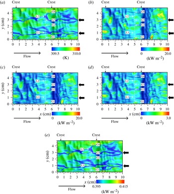
Surface distributions of instantaneous (a) temperature,
 $T_{i}$
, (b) total heat flux,
 $Q_{T}$
, (c) latent heat flux,
 $Q_{E}$
, (d) sensible heat flux,
 $Q_{H}$
, and (e) radiative heat flux,
 $Q_{R}$
, at
 $t=6.0$
s. The thick arrows indicate the same locations as in figures 8–10. The arrows G1–G4 show the locations of upward flows on the gas side (figure 25
a–c), whereas the arrows L1 and L2 show the locations of downward flows on the liquid side (figure 25
d,e). The dotted lines show
 $x=0.05$
m, which corresponds to the location of the plane in figure 25. The thin arrows indicate the positions of main wave crests.

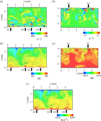
Instantaneous distributions of (a) streamwise vorticity on the gas side, (b) temperature on the gas side, (c) specific humidity on the gas side, (d) streamwise vorticity on the liquid side and (e) temperature on the liquid side on the
 $y$
–
 $z$
plane at
 $x=0.05$
m and
 $t=6.0$
s. Each bottom boundary shows the instantaneous gas–liquid interface. In (a) and (d), the positive and negative areas indicate the locations having counterclockwise and clockwise vorticities respectively. The velocity vectors are inscribed in all of the figures. The thick arrows G1–G4 show the locations of upward flows on the gas side, and the thick arrows L1 and L2 show the locations of downward flows on the liquid side.

Figure 24 shows the surface distributions of the instantaneous temperature,
 $T_{i}$
, total heat flux,
 $Q_{T}$
, latent heat flux,
 $Q_{E}$
, sensible heat flux,
 $Q_{H}$
, and radiative heat flux,
 $Q_{R}$
, at
 $t=6.0$
s. Here, the local
 $Q_{T}$
,
 $Q_{E}$
,
 $Q_{H}$
and
 $Q_{R}$
are defined by (2.10)–(2.13) respectively. To visualize the distribution of the heat flux clearly, the ranges of the colour contours are made different for each flux. In the figure, the locations indicated by arrows G1–G4, L1 and L2 correspond to those indicated by the thick arrows with the same symbols in figure 25, which are determined by the temperature fields on the gas and liquid sides, as explained below. The low-heat-flux areas are located on the leeward side (
 $x=0.06\sim 0.07$
m) of the wind waves for
 $Q_{T}$
,
 $Q_{E}$
and
 $Q_{H}$
. This is because the separated flows (see figure 21) generated on the gas side of the leeward side of the wind wave tend to stagnate the high-temperature and high-specific-humidity fluid, which suppresses the heat transfer across the gas–liquid interface. On the other hand, such an effect of the separated flows (see figure 21) on the gas side cannot be seen for
 $T_{i}$
and
 $Q_{R}$
. This observation and the fact that radiative heat transfer from the gas–liquid interface is mainly controlled by the surface temperature suggest that
 $T_{i}$
is not affected by the turbulent eddies on the gas side as much as
 $Q_{T}$
,
 $Q_{E}$
and
 $Q_{H}$
. It is also observed that the streamwise low-
 $T_{i}$
streaks and low-heat-flux streaks of
 $Q_{T}$
,
 $Q_{E}$
,
 $Q_{H}$
and
 $Q_{R}$
are similarly generated on the gas–liquid interface. To understand the generation mechanism of these streamwise streaks, the cross-sectional (
 $y$
–
 $z$
plane) distributions of the instantaneous streamwise vorticity with velocity vectors, temperature and specific humidity on the gas side, and those of the instantaneous streamwise vorticity with velocity vectors and temperature on the liquid side at
 $x=0.05$
m and at
 $t=6.0$
s are shown in figure 25. On the gas side (figure 25
a–c), upward flows are generated by pairs of turbulent eddies near the gas–liquid interface, and the regions with high temperature and high specific humidity are formed by the upward flows (indicated by arrows G1–G4), which means that the fluid heated at the gas–liquid interface is transferred by the upward flow on the gas side. On the contrary, on the liquid side (figure 25
d,e), downward flows are generated by pairs of turbulent eddies near the gas–liquid interface, and the low-temperature regions are formed by the downward flows (indicated by arrows L1, L2), which means that the fluid cooled at the gas–liquid interface is transferred by the downward flow on the liquid side. It is also found that the locations of these upward/downward bursting motions near the gas–liquid interface correspond to the locations of the low-
 $T_{i}$
streak and low-heat-flux streaks for
 $Q_{T}$
,
 $Q_{E}$
,
 $Q_{H}$
and
 $Q_{R}$
(indicated by arrows G1–G4, L1, L2 in figure 24). This relation is clearly explained in the paper by Komori et al. (Reference Komori, Kurose, Iwano, Ukai and Suzuki2010, figure 23), in which mass transfer is considered. Namely, the downward bursting motions on the liquid side increase the scalar thickness and then suppress the scalar transfer at these locations. The difference from the results in the study by Komori et al. (Reference Komori, Kurose, Iwano, Ukai and Suzuki2010) for the mass transfer is that the heat transfer targeted in this study is affected not only by the turbulent eddies on the liquid side but also by those on the gas side. The reason for the difference in the scalar transfer mechanism between the mass and heat transfers will be discussed in more detail in § 3.4.
As in the case of the flow field described in § 3.2, the spacing of the low-
 $T_{i}$
streaks and low-heat-flux streaks for
 $Q_{T}$
,
 $Q_{E}$
,
 $Q_{H}$
and
 $Q_{R}$
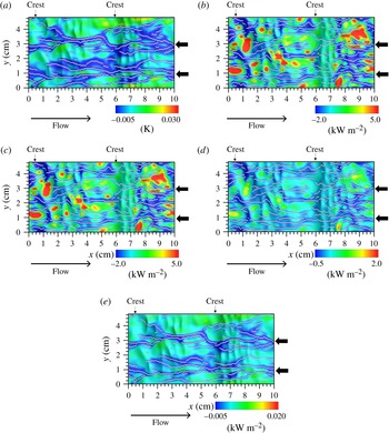
is investigated in more detail. The fluctuations of temperature,
 $T_{i}^{\prime \prime }$
(
 $x$
,
 $y$
,
 $t$
), and fluxes,
 $F^{\prime \prime }$
(
 $x$
,
 $y$
,
 $t$
), are calculated for locations having local minimum values for
 $T_{i}^{\prime \prime }$
(
 $x$
,
 $y$
,
 $t$
) and
 $F^{\prime \prime }$
(
 $x$
,
 $y$
,
 $t$
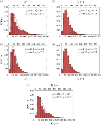
), as shown in figure 26, by the same detection method for the local minimum values as in figures 9 and 10. Further, figure 27 shows the PDF distributions of the low-
 $T_{i}$
streak and low-heat-flux streaks of
 $Q_{T}$
,
 $Q_{E}$
,
 $Q_{H}$
and
 $Q_{R}$
. Here,
 $\unicode[STIX]{x1D706}_{G}^{+}$
and
 $\unicode[STIX]{x1D706}_{L}^{+}$
are the normalized streak spacings of low-
 $T_{i}$
 $Q_{T}$
,
 $Q_{E}$
,
 $Q_{H}$
or
 $Q_{R}$
using the gas and liquid properties respectively, and
 $\unicode[STIX]{x1D706}_{G}^{+}$
and
 $\unicode[STIX]{x1D706}_{L}^{+}$
are their streak spacings. It is found that the PDF distributions for
 $Q_{T}$
,
 $Q_{E}$
and
 $Q_{H}$
correspond to log-normal distributions as with the distribution of the low-velocity-streak spacing on the wall turbulent boundary layer (Smith & Metzler Reference Smith and Metzler1983). However, their mean streak spacings (
 $\overline{\unicode[STIX]{x1D706}_{G}^{+}}=85.0$
, 85.1 and 84.0;
 $\overline{\unicode[STIX]{x1D706}_{L}^{+}}=66.3$
, 66.3 and 65.5 for
 $Q_{T}$
,
 $Q_{E}$
and
 $Q_{H}$
respectively) tend to be a little smaller than those for the low-velocity streaks on the gas side and the high-velocity streaks on the liquid side (
 $\overline{\unicode[STIX]{x1D706}_{G}^{+}}=91.4$
and
 $\overline{\unicode[STIX]{x1D706}_{L}^{+}}=103$
) (figures 11
a and 12
a at
 $z_{G}^{+}=10$
and
 $z_{L}^{+}=-10$
) and those in the wall turbulent boundary layer (
 $\overline{\unicode[STIX]{x1D706}^{+}}=80\sim 120$
(Kline et al.
Reference Kline, Reynolds, Schraub and Runstadler1967);
 $\overline{\unicode[STIX]{x1D706}^{+}}=93\sim 105$
(Smith & Metzler Reference Smith and Metzler1983)), although their standard deviations (
 $\unicode[STIX]{x1D70E}_{G}^{+}=48.1$
, 48.2 and 47.8;
 $\unicode[STIX]{x1D70E}_{L}^{+}=37.5$
, 37.5 and 37.2 for
 $Q_{T}$
,
 $Q_{E}$
and
 $Q_{H}$
respectively) are consistent with those in the wall turbulent boundary layer (
 $\overline{\unicode[STIX]{x1D706}^{+}}=80\sim 120$
,
 $\unicode[STIX]{x1D70E}^{+}/\overline{\unicode[STIX]{x1D706}^{+}}=0.3\sim 0.4$
(Kline et al.
Reference Kline, Reynolds, Schraub and Runstadler1967);
 $\unicode[STIX]{x1D70E}^{+}=36\sim 47$
(Smith & Metzler Reference Smith and Metzler1983)). This supports the above suggestion that the heat transfer across the gas–liquid interface is affected by the turbulent eddies on both the gas and liquid sides, and the fact that the deviations in the values from the streak velocity spacing are smaller for
 $\overline{\unicode[STIX]{x1D706}_{G}^{+}}$
than for
 $\overline{\unicode[STIX]{x1D706}_{L}^{+}}$
implies that the effect of the turbulent eddies on the gas side is dominant. The details will be discussed in § 3.4.
Surface distributions of instantaneous fluctuations for (a) temperature,
 $T_{i}^{\prime \prime }$
, (b) total heat flux,
 $Q_{T}^{\prime \prime }$
, (c) latent heat flux,
 $Q_{E}^{\prime \prime }$
, (d) sensible heat flux,
 $Q_{H}^{\prime \prime }$
, and (e) radiative heat flux,
 $Q_{R}^{\prime \prime }$
, at
 $t=6.0$
s. The white dots show the locations of local minimum values. The thick arrows indicate the same locations as in figures 8–10. The thin arrows indicate the positions of main wave crests.

The PDFs of spacing for (a) low-
 $T_{i}$
streaks, (b) low-
 $Q_{T}$
streaks, (c) low-
 $Q_{E}$
streaks, (d) low-
 $Q_{H}$
streaks and (e) low-
 $Q_{R}$
streaks on the gas–liquid interface at
 $t=6.0$
s. Here,
 $\unicode[STIX]{x1D706}_{G}^{+}$
and
 $\unicode[STIX]{x1D706}_{L}^{+}$
show the streak spacing normalized by parameters on the gas side (
 $u_{G}^{\ast }$
and
 $\unicode[STIX]{x1D708}_{G}$
) and parameters on the liquid side (
 $u_{L}^{\ast }$
and
 $\unicode[STIX]{x1D708}_{L}$
) respectively. Bin widths are
 $\unicode[STIX]{x1D706}_{G}^{+}=25$
and
 $\unicode[STIX]{x1D706}_{L}^{+}=19.5$
. The terms
 $\overline{\unicode[STIX]{x1D706}^{+}}$
and
 $\unicode[STIX]{x1D70E}^{+}$
are the normalized mean values and standard deviations respectively of streak spacing. The lines show the log-normal distributions described using each normalized mean value and standard deviation. These values are obtained by taking the time average of
 $t=5.75$
–6.25 s.

On the other hand, the PDF distributions for
 $T_{i}$
and
 $Q_{R}$
do not correspond to log-normal distributions. Moreover, although the normalized mean values (
 $\overline{\unicode[STIX]{x1D706}_{G}^{+}}=101$
and 102, and
 $\overline{\unicode[STIX]{x1D706}_{L}^{+}}=78.9$
and 79.8, for
 $T_{i}$
and
 $Q_{R}$
respectively) are within the range of
 $\overline{\unicode[STIX]{x1D706}^{+}}=80{-}120$
, the normalized standard deviations (
 $\unicode[STIX]{x1D70E}_{G}^{+}=66.3$
and 68.7, and
 $\unicode[STIX]{x1D70E}_{L}^{+}=51.7$
and 53.6, for
 $T_{i}$
and
 $Q_{R}$
respectively) are larger than those in the wall turbulent boundary layer (
 $\unicode[STIX]{x1D70E}^{+}=36{-}47$
) (Smith & Metzler Reference Smith and Metzler1983). Furthermore, there seem to be weak second peaks in the PDFs for
 $T_{i}$
and
 $Q_{R}$
induced by Langmuir circulation, which is the same as in the velocity field on the liquid side (figure 12
a). These facts suggest that although
 $T_{i}$
and
 $Q_{R}$
are affected by the turbulent eddies on both the gas and liquid sides, the effect of the turbulent eddies (including Langmuir circulations) on the liquid side is prominent. Further, this speculation is consistent with the above discussion on the separated flow effect on the heat transfer (figures 21 and 24). To further investigate the effects of Langmuir circulations on the temperature and moisture fields, the abovementioned streamwise-averaging method (Tsai et al.
Reference Tsai, Chen, Lu and Garbe2013) is applied to the temperature and specific-humidity fields. Figure 28 shows the cross-sectional (
 $y$
–
 $z$
plane) distributions of the streamwise-averaged values of temperature on the gas side, specific humidity on the gas side and temperature on the liquid side at
 $t=6.0$
s. The comparisons with the flow fields (figures 15 and 16) show that compared with the temperature and specific-humidity fields on the gas side, the temperature field on the liquid side is strongly affected by its flow field. In other words, two low-temperature regions on the liquid side, indicated by thick arrows (figure 28
c), are found to correspond to the two solitary parts formed by Langmuir circulations (figure 15). Judging from this temperature distribution on the liquid side, the low-temperature-streak spacing,
 $\unicode[STIX]{x1D706}_{LC,L}^{+}$
, is estimated to be 268 (
 $\unicode[STIX]{x1D706}_{LC}=0.021$
m) (table 2). This suggests that the streak spacing for the temperature field on the liquid side corresponds to that for the flow field on the liquid side, and is affected by Langmuir circulations. In this study, a new objective technique for evaluation of the streak spacing of Langmuir circulations, namely the subtracted-PDF method, is proposed in § 3.2. However, this method cannot be used here because the log-normal distribution cannot be given for the streaks affected by both gas and liquid flows.
Cross-sectional (
 $y$
–
 $z$
plane) distributions of (a) streamwise-averaged temperature on the gas side, (b) streamwise-averaged specific humidity on the gas side and (c) streamwise-averaged temperature on the liquid side at
 $t=6.0$
s. The thick arrows in (c) show the locations of low-temperature regions.

3.4 The difference between the mass and heat transfer mechanisms
The transfer mechanism of heat across the mobile wavy sheared gas–liquid interface is different from that of mass (e.g. Komori et al. Reference Komori, Kurose, Iwano, Ukai and Suzuki2010; Takagaki et al. Reference Takagaki, Kurose, Tsujimoto, Komori and Takahashi2015), because of the differences in the physical properties (e.g. solubility, diffusivity and viscosity). As pointed in figures 21 and 25, the heat transfer is affected by fluid flows on both the gas and liquid sides, although the mass transfer is affected only by fluid flows on the liquid side (Komori et al. Reference Komori, Kurose, Iwano, Ukai and Suzuki2010; Takagaki et al. Reference Takagaki, Kurose, Tsujimoto, Komori and Takahashi2015). The difference between the mass and heat transfer mechanisms can be explained as follows.
According to the double-film model proposed by Lewis & Whitman (Reference Lewis and Whitman1924), the mass flux across gas–liquid interface,
 $F$
, can be given as
 $$\begin{eqnarray}\displaystyle F=K_{G}(P_{BG}-P_{BL})=K_{L}(C_{BG}-C_{BL})=k_{G}(P_{BG}-P_{i})=k_{L}(C_{i}-C_{BL}), & & \displaystyle\end{eqnarray}$$
where
 $K_{G}$
is the overall mass transfer coefficient on the gas side (e.g. Bird, Stewart & Lightfoot Reference Bird, Stewart and Lightfoot1960),
 $P_{BG}$
is the bulk pressure of the mass on the gas side,
 $P_{BL}$
is the bulk pressure of the mass on the liquid side,
 $K_{L}$
is the overall mass transfer coefficient on the liquid,
 $C_{BG}$
is the bulk mass concentration on the gas side,
 $C_{BL}$
is the bulk mass concentration on the liquid side,
 $k_{G}$
is the mass transfer coefficient on the gas side,
 $P_{i}$
is the pressure of the mass at the gas–liquid interface,
 $k_{L}$
is the liquid-side mass transfer coefficient and
 $C_{i}$
is the mass concentration at the gas–liquid interface. Using Henry’s law, written as
 $C=SP$
(
 $S$
refers to solubility), (3.28) can be rewritten as
 $$\begin{eqnarray}\displaystyle F=\frac{K_{G}}{S}(C_{BG}-C_{BL})=K_{L}(C_{BG}-C_{BL})=\frac{k_{G}}{S}(C_{BG}-C_{i})=k_{L}(C_{i}-C_{BL}). & & \displaystyle\end{eqnarray}$$
Accordingly, the relation among the four mass transfer coefficients is obtained as
 $$\begin{eqnarray}\displaystyle \frac{S}{K_{G}}=\frac{1}{K_{L}}=\frac{1}{k_{L}}+\frac{S}{k_{G}}, & & \displaystyle\end{eqnarray}$$
using the resistance to mass transfers on the liquid side,
 $k_{L}^{-1}$
, and that on the gas side,
 $Sk_{G}^{-1}$
. The flux can be given as
 $$\begin{eqnarray}\displaystyle F=\left(\frac{1}{k_{L}}+\frac{S}{k_{G}}\right)^{-1}\{S(P_{BG}-P_{i})+(C_{i}-C_{BL})\}. & & \displaystyle\end{eqnarray}$$
Equations (3.30) and (3.31) mean that (i) there is additivity for the driving forces on both the gas and liquid sides and (ii) the efficiency of fluid motion on the gas and liquid sides near the gas–liquid interface and solubility on the overall mass transfer coefficient can be qualitatively estimated. For
 $\text{CO}_{2}$
gas transfer across the gas–liquid interface, the resistance to mass transfer on the liquid side,
 $k_{L}^{-1}$
, is approximately 20 times larger than that on the gas side,
 $Sk_{G}^{-1}$
, because of
 $S=39~\text{mol}~\text{m}^{-3}~\text{atm}^{-1}$
at
 $20\,^{\circ }\text{C}$
and generally
 $k_{G}k_{L}^{-1}=100{-}1000$
(Jahne & Haußecker Reference Jahne and Haußecker1998) under the condition of fully developed wind-driven turbulent field on both the gas and liquid sides and typically
 $k_{G}k_{L}^{-1}=150$
(Munz & Roberts Reference Munz, Roberts, Brutsaert and Jirka1984). This means that
 $\text{CO}_{2}$
gas transfer across the gas–liquid interface is strongly controlled by the fluid motion on the liquid side.
Heat transfer coefficients:
 $t$
is the elapsed time,
 $h_{L}$
is the total heat transfer coefficient,
 $k_{G}$
and
 $C_{EN}$
are the latent heat transfer coefficients,
 $h_{G}$
and
 $C_{HN}$
are the sensible heat transfer coefficients and
 $C_{KN}$
is the enthalpy transfer coefficient.

Similarly, the heat flux across the gas–liquid interface,
 $Q$
, can be given, only if the temperature field is considered (e.g. Jahne & Haußecker Reference Jahne and Haußecker1998), to keep the additivity for the driving forces on both the gas and liquid sides, as
 $$\begin{eqnarray}\displaystyle Q & = & \displaystyle \unicode[STIX]{x1D70C}_{G}C_{pG}H_{G}(T_{BG}-T_{BL})=\unicode[STIX]{x1D70C}_{L}C_{pL}H_{L}(T_{BG}-T_{BL})\nonumber\\ \displaystyle & = & \displaystyle \unicode[STIX]{x1D70C}_{G}C_{pG}h_{G}(T_{BG}-T_{i})=\unicode[STIX]{x1D70C}_{L}C_{pL}h_{L}(T_{i}-T_{BL}),\end{eqnarray}$$
where
 $\unicode[STIX]{x1D70C}_{G}$
is the density on the gas side,
 $C_{pG}$
is the specific heat at constant pressure on the gas side,
 $H_{G}$
is the overall heat transfer coefficient on the gas side,
 $T_{BG}$
is the bulk temperature on the gas side,
 $T_{BL}$
is the bulk temperature on the liquid side,
 $\unicode[STIX]{x1D70C}_{L}$
is the density on the liquid side,
 $C_{pL}$
is the specific heat at constant pressure on the liquid side,
 $H_{L}$
is the overall heat transfer coefficient on the liquid side,
 $h_{G}$
is the heat transfer coefficient on the gas side (sensible heat transfer coefficient),
 $T_{i}$
is the surface temperature and
 $h_{L}$
is the heat transfer coefficient on the liquid side (total heat transfer coefficient). Using the solubility for temperature (
 $S_{T}=\unicode[STIX]{x1D70C}L_{V}C_{pL}\unicode[STIX]{x1D70C}_{G}^{-1}C_{pG}^{-1}$
) analogously proposed by Jahne & Haußecker (Reference Jahne and Haußecker1998), (3.32) can be rewritten as
 $$\begin{eqnarray}\displaystyle \frac{Q}{\unicode[STIX]{x1D70C}_{L}C_{pL}}=\frac{H_{G}}{S_{T}}(T_{BG}-T_{BL})=H_{L}(T_{BG}-T_{BL})=\frac{h_{G}}{S_{T}}(T_{BG}-T_{i})=h_{L}(T_{i}-T_{BL}). & & \displaystyle\end{eqnarray}$$
Accordingly, the relation among the four heat transfer coefficients is obtained as
 $$\begin{eqnarray}\displaystyle \frac{S_{T}}{H_{G}}=\frac{1}{H_{L}}=\frac{1}{h_{L}}+\frac{S_{T}}{h_{G}}, & & \displaystyle\end{eqnarray}$$
using the resistance to heat transfer on the liquid side,
 $h_{L}^{-1}$
, and that on the gas side,
 $S_{T}h_{G}^{-1}$
. The flux can be given as
 $$\begin{eqnarray}\displaystyle \frac{Q}{\unicode[STIX]{x1D70C}_{L}C_{pL}}=\left(\frac{1}{h_{L}}+\frac{S_{T}}{h_{G}}\right)^{-1}\{(T_{BG}-T_{i})+(T_{i}-T_{BL})\}. & & \displaystyle\end{eqnarray}$$
The heat transfer coefficient on the liquid side,
 $h_{L}$
, and heat transfer coefficient on the gas side,
 $h_{G}$
, are calculated along with the latent heat transfer coefficient,
 $k_{G}$
, (table 3), as
 $$\begin{eqnarray}\displaystyle Q_{E}=\unicode[STIX]{x1D70C}_{G}L_{V}k_{G}(q_{B}-q_{i}), & & \displaystyle\end{eqnarray}$$
where
 $Q_{E}$
is the latent heat flux,
 $L_{V}$
is the latent heat of vaporization,
 $q_{B}$
is the bulk specific humidity and
 $q_{i}$
is the surface specific humidity. In addition,
 $T_{BG}$
and
 $q_{B}$
are defined as the temperature and specific humidity on the gas-side top boundary, and
 $T_{BL}$
is defined as the temperature on the liquid-side bottom boundary. For the heat transfer across the gas–liquid interface, the resistance to heat transfer on the gas side,
 $S_{T}h_{G}^{-1}$
, is approximately 200 times larger than that on the liquid side,
 $h_{L}^{-1}$
, because
 $S_{T}=4000$
at
 $20\,^{\circ }\text{C}$
and
 $h_{G}h_{L}^{-1}=16$
(table 3). That is, the heat flux is affected by the solubility for the temperature and the temperature difference between the gas bulk and the gas–liquid interface, and is not affected by the temperature difference between the liquid bulk and the gas–liquid interface. This means that the heat transfer across the gas–liquid interface is strongly controlled by the fluid motion on the gas side, which is consistent with the discussion related to figures 24 and 25.
Wind-speed dependences on (a) the drag coefficient,
 $C_{DN}$
, (b) the latent heat transfer,
 $C_{EN}$
, (c) the sensible heat transfer,
 $C_{HN}$
, and (d) the enthalpy transfer coefficient,
 $C_{KN}$
: ●, present (DNS); ○, Takagaki et al. (Reference Takagaki, Kurose, Tsujimoto, Komori and Takahashi2015) (DNS); ▵, Takagaki et al. (Reference Takagaki, Komori, Suzuki, Iwano, Kuramoto, Shimada, Kurose and Takahashi2012) (laboratory); ▿, Iwano (Reference Iwano2014) (laboratory); ▫, Ocampo-Torres et al. (Reference Ocampo-Torres, Donelan, Merzi and Jia1994) (laboratory);
 $\times$
, Mitsuyasu & Nakayama (Reference Mitsuyasu and Nakayama1969) (field);
 $+$
, Johnson et al. (Reference Johnson, Hojstrup, Vested and Larsen1998) (field); *, Richter & Stern (Reference Richter and Stern2014) (field); lines, empirical model based on previous field observations.

3.5 Drag and heat transfer coefficients
The drag and heat transfer coefficients at neutral stratification are calculated and compared with previously measured and predicted values. Figure 29 shows the drag coefficient,
 $C_{DN}$
, latent heat transfer coefficient,
 $C_{EN}$
, sensible heat transfer coefficient,
 $C_{HN}$
, and enthalpy transfer coefficient,
 $C_{KN}$
, against the wind speed at 10 m height over the sea surface,
 $U_{10N}$
. Here, the heat transfer coefficients are defined as
 $$\begin{eqnarray}\displaystyle & \displaystyle Q_{E}=\unicode[STIX]{x1D70C}_{G}L_{V}C_{EN}U_{10N}(q_{i}-q_{10N}), & \displaystyle\end{eqnarray}$$
 $$\begin{eqnarray}\displaystyle & \displaystyle Q_{H}=\unicode[STIX]{x1D70C}_{G}C_{pG}C_{HN}U_{10N}(T_{i}-T_{10N}), & \displaystyle\end{eqnarray}$$
 $$\begin{eqnarray}\displaystyle & \displaystyle Q_{K}=\unicode[STIX]{x1D70C}_{G}C_{KN}U_{10N}(k_{i}-k_{10N}), & \displaystyle\end{eqnarray}$$
 $\unicode[STIX]{x1D70C}_{G}$
is the density on the gas side,
 $C_{pG}$
is the specific heat at constant pressure on the gas side,
 $T_{i}$
is the surface temperature,
 $k_{i}$
(
 $=C_{p,G}T_{i}+L_{V}q_{i}$
) is the enthalpy on the gas–liquid interface,
 $L_{V}$
is the latent heat of vaporization and
 $q_{i}$
is the specific humidity on the gas–liquid interface. Further,
 $T_{10N}$
is the temperature,
 $q_{10N}$
is the specific humidity,
 $U_{10N}$
is the wind speed and
 $k_{10N}$
(
 $=C_{p,G}T_{10N}+L_{V}q_{10N}$
) is the enthalpy at 10 m height. Here,
 $T_{10N}$
,
 $q_{10N}$
and
 $k_{10N}$
are calculated using (3.24) and (3.25). These heat transfer coefficients are listed in table 3. It is observed that the predicted values of
 $C_{DN}$
,
 $C_{EN}$
,
 $C_{HN}$
and
 $C_{KN}$
are consistent with measured values (Mitsuyasu & Nakayama Reference Mitsuyasu and Nakayama1969; Garratt & Hyson Reference Garratt and Hyson1975; Friehe & Schmitt Reference Friehe and Schmitt1976; Francey & Garratt Reference Francey and Garratt1978; Hasse et al.
Reference Hasse, Grunewald, Wucknitz, Dunckel and Schriever1978; Large & Pond Reference Large and Pond1982; Ocampo-Torres et al.
Reference Ocampo-Torres, Donelan, Merzi and Jia1994; DeCosmo et al.
Reference DeCosmo, Katsaros, Smith, Anderson, Oost, Bumke and Chadwick1996; Johnson et al.
Reference Johnson, Hojstrup, Vested and Larsen1998; Pedreros et al.
Reference Pedreros, Dardier, Dupuis, Graber, Drennan, Weill and Nacass2003; Drennan et al.
Reference Drennan, Zhang, French, Mccormick and Black2007; Zhang et al.
Reference Zhang, Black, French and Drennan2008; Takagaki et al.
Reference Takagaki, Komori, Suzuki, Iwano, Kuramoto, Shimada, Kurose and Takahashi2012, Reference Takagaki, Kurose, Tsujimoto, Komori and Takahashi2015; Iwano Reference Iwano2014), where recent laboratory and field experiments have used scanning infrared thermometers for measuring the surface temperature (e.g. Drennan et al.
Reference Drennan, Zhang, French, Mccormick and Black2007; Zhang et al.
Reference Zhang, Black, French and Drennan2008; Iwano Reference Iwano2014). This implies that the transport phenomena taking place in wind–wave tanks and oceans are well explained by the present numerical simulation using a very small computational domain.
3.6 Surface-divergence model
The surface-divergence model is considered as one of the models suitable for estimating the gas–liquid scalar transfer coefficients (e.g. McCready, Vassilliadou & Hanratty Reference McCready, Vassilliadou and Hanratty1986; Banerjee et al.
Reference Banerjee, Lakehal and Fulgosi2004). McCready et al. (Reference McCready, Vassilliadou and Hanratty1986) proposed an empirical model for the mass transfer coefficient on the liquid side,
 $k_{L,model}$
, as
 $$\begin{eqnarray}\displaystyle k_{L,model}=0.25\sqrt{\unicode[STIX]{x1D6FD}_{RMS}D_{L}}, & & \displaystyle\end{eqnarray}$$
where
 $D_{L}$
is the molecular diffusivity of the scalar on the liquid side and
 $\unicode[STIX]{x1D6FD}_{RMS}$
is the root-mean-square (RMS) value of the surface divergence,
 $\unicode[STIX]{x1D6FD}$
. Here,
 $\unicode[STIX]{x1D6FD}$
is defined as
 $$\begin{eqnarray}\displaystyle \unicode[STIX]{x1D6FD}=-\left.\frac{\unicode[STIX]{x2202}w^{\prime \prime }}{\unicode[STIX]{x2202}\hat{z}}\right|_{\hat{z}=0}=\left.\left(\frac{\unicode[STIX]{x2202}u^{\prime \prime }}{\unicode[STIX]{x2202}\hat{x}}+\frac{\unicode[STIX]{x2202}v^{\prime \prime }}{\unicode[STIX]{x2202}{\hat{y}}}\right)\right|_{\hat{z}=0}, & & \displaystyle\end{eqnarray}$$
where
 $\hat{x}$
and
 ${\hat{y}}$
are the tangential directions and
 $\hat{z}$
is the normal direction. In addition,
 $u^{\prime \prime }$
and
 $v^{\prime \prime }$
are the tangential fluctuating velocities in the streamwise and spanwise directions respectively and
 $w^{\prime \prime }$
is the normal fluctuating velocity. Although this surface-divergence model is generally used for gas–liquid mass transfer, it can be applied to the gas side. Using (3.40), the heat transfer coefficients (the latent heat transfer coefficient,
 $k_{G}$
, sensible heat transfer coefficient,
 $h_{G}$
, and total heat transfer coefficient,
 $h_{L}$
), can be defined by
 $$\begin{eqnarray}\displaystyle & \displaystyle k_{G,model}=0.25\sqrt{\unicode[STIX]{x1D6FD}_{RMS}D_{G}}, & \displaystyle\end{eqnarray}$$
 $$\begin{eqnarray}\displaystyle & \displaystyle h_{G,model}=0.25\sqrt{\unicode[STIX]{x1D6FD}_{RMS}\unicode[STIX]{x1D6FC}_{G}}, & \displaystyle\end{eqnarray}$$
 $$\begin{eqnarray}\displaystyle & \displaystyle h_{L,model}=0.25\sqrt{\unicode[STIX]{x1D6FD}_{RMS}\unicode[STIX]{x1D6FC}_{L}}, & \displaystyle\end{eqnarray}$$
 $D_{G}$
is the molecular diffusivity of moisture on the gas side,
 $\unicode[STIX]{x1D6FC}_{G}$
is the thermal diffusivity on the gas side and
 $\unicode[STIX]{x1D6FC}_{L}$
is the thermal diffusivity on the liquid side.
Distribution of instantaneous surface divergence at
 $t=6.0$
s. The positive and negative areas indicate the locations where the gas–liquid interface diverges with vertical upward flow and converges with vertical downward flow. The thick arrows indicate the same locations as in figures 8–10. The thin arrows indicate the positions of main wave crests.

Time series of RMS values of surface divergence,
 $\unicode[STIX]{x1D6FD}_{RMS}$
.

Relationship between measured and modelled values of scalar transfer coefficients on both the gas and liquid sides. The present values of
 $K_{model}$
are estimated using (3.42)–(3.44). Here, WW and OCF are data for a wind-sheared gas–liquid interface and an open-channel gas–liquid interface respectively.

Figure 30 shows the distribution of the surface divergence,
 $\unicode[STIX]{x1D6FD}$
, at
 $t=6.0$
s. The value of
 $\unicode[STIX]{x1D6FD}$
is calculated by (3.41) along with the spacing of the velocity vectors,
 $VS$
, of 0.5 mm. The positive and negative areas indicate the locations where the divergence/convergence of the gas–liquid interface due to the vertical downward/upward gas flow and the vertical upward/downward liquid flow occurs respectively. Many pairings of areas for divergence and convergence, which are elongated in the spanwise direction, exist on the gas–liquid interface because of capillary waves (also called ripples) on the leeward side of the wind waves. Moreover, there are streamwise low-surface-divergence streaks, and the locations of these streaks weakly correspond to those of Langmuir circulations indicated by thick arrows. Figure 31 shows the time series of the RMS values of the surface divergence,
 $\unicode[STIX]{x1D6FD}_{RMS}$
. The RMS value of the surface divergence takes a constant value between
 $t=3.0$
and 6.25 s, and the mean RMS value of
 $\unicode[STIX]{x1D6FD}_{RMS}$
is
 $36.9~\text{s}^{-1}$
. This means that the predicted wind-wave turbulent field reaches a fully developed turbulent flow field at
 $t=6.0$
s. Figure 32 shows the relationship between the scalar transfer coefficients,
 $K$
, and the values
 $K_{model}$
estimated from (3.40) and (3.42)–(3.44). Here, the vector spacings for calculating the surface divergence are 0.5 mm, as in the study by Takagaki et al. (Reference Takagaki, Kurose, Tsujimoto, Komori and Takahashi2015), and 0.5–0.7 mm and 0.7 mm in the study by Turney & Banerjee (Reference Turney and Banerjee2013) on an open-channel gas–liquid interface (OCF) and a wind-sheared gas–liquid interface (WW) respectively. We can see good agreement between these measured and modelled values in both the present and previous studies (Turney & Banerjee Reference Turney and Banerjee2013). This suggests that the surface divergence could be a useful parameter for heat transfers on both the gas and liquid sides even in instances when Langmuir circulations are present.
4 Conclusions
Heat transfer across a sheared wind-driven gas–liquid interface was investigated by means of a DNS of a gas–liquid two-phase turbulent flow with a wind-driven non-breaking wavy interface. The main results obtained in this study are summarized as follows.
-
(1) Under the present low-gas-velocity conditions, the turbulent boundary layer on the gas side over the wavy mobile interface develops in a way similar to the wall turbulent boundary layer. The normalized mean value, normalized standard deviation and thickness of the constant layer of velocity-streak spacing are consistent with those in the wall turbulent boundary layer. On the other hand, the turbulent boundary layer on the liquid side beneath the wavy mobile interface tends to develop with the influence of Langmuir circulations. This is confirmed by introducing a new method to quantitatively separate the mean velocity-streak spacing of Langmuir circulations from that of turbulent vortices.
-
(2) Although the distributions of the total, latent, sensible and radiative heat fluxes at the gas–liquid interface exhibit streak features such that low-heat-flux regions correspond to both low-streamwise-velocity regions on the gas side and high-streamwise-velocity regions on the liquid side, the similarity between the heat transfer streak and the velocity streak on the gas side is more significant than that on the liquid side. This means that under the condition of fully developed wind-driven turbulent fields on both the gas and liquid sides, the heat transfer across the sheared wind-driven gas–liquid interface is strongly affected by the turbulent eddies on the gas side. This trend is quite different from that of the mass transfer (i.e.
 $\text{CO}_{2}$
gas). This is due to the fact that the resistance to heat transfer is normally lower than the resistance to mass transfer on the liquid side, and therefore the heat transfer is controlled by the turbulent eddies on the gas side. Further, the total, latent and sensible heat fluxes have low values on the leeward side of wind waves. This is because the separated flows on the gas side cause high temperature and high specific humidity in these regions and suppress the heat transfer across the gas–liquid interface.
-
(3) The predicted total heat, latent heat, sensible heat and enthalpy transfer coefficients agree well with previously measured values in both laboratory and field experiments. To roughly estimate the heat transfer coefficients on both the gas and liquid sides, the surface divergence could be a useful parameter even when Langmuir circulations exist.

Acknowledgements
The authors are grateful to Mr Y. Tsujimoto for his help in developing the code and useful discussions. This research was supported by Ministry of Education, Culture, Sports, Science and Technology grant-in-aid (nos. 24360069 and 25249013). The computations were performed by the supercomputers of the Earth Simulator Center, JAMSTEC.