


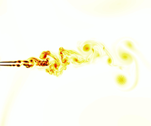



1. Introduction
The flow of a low-viscosity fluid at high speed is chaotic in nature. The energy injected to sustain this state is transferred from large to small eddies, down to a particular scale from which it is dissipated by the viscosity of the fluid (Kolmogorov Reference Kolmogorov1941). Conventional turbulence in three dimensions fulfils this description, whereas new phenomena appear in two dimensions. Energy transfer in two-dimensional (2-D) turbulence is dictated by a double cascade scenario: an inverse cascade of kinetic energy to large scales, and a direct cascade of enstrophy (squared vorticity) to small scales (Kraichnan Reference Kraichnan1967; Batchelor Reference Batchelor1969; Boffetta Reference Boffetta2007). Certainly, no physical system is 2-D in reality, though 2-D turbulence becomes relevant if one spatial direction is greatly constrained, e.g. by geometry (Boffetta et al. Reference Boffetta, De Lillo, Mazzino and Musacchio2012; Boffetta & Ecke Reference Boffetta and Ecke2012). For instance, the large-scale motions in atmospheric flows comply with 2-D turbulence (Charney Reference Charney1971; Nastrom, Gage & Jasperson Reference Nastrom, Gage and Jasperson1984; Lindborg Reference Lindborg1999). In this case, the flow domain is subdued to a large aspect ratio: the horizontal lengths are much larger than the height of the atmospheric layer.
The confinement in thin layers can induce a rich phenomenology in turbulent flows that, if forced at intermediate scales, produces a split energy cascade (Smith, Chasnov & Waleffe Reference Smith, Chasnov and Waleffe1996; Celani, Musacchio & Vincenzi Reference Celani, Musacchio and Vincenzi2010; Alexakis & Biferale Reference Alexakis and Biferale2018). Under these circumstances, a portion of the energy flows to the large scales in a 2-D fashion. Conversely, the remaining part cascades toward the small viscous scales. Interestingly, a direct cascade of enstrophy can develop simultaneously at scales smaller than the forcing but larger than the thickness of the layer, and three-dimensionality becomes relevant only at much smaller scales (Musacchio & Boffetta Reference Musacchio and Boffetta2017). Nevertheless, the presence of physical confinement (e.g. using solid boundaries) is not compulsory to observe the split energy cascade. In fact, numerical simulations in a fully periodic box with one dimension much smaller than the others have shown this phenomenon (Smith et al. Reference Smith, Chasnov and Waleffe1996; Celani et al. Reference Celani, Musacchio and Vincenzi2010). Despite this, its occurrence changes with the boundary conditions. For example, the development of the shear layer in wall-bounded flows restricts the development of 2-D dynamics (Byrne, Xia & Shats Reference Byrne, Xia and Shats2011; Boffetta et al. Reference Boffetta, Musacchio, Mazzino and Rosti2023).
Here, we consider a planar jet, i.e. the flow is injected through a plane slit of half-width  $h$ in a computational box periodic in the vertical direction
 $z$. We adopt a shear-thinning fluid in which the viscosity decreases nonlinearly for increasing values of the shear rate. A similar flow configuration, although at a much higher characteristic Reynolds number, can be found at the outflow of a river into the sea. Differences in salinity, temperature and density between the freshwater stream and the salt water can impede mixing, thus leading to the formation of a stratified flow with a (thin) layer of freshwater flowing over salt water. The presence of suspended bacteria and microalgae in the freshwater stream grants non-Newtonian features to the fluid, such as shear-dependent viscosity (Al-Asheh et al. Reference Al-Asheh, Abu-Jdayil, Abunasser and Barakat2002; Zhang et al. Reference Zhang, Jiang, Chen, Chou, Yan, Zuo and Zhang2013). Our simulations are performed at a much lower value of the Reynolds number, hence there is no direct application of our findings to the flowing regimes found at the outflow of a river; the low value of the Reynolds number allows instead for direct comparisons with experiments. The present configuration can be achieved easily in laboratory experiments; the shear rheology of the fluid used in our simulations corresponds to that of a 100:60 mM CPyCl:NaSal worm-like micelle solution (Haward, Hopkins & Shen Reference Haward, Hopkins and Shen2021). This work thus constitutes a preliminary step in understanding the flow dynamics of geophysical flows, such as the outflow of a river rich in bacteria or microalgae, which are instead characterized by a much larger Reynolds number. The selected parameters make our numerical set-up easily testable by experiments (recent experimental work by Yamani et al. (Reference Yamani, Raj, Zaki, McKinley and Bischofberger2023) addressed the flow of a viscoelastic planar jet at low Reynolds number), whereas the effect of physical confinement is attenuated by the shear-thinning characteristic of the fluid, which reduces the extent of the shear layer (viscosity decreases at the wall boundaries in the experimental set-up).
Within this framework, we show that when the thickness of the domain is large, the flow is completely three-dimensional (3-D), while when it is small, it is fully 2-D. Interestingly, for intermediate cases, the flow spatially transitions from 3-D close to the inlet to 2-D further downstream, with the two regimes being connected by a region of mixed-dimensional turbulent dynamics where the constraint modulates the largest scales towards two dimensions, and the smaller ones remain 3-D. We indeed observe, at intermediate levels of vertical constraint, a multi-cascade process, where both a direct cascade of energy at small scales and a direct cascade of enstrophy at large scales coexist.
2. Numerical method
The motion of the incompressible, shear-thinning fluid is governed by the mass and momentum conservation equations,
 $$\begin{gather} \boldsymbol{\nabla}\boldsymbol{\cdot} \boldsymbol{u} = 0, \end{gather}$$
 $$\begin{gather}\rho \left(\frac{\partial \boldsymbol{u}}{\partial t} + \boldsymbol{u}\boldsymbol{\cdot}\boldsymbol{\nabla}{\boldsymbol{u}}\right) ={-}\boldsymbol{\nabla} p + \boldsymbol{\nabla}\boldsymbol{\cdot} [\mu(\dot\gamma)\, (\boldsymbol{\nabla}\boldsymbol{u}+\boldsymbol{\nabla}\boldsymbol{u}^{\rm T})], \end{gather}$$
respectively. In the above equations,  $\boldsymbol {u}$ is the local flow velocity,
 $\rho$ is the density,
 $p$ is the pressure, and
 $\mu$ is the local viscosity. We adopt an inelastic, shear-thinning fluid, whose behaviour is defined via the Carreau fluid model (Bird, Hassager & Abdel-Khalik Reference Bird, Hassager and Abdel-Khalik1974). The local viscosity
 $\mu$ depends on the local shear rate
 $\dot \gamma$ as
 \begin{equation} \mu(\dot\gamma) = \mu_{\infty} + (\mu_0 - \mu_{\infty}) [1 + (\lambda \dot{\gamma})^{2}]^{{(n-1)}/{2}},\end{equation}
where  $\lambda$ is the fluid consistency index, and
 $\mu _0$ and
 $\mu _{\infty }$ are the zero-shear viscosity and the viscosity for
 $\dot {\gamma } \rightarrow \infty$, respectively. We set the power-law index
 $n = 0.2$, thereby obtaining a strong shear-thinning effect. The local shear rate is defined as
 $\dot \gamma =\sqrt {2\boldsymbol{\mathsf{S}}:\boldsymbol{\mathsf{S}}}$, where
 $\boldsymbol{\mathsf{S}}=(\boldsymbol {\nabla }\boldsymbol {u}+\boldsymbol {\nabla }\boldsymbol {u}^{\rm T})/2$ is the shear rate tensor.
The Navier–Stokes equations are discretized on a uniform, staggered, Cartesian grid; the fluid velocities are located at the cell faces, whereas pressure and viscosity are defined at the cell centres. The fluid viscosity is updated at every time step following (2.3). The spatial derivatives are approximated using second-order finite differences in all directions. The system is advanced in time through a second-order Adams–Bashforth scheme coupled with a fractional step method (Kim & Moin Reference Kim and Moin1985). The divergence-free velocity field is enforced by solving the Poisson equation for the pressure using an efficient solver based on the fast Fourier transform. We resort to the domain decomposition library 2decomp (http://www.2decomp.org) and the MPI protocol to parallelize the solver. The numerical solver is implemented in the in-house solver Fujin (https://groups.oist.jp/cffu/code).
3. Problem set-up
We have addressed this study by means of 3-D direct numerical simulations; the computational box has sizes  $L_x=160h$ in the streamwise direction,
 $L_y=240h$ in the jet-normal direction, and
 $0.83h \le L_z \le 13.33h$ in the spanwise direction. The vertical length
 $L_z$ is varied among simulations: we consider five distinct simulations with
 $L_z = 0.83h, 1.67h, 3.33h, 6.67h, 13.33h$, respectively. The thinnest domain (
 $L_z = 0.83h$) introduces a strong vertical constraint in order to allow the development of a 2-D flow, which is progressively relaxed as
 $L_z$ is increased, while still maintaining a thin computational domain, so
 $L_z \ll L_x \sim L_y$. The planar jet is generated by fluid injected with a uniform velocity
 $U$ through a planar slit of width
 $2h$ spanning the entire height of the domain (
 $z$ direction). At the inlet boundary, we impose no-slip and no-penetration boundary conditions, with an exception made for the inlet portion, where we impose a plug-flow velocity profile. At the outlet boundary (
 $x = L_x$), we use a non-reflective boundary condition (Orlanski Reference Orlanski1976). At the side boundaries (
 $\kern0.09em y = 0$ and
 $y = L_y$), we impose free-slip and no-penetration boundary conditions. Finally, at the top and bottom boundaries (
 $z = 0$ and
 $z = L_z$), we impose periodic boundary conditions.
We select a low value of the inlet Reynolds number (ratio of inertial to viscous effects)  $Re = \rho h U / \mu _{0} = 20$. It should be noted that Newtonian planar jets are laminar at this value of
 $Re$ (Sato & Sakao Reference Sato and Sakao1964; Sureshkumar & Beris Reference Sureshkumar and Beris1995; Deo, Mi & Nathan Reference Deo, Mi and Nathan2008; Soligo & Rosti Reference Soligo and Rosti2023), thus any turbulent motion is caused exclusively by the shear-thinning in the flow. Turbulence, however, is still Newtonian, as it originates by the prevalence of inertial over viscous terms. The non-Newtonian character of the flow indeed promotes the onset of the instability, so the transition to turbulence is at markedly lower
 $Re$ compared with Newtonian planar jets (Ray & Zaki Reference Ray and Zaki2015; Soligo & Rosti Reference Soligo and Rosti2023; Yamani et al. Reference Yamani, Raj, Zaki, McKinley and Bischofberger2023). The non-Newtonian contribution is described using the Carreau number, defined as
 $Cu = h \lambda / U = 100$. The ratio between the zero-shear viscosity and the infinite-shear viscosity is set to
 $\mu _0 / \mu _{\infty } = 50$.
To verify the independence of our results on the specific parameters selected, we perform two additional simulations at a set  $L_z=3.33h$, and we double either the Reynolds number (
 $Re = 40$) or the Carreau number (
 $Cu = 200$). The reference case (
 $L_z=3.33h$,
 $Cu=100$ and
 $Re=20$) exhibits a mixed-dimensional turbulent regime, where features from 2-D and 3-D turbulence are found simultaneously in the flow (see figure 1). In the cases at higher
 $Re$ or
 $Cu$, we expect turbulence to be enhanced. The Reynolds number is increased by reducing the zero-shear viscosity (and consequently the infinite-shear viscosity, defined as
 $\mu _{\infty } = \mu _0 /50$), whereas the Carreau number is increased by changing the fluid consistency index
 $\lambda$, keeping the zero-shear and infinite-shear viscosities unchanged. This way, the transition towards the infinite-shear viscosity occurs at a smaller shear rate compared with the case at
 $Cu=100$.
Effect of the constrained dimension  $L_z$ in the turbulent planar jets. (a–c) Magnitude of the instantaneous vorticity field
 $\|\boldsymbol {\omega }\| U^{-1} h$ in the
 $z = L_z/2$ plane for the 3-D, mixed-dimensional and 2-D planar jets, respectively. The insets show a zoomed view of the region near the inlet at
 $x = [ 0, 20h ]$,
 $y = [ -5h, 5h ]$. (d–f) Power spectra of the turbulent kinetic energy computed at the jet centreline at distances
 $x = 40h, 80h, 120h$ from the inlet. The spectra follow the typical
 $f^{-5/3}$ scaling if turbulence is primarily 3-D (red). In 2-D turbulence (blue), instead, the flow exhibits an
 $f^{-3}$ decay that becomes steeper as
 $x$ increases, tending towards
 $f^{-5}$ in the most constrained planar jet.

We adopt a uniform grid spacing in all spatial directions for all cases; in  $x$ and
 $y$, the domain is discretized using
 $N_x \times N_y = 1536 \times 2304$ grid points, while the number of points in the
 $z$ direction depends on the height of the domain, namely
 $N_z = 8, 16, 32, 64, 128$ for increasing heights. We ensured that the grid resolution is adequate by computing the ratio between the grid spacing
 $\varDelta$ and the mean Kolmogorov length scale
 $\eta$:
 \begin{equation} \eta = \left(\frac{\langle \nu \rangle^3}{\langle \varepsilon \rangle} \right)^{1/4}, \end{equation}
where  $\nu$ is the local kinematic viscosity, and
 $\varepsilon$ is the viscous dissipation; angle brackets indicate averaging in time and in the vertical direction
 $z$. In the cases characterized by the highest turbulence intensity,
 $Re=40$ and
 $Cu=200$, the Kolmogorov length scale is always
 $\eta \gtrsim 0.5 \varDelta$ (where
 $\varDelta$ is the grid spacing, uniform in the three directions). The smallest values of the Kolmogorov length scale are encountered at the jet centreline within the region
 $15h < x < 30h$; beyond
 $x = 40h$, the Kolmogorov length scale is always larger than the grid spacing, thus ensuring that the grid resolution chosen is adequate for all cases.
4. Results
4.1. Effect of vertical confinement
Figure 1 shows the impact of  $L_z$ on the turbulent planar jets, in which, as anticipated, the constraint dictates the turbulent regime in the flow. Consequently, the morphology of the vorticity structures changes significantly with
 $L_z$ (see figures 1a–c). We first observe that turbulence is 3-D if the flow is not constrained, i.e. for sufficiently large values of
 $L_z$. A complete different flow structure is instead observed at low values of
 $L_z$, in which large vortices form dipoles (pairs of counter-rotating vortices) that are advected downstream, and no small-scale flow structures are observed, thus indicating that turbulence is mainly 2-D. The flow does not transition in bulk from 3-D to 2-D when changing
 $L_z$, with the planar jet experiencing an intermediate state where both 3-D and 2-D structures are present in the flow at the same time. This transitional regime, hereafter termed mixed-dimensional (or 2.5-D), is characterized by the simultaneous coexistence in the flow of large-scale 2-D and small-scale 3-D structures.
Next, we inspect the energy spectra in figures 1(d–f). Note that we compute the velocity spectra in time rather than in space by recording velocity data over time from a probe placed on the centreline of the jet, similarly to what is done in experiments. Computing the power spectra in time rather than in the vertical direction allows us to have a wider energy spectrum that is not limited by the height of the domain. The equivalence of time and space spectra has been demonstrated in the past (Namer & Ötügen Reference Namer and Ötügen1988; Soligo & Rosti Reference Soligo and Rosti2023). As is clearly shown in the figures,  $L_z$ influences the energy cascade, which depicts a different behaviour depending on the regime of turbulence. First, the least constrained jet shows the conventional
 $f^{-5/3}$ scaling for 3-D turbulence (Kolmogorov Reference Kolmogorov1941). Consistently, we observe the energy cascade typical of 3-D turbulence: the jet instability gives energy to the flow, and it generates large structures that break down in progressively smaller and smaller eddies. As the vortices move downstream, the characteristic shear rate reduces – hence viscosity increases – and energy is dissipated. We expect to recover the power-law scaling for the 3-D turbulence energy cascade as the turbulent motions are Newtonian: they are generated by the competition of inertial and viscous terms (Soligo & Rosti Reference Soligo and Rosti2023). Eventually, dissipation becomes relevant at every scale, and the cascade is impeded: the scaling
 $f^{-5/3}$ is not present at
 $x = 120h$. On the other hand, the most constrained case exhibits 2-D flow and scaling
 $f^{-3}$. Here, the 3-D cascade is clearly disrupted, and 2-D phenomena become dominant (Kraichnan Reference Kraichnan1967; Batchelor Reference Batchelor1969). The change in the flowing regime observed here is due only to the vertical confinement: we adopt a non-Newtonian fluid model that is characterized by the presence of shear-thinning alone (there are no viscoelastic effects). The spectrum becomes steeper as
 $x$ increases, and it eventually seems to saturate at
 $f^{-5}$. The steepening of the energy spectrum agrees with the appearance of dispersed large-size coherent vortices in the flow (Basdevant et al. Reference Basdevant, Legras, Sadourny and Béland1981; McWilliams Reference McWilliams1984; Benzi et al. Reference Benzi, Paladin, Patarnello, Santangelo and Vulpiani1986; Legras, Santangelo & Benzi Reference Legras, Santangelo and Benzi1988). Note that the change in the vertical constraint also alters the instability in the region close to the inlet: for strong vertical constraint (small
 $L_z$), we observe a flapping motion of the shear layers, whereas puffing motion dominates when the constraint is relaxed (large
 $L_z$). The flapping dynamic is associated with the antisymmetric, sinuous mode that destabilizes the flow more substantially, thus injecting more energy (Mattingly & Criminale Reference Mattingly and Criminale1971), as also observed by the energy spectra close to the inlet, which are shifted upwards in two dimensions compared with the 3-D case. Finally, the mixed-dimensional planar jet exhibits features from both 3-D and 2-D planar jets: the scaling
 $f^{-5/3}$ is found close to the inlet, and it changes towards
 $f^{-3}$ downstream. The spectrum becomes slightly steeper further downstream, consistent with the appearance of the coherent vortices. Similarly to the 2-D jet, the flow is more energetic close to the inlet. Very close to the inlet, the vorticity fluctuations look closely related to those in the 3-D case, implying the existence of puffing events connected to the varicose mode (Sato Reference Sato1960; Mattingly & Criminale Reference Mattingly and Criminale1971). However, flapping motions soon become dominant, and the macroscopic vorticity structures resemble those from the 2-D planar jet, thus indicating the presence of the more energetic sinuous mode.
To better characterize the different natures of the turbulent fluctuations at each scale, we now calculate the longitudinal velocity differences  $\Delta u(r) = ( \boldsymbol {u} ( \boldsymbol {x} + \boldsymbol {r} ) - \boldsymbol {u} ( \boldsymbol {x} ) ) \boldsymbol {\cdot } \boldsymbol {r} / | \boldsymbol {r} |$. Concretely, we introduce the third-order structure function
 $S_3(r) = \langle ( \Delta u )^3 \rangle$, where the angle brackets indicate averaging in time and in space, shown in figure 2 for the different cases analysed. Appendix A reports in detail how the computation of the structure function was performed. A remarkable property of
 $S_3$ is that it denotes whether the flow scales are 2-D or 3-D, depending on its sign (Kolmogorov Reference Kolmogorov1991; Lindborg Reference Lindborg1999), and it can help in understanding the direction of the energy and enstrophy fluxes (Bernard Reference Bernard1999; Cho & Lindborg Reference Cho and Lindborg2001; Cerbus & Chakraborty Reference Cerbus and Chakraborty2017). In the particular case of 2-D turbulence,
 $S_3$ is positive (Lindborg Reference Lindborg1999), whereas it is negative if turbulence is 3-D (Kolmogorov Reference Kolmogorov1991). Indeed, we observe that
 $S_3$ is positive (2-D flow) for the most constrained case (
 $L_z = 0.83h$), whereas it is negative (3-D flow) for the least constrained case (
 $L_z = 6.67h, 13.33h$). Furthermore, the scaling of
 $S_3$ outlines the preferred cascade process, thus indicating the direct cascade of enstrophy in the 2-D case (
 $S_3 \sim r^3$), and the direct cascade of energy in the 3-D counterpart (
 $S_3 \sim -r$). While the scaling
 $S_3 \sim r^3$ is visible for 2-D turbulence, we do not observe a clear
 $S_3 \sim -r$ scaling for all 3-D turbulence cases. We do not find evidence of an inverse mechanism of energy transfer toward the large scales in the 2-D case. This is not surprising if we consider that energy is injected in the flow through the planar slit, thus not forcing the flow at any intermediate scale (Boffetta Reference Boffetta2007; Boffetta & Ecke Reference Boffetta and Ecke2012). More interestingly, turbulence is characterized by a mixed-dimensional regime for the right choice of
 $L_z$. The 2-D and 3-D scales are present simultaneously in the flow for
 $L_z = 1.67h, 3.33h$. In these cases, large scales are 2-D, while the small ones are 3-D, with the transition between regimes happening at some intermediate scale. This transition is strongly dependent on the height of the domain, and it can be delayed further in
 $x$ for increasing values of
 $L_z$.
Third-order structure functions  $S_3$ of the longitudinal velocity fluctuations for different vertical constraints
 $L_z$. We compute
 $S_3$ at
 $x = 40h$ at the flow centreline for each planar jet:
 $L_z = 0.83h, 1.67h, 3.33h, 6.67h, 13.33h$. We show the absolute value
 $| S_3 |$ for clarity, and we indicate with colours whether
 $S_3$ is positive (blue) or negative (red), so that the corresponding turbulent scales are either 2-D or 3-D. Consequently, the scaling for
 $| S_3 |$ changes as
 $L_z$ is shifted towards larger values. We report also the two scalings:
 $S_3 \sim r^3$ if turbulence is 2-D, corresponding to a direct cascade of enstrophy, and
 $S_3 \sim -r$ if it is 3-D, thus denoting a direct cascade of energy. The plots are shifted vertically for better readability.

To further investigate the transition between regimes, we choose a mixed-dimensional planar jet, in particular  $L_z = 3.33h$, and we calculate
 $S_3$ repeatedly at several distances from the inlet. Results are summarized in figure 3(a). Close to the inlet, the flow is 3-D; the effect of the vertical constraint does not hinder the development of the 3-D regime. The largest flow scale is smaller than the geometrical constraint, thus not compromising the energy cascade of the 3-D flow. We report the presence of a single scaling,
 $S_3 \sim -r$, typical of the direct energy cascade. At intermediate distances
 $x = [ 40h, 100h ]$, a mixed-dimensional regime appears: both 2-D and 3-D regimes coexist, with 3-D turbulence characterizing the small scales, and 2-D turbulence characterizing the large scales. Here, the vertical confinement hinders the development of 3-D turbulence at the largest scales, while it has no effect on the 3-D turbulence at the smallest scales. In this case, we have the simultaneous presence of a direct energy cascade (
 $S_3 \sim -r$) at small scales and a direct enstrophy cascade (
 $S_3 \sim r^3$) at large scales. We report in the inset of figure 3(a) the scale at which the structure function changes sign, i.e. the scale where the flow transitions from 3-D to 2-D, so the largest 3-D scale in the flow. We observe that as soon as the jet thickness, which corresponds to the largest
 $r$, reaches the size of the vertical confinement, the largest scales become 2-D. (The jet thickness is defined as the distance from the centreline at which the streamwise velocity equals half of the centreline velocity.) However, some scales between the largest ones and the vertical confinement
 $L_z$ remain 3-D, causing the largest 3-D structures to be anisotropic. Moving downstream, the anisotropy of the largest 3-D structures grows up to a value approximately
 $3L_z$ at
 $x\approx 60h$, after which the flow becomes more and more 2-D. Eventually, we observe that the flow becomes completely 2-D at the farthest distances from the inlet,
 $x \geq 120h$, where the characteristic flow scales are the largest, and the vertical confinement impedes the development of 3-D flow at all scales. We indeed observe a scaling of
 $S_3$ compatible with the direct enstrophy cascade (
 $S_3 \sim r^3$). The range of scales observed at each distance from the inlet depends on two factors: the characteristic length scale of the jet (the jet thickness) and the local viscosity. Both of these quantities increase with increasing distance from the inlet of the jet; the jet thickness determines the largest scale in the flow, while the local viscosity is among the factors determining the eventual development of 3-D turbulent motions.
Third-order structure functions  $S_3$ of the longitudinal velocity fluctuations at different distances from the inlet. (a) Plots of
 $S_3$ computed at distances
 $x$ uniformly separated along the jet centreline (
 $x = 20h, 30h, \ldots, 140h$) for the 2.5-D turbulent planar jet with
 $L_z = 3.33h$. We indicate whether the turbulent scales are 2-D or 3-D with colours, similarly to figure 2. The plots are shifted vertically for better readability. The inset shows the scale
 $r$ at which
 $S_3$ changes its sign. Red and blue markers are used for fully 3-D and 2-D structure functions, respectively, with purple markers for those showing both regimes. Note that if
 $S_3$ does not change sign, then we mark either the largest 3-D scale or the smallest 2-D one. Plots of
 $S_3$ for (b) the least constrained (
 $L_z = 13.33h$) or 3-D jet, and (c) the most constrained (
 $L_z = 0.83h$) or 2-D jet, are shown in a fashion similar to that in (a), where we computed
 $S_3$ at three distances
 $x = 40h, 80h, 120h$ at the jet centreline. In these cases,
 $S_3$ has the same sign throughout
 $x$, thus displaying a single scaling at all distances dependent on the dimensionality of the flow.

Finally, we perform the same analysis on the least ( $L_z = 13.33h$) and most (
 $L_z = 0.83$) constrained jets at several locations on the jet centreline,
 $x = 40h, 80h, 120h$ (see figures 3b,c). In these cases,
 $S_3$ has the same sign throughout
 $x$, indicating that turbulence is either 3-D (
 $S_3 < 0$) or 2-D (
 $S_3 > 0$) in the planar jet. For the 3-D planar jet, the structure function approaches the scaling for the direct cascade of energy,
 $S_3 \sim -r$, at intermediate values of the separation distance
 $r$. On the other hand, the scaling for
 $S_3$ in the 2-D planar jet shifts towards
 $S_3 \sim r^3$, indicating instead the presence of the direct cascade of enstrophy. More interestingly, the scaling holds for small separation distances further from the inlet. This is in good agreement with the concept of the enstrophy cascade as a space-filling phenomenon, thus being present at very small scales (Benzi et al. Reference Benzi, Paladin, Patarnello, Santangelo and Vulpiani1986). Additionally,
 $S_3$ follows an anomalous behaviour at large and intermediate
 $r$. As observed in figure 1, large-size coherent vortices emerge far away from the inlet, which interrupt the enstrophy cascade. At these distances, turbulence becomes more intermittent as velocity fluctuations are localized in the vortexes.
4.2. Effects of  $Re$ and $Cu$ in 2.5-D turbulence


In the previous subsection, we observed that constraining the flow in the vertical direction leads to a transition in the turbulent flow, from 3-D turbulence (large  $L_z$), to a mixed 2.5-D state (intermediate
 $L_z$), and finally to 2-D turbulence (low
 $L_z$). We now consider an intermediate case,
 $L_z=3.33h$, characterized by mixed-dimensional (2.5-D) turbulence, and investigate the sensitivity of the flow dimensionality on the problem parameters. We separately test the effect of a flow parameter, the inlet Reynolds number
 $Re$, and of the fluid rheology. Specifically, we consider a case at a higher Reynolds number,
 $Re=40$, and a case at a higher Carreau number,
 $Cu=200$. An increase in either parameter results in a higher local Reynolds number. The increase in the inlet Reynolds number is attained by halving the reference, zero-shear viscosity
 $\mu _0$ (the infinite-shear viscosity is reduced accordingly,
 $\mu _\infty =\mu _0/50$), whereas the Carreau number is increased by doubling the fluid consistency index
 $\lambda$ with all other parameters left unchanged. The effect of the power-law index
 $n$ was not tested, as a reduction of
 $n$ leads to negligible changes in the fluid rheology, and an increase of
 $n$ leads to a laminarization of the jet fluid, due to an increase in the local viscosity. An increase in the Carreau number shifts the transition towards the infinite-shear viscosity at lower values of the local shear rate
 $\dot {\gamma }$.
We report data from these two additional cases, for  $Re=40$ (figures 4a,c) and
 $Cu=200$ (figures 4b,d). The turbulent kinetic energy power spectrum (figures 4a,b) shows similar results to the reference case (
 $L_z=3.33h$,
 $Re=20$ and
 $Cu=100$): 3-D and 2-D regimes coexist (large 2-D scales and small 3-D scales). Near the inlet,
 $x=40h$, we observe 3-D turbulence characterized by the
 $f^{-5/3}$ scaling of the energy spectrum; as we move downstream, the vertical constraint forces turbulence to the 2-D regime, as indicated by the scaling
 $f^{-3}$. However, for the case at larger Carreau number,
 $Cu=200$, we observe a steepening of the power spectrum away from the inlet: at
 $x=120h$, the power spectrum approaches the scaling
 $f^{-5}$, similarly to what is observed in the more constrained cases. The cases at higher
 $Re$ or
 $Cu$ are characterized by a widening of the region where the power-law scalings are observed: the wider separation of scales is due to the higher value of the local Reynolds number. Also, the third-order structure functions
 $S_3$, reported in figures 4(c,d) at three different streamwise positions, show that the flow is characterized by a mixed-dimensional regime, similarly to what is observed for the reference case, figure 3(a). We observe that for the
 $Cu=200$ case, the onset of the mixed-dimensional regime occurs at a larger distance from the inlet: at
 $x=40h$, the structure function is negative at each scale, thus denoting the absence of 2-D turbulence. At positions further downstream, both the
 $Re=40$ and
 $Cu=200$ cases show a transition between 2-D and 3-D very similar to the reference case.
Effects of  $Re$ and
 $Cu$ in the mixed-dimensional turbulent planar jet (
 $L_z = 3.33h$). (a,b) The power spectrum computed at the jet centreline at distances
 $x = 40h, 80h, 120h$ from the inlet. The 3-D turbulence scaling
 $f^{-5/3}$ (red) and the 2-D turbulence scaling
 $f^{-3}$ (blue) are reported for reference. (c,d) The third-order structure function
 $S_3$ at increasing streamwise distances,
 $x = 40h, 80h, 120h$. Red markers identify 3-D turbulence, and blue markers identify 2-D turbulence. The expected scalings
 $r$ (3-D) and
 $r^3$ (2-D) are reported for reference. (e) The transition scale
 $r$ at which
 $S_3$ changes sign as a function of the streamwise position. Markers identify the different cases: squares for
 $Re=40$, diamonds for
 $Cu=200$, and circles for the reference case (
 $Re=20$,
 $Cu=100$). The colour of the marker defines the dimensionality of the flow: red for 3-D (
 $S_3<0$), blue for 2-D (
 $S_3>0$), and purple for 2.5-D (
 $S_3$ changes sign). The inset reports the transition scale
 $r$ normalized by the local jet thickness
 $2\delta$.

The scale at which we observe transition between 2-D and 3-D turbulence is reported in figure 4(e) for different streamwise positions. This transition scale is defined as the scale  $r$ where the third-order structure function changes sign, from
 $S_3<0$ (3-D) to
 $S_3>0$ (2-D), and corresponds to the largest 3-D scale attained at the specific streamwise position. We use markers to differentiate the various cases (squares for
 $Re=40$, diamonds for
 $Cu=200$, and circles for the reference case) and colours to identify the regime: red for 3-D turbulence (
 $r$ corresponds to the largest scale,
 $2\delta$), purple for 2.5-D (
 $r$ corresponds to the transition scale), and blue for 2-D (
 $r$ corresponds to the smallest scale considered). As seen in figure 4(d), the case at higher
 $Cu$ shows a later transition, at
 $x > 60h$, whereas the case at higher
 $Re$ exhibits a transition length scale very similar to the reference case. The transition from 3-D to 2.5-D turbulence is initiated at a scale similar to twice the jet thickness,
 $r\approx 1.5\delta$, as shown in the inset in figure 4(e), and as we move downstream, it becomes much smaller than the jet thickness. For the reference and
 $Re=40$ cases, we observe a non-monotonic trend in the transition scale
 $r$ (purple markers), initially increasing up to
 $x=60h$ and decreasing past this streamwise position. The decreasing pattern for
 $x\geq 70h$ is shown as well by the
 $Cu=200$ case, which instead shows only the monotonically decreasing trend (for
 $x\geq 70h$, the first streamwise position at which mixed-dimensional turbulence is reported). The maximum transition scale, achieved at approximately
 $x=70h$, is approximately
 $3L_z$ for all cases. We report as well a difference in the transition from 2.5-D to 2-D among the three cases: the flow becomes 2-D for both the
 $Cu=200$ case (at
 $x=140h$) and the reference case (at
 $x=130h$). The
 $Re=40$ case remains instead characterized by mixed-dimensional turbulence and does not show a transition to 2-D turbulence within the length of the simulation domain. Nevertheless, we observe that the size of the transition scale
 $r$ decays with the streamwise position, thus indicating that eventually the flow will become 2-D at a large enough distance from the inlet. We attribute the difference in the 2.5-D to 2-D transition to the lower viscosity of the fluid: the
 $Re=40$ case is characterized by a lower reference zero-shear (and also infinite-shear) viscosity, thus delaying the transition to 2-D turbulence.
5. Conclusions
We have studied via direct numerical simulations how the vertical confinement of a turbulent planar jet can alter its dimensionality. We show that under the right constraint, a mixed-dimensional (2.5-D) turbulent regime appears, that is characterized by the simultaneous presence of large-size 2-D and small-size 3-D scales. The onset of this particular regime is dictated by the size of the constrained dimension  $L_z$: as soon as the flow scales become larger than
 $L_z$, 2-D flow structures appear. This transition is postponed further downstream as the flow is less constrained (increasing
 $L_z$). Therefore, for sufficiently large
 $L_z$, turbulent scales are simply 3-D along the jet, and the direct cascade of energy is enabled. Conversely, a strong confinement (small
 $L_z$) makes the flow 2-D: the direct cascade of energy is disrupted, and the direct cascade of enstrophy takes place. Both cascades are conserved wherever the mixed-dimensional turbulent state is present: the direct cascade of energy is active at small scales, whereas the direct cascade of enstrophy dominates at large scales. The generality of these findings has been tested: two additional cases, one at a higher inlet Reynolds number and one at a higher Carreau number, have been investigated for the mixed-dimensional case,
 $L_z=3.33$. We report that the mixed-dimensional turbulent regime is still observed at both higher
 $Re$ and higher
 $Cu$: the flow is still characterized by large 2-D and small 3-D scales. The largest transition scale, marking the largest 3-D turbulent scales, is attained at
 $x=70h$ for the three cases (
 $Re=40$,
 $Cu=200$ and reference case). Minor differences are observed in the transition from 3-D to 2.5-D, with the
 $Cu=200$ case showing 2.5-D turbulence further downstream, and in the transition from 2.5-D to 2-D, which does not occur within the computational domain for the
 $Re=40$ case. We expect that considering a turbulent Newtonian jet (at a comparable inlet local Reynolds number) would have similar effects of increasing the inlet Reynolds number (
 $Re=40$ case, see figure 4e): the region characterized by 2.5-D turbulence widens, and the transition to 2-D flow shifts downstream. A Newtonian fluid lacks any shear-thinning properties, so it is not characterized by a local viscosity increasing with the streamwise position, thus allowing smaller turbulent structures to exist over a longer distance from the inlet. To better quantify this effect, a complete comparison with Newtonian turbulence is required, and may be the object of a future study. In addition, when increasing either the Reynolds number or the Carreau number, we found that the mixed-dimensional configuration is an overall more energetic state, thus partially retaining the three-dimensionality in the flow while deferring the emergence of 2-D strong vortical structures further downstream from the inlet. The direct enstrophy and energy cascades, and the respective scalings that we report here, are the same as for a Newtonian fluid: the Carreau fluid is a non-Newtonian fluid model characterized by shear-thinning alone, which allows us to attain Newtonian turbulence at a relatively low Reynolds number.
Acknowledgements
The research was supported by the Okinawa Institute of Science and Technology Graduate University (OIST) with subsidy funding from the Cabinet Office, Government of Japan. M.E.R. also acknowledges funding from the Japan Society for the Promotion of Science (JSPS), grant 24K17210. The authors acknowledge the computer time provided by the Scientific Computing and Data Analysis section of the Core Facilities at OIST, and the computational resources on SQUID provided by the Cybermedia Center at Osaka University through the HPCI System Research Project (project ID hp230018).
Declaration of interests
The authors report no conflict of interest.
Appendix A. Structure function in planar jets
The  $p$th-order structure function is defined as the
 $p$th moment of velocity differences (Frisch Reference Frisch1995):
 \begin{equation} S_p(r) = \langle (\Delta u)^p \rangle. \end{equation}
Angle brackets indicate averaging in time, in the vertical direction  $z$, and over velocity differences separated by the same distance
 $r=|\boldsymbol {r}|$.
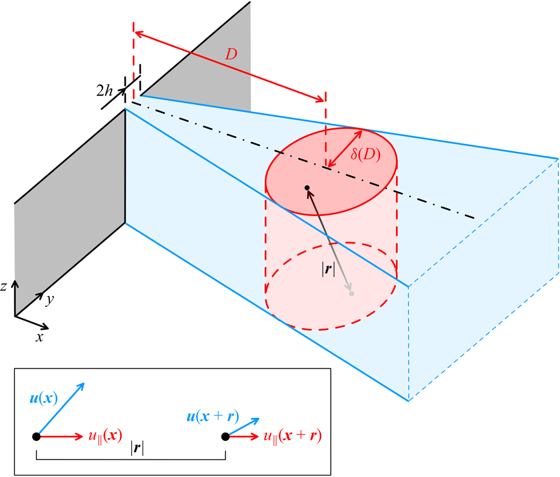
The structure function is computed within a cylinder (in red in the sketch in figure 5) at a set distance  $D$ from the inlet. The cylinder axis is aligned with the vertical direction
 $z$, and its radius is equal to the jet thickness at distance
 $D$ from the inlet, i.e.
 $\delta (D)$. The jet thickness
 $\delta$ is defined as the distance from the centreline at which the streamwise velocity equals half of the centreline velocity. Longitudinal velocity differences
 \begin{equation} \Delta u(r) = u_{||} (\boldsymbol{x} + \boldsymbol{r}) - u_{||} (\boldsymbol{x}) = (\boldsymbol{u} (\boldsymbol{x} + \boldsymbol{r}) - \boldsymbol{u} (\boldsymbol{x}))\boldsymbol{\cdot} \boldsymbol{r} / | \boldsymbol{r}| \end{equation}
are computed across points located at distance  $r$ lying within the cylinder; structure function data are then averaged over time and over a couple of points separated by the same separation distance
 $r$ (angle brackets in (A1)). As the slenderness of the cylinder changes among different vertical constraints and different streamwise positions (for instance, slender cylinder for
 $x=40h$ and
 $L_z=13.33h$, or stocky cylinder for
 $x=120h$ and
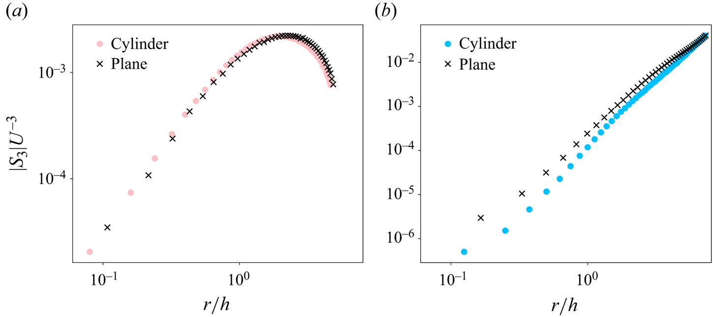
 $L_z=0.83h$), we investigated the effect of different cylinder aspect ratios on the computed structure function. The third-order structure function was thus recomputed considering only a couple of points lying on the same
 $x$–
 $y$ plane, thus eliminating the effect of the separation in the
 $z$ direction. Direct comparison among the structure functions computed within a cylinder and computed on
 $x$–
 $y$ planes showed minimal differences in the values of the third-order structure function, and no difference in its sign (see figure 6).
Calculation of the differences of velocity  $\Delta u$ in the planar jet. The differences of longitudinal velocity
 $u_{||}$ between points separated by a distance
 $r$ are computed among points within the red cylinder.
Third-order structure functions  $S_3$ computed for the cases with (a)
 $L_z = 13.33h$ and (b)
 $L_z = 0.83h$, at a distance
 $x = 40h$ from the inlet. Markers denote whether velocity differences were calculated within a 3-D cylinder (filled circles) or they were limited to
 $x$–
 $y$ planes (black crosses).
The jet thickness  $\delta$ increases with the distance from the inlet
 $D$: as we move away from the inlet, the maximum separation distance
 $2\delta$ increases as well. The maximum separation distance is divided in
 $N_r=60$ uniformly spaced bins; the width of the bins is thus proportional to the jet thickness, and generally increases with the distance from the inlet
 $D$. The smallest width of the bin, found close to the inlet, is about the same size as the grid spacing; as one moves away from the inlet the width of the bin increases, resulting in a limited loss of spatial resolution at the smallest scales (nonetheless smaller than ten grid spacings at the farthest distance considered in the present work). Therefore, in some cases, very small scales may still show 3-D turbulence (and a direct energy cascade); however, they may not be fully detected by the structure function, as they are averaged over the smallest separation distance considered.
In this study, we utilize the third-order structure function  $S_3$, which we show to be a reliable tool to inspect the flow dimensionality and the preferred turbulent cascade process scale by scale. The first derivation of
 $S_3$ resulted in the celebrated Kolmogorov
 $4/5$ law in 3-D turbulence (Kolmogorov Reference Kolmogorov1991):
 $S_3(r) = -\frac {4}{5} \epsilon r$, where
 $\epsilon$ is the mean energy dissipation per unit mass. The
 $S_3$ laws in 2-D turbulence were derived in the late 1990s (Bernard Reference Bernard1999; Lindborg Reference Lindborg1999): for the inverse energy cascade,
 $S_3(r) = \frac {3}{2} P r$ (where
 $P$ is the mean energy injection per unit mass), and for the direct enstrophy cascade,
 $S_3(r) = \frac {1}{8} \zeta r^3$ (where
 $\zeta$ is the mean enstrophy dissipation per unit mass). Cerbus & Chakraborty (Reference Cerbus and Chakraborty2017) related
 $S_3(r)$ to the flux functions:
 \begin{equation} S_3(r) ={-}\frac{3}{2}\,\varPi \left(\frac{a}{r}\right) r + \frac{1}{8}\,Z \left(\frac{a}{r} \right) r^3 + \cdots, \end{equation}
with  $\varPi$ and
 $Z$ being the fluxes of energy and enstrophy, respectively, and
 $a$ being an
 $O(1)$ numerical constant (the quantity
 $a/r$ can be thought of as a wavenumber,
 $k\sim a/r$). Equation (A3) expresses
 $S_3(r)$ as a combination of the energy and enstrophy fluxes, and its sign is affected by values of both fluxes. The previous laws for 2-D turbulence can be derived easily from (A3) (Cerbus & Chakraborty Reference Cerbus and Chakraborty2017).


 Open access

