2 Experimental systems and methods

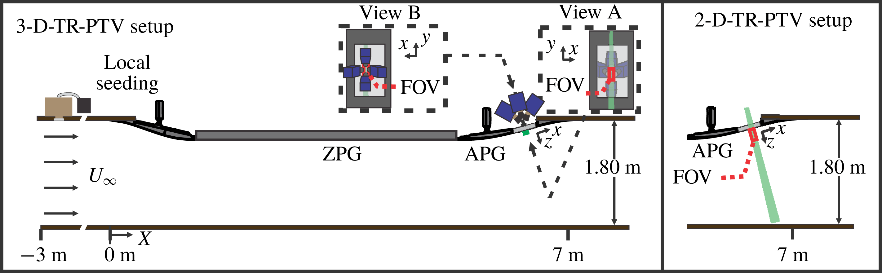
Turbulent boundary layer experiments were performed at the Bundeswehr University Munich in the Atmospheric Wind tunnel Munich (AWM). The Eiffel type wind tunnel has a 22 m long test section with a cross-section of approximately $2~\text{m}\times 2~\text{m}$ . Flow velocities up to $40~\text{m}~\text{s}^{-1}$ can be achieved. A 7 m long polished aluminium boundary layer model consisting of two S-shaped deflections on either end of a 4 m flat plate zero pressure gradient (ZPG) section, was installed along the side wall of the wind tunnel. The adverse pressure gradient (APG) region (downstream of the ZPG part starting at $X=5.75~\text{m}$ and ending at $X=7~\text{m}$ , with an initial boundary layer thickness of 180 mm for $Re_{\unicode[STIX]{x1D70F}}=5000$ ) was fitted with a glass viewing window of size $0.26~\text{m}\times 0.59~\text{m}$ , see figure 1. The $X$ -direction indicates the streamwise distance along the wind tunnel, starting at the beginning of the model. 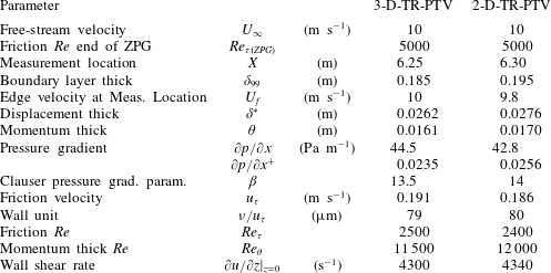The incoming ZPG flow history and global boundary layer parameters at the measurement locations in the APG, such as the edge velocity $U_{f}=0.99U$ , $\unicode[STIX]{x1D6FF}_{99}$ , $\unicode[STIX]{x1D6FF}^{\ast }$ , $\unicode[STIX]{x1D703}$ , $\unicode[STIX]{x2202}p/\unicode[STIX]{x2202}x^{+}$ and $\unicode[STIX]{x1D6FD}$ , were measured in Reuther et al. (Reference Reuther, Scharnowski, Hain, Schanz, Schröder and Kähler2015) for the same boundary layer model and Reynolds number and are reported in table 1.

In order to perform high resolution flow measurements, a local seeding system was installed upstream of the boundary layer wall, providing uniform seeding with a high tracer particle concentration near the wall, see Reuther & Kähler (Reference Reuther and Kähler2018). This local seeding system is located approximately 2 m upstream of the aluminium model. The local seeding system was constructed by covering a $0.05~\text{m}\times 1~\text{m}$ slit in the wind tunnel wall with a large wooden box. On the inside of the tunnel, the slit was covered with an aluminium plate, with a regular arrangement of 2 mm circular holes, mounted flush to the side wall. The wooden box was connected to a conventional impactor seeding generator that creates Di-Ethyl-Hexyl-Sebacat (DEHS) particles with an approximately $1~\unicode[STIX]{x03BC}\text{m}$ mean diameter, (Kähler, Sammler & Kompenhans Reference Kähler, Sammler and Kompenhans2002). The box was filled with tracer particles, which are sucked through the aluminium grid into the boundary layer due to the reduced pressure in wind tunnel. This system is ideal for boundary layer experiments, as the seeding is fed directly into flow region of interest. Furthermore, the location and concentration of the tracer particles can be easily varied by adjusting the position and number of openings in the aluminium plate and the settings of the seeding generator. The disturbance to the flow is minimal as the particles are sucked out of the reservoir by means of the slightly lower pressure in the wind tunnel test section. Moreover, a homogeneous concentration of particles could be reached at the measurement location because of the natural turbulent mixing of the particles inside the boundary layer along the model, as discussed in Reuther & Kähler (Reference Reuther and Kähler2018) in detail.

Figure 1.

Top view of boundary layer model in the Atmospheric Wind Tunnel Munich (AWM) at the Bundeswehr University Munich and the two- and three-dimensional time-resolved particle tracking (2-D- and 3-D-TR-PTV) set-ups.

Table 1.

The global boundary layer parameters, such as the incoming $Re_{\unicode[STIX]{x1D70F}(ZPG)}$ , $\unicode[STIX]{x1D6FF}_{99}$ , $\unicode[STIX]{x1D6FF}^{\ast }$ , $\unicode[STIX]{x1D703}$ and pressure gradient were measured in Reuther et al. (Reference Reuther, Scharnowski, Hain, Schanz, Schröder and Kähler2015). The friction velocity $u_{\unicode[STIX]{x1D70F}}$ and wall shear rate were directly measured in this investigation.

The tracer particles in the APG region were illuminated in a wall-normal plane and a thin wall-parallel volume for the 2-D and 3-D configurations, respectively (see figure 1) by a continuous wave laser (Kvant Laser) with maximum output power of 8 W and $532~\unicode[STIX]{x03BC}\text{m}$ wavelength. For the volumetric measurement, the laser beam was formed into a uniform sheet of 40 mm width and thickness of approximately 1 mm and aligned directly adjacent to the wall. This beam profile was determined by using DataRay Inc. WinCamD-LCM1C beam profiling camera.

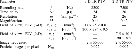
Time-resolved particle image sequences for the planar wall-normal PTV measurements were captured with 1 high-speed CMOS camera with 36 GB of RAM (Dimax-S4, PCO GmbH, LaVision) mounted on top of the wind tunnel to view the laser sheet perpendicularly, see figure 1. Using a 100 mm/f2.8 Makro-Planer Zeiss objective lens with a $2\times$ tele-conversion lens, the resulting resolution in the centre of the field of view (FOV) was ${\sim}26~\unicode[STIX]{x03BC}\text{m}~\text{px}^{-1}$ . By dividing the pixel pitch of the high-speed camera $(11~\unicode[STIX]{x03BC}\text{m}~\text{px}^{-1})$ the resulting magnification in the centre of the FOV was $M=0.42$ , corresponding to a field of view of $7.5~\text{mm}\times 30.3~\text{mm}$ in the streamwise and wall-normal directions, respectively.

The 3-D time-resolved PTV measurements were captured with 4 high-speed CMOS cameras (Dimax-S4, PCO GmbH, LaVision) mounted in a $30^{\circ }$ cross-configuration behind the glass viewing window in the APG, see figure 1. The coordinate system ( $x,y,z$ ) defined in view A corresponds to the streamwise, spanwise and wall-normal directions respectively. Using 50 mm/f2.8 Makro-Planer Zeiss objective lenses and Scheimpflug mounts, the resulting resolution in the centre of the field of view (FOV) was ${\sim}25~\unicode[STIX]{x03BC}\text{m}~\text{pix}^{-1}$ . However, the resolution of the measurement is actually better as the particle images can be located with sub-pixel resolution (Kähler et al. Reference Kähler, Scharnowski and Cierpka2012a ,Reference Kähler, Scharnowski and Cierpka b ). By dividing the pixel pitch of the HS camera the resulting magnification in the centre of the FOV was $M=0.44$ , corresponding to a field of view of $17~\text{mm}\times 25~\text{mm}\times 0.8~\text{mm}$ . The boundary layer thickness, determined from previous large field measurements at the measurement location, was $\unicode[STIX]{x1D6FF}_{99}\approx 190~\text{mm}$ . 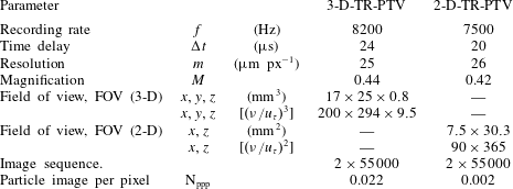An overview of the imaging parameters is given in table 2.

Table 2.

Imaging parameters for particle tracking measurements. The coordinate system ( $x,y,z$ ) corresponds to the streamwise, spanwise and wall-normal directions, respectively.

The evaluation of the data was performed with an in-house tomographic reconstruction method (Fuchs et al. Reference Fuchs, Hain and Kähler2016a , Reference Fuchs, Hain and Kähler2017) and time-resolved particle tracking methods described in Cierpka, Lütke & Kähler (Reference Cierpka, Lütke and Kähler2013a ). For the 2-D imaging, a volume reconstruction was not necessary. Instead the 2-D locations of the particle images were identified using a Gaussian peak detection algorithm and then tracked using the aforementioned time-resolved methods. In contrast to PIV, particle tracking can greatly enhance the spatial resolution as spatial averaging over an interrogation window is avoided (Kähler et al. Reference Kähler, Scharnowski and Cierpka2012a ,Reference Kähler, Scharnowski and Cierpka b ). Since near-wall flows typically feature very strong spatial gradients, especially when small vortices create reverse flow events, particle tracking is also advantageous as no bias errors due to spatial averaging over flow gradients takes place. However, reliable particle identification can be difficult for high seeding concentrations especially when the mean particle distance is much smaller than the mean displacements. Since modern high-speed cameras allow for the time-resolved sampling of the tracer particles, the temporal information was used to enhance the reliability and accuracy of the tracking procedure (Cierpka et al. Reference Cierpka, Lütke and Kähler2013a ; Kähler et al. Reference Kähler, Astarita, Vlachos, Sakakibara, Hain, Discetti, La Foy and Cierpka2016; Schanz et al. Reference Schanz, Gesemann and Schröder2016).

After the particle image tracking, each found trajectory is then unambiguously identified by its common identification number and the algorithm estimates the velocity for each trajectory (particle positions in three dimensions and time) separately. The velocity estimation is based on a second-order polynomial fit of four consecutive positions. Taking the integral of the polynomial curve allows for a correction of the velocity estimation and compensation of bias errors due to curvature effects (Scharnowski & Kähler Reference Scharnowski and Kähler2012). In addition, the vector position is reallocated and placed directly on the polynomial curve instead of in between the two positions as typically done in two-frame representations. This method is especially suited for the correct estimation of the velocity and vector position for trajectories with strong curvature (Cierpka et al. Reference Cierpka, Lütke and Kähler2013a ) as typical for the reverse flow events in the near-wall region of turbulent boundary layers (Bross & Kähler Reference Bross and Kähler2016; Schröder et al. Reference Schröder, Schanz, Geisler and Gesemann2016). However, if only two or three successive positions are known (i.e. end of a trajectory or short trajectories), the velocity estimation is based on the classical first-order displacement estimation and second-order vector positioning (Raffel et al. Reference Raffel, Willert, Scarano, Kähler, Wereley and Kompenhans2018).

3 Trajectory length and validation

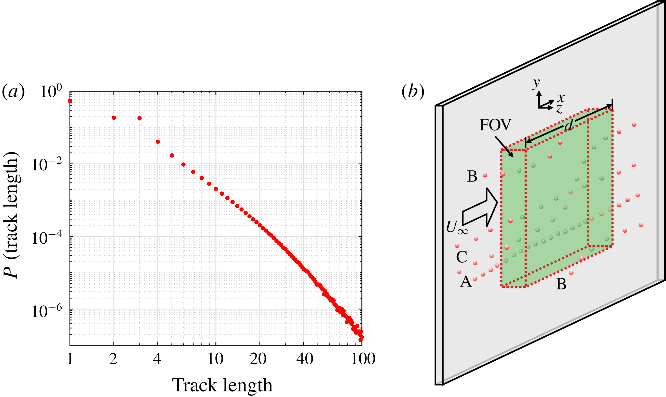
The length of particle trajectories can be quite different depending on the particle velocity and where or when they enter or exit the measurement volume, see figure 2(b). In order to understand the distribution of trajectory lengths, a rectangular measurement volume with a uniform light intensity distribution can be considered, according to figure 2(b). It can be expected that the longest possible continuous tracks, like Track A, appear if a particle enters the volume right at the beginning of the image acquisition and disappear at the end of the volume during the image sequence. If the measurement time is sufficiently long, then the longest tracks are associated with particles that move close to the wall with a low velocity. Therefore, it follows that the faster the particles motion, the shorter the track length will be.

Short trajectories are also likely to appear at the boundaries of the measurement volume when particles locally enter the light volume due to the 3-D flow motion, see particles labelled B. In the present case, the probability of detecting short particle paths at the boundaries is quite large because of the thin extent of the volume in the wall-normal direction and the strong turbulent flow motion close to the wall. Short trajectories can also occur when two independent particle images overlap in the measurement volume due to crossing particle trajectories. This can cause a matching disparity during the volume reconstruction which will break longer tracks into separate tracks of smaller length, as shown by track C. This effect becomes more likely for a relatively dense seeding concentration inside the measurement volume. These points, in combination with spurious or miss-identified particle trajectories, explains the large detection rate of short trajectories, see figure 2(a). Therefore, in order to ensure that only correct trajectories are considered for the analysis, it is reasonable to use the track length as a detection criterion to remove valid but short particle tracks from the flow analysis.

Figure 2.

(a) Trajectory length probability. (b) Ideal laser sheet and trajectories.

Figure 3.

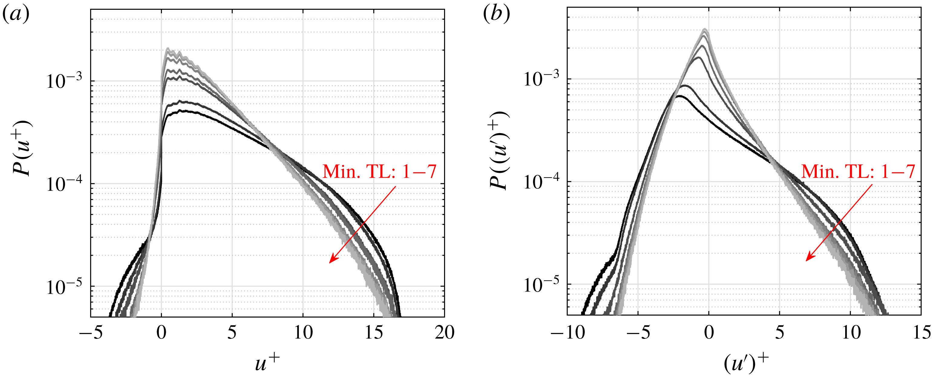
Probability distribution of (a) inner scaled streamwise velocity $u^{+}$ and (b) fluctuations $(u^{\prime })^{+}$ for different minimum track lengths (Min TL) from 1 to 7.

To demonstrate the effect of applying a minimum trajectory length filter, the distributions of instantaneous and fluctuating streamwise velocity for different minimum trajectory lengths between 1 and 7 are plotted in figures 3(a) and 3(b). It is evident from these plots that changing the allowed minimum trajectory length influences the shape of the distribution. The maximum change, particularity in the far right and left tails, occurs between 1 and 3 minimum trajectory lengths. The distribution appears then to converge for minimum trajectory lengths from 4 to 7 for both the instantaneous and fluctuating streamwise velocity in figures 3(a) and 3(b) respectively. Therefore, using a minimum trajectory length of 4 seems appropriate for use in the analysis presented in this paper. Another point to consider from this analysis is how the minimum trajectory length influences the percentage of reverse flow ( $u^{+}<0$ ) detected. In figure 3(a) it appears that more reverse flow events are detected for decreasing minimum trajectory length. However, based on the discussion herein, this is due to outliers that appear as short trajectories. Furthermore, in this investigation a reverse flow event is defined as containing a minimum of two trajectories with $u<0$ (further discussed in § 8). If this criterion is used the probability of reverse flow events with respect to the all detected trajectories remains constant (1.7 %), which means that the detection of reverse flow events in this paper is not influenced by the minimum trajectory length criterion.

4 Mean field

In order to determine the proper inner scaling, the friction velocity, $u_{\unicode[STIX]{x1D70F}}$ , has to be estimated from the slope of the mean velocity profile at the wall. The mean velocity profile was computed by sorting the trajectories into equally spaced bins in the $z$ -direction and extending over the $xy$ -planes. 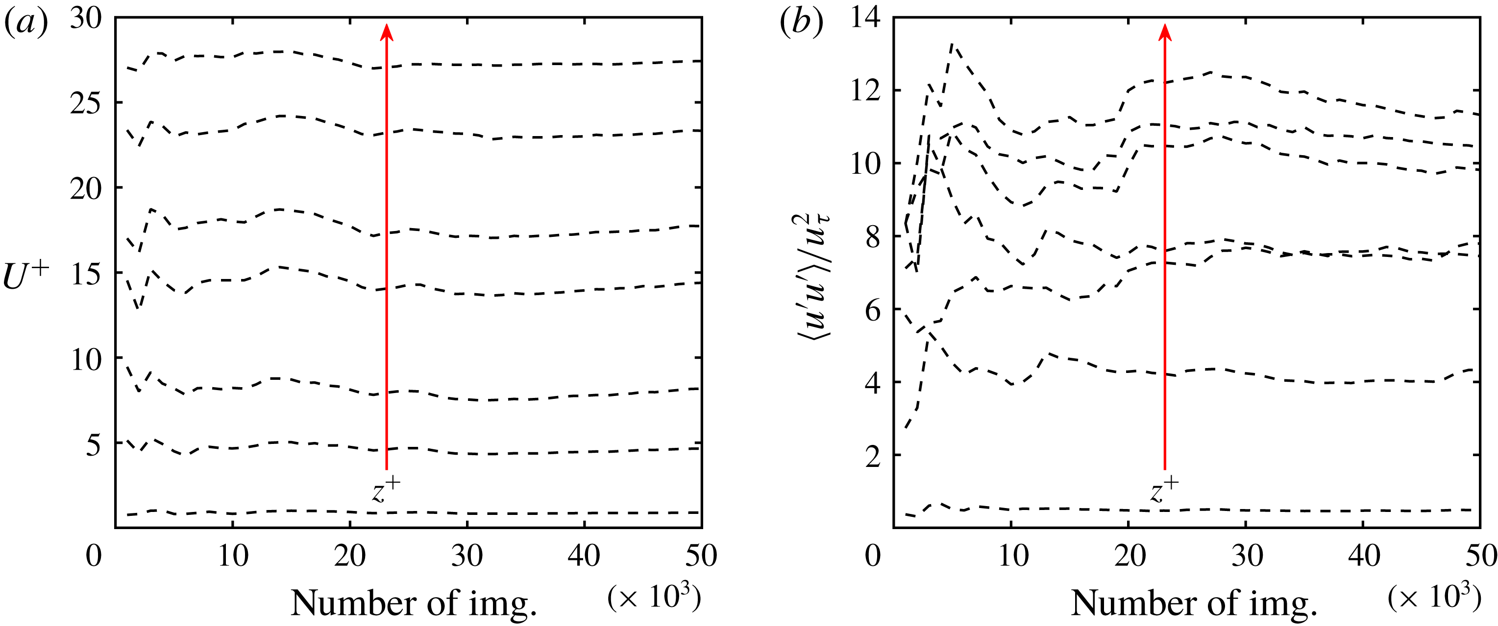For the mean flow results, bins of $z$ -direction spacing $25~\unicode[STIX]{x03BC}\text{m}$ and $12.5~\unicode[STIX]{x03BC}\text{m}$ were used for the 2-D and 3-D measurements, respectively. This bin spacing was selected so that sufficient data points appear within each bin. The number of samples in each bin not only depends on the homogeneity of the tracer particle distribution in the flow but also the number of images used to compute the mean statistics. To demonstrate that sufficient samples were used to calculate the mean statistics, the convergence of the mean streamwise velocity $U^{+}$ and $\langle u^{\prime }u^{\prime }\rangle /u_{\unicode[STIX]{x1D70F}}^{2}$ as functions of the number of sequential image frames used at wall-normal distances $z^{+}=1$ , 5, 10, 50, 100, 200 and 300 are plotted in figures 4(a) and 4(b). These plots demonstrate that the mean streamwise velocity is already well converged for all wall-normal locations at approximately 40 000 images. The fluctuations in figure 4(b) appear to require more than 50 000 samples to completely converge, especially in the log-law region. However, after 40 000 images the variation of the mean velocity fluctuations (figure 4 b) with increasing number of images is less than 2 %.

Figure 4.

(a) Convergence of $U^{+}$ and (b) $\langle u^{\prime }u^{\prime }\rangle /u_{\unicode[STIX]{x1D70F}}^{2}$ as functions of the number of sequential images used at wall-normal distances $z^{+}=1$ , 5, 10, 50, 100, 200 and 300.

The position of the wall is also important for the proper inner scaling and wall shear rate calculations, $\unicode[STIX]{x2202}u/\unicode[STIX]{x2202}z|_{z=0}$ . In the 2-D measurement the orientation of the camera and the light sheet allows for the visualization of both the particle image and its reflection on the glass viewing window. The wall position is then calculated by applying the parallax correction method outlined in Cierpka, Scharnowski & Kähler (Reference Cierpka, Scharnowski and Kähler2013b ) and Fuchs et al. (Reference Fuchs, Bross, Scharnowski and Kähler2018) for each particle–mirror image pair. For the 3-D measurement, the wall position is directly determined from the original camera calibration. For this experimental configuration a dual plane calibration target is placed directly on the window, which results in the $z=0$ location of the reconstructed volume being at the wall position. This calibration procedure is only possible when the wind tunnel is not operating. Therefore, to account for any small shift in the wall position due to the negative pressure difference between the inside and outside of the test section, the wall position can be confirmed in two other ways. First, the distribution of the reconstructed particle images in the $z$ -direction clearly shows any shift in the wall location. Furthermore, a linear fit of the mean streamwise velocity profile will give a $z$ -intercept corresponding to the correct wall position. Comparing the aforementioned methods made it possible to determine, with relative certainty, that the wall shifted a constant 0.05 mm during in all experiments presented herein.

Moreover, at the far edges of the measurement volume, the number of particles imaged will be limited due to the intensity profile of the laser. In these regions, the low number of particle images may have an effect on the statistical quantities due to outliers. Therefore, in all regions outliers are detected and removed and the mean value is calculated from a continuous distribution (Gauss fit) of the particle images in each bin. With this fit applied, the mean field in each bin can be calculated by either taking the peak of the Gauss fit or taking the mean of values within $2\unicode[STIX]{x1D70E}$ . 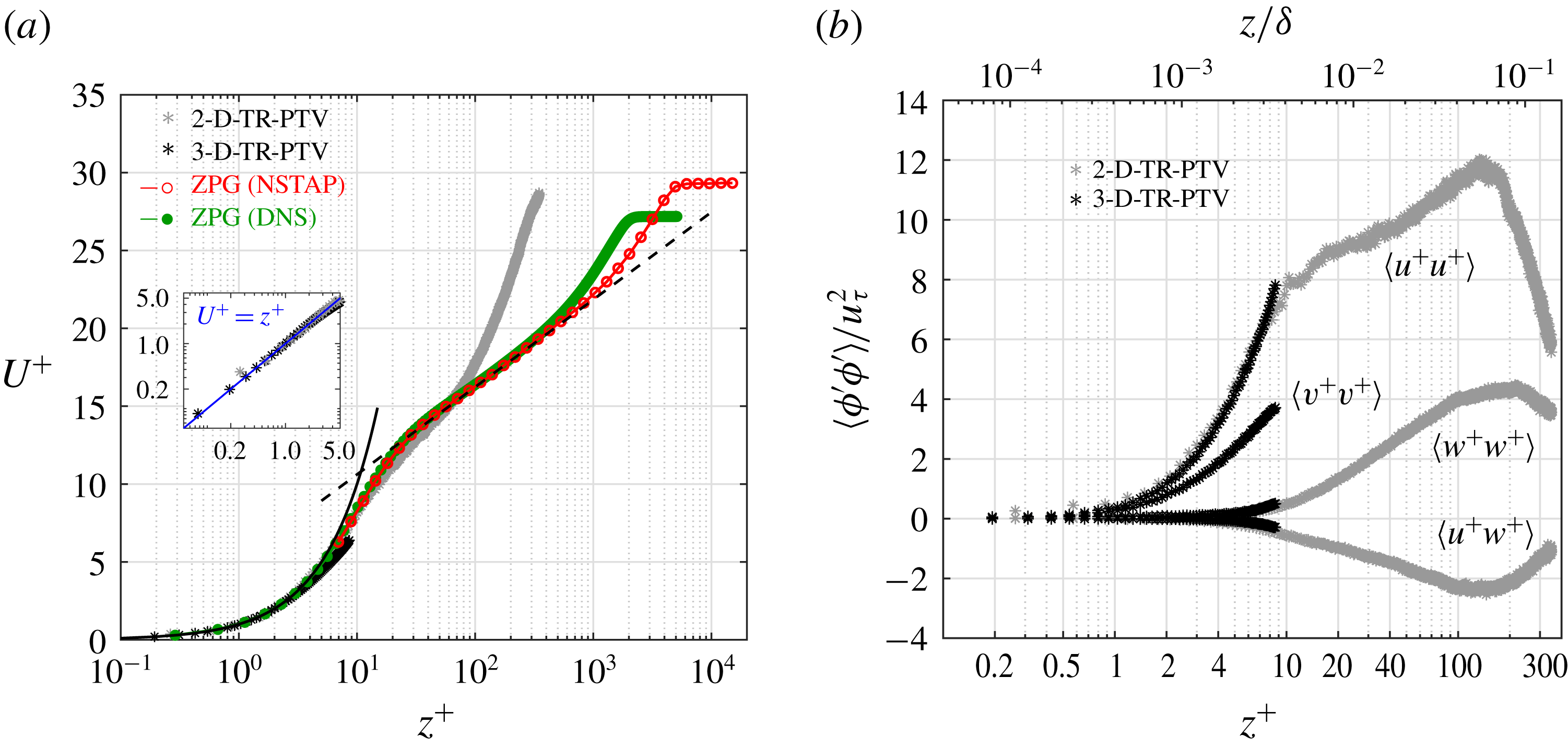For this investigation, velocities within $2\unicode[STIX]{x1D70E}$ of the fit applied to each bin were used to create the mean field and corresponding Reynolds Stress plots shown in figures 5(a) and 5(b), respectively.

Figure 5.

(a) Mean streamwise velocity $U^{+}$ and (b) Reynolds stress profiles versus wall-normal distances in viscous and outer scaling. In addition to the 2-D- and 3-D-TR-PTV data for an APG turbulent boundary layer at $Re_{\unicode[STIX]{x1D70F}}\approx 2500$ ( $Re_{\unicode[STIX]{x1D70F}(ZPG)}=5000$ in the preceding ZPG section) or $Re_{\unicode[STIX]{x1D703}}\approx 12\,000$ and Clauser pressure gradient parameters $\unicode[STIX]{x1D6FD}\approx 14$ , nanoscale thermal anemometry probe (NSTAP) measurements at $Re_{\unicode[STIX]{x1D70F}}=6000$ (Samie et al. Reference Samie, Marusic, Hutchins, Fu, Fan, Hultmark and Smits2018) and DNS computations at $Re_{\unicode[STIX]{x1D70F}}\approx 2000$ or $Re_{\unicode[STIX]{x1D703}}\approx 6500$ (Sillero, Jiménez & Moser Reference Sillero, Jiménez and Moser2013) of a ZPG turbulent boundary layer are plotted in (a). Also shown is the $U^{+}=z^{+}$ indicated by the solid line and the dashed line represents $U^{+}=\log (z^{+})/0.41+5.0$ .

Very good agreement between the 2-D- and 3-D-TR-PTV data sets for both the mean velocity and Reynolds stresses is seen in figures 5(a) and 5(b). Only for $z^{+}>8$ are the 3-D results slightly biased towards smaller velocities. This can be explained by taking into account two effects. First, the large displacements at the edge of the volume reduce the detection probability. In effect the detection of smaller velocities become more likely at the outer edge of the measurement volume. Second, the slightly elongated particle images in this faster moving region increase the reconstruction uncertainty in this region. In the forgoing sections, most of the analysis involving the 3-D data only considers the regions where $z^{+}<8$ .

For this data set it appears that correct mean values were achieved for between $0.1<z^{+}<8$ and $0.2<z^{+}<310$ for the 3-D- and 2-D-TR-PTV data sets respectively. The standard deviation of the mean velocity values was estimated to be no larger than $0.05~\text{m}~\text{s}^{-1}$ . Due to having reliable data points in the linear region ( $U^{+}=z^{+}$ ) of the turbulent boundary layer flow, calculating the viscous scaling is straightforward. A linear fit of $\bar{u}$ versus $\bar{z}$ in the region $1<z^{+}<5$ , where $u=\bar{u}+u^{\prime }$ and $\bar{z}$ is the average bin position in the $z$ -direction, allows for the calculation of $u_{\unicode[STIX]{x1D70F}}=\sqrt{\unicode[STIX]{x1D708}\,\text{d}\bar{u}/\text{d}\bar{z}}|_{z=0}$ and the $z$ -intercept indicates the wall location. Therefore, $U^{+}=\bar{u}/u_{\unicode[STIX]{x1D70F}}$ , $u^{+}=\bar{u}/u_{\unicode[STIX]{x1D70F}}$ and $z^{+}=zu_{\unicode[STIX]{x1D70F}}/\unicode[STIX]{x1D708}$ can directly be calculated. The friction velocity was found to be $u_{\unicode[STIX]{x1D70F}}=0.191~\text{m}~\text{s}^{-1}$ which corresponds to a viscous length of $\unicode[STIX]{x1D708}/u_{\unicode[STIX]{x1D70F}}=79~\unicode[STIX]{x03BC}\text{m}$ for the 3-D data set. Correspondingly, for the 2-D data set, $u_{\unicode[STIX]{x1D70F}}=0.186~\text{m}~\text{s}^{-1}$ and $\unicode[STIX]{x1D708}/u_{\unicode[STIX]{x1D70F}}=80~\unicode[STIX]{x03BC}\text{m}$ . The suitability of the linear fit for the very near-wall region ( $z^{+}<5$ ) is plotted in the zoomed-in inset in figure 5(a). To further corroborate the $u_{\unicode[STIX]{x1D70F}}$ values calculated from this linear fit, a modified composite profile proposed for the inner scaled region proposed in Chauhan, Monkewitz & Hassan (Reference Chauhan, Monkewitz and Hassan2009) was applied to the 2-D-PTV data set for $z^{+}=0.1{-}10$ . The resulting $u_{\unicode[STIX]{x1D70F}}$ from this fit was 0.182, which is in good agreement with the value of 0.186 calculated by using a linear fit for $z^{+}<5$ . In addition, the slight differences in these values for 2-D and 3-D sets can be explained by the slightly different streamwise measurement locations, see table 1. The standard deviation of the velocity and displacement for both data sets was estimated to be (in viscous units) 0.3 and 0.1 respectively.

In order to provide a point of reference for the 2-D- and 3-D-TR-PTV mean velocity and Reynolds stress profiles of an APG turbulent boundary layer at $Re_{\unicode[STIX]{x1D70F}}\approx 2500$ (with $Re_{\unicode[STIX]{x1D70F}(ZPG)}=5000~\text{ZPG}$ history) or $Re_{\unicode[STIX]{x1D703}}\approx ~12\,000$ and Clauser pressure gradient parameter $\unicode[STIX]{x1D6FD}\approx 14$ , NSTAP measurements at $Re_{\unicode[STIX]{x1D70F}}=6000$ (Samie et al. Reference Samie, Marusic, Hutchins, Fu, Fan, Hultmark and Smits2018) and DNS computations at $Re_{\unicode[STIX]{x1D70F}}\approx 2000$ or $Re_{\unicode[STIX]{x1D703}}\approx 6500$ (Sillero et al. Reference Sillero, Jiménez and Moser2013) of a ZPG turbulent boundary layer are plotted in figure 5(a). This comparison shows that the viscous and buffer layers of the strong APG turbulent boundary layer overlay nicely with the ZPG cases when scaled with inner (+) units. However, the length of the log-law region significantly shortens for the APG flow when compared to the ZPG profiles. 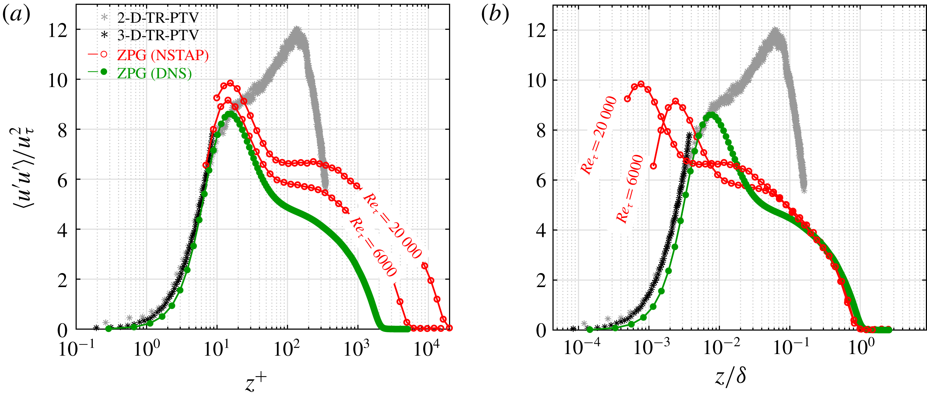Another interesting feature of the strong APG flow is the presence of a large peak in $\langle u^{\prime }u^{\prime }\rangle$ located in the log-law layer or $z/\unicode[STIX]{x1D6FF}\approx 0.065$ in figure 5(b). In ZPG turbulent boundary layers the emergence of a secondary peak/plateau at large Reynolds numbers is widely documented (see § 1) and has been attributed to the presence of energetic superstructures residing in the log-law layer. To compare this observation further, the distribution of $\langle u^{\prime }u^{\prime }\rangle /u_{\unicode[STIX]{x1D70F}}^{2}$ for the strong APG turbulent boundary layer in both inner and outer wall-normal direction scaling in comparison with ZPG profiles from the literature is plotted in figures 6(a) and 6(b). In agreement with the mean streamwise velocity profile, the strong APG streamwise Reynolds stress profiles measured with 2-D- and 3-D-TR-PTV agree well with ZPG DNS results of (Sillero et al. Reference Sillero, Jiménez and Moser2013) in the near-wall region when plotted with $z^{+}$ in figure 6(a). Furthermore, while the prominence of the inner peak for the strong APG is shadowed by the large secondary peak, the location of the inner peak remains rather fixed at $z^{+}\approx 15$ for all the ZPG and APG cases. While the location of the outer peak/plateau moves outward in $z^{+}$ with increasing Reynolds number, the opposite trend occurs when scaling the wall-normal direction with the boundary layer thickness, see figure 6(b). In addition, it can also be observed that while a clearer secondary peak emerges for the highest $Re_{\unicode[STIX]{x1D70F}}$ ZPG case plotted in figure 6(b), the height of the peak is still much lower than the strong APG case at a lower Reynolds number. This suggests that the superstructures associated with the secondary peak in turbulent boundary layers are energized due to the presence of a strong adverse pressure gradient in a similar but more severe way as the effect of increasing the Reynolds number in ZPG turbulent boundary layers (Monty et al. Reference Monty, Harun and Marusic2011; Harun et al. Reference Harun, Monty, Mathis and Marusic2013; Vinuesa et al. Reference Vinuesa, Hosseini, Hanifi, Henningson and Schlatter2017a ). It is also possible that the effect of the strong pressure gradient is to compress the streamwise length of the superstructures which results in a shrinking of the log-law layer observed in figure 5(a) and an increase in the height of the second energetic peak as observed in figures 6(a) and 6(b).

Figure 6.

Mean streamwise Reynolds stress $\langle u^{\prime }u^{\prime }\rangle /u_{\unicode[STIX]{x1D70F}}^{2}$ in (a) viscous and (b) outer wall-normal distance scaling. In addition to the 2-D- or 3-D-TR-PTV data for an APG turbulent boundary layer at $Re_{\unicode[STIX]{x1D70F}}\approx 2500$ ( $Re_{\unicode[STIX]{x1D70F}(ZPG)}=5000$ in the preceding ZPG section) and $Re_{\unicode[STIX]{x1D703}}\approx 12\,000$ and Clauser pressure gradient parameters $\unicode[STIX]{x1D6FD}\approx 14$ , NSTAP measurements at $Re_{\unicode[STIX]{x1D70F}}=6000$ and 20 000 (Samie et al. Reference Samie, Marusic, Hutchins, Fu, Fan, Hultmark and Smits2018) and DNS computations at $Re_{\unicode[STIX]{x1D70F}}\approx 2000$ or $Re_{\unicode[STIX]{x1D703}}\approx 6500$ (Sillero et al. Reference Sillero, Jiménez and Moser2013) of a ZPG turbulent boundary layer.

5 Flow field correlations

In this section the spatio-temporal connection between the flow structures in the viscous sublayer, buffer and log-law regions is examined using multi-point statistics. Using the time information in the recorded data, it is possible to make correlations in both space and time. These types of correlations have played an important role in the statistical analysis of temporal and spatial scales in turbulent flows, see Wallace (Reference Wallace2014) and references therein. In the following section space–time correlations are calculated directly from a 2-D time-resolved data set using the following generalized form,

(5.1) $$\begin{eqnarray}R_{\unicode[STIX]{x1D719}_{i}\unicode[STIX]{x1D719}_{j}}(x_{0},z_{0}+\unicode[STIX]{x0394}z,\unicode[STIX]{x0394}t)=\frac{\langle \unicode[STIX]{x1D719}_{i}(x_{0},z_{0},t_{0})\unicode[STIX]{x1D719}_{j}(x_{0},z_{0}+\unicode[STIX]{x0394}z,t_{0}+\unicode[STIX]{x0394}t)\rangle }{\unicode[STIX]{x1D70E}_{\unicode[STIX]{x1D719}_{i}(x_{0},z_{0},t_{0})}\unicode[STIX]{x1D70E}_{\unicode[STIX]{x1D719}_{j}(x_{0},z_{0}+\unicode[STIX]{x0394}z,t_{0}+\unicode[STIX]{x0394}t)}},\end{eqnarray}$$

where $\unicode[STIX]{x1D719}_{i}$ and $\unicode[STIX]{x1D719}_{j}$ ( $i,j=1,2$ ) are fluctuating velocity or wall shear stress, $\unicode[STIX]{x1D70F}_{W}^{\prime }$ . The location $(x_{0},z_{0})$ is a point at a specific location in the streamwise and wall-normal directions that is then shifted in the wall-normal direction by $\unicode[STIX]{x0394}z$ , and by incremental time steps ( $t_{0}+\unicode[STIX]{x0394}t$ ). In other words the correlation is calculated by selecting a position and time series $(x_{0},z_{0},t_{0})$ and correlating that series for all other wall-normal locations, shifted in time by $\unicode[STIX]{x0394}t$ . In the following correlation plots the vertical and horizontal axes are scaled in both inner and outer normalizations, i.e. $z^{+}=zu_{\unicode[STIX]{x1D70F}}/\unicode[STIX]{x1D708}$ , $z/\unicode[STIX]{x1D6FF}$ , $t^{+}=tu_{\unicode[STIX]{x1D70F}}^{2}/\unicode[STIX]{x1D708}$ and $tU_{f}/\unicode[STIX]{x1D6FF}$ . Furthermore, the correlation calculation is made by averaging sub-samples of the entire record time sequence which are approximately $tU_{f}/\unicode[STIX]{x1D6FF}=300$ or $t^{+}=13\,000$ in length for each time record. The correlations in figures 7(a) and 7(b) are calculated for sub-sets of 1400 images corresponding to $\unicode[STIX]{x0394}t^{+}=\pm 100$ or $\unicode[STIX]{x0394}tU_{f}/\unicode[STIX]{x1D6FF}=\pm 2.32$ . For figure 7(b) the time shift is $\unicode[STIX]{x0394}t^{+}=\pm 25$ or $\unicode[STIX]{x0394}tU_{f}/\unicode[STIX]{x1D6FF}=\pm 0.61$ .

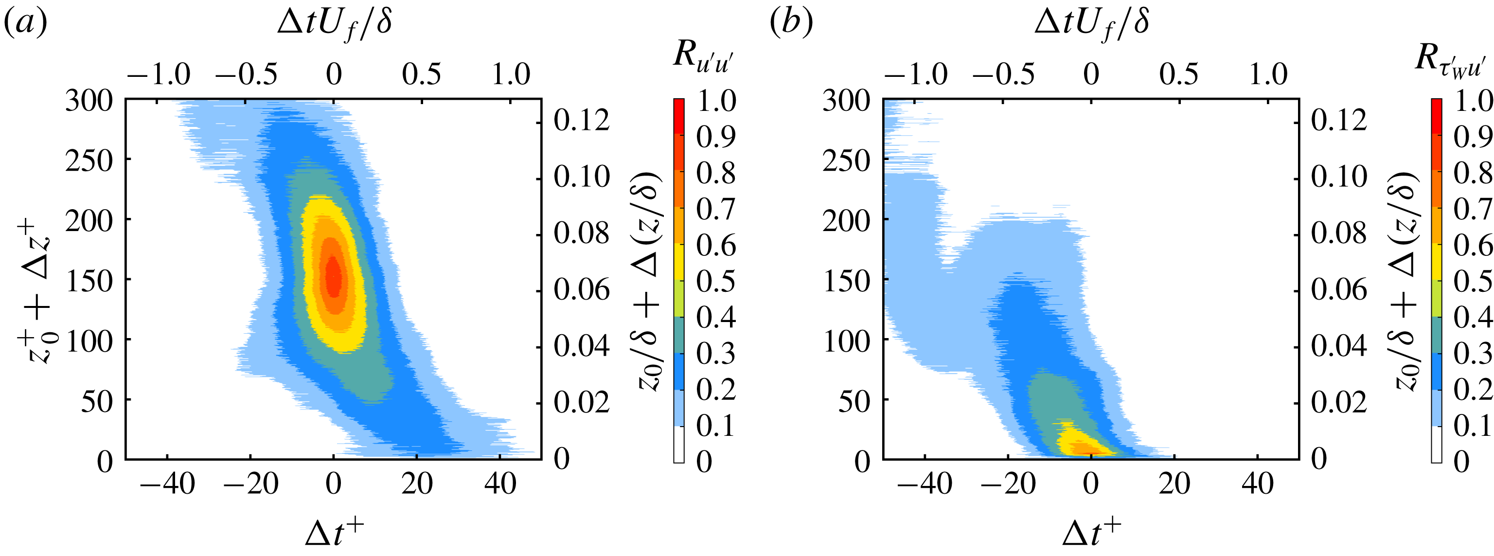
To begin this analysis, the auto-correlation of the streamwise velocity fluctuation $u^{\prime }$ at a starting point near the outer peak ( ${\sim}z_{0}/\unicode[STIX]{x1D6FF}=0.065$ ) is shown in figure 7(a). In this plot a strong positive correlation with almost no time shift within the log-law layer is visible. As the buffer and viscous layers are approached, the correlation shifts in the forward time direction. This phase shift means that it takes some time to detect the correlated flow motion at the wall compared to the location of the reference point. Therefore, this shift indicates forward leaning superstructures similar to the case of a ZPG turbulent boundary layer (Hutchins et al. Reference Hutchins, Monty, Ganapathisubramani, NG and Marusic2011; Buchmann et al. Reference Buchmann, Kücükosman, Ehrenfried and Kähler2016; Baars, Hutchins & Marusic Reference Baars, Hutchins and Marusic2017). More specifically, $R_{u^{\prime }u^{\prime }}$ values between 0.2 and 0.3 persist down to the wall and are positively shifted around $\unicode[STIX]{x0394}t^{+}=25$ or $\unicode[STIX]{x0394}tU_{f}/\unicode[STIX]{x1D6FF}=0.6$ . The correlation level implies that the near-wall field down to the viscous sublayer is strongly modulated by the flow dynamics in the buffer layer and log-law region in accordance with hot-wire measurements (Hutchins & Marusic Reference Hutchins and Marusic2007b ; Mathis et al. Reference Mathis, Hutchins and Marusic2009; Ganapathisubramani et al. Reference Ganapathisubramani, Hutchins, Monty, Chung and Marusic2012). Therefore, it can be concluded without any assumption that the flow motion in the viscous sublayer is modulated by small- and large-scale motions in the buffer and log-law region. The inclination angle of the large-scale motions, which is widely reported for ZPG flows in the range $12^{\circ }{-}16^{\circ }$ Adrian et al. (Reference Adrian, Meinhart and Tomkins2000), Marusic & Heuer (Reference Marusic and Heuer2007), Baars et al. (Reference Baars, Hutchins and Marusic2017), is not trivial for strong APG turbulent boundary layers due to the severely decelerating streamwise convection velocity of superstructures over the strongly curved APG model used in this investigation. However, direct numerical simulations of a self-similar APG turbulent boundary layer reported in Kitsios et al. (Reference Kitsios, Sekimoto, Atkinson, Sillero, Borrell, Gungor, Jiménez and Soria2017) show that the inclination angle of spatial correlations of $R_{u^{\prime }u^{\prime }}$ increases while the streamwise correlation length decreases for increasing APG compared to the ZPG case.

Figure 7.

Space–time correlations (a) $R_{u^{\prime }u^{\prime }}$ , where the starting point is at the outer peak location of the $\langle u^{\prime }u^{\prime }\rangle$ profile ( ${\sim}z_{0}/\unicode[STIX]{x1D6FF}=0.065$ ), and (b) $R_{\unicode[STIX]{x1D70F}_{W}^{\prime }u^{\prime }}$ , where $\unicode[STIX]{x1D70F}_{W}^{\prime }$ is the fluctuating wall shear stress, for an APG turbulent boundary layer at $Re_{\unicode[STIX]{x1D70F}}=2400$ ( $Re_{\unicode[STIX]{x1D70F}(ZPG)}=5000$ in the preceding ZPG section) or $Re_{\unicode[STIX]{x1D703}}=11\,500$ , and Clauser pressure gradient parameter $\unicode[STIX]{x1D6FD}=14$ .

To evaluate the connection of the near and far fields in more detail, $R_{\unicode[STIX]{x1D70F}_{W}^{\prime }u^{\prime }}$ was calculated and plotted in 7(b). As the correlation is positive, the results demonstrate that a high-momentum structure in the buffer layer and log-law region are associated with a positive $\unicode[STIX]{x1D70F}_{W}^{\prime }$ and in turn also show that low-momentum structures are associated with a negative $\unicode[STIX]{x1D70F}_{W}^{\prime }$ at the wall. The shape of the correlation implies that a positive correlation in the wall-normal direction is skewed in the negative time direction. This means that the correlated signal at large wall distances had already passed the $x$ -location when the corresponding signal is measured at the wall. The strong correlation signal above 0.6 between $\unicode[STIX]{x1D70F}_{W}^{\prime }$ and $u^{\prime }$ ends around the buffer layer but similarly to figure 7(a) there is a small correlation value extending into the log-law layer, which indicates the strong relationship between wall shear stress fluctuations and near-wall low-speed streaks. However, there is also a significant correlation between $\unicode[STIX]{x1D70F}_{W}^{\prime }$ and the log-law region which indicates that the turbulent superstructures manipulate $\unicode[STIX]{x1D70F}_{W}^{\prime }$ significantly.

Figure 8.

Space–time correlation $R_{\unicode[STIX]{x1D70F}_{W}^{\prime }w^{\prime }}$ , where $\unicode[STIX]{x1D70F}_{W}^{\prime }$ is the fluctuating wall shear stress and $w^{\prime }$ is the fluctuating wall-normal velocity, for an APG turbulent boundary layer at $Re_{\unicode[STIX]{x1D70F}}=2400$ ( $Re_{\unicode[STIX]{x1D70F}(ZPG)}=5000$ in the preceding ZPG section) or $Re_{\unicode[STIX]{x1D703}}=11\,500$ , and Clauser pressure gradient parameter $\unicode[STIX]{x1D6FD}=14$ .

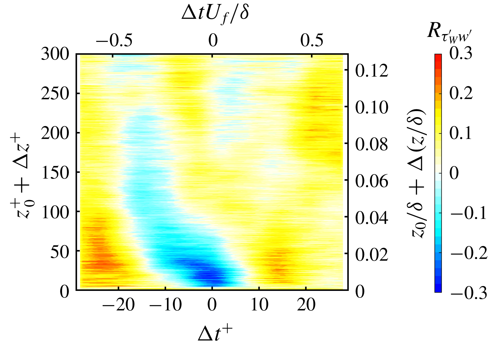
Finally, with the readily available wall-normal velocity fluctuations $w^{\prime }$ , the correlation of the wall shear stress and $w^{\prime }$ can be calculated and is plotted in figure 8. In this plot, a strong positive and negative correlation is visible. This shows that positive wall shear stress $\unicode[STIX]{x1D70F}_{W}^{\prime }>0$ is associated with flow motion towards the wall and negative wall shear stress $\unicode[STIX]{x1D70F}_{W}^{\prime }<0$ is correlated with motion moving away from the wall. This negative correlation of between $-$ 0.1 and $-$ 0.3 with negative time shift extends from the wall to the log layer. The maximum negative correlation appears at ( $-0.85\unicode[STIX]{x0394}t^{+}$ , $17\unicode[STIX]{x0394}z^{+}$ ). In addition, positive correlated regions in the near wall and buffer layer shifted by $\pm 20\unicode[STIX]{x0394}t^{+}$ on either side of the large negative correlated region show a different phase of the relationship between the wall shear stress and the wall-normal velocity. In these regions, negative wall shear stress is associated with flow towards the wall and positive wall shear stress is associated with flow away from the wall. In summary, the results of the direct measurements show that a strong relationship exists between the dynamics of the viscous sublayer and the flow motion in the buffer layer and log-law region.

6 Near-wall uniform-momentum zones

In this section it will be demonstrate that the flow near the wall can be classified into layers of uniform momentum. These regions have been studied and characterized for ZPG turbulent boundary layers in great detail by Meinhart & Adrian (Reference Meinhart and Adrian1995), Adrian et al. (Reference Adrian, Meinhart and Tomkins2000), de Silva et al. (Reference de Silva, Hutchins and Marusic2016), Laskari et al. (Reference Laskari, de Kat, Hearst and Ganapathisubramani2018). However, none of these investigations resolved the near-wall flow features considered in this investigation. In this study, the velocity field in the lower log-law layer, buffer region and viscous sublayer are well resolved and therefore a brief analysis of the UMZs in the near-wall region is done.

Figure 9.

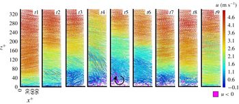
Time trace of trajectories coloured with $u/U_{f}$ for an APG turbulent boundary layer at $Re_{\unicode[STIX]{x1D70F}}=2400$ ( $Re_{\unicode[STIX]{x1D70F}(ZPG)}=5000$ in the preceding ZPG section) or $Re_{\unicode[STIX]{x1D703}}=11\,500$ , and Clauser pressure gradient parameter $\unicode[STIX]{x1D6FD}=14$ . In the top figure a space–time plot is made for $3000t^{+}$ or $70tU_{f}/\unicode[STIX]{x1D6FF}$ , representing 10 500 recorded images. Smaller temporal selections are selected and plotted below the top figure.

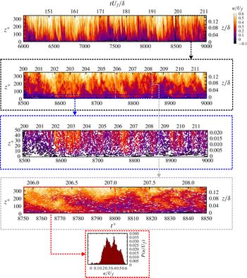
In figure 9 trajectories are coloured with $u/U_{f}$ , where the vertical axis is the wall-normal direction and time is plotted along the horizontal axis. In the top figure a space–time plot is made for $3000t^{+}$ or $70tU_{f}/\unicode[STIX]{x1D6FF}$ , representing 10 500 recorded images. Already in this representation several regions of similar momentum are visible due to the discreet colour bar. Furthermore, it can be seen that the UMZs appear frequently in time and their extent in the wall-normal direction and shape are also clearly visible from the visualization. However, since this view is compressed in the horizontal direction, smaller temporal selections are selected and plotted below the top figure to make the regions more visible. In each successive zoom in, the UMZs in the near-wall region become clearer. From visual inspection it seems that 2–3 UMZs are present in the near-wall region. To make the UMZ analysis more quantitative, a small number of trajectories were selected to create a probability density function (p.d.f.) of the instantaneous velocity, which is plotted in the bottom of figure 9. The p.d.f. was calculated for $50t^{+}$ or $1tU_{f}/\unicode[STIX]{x1D6FF}$ , which is comparable when transformed into space via Taylor’s frozen pattern hypothesis, to previous studies. Selecting a much larger region results in smoothing of the p.d.f. making the individual peaks of the UMZ not visible. In addition, the number of bins used for the histogram was 50, which was doubled and halved with no significant difference in the number of peaks identified. In this particular case, two or possibly three distinct peaks are detected. The peak locations and corresponding UMZ can be seen in the above trajectory plots by visual inspection. A movie showing the evolution of the near-wall UMZs can be found in the supplementary material available at https://doi.org/10.1017/jfm.2019.408 (movie 1).

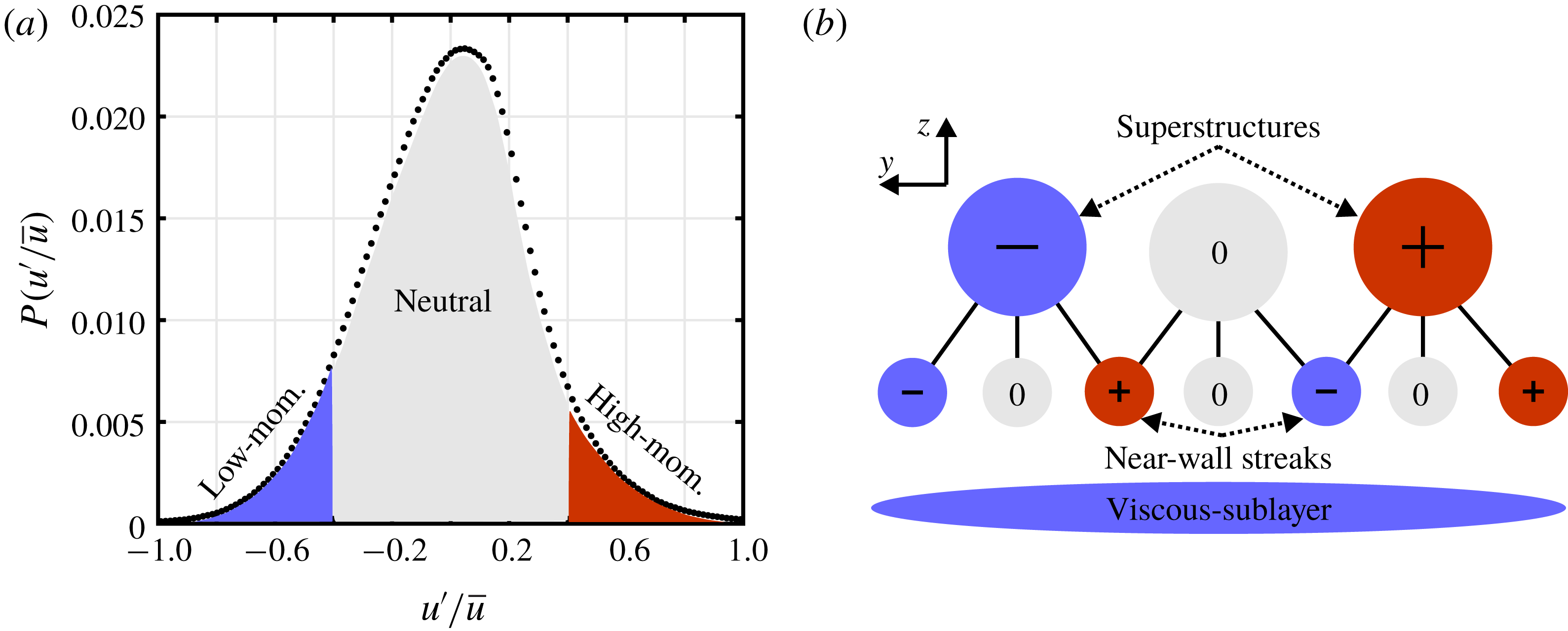
The lowest UMZ is associated with the viscous sublayer, which is visible in the enhanced near-wall view (third from top) in figure 9. The low- and high-speed streaks in the buffer layer form another region of uniform momentum. The third layer is generated by low- and high-momentum superstructures. If we also consider flow regions that convect close to the mean flow velocity (see figure 10 a) we can make a model that illustrates the possible layered UMZ combinations, see figure 10(b). In this model, representative superstructures and near-wall streaks in the buffer layer can be characterized by their streamwise velocity fluctuation magnitude relative to the local mean velocity. In figure 10(b), generalized near-wall streaks and superstructures with either ( $-$ )low- or ( $+$ )high-momentum are shown. In addition, fluid with momentum in between certain thresholds is designated as neutral in figure 10(a) or 0 in figure 10(b). This very general representation is based on the known coherent near-wall streaks and superstructures in the log-law layer. Using this representation of the near-wall and outer region structures, nine different combinations of structures can be made depending on how the superstructures in the log-law region and near-wall streaks and neutral flow are layered. Which means that in addition to the UMZ associated with the viscous sublayer, two additional UMZs with nine possible layering variations are expected based on this model. Therefore, the observation of 2–3 UMZs in figure 9 becomes understandable by taking the viscous sublayer into account. In previous studies, the average number of UMZs detected in ZPG turbulent boundary layers ranged from 3–5 depending on the Reynolds number (de Silva et al. Reference de Silva, Hutchins and Marusic2016). It was also demonstrated that the number of detected UMZs is related to the passage of low- or high-momentum superstructures through the measurement plane and when these superstructures are connected with strong downward or upward motion ( $Q4$ and $Q2$ ) the number of detected UMZs strongly decreases or increases (Laskari et al. Reference Laskari, de Kat, Hearst and Ganapathisubramani2018). In principle these findings show that the momentum of superstructures in the log-law layer and their footprint on the wall are strongly related to the number of instantaneous UMZs. This can also be generally explained by the different possible combinations superstructures layered on near-wall streaks shown in figure 10(b). It is evident that these effects bias the length estimations of superstructures based on spatial correlation calculations towards smaller lengths.

Figure 10.

(a) Probability density function of $u^{\prime }/\bar{u}$ for $z/\unicode[STIX]{x1D6FF}<$ 0.15 with low-, neutral- and high-momentum regions highlighted. (b) Conceptual UMZs based on layering of low-, equal- or high-momentum superstructures and near-wall streaks above the viscous sublayer. The sign indicates the relative magnitude of the absolute velocity.

Figure 11.

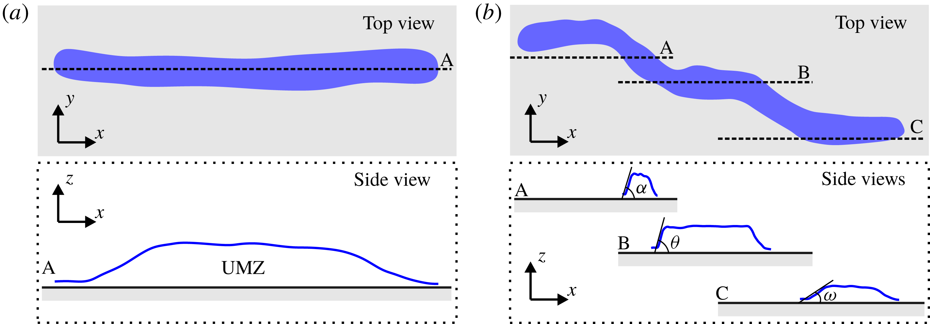
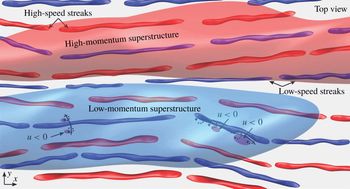
(a) Long streamwise oriented UMZ sliced by measurement plane A. (b) Meandering UMZ sliced by measurement planes A, B and C.

The exact slope of the UMZ depends on how the meandering near-wall streaks are sliced by the measurement plane as indicated in figures 11(a) and 11(b). As the high-speed streaks are wider than the low-speed streaks (Jiménez, Del Álamo & Flores Reference Jiménez, Del Álamo and Flores2004; Lin et al. Reference Lin, Laval, Foucaut and Stanislas2008) they dominate the specific UMZ in the measurement plane. However, when a low-speed streak passes through the measurement domain this is clearly visible. The flow in the log-law region is populated by turbulent superstructures of various lengths, heights and intensities which interact in a complex manner. In addition, the flow structures are faster in this region which makes their extent in the streamwise direction appear shorter. The typical slow layer structure with specific inclination angles becomes visible when a near-wall low-speed streak and a turbulent superstructure are sliced by the measurement plane, as shown in figure 11(a). However, due to the meandering nature of the structure shown in figure 11(b), they are often sliced by the measurement plane at different locations. This leads to variations in length, heights and inclination angles of the UMZ in the side view. If the measurement plane slices through the structure in the middle like the A and B slices (see figure 11 b), the inclination angle of the UMZ will be approximately the same, i.e. $\unicode[STIX]{x1D6FC}\approx \unicode[STIX]{x1D703}$ . However, when the measurement plane slices the structure on the side and not through the middle, see slice C in figure 11(b), the UMZ shown from the side will have a smaller inclination angle $\unicode[STIX]{x1D714}$ and consequently a shorter height than measured in slices A and B. This conceptual diagram illustrates how and when UMZs occur in the measurement plane, in terms of wall-normal and streamwise extents, inclination angle and temporal coherence.

This assessment of the UMZ in this section implies that at least 2–3 UMZs exist in the near-wall region. When considering the flow in the viscous sublayer, streaks in the buffer layer and superstructures in the log-law layer, this analysis is understandable. Therefore, it follows that different regions of uniform momentum form depending on the layering of the coherent structures which is sketched in a general form in figure 10(b). Consequently, the direct interaction between low- and high-speed streaks and superstructures is evident.

7 Space–time visualization

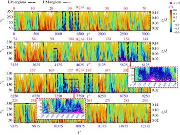
In the previous sections the strong correlation of the flow features in space and time was shown. However, the analysis does not allow for a distinction between low- and high-momentum flow structures. The positive correlation just states that if a velocity fluctuation is positive at a certain location it will be positive in the surrounding area. On the other hand if $u^{\prime }<0$ , the surrounding correlation will also be positive. It is evident from the analysis of Buchmann et al. (Reference Buchmann, Cierpka, Knopp, Schanze, Schröder, Hain and Kähler2014) that the large-scale flow motions can significantly vary in their turbulent kinetic energy and it was also demonstrated that the slope of the correlated flow motion can be quite different depending on which structure is considered for the correlation. Therefore, in order to study how low- and high-momentum large-scale structures alter in time, a space–time plot of the streamwise fluctuation fields over a long time sequence was made, see figure 12.

This plot was made by selecting a thin wall-normal slice of the flow field and plotting all the trajectories passing through that slice with time. In the case of the wall-normal planar data (2-D-TR-PTV), trajectories passing through a thin (streamwise) strip extending from the wall to 350 viscous units over 45 000 image sequences, corresponding to temporal lengths of $t^{+}=12\,500$ or $tU_{f}/\unicode[STIX]{x1D6FF}=293$ , are plotted in figure 12. The trajectories are coloured with the streamwise fluctuating velocity, $u^{\prime }$ , scaled with the local streamwise mean velocity, $\bar{u}$ . A similar approach was used for ZPG turbulent boundary layers in Willert (Reference Willert2015).

The first things immediately visible in figure 12 are the intermittent low- ( $u^{\prime }/\bar{u}<0$ ) and high- ( $u^{\prime }/\bar{u}>0$ ) momentum regions. Since these data are compressed in order to show a long time sequence, these regions in the log layer are actually elongated structures in space. In accordance with the findings in § 5 these regions often go all the way down to the wall, which indicates that a low- or high-momentum structure is aligned with a corresponding low- or high-speed near-wall streak and the dynamics within the viscous sublayer, as already pointed out. Sometimes the regions only exist for $tU_{f}/\unicode[STIX]{x1D6FF}=1{-}2$ and other times there are sustained low- or high-momentum regions that persist for more than $tU_{f}/\unicode[STIX]{x1D6FF}=10$ . A few examples of these short and sustained regions of low and high momentum are indicated in respective dashed boxes in figure 12. The strong variation of the length is caused by the meandering nature of the large-scale structures. If they are elongated in the streamwise direction a straight and long coherent signal can be observed, see figure 11(a). However, if the elongated structures are slightly curved they appear short in length in the measurement plane, see figure 11(b).

Figure 12.

Space–time plot over $t^{+}=12\,500$ or $tU_{f}/\unicode[STIX]{x1D6FF}=293$ , from the 2-D data set coloured with $u^{\prime }/\bar{u}$ where purple regions represent $u<0$ . Selected high-momentum (HM) and low-momentum (LM) regions are indicated in dashed boxes.

Also plotted in figure 12 are regions of reverse flow, in purple, where $u<0$ . The relatively sparse temporal distribution of the reverse flow events near the wall allows for the detection of such events by visual inspection. What is immediately evident is that reverse flow events only occur if a large region of surrounding flow is sufficiently retarded by a large-scale low-momentum flow structure (reverse flow events are always embedded in blue flow regions). If the near-wall flow is sufficiently retarded when a low-momentum superstructure interacts with a near-wall low-speed streak, the reverse flow events appear quite frequently. In all other situations, reverse flow events cannot be generated, which explains their rare occurrence. It also appears that the reverse flow events often appear in packages, i.e. multiple events right after each other once the conditions for reverse flow events are right.

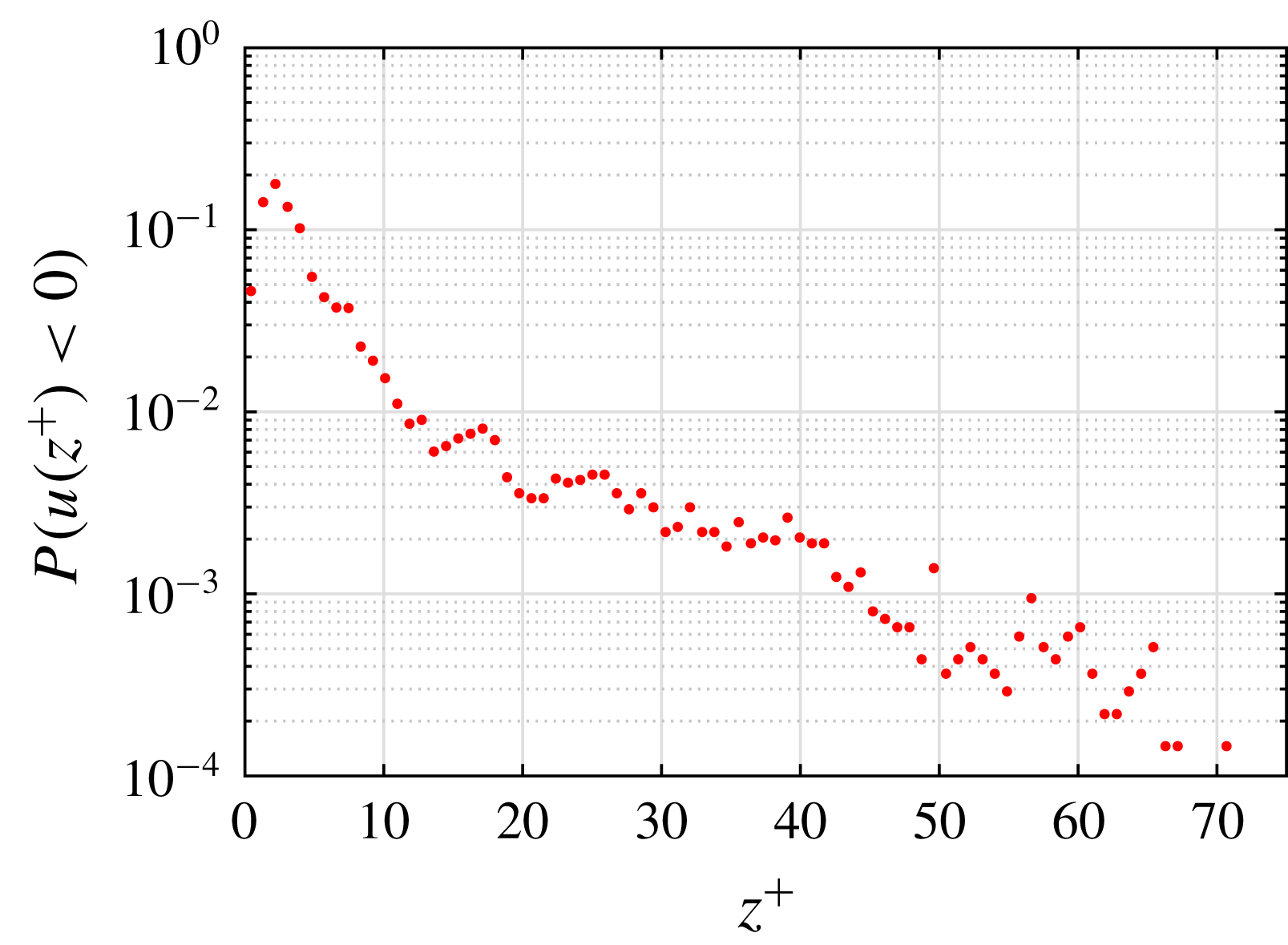
Statistically, reverse flow regions appear relatively infrequently in time (around 1.7 %). In many cases the reverse flow events only exist for a short amount of time ( ${<}50t^{+}$ ) and remain close to the wall ( $z^{+}<10$ ), e.g. at $1000{-}1500t^{+}$ . If the relative number of reverse flow events (with respect to the total number of $u<0$ ) is calculated for each wall-normal location, almost 90 % of them occur below $z^{+}=10$ as shown in figure 13. Predictably, the locations where these reverse flow events occur coincide with regions of low momentum, as the flow must be sufficiently decelerated so that the flow reversal can happen.

However, there are instances where large or extreme reverse flow events appear that persist for more than $150t^{+}$ or $4{-}5tU_{f}/\unicode[STIX]{x1D6FF}$ and extend past $z^{+}=50$ , e.g. $5500{-}5700t^{+}$ and $7500{-}7700t^{+}$ . These improbable (according to figure 13) events are shown in a zoomed in view in figure 12. In these cases, a large decelerated region appears in the surrounding flow field and extends well into the buffer and log layer. The lifetime and spatial distribution of these decelerated flow regions can be explained again by the superposition of an elongated low-momentum large-scale structure convecting on a low-speed near-wall streak. Further evidence of this large-scale structure and streak layering is evidenced by the large regions of accelerated flow, e.g. $13{-}23tU_{f}/\unicode[STIX]{x1D6FF}$ and $79{-}89tU_{f}/\unicode[STIX]{x1D6FF}$ , which can be explained by the superposition of a high-momentum large-scale structure on high-speed near-wall streaks. Therefore, it appears, based on figure 12, that under this superimposed condition large or extreme reverse flow events can take place in APG flow, which might lead to extended flow separation if the conditions are appropriate.

Figure 13.

Relative number of reverse flow events ( $u<0$ ) at a given inner scaled wall-normal location ( $z^{+}$ ) normalized by the total number of reverse flow events in an APG turbulent boundary layer at $Re_{\unicode[STIX]{x1D70F}}=2400$ ( $Re_{\unicode[STIX]{x1D70F}(ZPG)}=5000$ in the preceding ZPG section) or $Re_{\unicode[STIX]{x1D703}}=11\,500$ , and Clauser pressure gradient parameter $\unicode[STIX]{x1D6FD}=14$ .

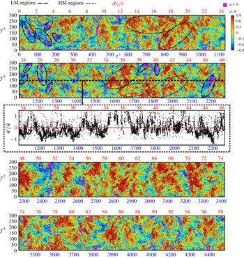
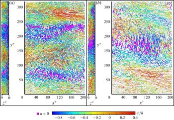
To examine this hypothesis in more detail, a 3-D measurement in the near-wall region was made. In the following discussion, near-wall features and the distribution of reverse flow events in the spanwise direction and how they are associated with the meandering near-wall streaks will be shown. As this information is embedded in the 3-D near-wall data set (3-D-TR-PTV), a corresponding space–time plot was made. In this case, trajectories passing through a wall-normal ( $z^{+}=1{-}5$ ) and spanwise ( $310y^{+}$ ) volume over a subset of the entire data set (20 000 image sequences or $4450t^{+}$ or $98tU_{f}/\unicode[STIX]{x1D6FF}$ ) is plotted in figure 14. The trajectories are coloured with the streamwise fluctuating velocity, $u^{\prime }$ , scaled with the local streamwise mean velocity, $\bar{u}$ . Reverse flow is indicated in purple where $u<0$ .

Figure 14.

Space–time plot over $t^{+}=4450$ or $tU_{f}/\unicode[STIX]{x1D6FF}=98$ , from the 3-D data set coloured with $u^{\prime }/\bar{u}$ where purple regions represent $u<0$ . Selected high-momentum (HM) and low-momentum (LM) regions are indicated in dashed ellipses.

Directly visible in this plot are the low- and high-speed near-wall streaks and the locations of reverse flow events with respect to the streaky pattern. It appears in almost all the cases shown here that the reverse flow events occur inside or at the edge of a low-speed streak, a few of which are indicated in dashed ellipses in figure 14. Furthermore, it appears that when a reverse flow event appears in a low-speed streak, that low-speed streak is often strongly tilted in the spanwise direction. This indicates the presence of streamwise oriented vortices that when slightly tilted, induce a slight flow reversal.

As observed in figure 12, in the near-wall topology there are sometimes regions of fast moving streaks that persist for $200{-}300t^{+}$ or $6{-}8tU_{f}/\unicode[STIX]{x1D6FF}$ (indicated in dashed ellipses). This can also be seen in the line plot of $u^{\prime }/\bar{u}$ for a cut through the data at $y^{+}=150$ . Although only the viscous sublayer and lower buffer layer are visualized there, this extended region of fast moving streaks is consistent with the lifetime of the superposition of large-scale structures and streaks shown in figure 12. What is also visible is the appearance of groupings for reverse flow events, distributed in the spanwise direction, e.g. between $0{-}250t^{+}$ and $1150{-}1300t^{+}$ . As established in figure 12, in order for these groupings to occur, the flow in the near-wall and far field regions must be sufficiently decelerated. This is achieved if a low-momentum large-scale structure is superimposed on a near-wall low-speed streak. In other words, groupings of reverse flow events can occur only when the flow is sufficiently decelerated by the layering of a low-speed near-wall streak and an elongated low-momentum large-scale structure in the far field. However, as this situation is often fulfilled, the question arises as to whether another event must take place simultaneously to make reverse flow events possible. A statistical analysis of these topological and dynamic features is provided in the next section.

8 Statistics of reverse flow events

8.1 Reverse flow detection

In the following sections a deeper statistical analysis of the reverse flow events is presented in order to quantitatively characterize their occurrence frequency, connection with other events and preferred orientation in the spanwise direction.

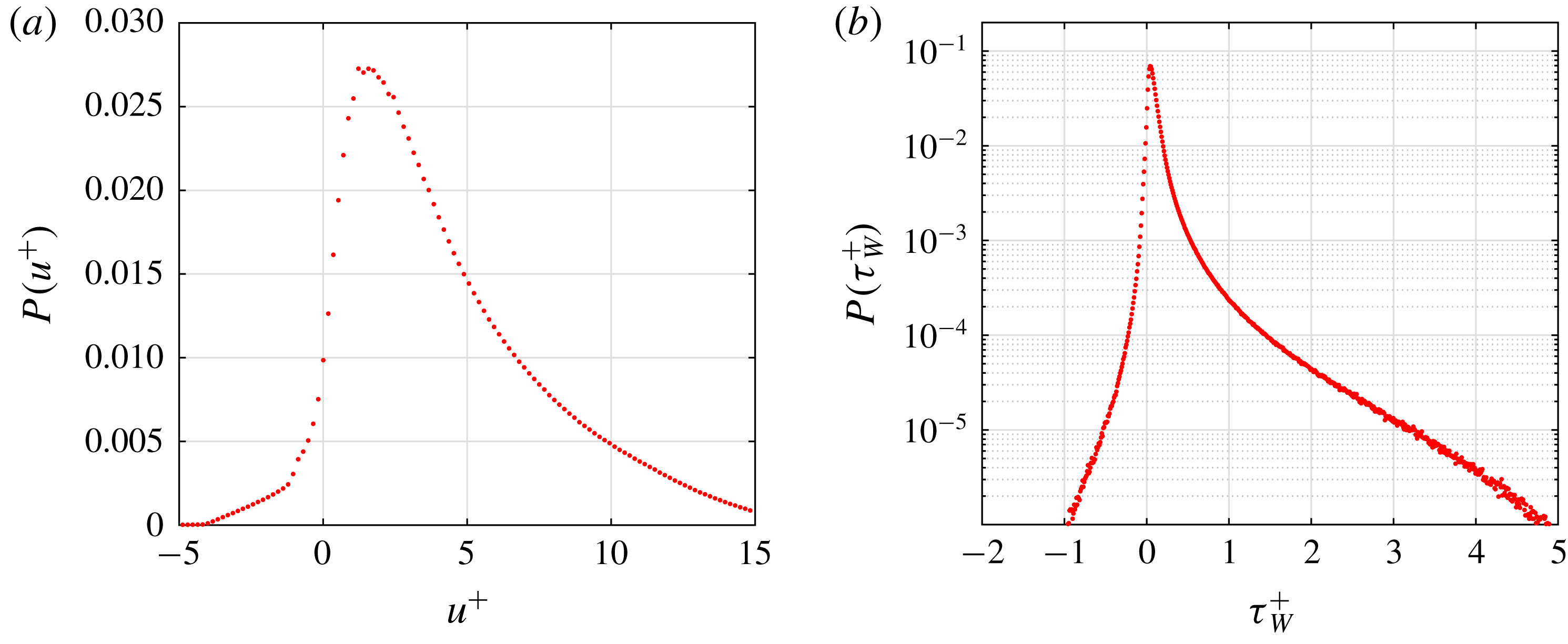
The probability of reverse flow events based on the distribution of the instantaneous streamwise velocity is shown in figure 15(a). In this plot the maximum probability occurs at a $u^{+}=1.5$ and sharply decreases in the $u^{+}<0$ region. In this case, the probability of reverse flow calculated by summing the region for $u^{+}<0$ or $\unicode[STIX]{x1D70F}_{W}<0$ in figure 15(a) or 15(b), is 0.017 or 1.7 %. This value represents a much larger value than presented in other measurements for a ZPG boundary layer and channel flow (Lenaers et al. Reference Lenaers, Li, Brethouwer, Schlatter and Örlü2012; Willert Reference Willert2015; Willert et al. Reference Willert, Cuvier, Foucaut, Klinner, Stanislas, Laval, Srinath, Soria, Amili and Atkinson2018). However, in the DNS channel flow computation in Lenaers et al. (Reference Lenaers, Li, Brethouwer, Schlatter and Örlü2012), an increase in reverse flow probability for increasing $Re_{\unicode[STIX]{x1D70F}}$ up to 1000 was reported. Furthermore, an increase in reverse flow probability was also reported for increasing APG conditions in Vinuesa et al. (Reference Vinuesa, Örlü and Schlatter2017b ), which is intuitive as more flow reversal is expected as separation is approached. Therefore, the relatively large reverse flow measured herein at $Re_{\unicode[STIX]{x1D70F}}=2400$ ( $Re_{\unicode[STIX]{x1D70F}(ZPG)}=5000$ in the preceding ZPG section) for a turbulent boundary layer with APG conditions is in accordance with the trends reported in the aforementioned DNS studies. However, different upstream pressure gradient development histories over a wing and an APG turbulent boundary layer (preceded by a long ZPG) at matched $\unicode[STIX]{x1D6FD}$ can result in mean wake and Reynolds stresses differences (Bobke et al. Reference Bobke, Vinuesa, Örlü and Schlatter2017) and can also contribute to differences in reverse flow event statistics.

Nevertheless, we can conclude that the existence of reverse flow events is not a low Reynolds numbers effect as they also appear at the relatively high Reynolds number investigated herein. As the magnitude of the near-wall velocity fluctuations is associated with the rising intensity of the turbulent superstructures with Reynolds number, and the fact that the superstructures modulate the near-wall features according to figures 7(a), 7(b) and 8, the number of reverse flow events is expected to increase with increasing Reynolds number. However, due to the strong velocity gradient in the wall-normal direction, their extension in the in $z$ -direction reduces, as shown in figure 13. This makes their measurement at large Reynolds number more difficult due to spatial resolution limitations. However, in the analysis all reverse flow events can be reliably resolved.

Figure 15.

(a) Inner scaled instantaneous streamwise velocity ( $u^{+}$ ) and (b) inner scaled instantaneous wall shear stress ( $\unicode[STIX]{x1D70F}_{W}$ ) probabilities, from 3-D-TR-PTV measurements for $z^{+}<$ 8 in an APG turbulent boundary layer at $Re_{\unicode[STIX]{x1D70F}}=2500$ ( $Re_{\unicode[STIX]{x1D70F}(ZPG)}=5000$ in the preceding ZPG section) or $Re_{\unicode[STIX]{x1D703}}=12\,000$ , and Clauser pressure gradient parameter $\unicode[STIX]{x1D6FD}=13.5$ .

The low probability of reverse flow can also be illustrated by calculating the instantaneous wall shear stress. Taking advantage of the high spatial resolution in the viscous sublayer, the wall shear stress, $\unicode[STIX]{x1D70F}_{W}=\unicode[STIX]{x1D707}\unicode[STIX]{x2202}u/\unicode[STIX]{x2202}z|_{z=0}$ , can be directly calculated. The probability distribution function for the inner scaled wall shear stress is provided in figure 15(b) for completeness. This plot is more relevant than plot 15(a) as the distribution of the wall shear stress does not depend on the height of the measurement volume.

In the aforementioned discussion and figures the probability of individual reverse flow trajectories of tracer particles was considered. However, it must be kept in mind that a reverse flow event is comprised of many tracer particles and therefore the occurrence probability of a reverse flow event (one large event comprised of many tracer particles) is actually much smaller, as will be discussed in § 8.4.

8.2 Reverse flow and extreme wall-normal events

Another feature of the near-wall region worth studying is the connection between extreme flow events and a strong wall-normal velocity. These events, which are associated with the sweep ( $u^{\prime }>0$ , $w^{\prime }<0$ or $Q4$ ) and ejection ( $u^{\prime }<0$ , $w^{\prime }>0$ or $Q2$ ) of the near-wall streaks have been well documented and discussed in the literature (see review Wallace (Reference Wallace2012)). In this section, the connection of extreme wall-normal fluctuations and the reverse flow will be explored in order to determine if there is a link between them. In figure 16(a) the probability density function of the instantaneous wall-normal velocity, $w$ , normalized by the root mean square $w_{rms}$ is shown. In this plot, the probability of fluctuations beyond $\pm 8w_{rms}$ is several orders of magnitude lower than their maximum and therefore events outside of this range will be referred to as extreme events.

To examine the connection of wall-normal fluctuations and reverse flow events a joint probability function (j.p.d.f.) of $u/u_{rms}$ and $w/w_{rms}$ is plotted in 16(b). In this figure it appears that there is not a strong correlation between extreme wall-normal events (beyond $\pm 8w_{rms}$ ) and reverse flow events ( $u/u_{rms}<0$ ), which is in agreement with DNS results at lower Reynolds number (Lenaers et al. Reference Lenaers, Li, Brethouwer, Schlatter and Örlü2012; Vinuesa et al. Reference Vinuesa, Örlü and Schlatter2017b ). This shows that reverse flow events are a typical feature of the flow that are not connected to extreme wall-normal events. Therefore, there must be another responsible reason for their low occurrence probability.

Figure 16.

(a) Wall-normal fluctuation probability density function (p.d.f.) and (b) joint probability density function (j.p.d.f.) of wall-normal and streamwise velocities normalized with their root mean square.

8.3 Flow direction statistics

The previous analysis showed the characteristics of reverse flow events, i.e. their size, extent in the wall-normal direction and dynamics. Furthermore, it was shown that reverse flow events are not connected with extreme wall-normal events. Therefore, in this section the orientation of reverse flow motion is analysed; specifically their connection to spanwise motion, which could already be seen qualitatively in figure 14. To examine if there is a connection between reverse flow events and strong spanwise motion, the flow direction based on the $u$ and $v$ vector components (the wall-normal velocity component has little effect when compared to the other components) is calculated. In order to separate more extreme events the data set is conditioned into two groups with $|\unicode[STIX]{x1D70F}_{W}|>\unicode[STIX]{x1D70F}_{W,rms}$ and $|\unicode[STIX]{x1D70F}_{W}|<\unicode[STIX]{x1D70F}_{W,rms}$ . The probability at each angle for each conditioned set is provided in figure 17. In these plots, $0^{\circ }$ and $360^{\circ }$ degrees indicate flow in the positive $x$ -direction and $180^{\circ }$ is flow purely in the negative $x$ -direction. For each case the flow direction with the lowest probability was used to normalize the rest of the probabilities which are then scaled logarithmically. It must be noted that the conditioning requirement, $|\unicode[STIX]{x1D70F}_{W}|>\unicode[STIX]{x1D70F}_{W,rms}$ , reduces the data set to only 35 % of the original set. Nonetheless, the preferred flow direction of these more intense events will provide insight into the larger turbulent action of the flow in the near-wall region.

Figure 17.

Logarithmically scaled flow direction probabilities for (a)  $|\unicode[STIX]{x1D70F}_{W}|>\unicode[STIX]{x1D70F}_{W,rms}$ and (b)  $|\unicode[STIX]{x1D70F}_{W}|<\unicode[STIX]{x1D70F}_{W,rms}$ .

In figure 17(a), where $|\unicode[STIX]{x1D70F}_{W}|>\unicode[STIX]{x1D70F}_{W,rms}$ , the flow directions with the lowest probability occur at $90^{\circ }$ and $270^{\circ }$ , see figure 17(a). Relative to the probability at $90^{\circ }$ and $270^{\circ }$ , the flow is almost two orders of magnitude more likely to travel in the $180^{\circ }$ direction. Therefore, it seems for these more intense fluctuations, the flow direction is most likely to have an upstream orientation during a reverse flow event. This was also seen in the DNS study for strong APG conditions in Vinuesa et al. (Reference Vinuesa, Örlü and Schlatter2017b ). However, when looking at the other conditioned set of $|\unicode[STIX]{x1D70F}_{W}|<\unicode[STIX]{x1D70F}_{W,rms}$ , which represents a much larger portion of the data set, a different distribution is present. In figure 17(b), the least likely probability occurs at $180^{\circ }$ and the reverse flow for these fluctuations are more likely to have a strong spanwise component. This implies that reverse flow events of this type are associated with small streamwise vortex filaments that are close to the wall and slightly tilted with respect to the main flow direction.

Therefore, it becomes evident based the analysis in the previous sections that reverse flow events become possible if turbulent superstructures, near-wall low-speed streaks and vortex filaments inside or near decelerated near-wall low-speed streaks interact in a specific manner. First, the low-speed streaks near the wall must be sufficiently retarded by low-momentum large-scale superstructure. Second, near-wall vortex filaments with the right attributes, i.e. distance to the wall and intensity, present in the vicinity of the retarded low-speed streaks, can cause reverse flow events. This complex interaction between the coherent flow motions explains why the reverse flow events are so rare.

8.4 Reverse flow event lifetime

According to the generation mechanism of reverse flow events outlined in the last section, it is understandable why these events are so rare. In this section the distribution and spacing of reverse flow events in time is addressed. Figure 18 shows the distribution of reverse flow events in time, where trajectories with $u<0$ are grouped into bins of 50 time sequences.

Many intervals exist where almost no reverse flow events are detected. This is expected because when high-momentum large-scale structures convect through the measurement plane no events are possible according to the interaction model previously mentioned. Secondly, it appears that reverse flow events often appear in groups. This does not necessarily mean that they interact in these groups, but it seems that once a reverse flow event is detected, finding more events within a short time period is likely. This is evident from the model, i.e. when the right conditions are generated reverse flow event appearance becomes likely. By using analysis of this type, it is possible to locate image ranges where significant reverse flow occurs. Furthermore, if one considers the probability of major reverse flow events (bins with amplitudes larger than 2000), it is one order of magnitude less than previously calculated for individual reverse flow vectors, i.e. 0.1 % compared to 1.7 %. If the events seen in the 2-D data set are counted from figure 12 in this way, a similar percentage of 0.15 % of reverse flow events is measured.

Figure 18.

Reverse flow event detection over a time series, from 3-D-TR-PTV fields.

The lifetime of large events is around 10–20 ms or $24t^{+}$ to $48t^{+}$ where $t^{+}=(tu_{\unicode[STIX]{x1D70F}}^{2}/\unicode[STIX]{x1D708})$ but they can appear one after the other in a low-speed streak for up to and beyond 100 ms (or $240t^{+}$ ).

9 Reverse flow event visualization

In the following section, trajectory plots for a few of the extreme reverse flow events are provided. This is done to not only visualize the topology of these events but also further demonstrate the connection between reverse flow events and low-speed near-wall streaks, low-momentum superstructures and tilted longitudinal vortices.

In figure 19 a sequential set of flow trajectories during one of the large reverse flow events identified in figure 12 is shown in physical space with streamwise velocity colouring. In this case, each plot ( $t1,t2,\ldots$ ) represents particle trajectories over 100 image sequences ( $28.1t^{+}$ ). Highlighted in purple are reverse flow vectors. What can be seen in this sequence is the continued deceleration of the flow in the wall-normal direction (from $t1$ to $t3$ ) due the presence of a low-momentum superstructure, which sufficiently decelerates the near-wall flow allowing for the large flow reversal shown in plots $t4$ and $t5$ . After this sequence of course the reverse bubble remains close to the wall (in $t6$ and $t7$ ) while the outer flow accelerates until the flow reversal disappears in $t9$ . This would mean the convection velocity of this large reverse flow event bubble is around $0.5u^{+}$ which corresponds to a streamwise length of around 95 viscous units. This is longer than the average streamwise extension of reverse flow events of around $20x^{+}$ in Willert et al. (Reference Willert, Cuvier, Foucaut, Klinner, Stanislas, Laval, Srinath, Soria, Amili and Atkinson2018) for a ZPG turbulent boundary layer and in Vinuesa et al. (Reference Vinuesa, Örlü and Schlatter2017b ) for turbulent flow over a wing, which is likely due to the fact that we are considering extreme events in a APG turbulent boundary layer. However, as indicated in figures 13 and 18, a variety of reverse flow events are detected in terms of their lifetime and extension in the wall-normal direction. Which suggests that a collection of reverse flow events exist in the strong APG flow considered in this investigation that have different convection velocities and sizes in the streamwise direction.

Furthermore, a selection of reverse flow events based on the maximum amplitude of the peaks in figure 18 are visualized in figure 20 by plotting three-dimensional trajectories coloured with $u^{\prime }/\bar{u}$ . With this colour coding, regions of low and high momentum with respect to the mean velocity can be quantitatively determined. Reverse flow, i.e. $u<0$ , is again highlighted in purple. A movie showing a short sequence of the three-dimensional near-wall flow can be found in the supplementary material (movie 2).

Figure 19.

Two-dimensional trajectories during an extreme instantaneous reverse flow event in an APG turbulent boundary layer at $Re_{\unicode[STIX]{x1D70F}}=2400$ ( $Re_{\unicode[STIX]{x1D70F}(ZPG)}=5000$ in the preceding ZPG section) or $Re_{\unicode[STIX]{x1D703}}=11\,500$ , and Clauser pressure gradient parameter $\unicode[STIX]{x1D6FD}=14$ . Trajectories are coloured with $u^{\prime }/\bar{u}$ , where positive flow is from left to right. Also highlighted are regions of $u<0$ . Each plot ( $t1,t2,\ldots$ ) represents particle trajectories over 100 image sequences ( $28.1t^{+}$ ).

In figure 20(a) shows trajectories over a time series of 100 images ( $28.4t^{+}$ ). Two views of the volume are shown, one in the $xy$ plane and also a view looking at the volume from the left side of the $xy$ plot in the $zy$ plane. For this particular case, the streaky structure of low- and high-speed streaks is immediately obvious. Also visible are $u<0$ events distributed in the regions of low speed. Looking at the $xy$ view, these reverse flow events are present in a group in the near-wall low-speed streaks across the entire streamwise extent of the measurement volume, or approximately 150 viscous lengths. Moreover, the long streamwise extent of the low-speed streaks explains why the reverse flow events can be observed in packages.

Figure 20.

Three-dimensional trajectories during two different (a and b) instantaneous reverse flow events in an APG turbulent boundary layer at $Re_{\unicode[STIX]{x1D70F}}=2500$ ( $Re_{\unicode[STIX]{x1D70F}(ZPG)}=5000$ in the preceding ZPG section) or $Re_{\unicode[STIX]{x1D703}}=12\,000$ , and Clauser pressure gradient parameter $\unicode[STIX]{x1D6FD}=13.5$ . Trajectories are coloured with $u^{\prime }/\bar{u}$ , where positive flow is from left to right. Also highlighted are regions of $u<0$ .

To highlight that the topology of these reverse flow events is not universal as discussed in § 8.3, another set (independent of (a)) of instantaneous trajectories is plotted on the right, (b), side of figure 20. In contrast to (a), the flow is dominated by one large spanwise ( $y$ -direction) directed event. Trajectories with $u<0$ appear grouped in a defined spatial location and extend over and area of $120\times 120$ viscous lengths in the streamwise and spanwise directions, which is much larger than the spanwise extent of the low-speed streaks shown in (a). Furthermore, the significant spanwise motion of this flow event was not observed to this extent in (a).

Considering the results presented here, it is evident that the large spanwise motion must be associated with a slightly titled longitudinal vortex, as previously reported in Lenaers et al. (Reference Lenaers, Li, Brethouwer, Schlatter and Örlü2012) and Diaz-Daniel et al. (Reference Diaz-Daniel, Laizet and Vassilicos2017). This is confirmed by the cross-plane visualization ( $zy$ view). If the axis of a streamwise vortex is slightly tilted with respect to the mean flow direction due to the meandering of the vortices, these longitudinal vortices can generate reverse flow events, provided the vortex travels with a sufficiently low convection velocity, which is possible when the vortex is sufficiently strong, located close to the wall and embedded inside a low-speed streak. Consequently, this generation mechanism is based on a interaction between low-speed streaks and tilted streamwise vortices. If the local convection velocity is increased locally by high-speed large-scale superstructures, reverse flow events are fully suppressed and cannot appear, as discussed in previous sections and shown in figures 12 and 14.

10 Concluding remarks

The work presented herein investigates the coherent flow motions in an adverse pressure gradient turbulent boundary layer following a zero pressure gradient turbulent boundary layer at $Re_{\unicode[STIX]{x1D70F}}=5000$ with a novel time-resolved volumetric PTV technique developed by the authors. This technique is able to determine with high spatial resolution, low uncertainty and without bias errors (due to spatial averaging for instance) the flow velocity within the buffer and viscous sublayer. Furthermore, time-resolved particle tracking measurements were performed in a single wall-normal slice in order to measure over long times the interaction of the turbulent superstructures with the near-wall flow motions down to the viscous sublayer.

Using the information in time and space, it was confirmed directly that the superstructures modulate the near-wall flow all the way down to the viscous sublayer. The modulation of the wall shear stress is therefore determined by the length, intensity and frequency of the superstructures and scales with outer units. The analysis of the space–time correlations show that the near-wall motion responds to the influence of the outer layer motion with a characteristic time shift. This is due to the forward leaning nature of the large-scale structures.

Due to the high spatial resolution of the measurements near the wall, characteristic uniform-momentum zones could be resolved in the viscous sublayer, throughout the buffer layer and up to the log-law region. Due to the fact that the near-wall streaks and the superstructures exist in low-, neutral- and high-momentum form, their superposition can lead to various UMZ patterns or layering. Taking also into account that the height of the coherent structures varies the thickness of each UMZs layer can be quite different in space and time. Furthermore, as the coherent structures meander quite strongly, they appear with a characteristic tilt or as shear layers with a characteristic angle if the measurement plane slices the structures at an angle, which is usually the case in planar PIV/PTV experiments.

It was shown that the reverse events appear in a region of low-momentum fluid extending from the wall to the log layer for this strong adverse pressure gradient turbulent boundary layer. For turbulent channel or boundary layers with little or low pressure gradients, reverse flow events have only been reported close to the wall, $z^{+}<5$ (Lenaers et al. Reference Lenaers, Li, Brethouwer, Schlatter and Örlü2012; Willert Reference Willert2015; Willert et al. Reference Willert, Cuvier, Foucaut, Klinner, Stanislas, Laval, Srinath, Soria, Amili and Atkinson2018). Nevertheless, this illustrates that the deceleration of the near-wall low-speed streaks by low-momentum superstructures is very important for the generation of reverse flow events. Furthermore, if reverse flow events appear, they are often followed by a sequence of events because if a low-momentum superstructure decelerates a low-speed streak sufficiently the conditions are appropriate for the appearance of reverse flow events. However, if a high-momentum superstructure is present in the observation plane, reverse flow events cannot be detected. This explains why the reverse flow events appear often in ‘packages’ or in a sequence. In addition, it was observed that most of the reverse flow events remain below $z^{+}=10$ . However, at least two extreme cases were observed where large reverse flow regions occurred over many times steps that penetrate into even the log-law layer. These large reverse flow events can extend in both spanwise and streamwise directions up to ${\sim}100$ viscous units, which is larger than the dimensions given in the literature for the ZPG case at lower Reynolds numbers. Which may suggest that reverse flow events might trigger large-scale flow separations if the conditions are appropriate.

It is evident from the analysis that low-speed streaks are a necessary condition for the existence of reverse flow events. Another necessary condition is the deceleration of the low-speed streak by low-momentum superstructures. However, this condition is realized quite often in the flow and therefore the question arises as to why the reverse flow events are seen so seldom. A detailed analysis of the measurements has shown evidence of small longitudinally oriented vortices generating spanwise directed trajectories in the vicinity of reverse events. The probability of the majority of reverse flow vectors having a significant spanwise component was shown to be much more likely than reverse events directed purely in the upstream direction, which is induced by the spanwise or wall-normal vortices. However, these kind of reverse flow events only occur when the axis of the streamwise vortices is slightly tilted with respect to the mean flow direction, generating flow in both the spanwise and upstream (reverse) directions.

The results clearly show that reverse flow events are not necessarily unique in terms of the topology and temporal frequency and it is evident that these differences are linked with the strength of the fluctuating near-wall flow. It was also demonstrated that reverse flow events are not strongly correlated with extreme wall-normal events, which perhaps provides further insight into dynamics of the near-wall flow. However, whenever the specific conditions are reached, i.e. sufficient deceleration of the near-wall low-speed streaks by low-momentum superstructures, multiple reverse flow events were shown to appear one after another if the interaction with a tiny near-wall vortex of sufficient strength takes place. Therefore, the following conceptual model, shown in figure 21, illustrates the possibility of reverse flow events based on the topological and statistical analysis presented herein.

Figure 21.

Conceptual model indicating the spatial distribution and interaction of coherent flow structures that lead to reverse flow events.

1. (i) Low-speed near-wall streaks (dark blue) must be sufficiently decelerated by superimposed low-momentum large-scale superstructures (light blue).

2. (ii) Streamwise vortex filaments of sufficient intensity must be present at small wall distances and they must be located inside or near the retarded low-speed streaks to produce a sufficiently strong spanwise motion. When these particular vortices are slightly tilted with respect to the streamwise direction due to the meandering of the streaks for instance, they can produce reverse flow with a significant spanwise velocity component.

3. (iii) Spanwise vortices located at the retarded near-wall low-speed streaks can also produce reverse flow events but with a strong reverse flow component and only a small spanwise flow component.

4. (iv) The complex interaction of (i) and either (ii) or (iii) to generate reverse flow events explains why reverse flow events are quite rare. However, as (iii) is more dominant in high APG flows, reverse flow events become more common in these flows.

5. (v) If the near-wall flow is not strongly decelerated by low-momentum superstructures, reverse flow events are not possible. Which explains why there are large time intervals where no reverse flow events occur.