2. MEASUREMENT MODELS OF SLR AND CBTR

The instantaneous observations of SLR and CBTR can be expressed as (t, ρ _Si ), (t, ρ _Ci ) respectively. They can be defined as

(1) $$\left\{ {\matrix{ \matrix{\!\!\!\!\!\!\!\!\!\!\!\rho _{Si} = \rho _{SCi} + \Delta \rho _{STPE} + \Delta \rho _{SOFC} + \Delta \rho _{SDEL} + \Delta \rho _{SRLA} \hfill \cr \;+ \Delta \rho _{STRO} + \Delta \rho _{SOFF} + \Delta \rho _{SNOI}\matrix{ {\matrix{ {} & {} & {} \cr } } & {} & {} & {} \cr } \hfill} \cr \matrix{\rho _{Ci} = \rho _{CCi} + \Delta \rho _{CTPE} + \Delta \rho _{COFC} + \Delta \rho _{CDEL} + \Delta \rho _{CRLA} \hfill \cr \quad \quad \; + \Delta \rho _{CTRO} + \Delta \rho _{COFF} + \Delta \rho _{CNOI} + \Delta \rho _{CION} + \Delta \rho _{CTRA} \hfill} \cr } } \right.$$

where t is the instantaneous observation time, ρ _Si is the SLR range between SLR station and satellite, ρ _Ci is the C-Band pseudo-range between C-Band station and satellite and ρ _SCi and ρ _CCi are the geometrical distances between SLR, C-Band station and satellite, respectively. Δρ _STPE and Δρ _CTPE are the corrections due to tectonic plate movements, solid-Earth tides, ocean tide loading and the Earth's rotational deformation. The station coordinate changes caused by solid-Earth tides and ocean tide loading can be calculated by applying the Wahr model (Wahr, Reference Wahr1981; Li, Reference Li1995), the Schwlderski 1978 model and Green's function (Melbourne et al., Reference Melbourne, Anderle, Fessiel, King, McCarthy, Smith, Tapley and Vicente1983; Li, Reference Li1995), with the changes caused by Earth rotation referred to the International Earth Rotation and Reference Frame Service (McCarthy and Petit, Reference McCarthy and Petit2004).

Δρ _SOFC and Δρ _SDEL are the centre corrections of the SLR site and the time delay of the laser ranging instruments. In order to obtain accurate observations, these two items can be calibrated by the shooting method (Zhang et al., Reference Zhang, Yang and Chen1990; Zhao et al., Reference Zhao, Pan, Wang and Luo2010). Usually, these two corrections have been deducted from the SLR observations by the International Laser Ranging Service (ILRS) analysis.

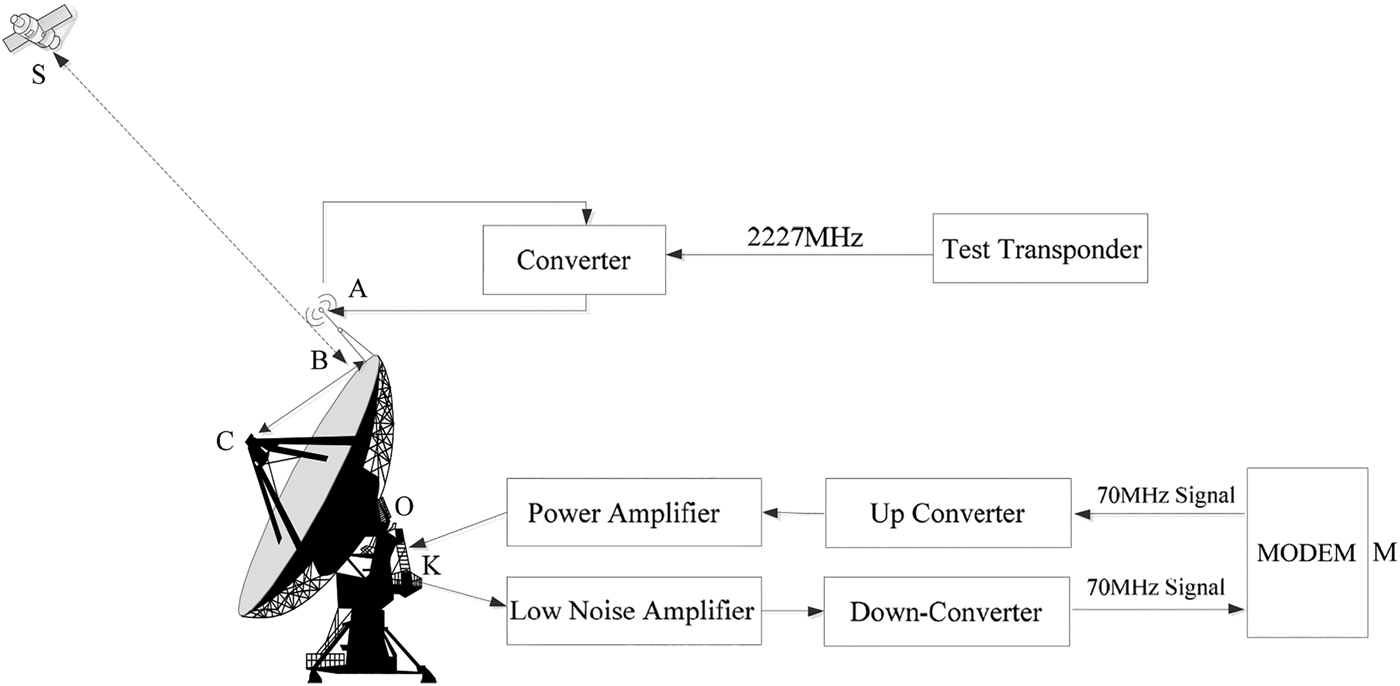
Δρ _COFC and Δρ _CDEL are the centre corrections of the C-Band station antenna phase and the time delay in the station instruments. Similar to SLR, these two items are also measured in the first ten minutes of every hour. During data-processing, this time delay can be eliminated from the CBTR observations. The station instruments contain the modem, up/down converters, power amplifier, low noise amplifier, the cable and so on (Figure 1). Point O depicts the centre of the C-Band station, being the cross of the pitch and the azimuth indicators. Points M, K and C depict the modem, feed network and the centre of the sub-reflector. Points A and S depict the phase centre of the satellite simulator and the satellite transponder. The station delay measurement process is as follows. The up signal from the modem with 70 MHz frequency passes through the up converter with its frequency changing to 6 GHz. Then the signal is transmitted by the C-Band antenna and can be converted to a 4 GHz signal by the satellite simulator using the test transponder at the antenna edge (as B). Finally the signal can be received by the C-Band antenna again and passes through a low noise amplifier, a down converter changing the frequency to 70 MHz before the signal is received by the modem. The station delay contains the test transponder delay, which does not belong to the real signal. However, it is difficult to measure the test transponder delay. Therefore, there would be biases in the data participating in POD when these two items are measured wrongly.

Figure 1.

The delay measurement at a CAPS station.

Δρ _SRLA and Δρ _CRLA are the corrections of general relativistic effects, which can be corrected using the Shapiro Reference Shapiro1964 model (Shapiro, Reference Shapiro1964).

Δρ _STRO and Δρ _CTRO are the corrections of the tropospheric delays for the SLR and C-Band signals, respectively. For SLR, the delay can be corrected by applying the Marini-Murray model (Marini and Murray, Reference Marini and Murray1973). For the CBTR signal, the delay can be corrected by applying the Saastamonien Reference Saastamonien1973 model (Saastamonien, Reference Saastamonien1973) and the Niell mapping function (Niell, Reference Niell1996), which can be used to calculate the delay in zenith and observation direction, respectively (Cao et al., Reference Cao, Yang, Su, Li, Chen, Li, Sun, Kong, Wei and Feng2014b).

Δρ _SOFF and Δρ _COFF are the corrections from the SLR reflector and phase centre of the on board transponder to the satellite barycentre, respectively.

Δρ _SNOI and Δρ _CNOI are the random noises in SLR and CBTR observations.

Δρ _CION and Δρ _CTRA are the corrections of the ionospheric and transponder delays (Cao et al., Reference Cao, Yang, Su, Li, Chen, Li, Sun, Kong, Wei and Feng2014b). They are contained in the CBTR but not in the SLR observations. Though the transponder delay can be measured before satellite transmission, there is still some uncertainty as neither the test transponder delay nor the value cannot be obtained from data-processing. Therefore, the transponder delay is always treated as a parameter to be solved. Moreover, there is the model bias in the ionospheric delay calculation.

Since the centre corrections of the SLR site and the time delay of laser ranging instruments have been deducted from the SLR observations in the ILRS solutions, and the random noise of SLR is small, Equation (1) can be simplified to Equation (2).

(2) $$\left\{ {\matrix{ \hskip -19pt {\rho _{Si} = \rho _{SCi} + \Delta \rho _{STPE} + \Delta \rho _{SRLA} + \Delta \rho _{STRO} + \Delta \rho _{SOFF}} \cr \matrix{\rho _{Ci} = \rho _{CCi} + \Delta \rho _{CTPE} + \Delta \rho _{CRLA} + \Delta \rho _{CTRO} + \Delta \rho _{COFF} \hfill \cr \hskip 24pt + \Delta \rho _{CNOI} + \Delta \rho _{COFC} + \Delta \rho _{CDEL} + \Delta \rho _{CION} + \Delta \rho _{CTRA} \hfill} \cr } } \right.$$

From Equations (1) and (2), we can see that the station delay bias, the transponder delay bias, the ionospheric delay model bias and other biases perform the same function to the measurement equation. For each station, it is the sum of these biases that needs to be calibrated as it is difficult to separate them into their individual contributions.

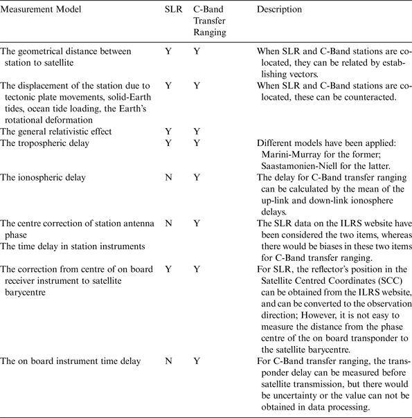
Table 1 gives the similarities and differences between SLR and CBTR. The ‘Y’ means that the item in the row is associated with the item in the column. ‘N’ means that the item in the row is not associated with the item in the column. Thus Table 1 shows which signal biases in CBTR observations can be calibrated using SLR data. When SLR and C-Band stations are co-located, the signal propagation path, the displacement of the station and the general relativistic effect can be assumed to be identical and cancelled out for SLR and CBTR. The co-location comparison method can be employed for signal biases calibration. If the stations cannot be co-located, the combined POD method can be employed to calibrate the signal biases.

Table 1.

The similarities and differences between SLR and C-Band transfer ranging.

3. THE SIGNAL BIASES CALIBRATION OF CAPS USING SLR AND CBTR

Being affected by weather and limited to tracking a Geostationary Earth Orbit (GEO) satellite at a height of 36000 km, only a few SLR sites can observe the GEO satellite with CAPS C-Band stations located in Changchun, Linton and Kashi simultaneously, resulting in few co-observations of SLR and CAPS. Only observations from the Changchun SLR site and CAPS C-Band stations were obtained on 12 April, 14, 16 and 24 May 2011. Moreover, co-observations were obtained again on 6, 13, 15, 17 and 23 July, and 5 August 2012. Therefore, the signal biases of the Changchun C-Band station can be calibrated using the co-location comparison method. Then, the biases for the other two C-Band stations can be calculated by the combined POD method.

3.1. The signal biases calibration for the Changchun C-Band station using the co-location comparison method

When the SLR site and C-Band station are situated at the same place and the same GEO satellite with a laser reflector is observed by these two measurements simultaneously, the co-location comparison method can be used. After the pre-processing of SLR and C-Band observations in the same observing arc, the signal biases can be obtained using the GEO satellite orbit by SLR, azimuth and elevation observations.

Firstly, the SLR instantaneous ranging/azimuth/elevation observations (Li, Reference Li1995) and CBTR instantaneous observations by transfer should be prepared. The C-Band instantaneous observations (Liu et al., Reference Liu, Zhang and Wu2007) by transfer at the SLR observation time can be formulated by interpolation of the C-Band observation time.

Secondly, the GEO satellite orbit should be obtained by SLR instantaneous ranging observations in company with azimuth and elevation observations, with ranging residuals Root Mean Square (RMS) being better than 2 cm.

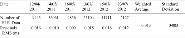
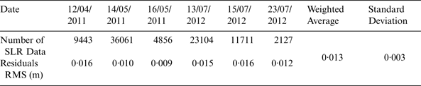
The co-observations of the BeiDou satellite (COSPAR ID 2010-001A) using the Changchun SLR site and CBTR station were collected in April 2011, May 2011 and July 2012. Table 2 shows the statistics of the residuals for the SLR observations in POD of SLR observations. From Table 2, the residuals RMS of SLR ranging observations is about 0·013 m, with standard deviation being 0·003 m. Thus the GEO satellite orbit can be fitted well to SLR ranging observations.

Table 2.

Statistics of the residuals for the SLR observations in POD of SLR observation.

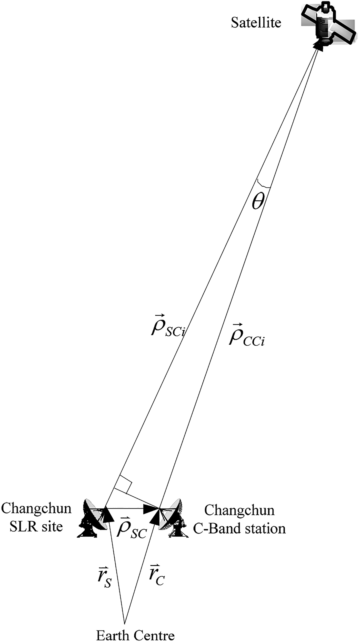
After the GEO orbit has been obtained, the signal biases for the Changchun C-Band station can be calibrated using the co-location comparison method, since they are about 40 m apart. Figure 2 shows the Earth-Fixed Coordinate System vectors for the co-location method. ${\mathop {\rho} \limits{{\hskip-8pt}^\rightharpoonup}}_{\hskip-2pt SCi} $ and ${\mathop {\rho} \limits{{\hskip-8pt}^\rightharpoonup}}_{\hskip-2pt CCi} $ are the instantaneous geometrical vectors from the SLR and CBTR station to the satellite, respectively. ${\mathop {r} \limits{{\hskip-8pt}^\rightharpoonup}}_{\hskip-2pt S} $ and ${\mathop {r} \limits{{\hskip-8pt}^\rightharpoonup}}_{\hskip-2pt C} $ are the coordinate vectors of the Changchun CBTR station and SLR site, respectively. ${\mathop {\rho} \limits{{\hskip-8pt}^\rightharpoonup}}_{\hskip-2pt SC}$ is the instantaneous vector from the SLR site to the C-Band station, which can be obtained from ${\mathop {\rho} \limits{{\hskip-8pt}^\rightharpoonup}}_{\hskip-2pt SC} = {\mathop {r} \limits{{\hskip-8pt}^\rightharpoonup}}_{\hskip-2pt C} - {\mathop {r} \limits{{\hskip-8pt}^\rightharpoonup}}_{\hskip-2pt S}$ .

Figure 2.

Depiction of co-location comparison method of the Changchun C-Band station.

Because of the co-location, the station displacements and the general relativistic effects can be assumed to be identical and cancelled out for SLR and CBTR. Equation (2) can be rewritten as Equation (3).

(3) $$\left\{ {\matrix{ \hskip -65pt {\rho _{Si} = \rho _{SCi} + \Delta \rho _{STRO} + \Delta \rho _{SOFF}} \cr \matrix{\rho _{Ci} = \rho _{CCi} + \Delta \rho _{CTRO} + \Delta \rho _{COFF} + \Delta \rho _{CNOI} \hfill \cr \quad \quad \;+ \Delta \rho _{COFC} + \Delta \rho _{CDEL} + \Delta \rho _{CION} + \Delta \rho _{CTRA} \hfill} \cr } } \right.$$

In order to obtain the relation between SLR and CBTR data, ${\mathop {\rho} \limits{{\hskip-8pt}^\rightharpoonup}}_{\hskip-2pt SC} $ , ${\mathop {\rho} \limits{{\hskip-8pt}^\rightharpoonup}}_{\hskip-2pt CCi}$ can be projected to the direction of ${\mathop {\rho} \limits{{\hskip-8pt}^\rightharpoonup}}_{SCi} $ . The cosine of θ is near to 1, since the two stations are co-located. The relation between the two types of data can be expressed as Equation (4).

(4) $$\rho _{SCi} = \rho _{CCi} + {\displaystyle{\mathop {\rho} \limits{{\hskip-8pt}^\rightharpoonup}}_{\hskip-2pt SCi} \over {\rho _{SCi}}} \cdot {\mathop {\rho} \limits{{\hskip-8pt}^\rightharpoonup}}_{\hskip-2pt SC}$$

Then, the signal bias of the Changchun C-Band station can be obtained by Equation (5). The description of each item can be referred to that in Equation (1) and the models to those in Table 1.

(5) $$\eqalign{\Delta \rho _{C\_err} &= (\Delta \rho _{COFF} + \Delta \rho _{COFC} + \Delta \rho _{CDEL} + \Delta \rho _{CTRA}) \cr & = (\rho _{Si} - \rho _{Ci}) - (\rho _{SCi} - \rho _{CCi}) - (\Delta \rho _{STRO} - \Delta \rho _{CTRO}) - \Delta \rho _{SOFF} + \Delta \rho _{CION} \cr & = (\rho _{Si} - \rho _{Ci}) - {\displaystyle{\mathop {\rho} \limits{{\hskip-8pt}^\rightharpoonup}}_{\hskip-2pt SCi} \over {\rho _{SCi}}} \cdot {\mathop {\rho} \limits{{\hskip-8pt}^\rightharpoonup}}_{\hskip-2pt SC} - (\Delta \rho _{STRO} - \Delta \rho _{CTRO}) - \Delta \rho _{SOFF} + \Delta \rho _{CION}} $$

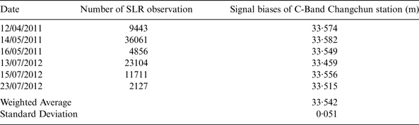
Table 3 gives the signal biases of the Changchun C-Band station using the co-location comparison method. From this table, the weighted average signal biases of the Changchun C-Band station is 33·542 m with a standard deviation of 0·051 m.

Table 3.

The signal biases of Changchun C-Band station using the co-location comparison calibration method.

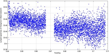
Figure 3 gives the signal biases of the Changchun C-Band station on 13 July 2012. Due to the motion of the GEO satellite, there are differences between the bias estimates at each epoch. The GEO satellite is not motionless, with the ground track of the satellite forming a figure of eight.

Figure 3.

The signal biases of Changchun C-Band station on 13 July 2012.

3.2. The signal biases calibration for the Linton and Kashi C-Band stations using the combined POD method

After the signal biases of the Changchun C-Band station have been calibrated, the signal biases of the other two C-Band stations can be obtained by the combined POD method using the SLR and CAPS CBTR observations. It is worth mentioning that the Changchun C-Band station's signal biases have been fixed in the combined POD process using the kinematic batch processing method (Tapley et al., Reference Tapley, Schutz and Born2004).

The adopted astronomical constants, reference system, dynamical and measurement models are referred to IERS Conventions 2003 (McCarthy and Petit, Reference McCarthy and Petit2004). The reference systems involved are (1) the inertial J2000·0 system, (2) ITRF2000 for the coordinates of the stations and their velocities of motion (Altamimi et al., Reference Altamimi, Sillard and Boucher2002), and (3) the planetary ephemeris DE403/LE403 (Li et al., Reference Li, Qiao and Feng2006). The parameters involved to set up the rotation matrix between different coordinate systems are (1) the precession model IAU1976 (Lieske et al., Reference Lieske, Lederle, Fricke and Morando1977), (2) the 1980 nutation model (Wahr, Reference Wahr1981; Seidelmann, Reference Seidelmann1982), and (3) the EOP 08 c04 containing the polar motion parameters, dUT1 and the nutation correction (Huang et al., Reference Huang, Hu, Zhang, Zhang, Guo, Wang and Shi2011; Song et al., Reference Song, Mao and Jia2012; Cao et al., Reference Cao, Yang, Su, Li, Feng, Sun, Yang and Kong2014a; Cao et al., Reference Cao, Yang, Su, Li, Chen, Li, Sun, Kong, Wei and Feng2014b).

The dynamic acceleration consists of the following: (1) two-body gravitational attractions of the Earth, (2) N-body gravitational attractions of the Sun and Moon, (3) relativistic perturbation, (4) gravitational attractions of the non-spherical Earth (Earth gravity model JGM3, truncated to the 10th degree and order) (Tapley et al., Reference Tapley, Watkins, Ries, Davis, Eanes, Poole, Rim, Schutz, Shum, Nerem, Lerch, Marshall, Klosko, Pavlis and Williamson1996; Xu, Reference Xu.2007; Xu and Xu, Reference Xu. and Xu2013), (5) gravitational attractions of solid-Earth tides, oceanic tides and atmospheric tides (Wahr, Reference Wahr1981; Li, Reference Li1995; McCarthy and Petit, Reference McCarthy and Petit2004; Xu, Reference Xu.2007; Xu and Xu, Reference Xu. and Xu2013), (6) perturbation of Earth's rotational deformation (Buffett et al., Reference Buffett, Mathews, Herring and Shapiro1993), (7) radiation pressure of the Sun (Parkinson et al., Reference Parkinson, Jones and Shapiro1960; McCarthy and Petit, Reference McCarthy and Petit2004; Tapley et al., Reference Tapley, Schutz and Born2004; Xu, Reference Xu.2007; Xu and Xu, Reference Xu. and Xu2013), (8) Earth albedo radiation pressure (Sehnal, Reference Sehnal1980; Borderies and Longaretti, Reference Borderies and Longaretti1990) and (9) empirical radial-transverse-normal accelerations (Eanes and Bettaadpur, Reference Eanes and Bettaadpur1996; Huang et al., Reference Huang, Hu, Zhang, Zhang, Guo, Wang and Shi2011; Cao, Reference Cao2014c).

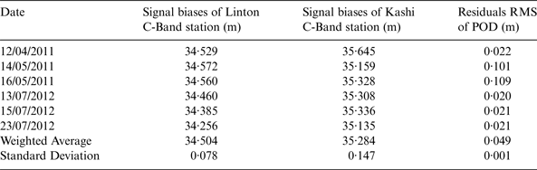
In the process, one day arcs have been adopted, with the initial satellite orbits, solar radiation pressure parameters and the signal biases of the Linton and Kashi C-Band stations to be estimated. Table 4 shows the signal biases of the Linton and Kashi C-Band stations obtained from the combined POD method. From this table, it can be seen that the weighted average sum of the signal biases for the Linton C-Band station is 34·504 m with a standard deviation of 0·078 m. The weighted average sum of the signal biases for the Kashi C-Band station is 35·284 m with standard deviation of 0·147 m.

Table 4.

The signal biases of Linton and Kashi C-Band stations using combined POD method.

4. THE EFFECT ON POD PRECISION BEFORE AND AFTER SIGNAL BIASES CALIBRATION

In order to evaluate the precision of signal biases calibration, two POD experiments using the GEO satellite (COSPAR ID 2010-001A) have been conducted. The adopted astronomical constants, reference system, dynamical and measurement models are the same as those in the combined POD (See Section 3.2).

Firstly, a POD for the GEO satellite is performed before the signal biases calibration. One day arcs have been adopted, with the initial satellite orbits, solar radiation pressure parameters and transponder delays to be estimated. The station deviations are obtained by successive approximation (Cao et al., Reference Cao, Yang, Li, Sun, Kong, Chen and Feng2014d). The signal biases can then be calculated by adding the transponder delays and station deviations for each station and day.

Then, POD for the GEO satellite has subsequently been conducted by fixing the signal biases in Tables 3 and 4. Also one day arcs have been adopted, with the initial satellite orbits, solar radiation pressure parameters to be estimated.

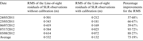
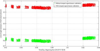
Both orbit sets have been evaluated using the SLR observations to get the line-of-sight residuals of the SLR observations. Note that the SLR observations are not employed in the calibration process. Table 5 lists the RMS of the line-of-sight residuals of the SLR observations for the two orbit sets and the percentage improvements for the RMS.

Table 5.

Line-of-sight residuals of SLR observation without and with signal biases calibration.

Figure 4 shows the line-of-sight residuals of the SLR observations without and with signal biases calibration on July 17th, 2012. From Figure 4 and Table 5, it can be seen that the line-of-sight residuals of the SLR observations are 0·532 m without the signal biases calibration. After calibration, the residuals decrease to 0·132 m. The RMS of the line-of-sight residuals have been improved by 75·19% after the calibration, clearly demonstrating that the precision of the POD has increased after signal biases have been calibrated in CAPS.

Figure 4.

Line-of-sight residuals of SLR observation without/with signal biases calibration on 17 July 2012.

Due to the motion of the GEO satellite, there are differences between the line-of-sight residuals at each epoch. The GEO satellite is not motionless, with the ground track of the satellite forming a figure of eight. The orbit period of the GEO satellite is about 24 hours. However, the SLR observation arc cannot cover the whole period, which leads to the offsets in the line-of-sight residuals in Figure 4.